Introduction

Prior to the last decade, it had generally been assumed that glaciers moved over rigid substrata and that the rheology οf ice and the processes of sliding of ice over this rigid bed determined the dynamic response of the glacier, to changes in surface mass balance (Fig. la and b).

Fig. 1.

Schematic diagrams showing the horizontal velocity distribution in sections through a glacier resting on: (a) a frozen bed (rock or unlithified sediment): (b) a rigid bed but with sliding along an unfrozen glacier/bed contact: (c)a deforming bat. There are three possible velocity components: internal flow (U_f): basal sliding (U_s): deformation of subglacial sediments (U_D). If the longitudinal ice flux is approximately constant in all cases. it will be discharged through a progressively thinner, lower-sloped glacier in going from case (a) to case (c).

Similarly, it had been implicitly assumed that the processes of erosion and deposition which occur when glaciers flow over rock beds were universally applicable. In these processes, subglacially crushed detritus is incorporated in the ice by freezing. transported englacially and released basally from the glacier by lodgement or supraglacially by melting-out. No-one had explicitly addressed the question of erosion and deposition on beds of unlithified sediment.

However, many modern glaciers rest, at least in part, on unlithified beds, and large areas of the Pleistocene ice sheets in the mid-latitudes of Europe and North America were underlain by thick, unlithified sediment sequences. Under-standing erosion and deposition on such a bed is thus important: not only for geological reasons but because the strong coupling which it is suggested can occur between the glacier and such a bed can have a major influence on a glacier’s dynamics and its role in climate change.

Reference Boulton and JonesBoulton and Jones (1979) suggested that the rheology of deforming subglacial sediments could be a major determinant of the dynamic behaviour of ice sheets (Fig. lc). Reference Alley, Blankenship, Bentley and RooneyAlley and others (1987) demonstrated the reality of this process beneath the West Antarctic ice sheet and that the dynamics of at least one of its major ice streams was largely controlled by the deformation of water-soaked sediment. Reference Engelhardt, Humphrey, Kamb and FahnestockEngelhardt and others (1990) confirmed, by drilling, the presence of such sediment. Reference Boulton, Menzies, Rose and RotterdamBoulton (1987) explored the consequences of subglacial deformation for processes for process of erosion and deposition, and suggested that, in the sediment-covered lowlands which underlay much of the outer zones of mid-latitude ice sheets, sediment deformation played the dominant role in glacial erosion and deposition and in the production of tills and drumlins, and that most of the constituents of such tills had not been transported by conventional englacial mechanisms.

This paper develops a theory of large-scale erosion and deposition produced by an ice sheet resting on an unlithified sediment bed. For the sake of simplicity, it is assumed that such a bed occurs beneath the whole of the ice sheet. For the ice sheets which covered large parts of North America and northwest Europe during the last glacial period, much of the outer zones were underlain by soft sediment and the inner zones predominantly by bedrock. Although a complete description of subglacial erosion and deposition requires integration of “hard-bed” and “soft-bed” theories, it will be argued in a later paper that the approach taken below can be applied to both and therefore that the conclusions of this paper can be applied qualitatively to a “hard bed”.

The effects of fluvial reworking of till are ignored in the theory. Not because they are not important but because they are superimposed upon the patterns predicted here, and it is the reality of those primary patterns which will test the theory. A fluvial reworking theory, though desirable, can be regarded as a separate issue.

Erosion, Transport and Deposition on an Unlithified, Deforming Bed

Consider a glacier whose sole is at the melting point and underlain by unlithified sediments into which subglacial meltwater is discharged. Reference Boulton and JonesBoulton and Jones (1979) showed that, beneath a large glacier, any significant thickness of fine-grained (clay- or silt-rich) sediment would be enough to impede interstitial drainage to the extent of producing zero effective pressure in the sediment, resulting in little or no frictional resistance beneath the glacier and producing “unstable” deformation which could lead to a surge. Reference Boulton and HindmarshBoulton and Hindmarsh (1987) suggested, however, that unstable deformation at zero effective pressure would lead to “piping” so as to produce sediment-floored tunnels which would drain excess water and re-establish stable deformation and restabilize the sediment/glacier system. An equilibrium would be maintained in which major perturbations which tended to increase interstitial water pressures would be counteracted by the production of further tunnels or the enlargement of existing ones, whilst reduction in water pressure would be counteracted by tunnel closure. It was suggested that the subglacial system thus adjusts itself to climatically determined ice discharge and, notwithstanding the potentially complex behaviour of subglacial till (Reference ClarkeClarke, 1987), the average frictional resistance which a given bed offers to a given glacier need not be highly variable. It is argued thus that there are internal mechanisms which buffer external perturbations and maintain stable operation of the system.

From the observations of Reference Boulton and JonesBoulton and Jones (1979) and Reference Boulton and HindmarshBoulton and Hindmarsh (1987) at the Breiðamerkur-jökull experimental sites, and their theoretical explanations, it is suggested that subglacial shear deformation occurs when subglacial drainage is so poor that high pore-water pressures, and therefore low effective pressures, develop in the sediments immediately beneath the glacier sole above a level z _A. where effective pressures are no longer large enough to prevent deformation (Figs 1c and 2). This defines a tectonic A horizon within which shear deformation tends to cause dilation of the grain skeleton, producing a much lower density than in the underlying, undeformed and consolidated Β horizon.

Fig. 2.

The pattern of effective pressure, stress and strain in a deforming subglacial sediment. (a) shows the distribution of Subglacial effective pressure which determines the sediment shear strength. Effective pressure at the glacier sole will be finite or zero. (b) shows an increasing sediment shear strength with depth which is a linear function of effective pressure. and which eventually exceeds the constant value of shear stress at depth t_A, below which no further deformation will occur. (c) shows the distribution of strain rate in the deforming A horizon, overlying a stable B horizon. Strain rate depends on shear stress and sediment strength.

A Coulomb failure criterion is used to define the shear strength (σ) of the sediment:

(1)

where c is the cohesion, Φ is the angle of internal friction of the sedments and p ¹ is effective pressure. Beneath the glacier sole, p ¹ will increase with depth in the following way (Fig. 2a):

(2)

where n is the void ratio of the sediment, ρ _s is the density of sediment grains, ρ _w is the density of water. m is the basal melting rate. k is the sediment permeability and g is the acceleration due to gravity. (1 — n)(ρ_s — ρ_w)g is a term which describes the increase of buoyant weight with depth, and (mρ_w/k)g. a term due to the potential gradient generated by the flux of meltwater (m) through the sediment. If the sediment has a relatively high permeability, greater than about 10⁷–10 m s⁻¹ (Reference Boulton and DobbieBoulton and Dobbie, 1993), the potential gradient δp′/δz within it will be a typical gravitational gradient of about 10 k Pa m⁻¹. Under this latter circumstance, the second term on the righthand side of Equation (2) will be zero, as it will be if there is no vertical water flux.

The effective pressure P¹ at any depth (z) will be:

(3)

where is the effective pressure at the glacier sole. The shear Stress at the base of the glacier (T_b) is assumed to be constant with depth in the sediment, whilst P¹ increases with depth (Fig. 2a and b). Deformation will cease at a depth (Z_A) where shear stress equals shear strength (T_b = σ):

(4)

so that

(5)

Reference Boulton and HindmarshBoulton and Hindmarsh (1987) suggested two flow laws for a deforming sediment, one of which assumed non-linearly viscous behaviour so that:

(6)

where is the shear strain rate and A, n and m are constants. The A/B interface is assumed to form a rigid surface above which sediment in the A horizon deforms as a viscous fluid. The velocity (U) at any point in the A horizon, due to incremental strain within it, is found by integrating from the base of the deforming A horizon:

(7)

Substituting Equations (3) and (6) into Equation (7) gives:

(8)

δp′/δz can be regarded as constant. The equation is solved numerically.

The horizontal flux of sediment within the deforming A horizon (Q _A) will be:

(9)

which is also solved numerically.

If, in a steady state, the flux of sediment increases in the down-glacier direction (δQ _A/δx positive), more material must be added to the deforming A horizon in order to maintain continuity (Fig. 3a). This can only be achieved by progressively lowering the interface between the deforming horizon and the underlying. hitherto stable horizon, which is thereby eroded by being drawn into the flow. The hitherto stable bed is eroded because of the increasing flux in the A horizon and the A/B plane is lowered. Conversely, if the sediment flux diminishes down-glacier (δQ _A/δx negative). mass must be lost from the deforming horizon (Fig. 3b), which will occur by hitherto mobile material accumulating at the base of the deforming horizon and resulting in a rise of the A/Β plane.

The rate of erosion will be:

(10)

Erosion will occur when (E) is positive and deposition when negative. In the erosional case, sediment passes from the stable to the deforming horizon and in the depositional case from the deforming to the stable horizon. For the purpose of this paper, a thick stratum of unlithified material is assumed. If lithified bedrock is exposed during erosion, the mechanism of erosion will change and the rate of erosion will he reduced.

Fig. 3.

The conditions for erosion and deposition on a deforming bed. In (a), longitudinally or temporally increasing ice flux is associated with higher shear stress and increasing sediment discharge, causing material from the stable B horizon to be added to the mobile A horizon, lowering of the A/B interface and erosion. (b) shows the converse case of deposition resulting from longitudinal compression.

Patterns of Soft-Bed Erosion and Deposition beneath a Steady-State Ice Sheet

It is clear that there is strong coupling between the dynamics of an ice sheet and sediment deformation beneath it. A steady-state ice-sheet profile must be compatible with the deforming-bed rheology and the ice-sheet surface mass balance. Flow in the bed will be driven by the basal shear stress, given by the ice-sheet profile, and the bed rheology will depend upon the subglacial effective pressure distribution, which is a function of the melting rate and drainage. We therefore seek a relationship between mass balance, shear stress and effective pressure. Reference Boulton and JonesBoulton and Jones (1979) analyzed the coupling between ice-sheet mass balance and shear stress for a bed of given rheology, assuming a constant effective pressure in the bed. Unfortunately, we still do not have an adequate physical understanding of subglacial drainage processes in order to analyze the hydraulic component of effective pressure and therefore to analyze the full coupled system.

Reference RöthlisbergerRöthlisberger (1972), Reference WeertmanWeertman (1972) and Reference NyeNye (1973) analyzed the flow of water in tunnels over a rigid bed. Reference AlleyAlley (1992) showed that tunnels on the deforming bed of a glacier could not be fed from water flowing at the glacier/bed interface. Reference Fowler and WalderFowler and Walder (1993) suggested that drainage in such a situation might occur through “canals” in the till, and Reference Clark and WalderClark and Walder (1994) suggested that the abrupt termination of eskers at the edge of the shield areas in Europe and North America might reflect a change from tunnels to canals. Reference Boulton, Slot, Blessing, Glasbergen and van GijsselBoulton and others (1993, paper in preparation) have demonstrated that ground-water flow can play a major role in ice-sheet hydraulics. However, more work is required before these processes can be integrated in such a way as to provide a drainage theory which relates effective pressure to ice-sheet dynamics and so permits a properly coupled sheet/sediment dynamics problem to be solved.

It is therefore assumed that shear stress distribution is known, and from this is calculated the effective pressure and distribution of sediment deformation which would be compatible with it for a given ice-sheet-surface mass-balance distribution. A constant basal effective pressure could equally be assumed and the shear stress and sediment deformation calculated which would be compatible with this for a given mass balance. The resulting general patterns of erosion and deposition are similar.

It is assumed that there is no slip between a sediment bed of constant lithology and the ice-sheet sole (it would be a simple matter to include slip), and that the forward movement of the ice sheet is entirely accounted for by deformation. A similar approach was successfully used by Reference NyeNye (1959) to compute the theoretical profile of an ice sheet. He argued that most of the flow of an ice sheet occurred at or near its bed and thus that its longitudinal profile could be modelled by assuming basal sliding but no internal flow. Using a sliding law of the form U _b = Bτ _b ^n–1 where B and n are flow-law parameters, he showed that the profile should be

(11)

where H is the ice thickness at the divide, L is the distance from the divide to the terminus, h and x are local ice thickness and distance from the divide, respectively, and b is a flow-law parameter.

As a flow law for deforming sediments (Equation (6)) is similar to that for ice, and as effective pressure has been suggested as having a similar role in governing friction on a hard bed (Reference MorlandMorland, 1984) as on a soft bed, we might expect a profile similar to that described by Equation (11) to apply to a deforming bed, although with different parameters. This should apply unless there is a major change in fundamental properties of the bed. such as the change from granitic rocks with little soft-sediment cover to sedimentary rocks with an ample soft-sediment cover, where Reference Boulton and JonesBoulton and Jones (1979) suggested that a “Mexican hat“ profile could develop. In such a case, as in the case of a rigid bed. we might expect the drainage system to adapt itself, much as it is presumed to do on a hard bed, to control effective pressures so that flow in the till layer discharges the appropriate ice-mass flux. A generalized mechanism for effective pressure control was suggested by Reference Boulton and HindmarshBoulton and Hindmarsh (1987) and has been amplilied by Boulton and others (paper in preparation). That there is a mechanism which controls effective pressure in the case of a soft bed is strongly suggested by the measurements of Reference FountainFountain (1994) on the South Cascade Glacier, which does not appear to have a history of surging, where a subglacial sediment layer is assumed and where effective pressures are uniformly between 100 and l50 kPa, except in the vicinity of a subglacial channel. This would produce conditions very close to failure in most coarse-grained tills along most of the length of the glacier.

It has therefore been assumed that an ice sheet on a deformable bed with uniform bydrogeological properties will have a parabolic profile of the general form given by Equation (11).

It is assumed that movement occurs as a result of displacement at the ice/bed interface due to shear in underlying sediments (sliding is assumed not to occur at the ice/bed interface because of the roughness of an ice/sediment interface). The ice discharge due to deformation in underlying sediments will be:

(12)

where U _b is the velocity at the ice/bed interface (given by Equation (8) integrated to z = (0). The ice discharge is a function of mass balance (α), which is positive in the accumulation area and negative in the ablation area:

(13)

where ρ _i is ice density and x is the distance from the ice divide. Combining Equations (8), (12) and (13) gives:

(14)

Values of which are compatible with values of U _b and the values of T _b given by Equation (11) are derived by integration of Equation (8) to the glacier sole:

(15)

Results are shown in Figure 4 for an ice sheet of 500 km span, a divide elevation of 2.8 km, a mean accumulation rale of 0.5 m a⁻¹ and for a sandy Icelandic till, a silty till from The Netherlands (Table 1) and a clay till.

Table 1.

Values of non-linearly viscous flow-law parameters for a sandy till from bredamerkujojull, a sillly saalian till from the Netherlands and a clay quoted by Reference KambKamb (1991). No Aparameter can be inferred for the clay-rich till from Reference KambKamb’s (1991) paper

Fig. 4.

Idealized conditions at the bed of a steady-state ice sheet underlain by a deformable bed for a given ice-flux distribution. Conditions are calculated for clay, silt and sandy the beds. (a) Thickness of the deforming horizon (b) The discharge within the deforming horizon. (c) Erosion and deposition rates. (d) Effective pressure at the glacier sole.

The analysis implicitly assumes that a mechanism exists to adjust the effective pressure at the glacier sole, and thereby deforming layer thickness, so that the basal velocity is able to balance the ice flux. As can be seen in Figure 4d, the effective pressure must remain relatively constant along the flowline in order tο maintain stable deformation.

Figure 4 also shows calculated values of deforming horizon thickness (Fig. 4a), discharge in the deforming horizon (Fig. 4b) and rates of erosion and deposition (Fig. 4c).

The thickness of the deforming horizon increases from zero beneath the divide region to a maximum in the vicinity of the equilibrium line and decreases to zero at the terminus. Both the mean velocity and discharge show a similar pattern, although they are slightly offset in relation to each other. The rate of erosion is zero or very low in a broad region near to the divide and rises to a maximum just up-glacier of the equilibrium line, where the rate of increase of discharge in the deforming horizon is greatest. It then decreases to zero beneath the equilibrium line, beyond which We pass to a zone of deposition.

The Role of Sediment Grain-Size in Erosion, Deposition and Glacier Dynamics

The till produced by Pleistocene ice sheets in mid-latitude lowlands are predominantly silt-rich, although some are clay-rich and some sand-rich. Table 1 shows values ol flow-law parameters for an Icelandic till (Reference Boulton and HindmarshBoulton and Hindmarsh, 1987), a Saalian-age till from the Netherlands (Reference DobbieDobbie, 1992) and for a clay-rich till (Reference KambKamb. l991). They are formulated for the non-linearly viscous model . Figure 5 illustrates the different responses of granulometrically different tills. The effective pressure at the glacier sole and the velocity profile in each till has been calculated (from Equation (8)) which would generate the same basal ice velocity (Equation (15)) under the same shear stress. The clay till is clearly softest and the sandy till hardest. As a consequence, the deforming-layer thickness needs to be greatest in the sandy till where the strain rate is relatively small and least in the clay till where the strain rate for the same Stress is very large (Fig. 5). The effective pressure at the top of the sandy till needs to be very small to ensure that the till is soft enough to deform to relatively great depth and also relatively small in the clay till to offset the relatively large cohesion of clay (Fig. 5).

Fig. 5.

The influence of granulometry on till behaviour. It is assumed that the ice flux in the glacier is discharged only as a result of deformation of the bed. We contrast a glacier driven by a relatively high shear stress (a) With one driven by a relatively low shear stress (b). The effective pressure at the ice/bed interface and the thickness of the deforming layer are calculated for three till types (sand-rich, silt-rich, clay-rich) so as to yield basal velocities of 150 m a⁻¹ and 70 m a ⁻¹ with shear stresses of 75 kPa and 25 kPa, respectively. Deforming layer thickness (t_A), effective pressure and discharge in the deforming layer (Q_A) for the sand, silt and clay materials are shown in the boxes. Ίο sustain a given velocity, deformation depth and discharge rates (and therefore erosion rates) are greatest for a sand under the smallest values of . A very small change in effective pressure produces a very large change in strain rate for a day. In the limit, deformation on a clay surface is analogous to sliding, with a very small discharge and erosion rate.

The sediment discharge in the deforming horizon is greatest for the sandy till and least for the clay till, which also reflects their erodibility (Fig. 5). This is, however, a potentially misleading consequence of the assumption that effective pressure is given and ignores the role of sediment permeability in controlling drainage (Reference Boulton and DobbieBoulton and Dobbie, 1993). The sandy till will tend to drain relatively well, leading to high effective pressures, which will inhibit deformation. Shear stresses will therefore build up and the internal flow and sliding components of glacier movement (Fig. 1c) will become larger. Conversely, silty and clayey tills will tend to impede drainage and to scal off any subglacial aquifers so that low effective pressures can be readily maintained. One might therefore expect silty sediments to be the most susceptible to erosion and silty tills to dominate where there is an appropriate sediment supply. Most tills derived from sources where there is a wide range of grain-size available are indeed silt-dominated (Reference EylesEyles, 1983).

The three different sediment types have very different strain-rate sensitivities to changes in effective pressure. For instance, for a constant shear stress of 40 kPa, unit decrease in effective pressure produces changes in strain rate as shown in Table 2.

Table 2.

Change in effective pessure required to produce 10-, 100- and 10 000-fold increases in strain rate in sand, silt and clay tills, respectively, for a constant shear stress of 40 KPa. Righthand column shows strain-rate sensitivity to unit decrease in effective pressure

In response to a perturbation in shear stress or effective pressure, we would expect the sandy till to be most readily stabilizeable through water-pressure adjusi-ments in the subglacial channel system and clay tills to be least stabilizeable. The very low permeability of clays may give them a very slow response time to external water-pressure changes (Reference Boulton and HindmarshBoulton and Hindmarsh, 1987) and thus be a partial buffer to instability. Although firm conclusions should await a time-dependent analysis, it seems probable that subglacial channel control might permit stable deformation of sand- and silt-rich tills but not Of clay-rich tills. Subglacial clays are therefore liable to be a considerable cause of instability, which is reflected, I suggest, by their common occurrence along major planes of tectonic transport in subglacial sediments.

Time-Dependent Patterns of Erosion and Deposition Produced during Glacial Cycles

Much of the lowland area of Europe and North America which has suffered ice-sheet glaciation during the last million years is covered by soft, deformable sediment and should carry evidence of patterns of erosion and deposition Which the theory should be able to explain. However, residual patterns of erosion and deposition will reflect integrated behaviour over complete glacial cycles rather than merely an ice sheet’s geological activity during the glacial maximum, as has been assumed in some erosional theories (e.g. Reference WhiteWhite, 1972; Reference SugdenSugden, 1977). It is important therefore that the theory is extended to the time-dependent case. To achieve this, the mass-balance distribution is changed and the function h(x, t) estimated using the continuity equation for ice thickness:

(16)

This yields a time-dependent distribution of velocity and shear stress, although the flow field is equivalent to a series of steady states. Values of effective pressure at the ice/bed interface which are compatible With values of basal shear stress and velocity are determined from Equation (15). The erosion/deposition rate is then integrated with respect to time (t).

The time-dependent evolution of an isothermal ice sheet on a horizontal bed driven by a prescribed positive mass budget has been simulated. The equilibrium line was fixed at 60 km from the terminus. The net annual accumulation rate was constant at 1.0 m a⁻¹. The net annual ablation rate increased linearly from zero at the equilibrium line to a maximum at the terminus. Ice-sheet growth was produced by imposing an average budgetary excess of 45% on the south side of the ice sheet and 30% on the northern side. These were switched to deficits of similar proportions after 12000 years in order to produce retreat. The maximum net ablation rate was adjusted to achieve the required budgetary excesses/deficits. From this, the mass-balance velocity through the glacial cycle was calculated and the magnitudes of erosion and deposition determined as described above.

Results are shown in Figure 6 for an ice sheet lying on a horizontal sediment bed of sandy till which is assumed to be at the melting point throughout. Figure 6a (1-5) shows the progressive evolution of a sediment surface at a series of times during the growth phase of the ice sheet. During expansion, the proximal zone of erosion expands and the distal zone of deposition is progressively displaced outwards as a wave-like form. In the erosional zone, the A/B décollement descends. In the depositional zone, the A/B plane migrates upwards as deposition proceeds but is then succeeded by downward migration of the A/Β plane as the erosional zone expands. During retreat (Fig. 6b, 5–10), further erosion occurs in the proximal zone but, as the distal zone of deposition withdraws over the eroded surface, a retreat phase till is deposited.

Fig. 6.

Progressive evolution of the sediment bed of an ice sheet during its advance and retreat phases. (a) 1 5 show stages in the evolution of the bed and contemporary ice margins during the advance phase. The horizontal line shows the original position of the pre-glacial surface, and the shaded surface the position of the bed at the end the advance phase. Deformation produces erosion and lowering of the bed in the up-glacier zone, and deposition and elevation of the bed in the terminal zone. A wave of deposition sweeps outwards beneath the advancing glacier, followed by progressive extension of the erosional zone. Any point lying initially beyond the glacier is first covered by an increasing till thickness in the depositional zone. Subsequent erosion first thins the till and then erodes beneath the original surface. (b)The further evolution of the bed during ice-sheet retreal. The initial form of the uneroded substralum bed is shown by 5 and the final form by 10. Thick lines show where the bed is made of deposited till at each stage of retreat. In this model, the retreat phase is taken to be longer than the advance phase, resulting in greater net erosion during retreat

The pattern of erosion and deposition during the whole cycle is illustrated in Figure 7a by the time space envelope for a mid-latitude ice sheet expanding from an initial nucleation point, both to the north, where it will be limited by moisture starvation and the ocean margin, and to the south, where it will be limited by high surface-melting rates. The ice sheet then contracts to the area in which it first began to develop. The mass-balance distribution was adjusted to produce a temporally symmetrical cycle. During an ice sheet’s decay phase, the zones of erosion and deposition contract and, as the depositional zone retreats over a previously eroded surface, a capping of till accumulates.

Fig. 7.

(a) Time-space envelope of an ice sheet during a simple glacial cycle and the history of erosion and deposition at specific sites (A-I). At these sites, vertical lines show the original surface and a further line shows its erosional/depositional evolution. At B-H, till is first deposited as the glacier over-rides the sites. In the succeeding erosional zone, the advance-phase till is removed until erosion bites down beneath the original substratum, and a final retreat-phase till is then deposited on the eroded surface. At A and I, deposition during the retreat phase recommences before all the advance-phase till has been eroded, resulting in two tills with an intervening erosion surface (possibly marked by a boulder pavement). The extreme northern and southern marginal zones at the minimum lie entirely in the depositional zone, and so till deposition is continuous, though the rate varies. If the ice divide were stationary, no erosion would occur beneath it. Erosion here only occurs because of the divide shift. (b) The resultant pattern of erosion and deposition at the end of the glacial cycle. There are four principal zones: an ice-divide zone of little erosion and thin retreat-phase tills: an intermediate zone of strong erosion and thicker retreal-phase tills; a zone of thickest till, resting on an uneroded substratum, comprising a lower, advance-phase till, separated by an erosion surface from the retreat-phase till; an outer zone of thinner till in which the advance-phase till grades upwards into the retreat-phase till.

The histories of a series of sites (A-I) are followed through the glacial cycle as zones of erosion and deposition expand and contract. In the inner zone (G-H), the initial phase of depositon is short. In the succeeding erosional phase, the pre-existing till is soon removed and erosion cuts down into hitherto undeformed sediments. As the glacier expands further, the erosion rate decreases, increases again after the glacial maximum and finally diminishes before it gives way to a phase of deposition just before deglaciation of the site. At sites A and I, the erosional phase is not long enough for the advance-phase till to be entirely removed before deposition recommences during glacier retreat, producing two till units with an intervening erosion surface. Αt these sites there is no erosion of preglacial beds. Very close to the overall terminus, there is no cessation of deposition but the deposition rate does vary, being least during the phase of most extensive glaciation.

The net result of this cycle of erosional and depositional activity is shown in Figure 7b. Four major zones are identified:

• Zone 1. The ice-divide zone, with slight erosion and a thin till deposited during the retreat phase.

• Zone 2. A zone of strong erosion with a till derived from the retreat phase only.

• Zone 3. A zone of no erosion of preglacial beds overlain by a thick till sequence containing both advance- and retreat-phase tills but with an intervening erosional interface.

• Zone 4. A zone of no erosion of preglacial beds overlain by a thick till sequence continuously deposited throughout the local glacial cycle.

Because of the greater expansion to the south compared with the north, the ice divide also migrates to the south during expansion and returns north to its original position during decay. It is import ant to note that, if the ice divide in an ice sheet were to remain stationary through the whole glacial cycle, there would be neither significant erosion nor deposition beneath it, as the horizontal ice velocity tends to zero beneath the divide. Only movement of the divide through the cycle, as a consequence of a changing centre of mass which reflects ice-sheet/atmosphere interaction (Reference Boulton and ClarkBoulton and Clark, 1990) ensures that erosion and till deposition will take place in the divide/zone.

The predictions of the theory are contrary to the views of Reference WhiteWhite (1972) who argued that deep erosion is concentrated beneath the central parts of ice sheets.

Figure. 8 shows a model run in which an average 30% mass-balance excess during ice-sheet build-up on its southern flank is sustained for 20000years and an average deficit of 36% during retreat. This produces an asymmetric pattern of growth and decay similar to the presumed normal pattern during late Quaternary, glacial periods. Reference Hindmarsh, Boulton and HutterHindmarsh and others (1989) have suggested that mid-latitude ice sheets in Europe and North America had a broad ice-divide zone and a narrow terminal zone where basal temperatures were below the melting point, and a broad intervening zone in which melting occurred. Reference Boulton and PayneBoulton and Payne (1992) suggested that as much as 800 km on the southern flank of the European ice sheet at the glacial maximum underwent basal melting, beyond a 200 km zone beneath the divide in which temperatures were below the melting point. Moreover, they showed that the distribution of basal melting/freezing was relatively insensitive to precise values of surface temper-ature and mass balance, provided that the atmospheric lapse rate lay Within the range of modern values. The basal melting/freezing distribution for the glacial cycle shown in Figure. 8a is based on typical patterns produced by the Boulton and Payne model. It shows temperate basal Conditions during the advance phase in the outer part of the ice sheet, extending to over half the ice-sheet span. During the decay phase, however, retreat of the ice front is much more rapid than retreat of the temperate/cold thermal boundary (Reference Boulton and PayneBoulton and Payne, 1992), so that in the late stages the whole of the base of the ice sheet lies below the melting point.

Fig. 8.

(a) A diagram similar to Figure. 7a but showing an asymmetric cycle for a semi-span, in which the period of build-up is longer than the period of decay, and in which there is a frozen-bed zone beneath the divide area. Some erosion occurs in the divide zone during build-up but no till is deposited there during retreat as the bed remains frozen during deglaciation. (b) The resultant pattern of erosion and deposition. (c) The potential relief of drumlins assuming an inexhaustible sediment supply and uniform bed materials. It shows phases of deposition then erosion during the advance hemi-cycle and erosion then deposition during the retreat hemi-cycle

The importance of thermal regime lies in the assumption that there will be no sliding motion between a glacier sole and bedrock where the interface is below the melting point (Reference GoldthwaitGoldthwait, 1960), because of the large shear strength of such a contract (Reference JellinekJellinek, 1959). I assume that this applies not only to bedrock but also to frozen sediment. It is also assumed that no erosion will occur at such a contact, apart from large-scale bedrock detachment (Reference MackayMackay. 1959: Reference Boulton and CoatesBoulton. 1974). Several major geomorphological contrasts have been explained as a consequence of suppression of erosion by frozen-bed conditions (Reference SugdenSugden, 1977: Reference BoultonBoulton. 1979; Reference Andrews, Clark, Stravers and AndrewsAndrews and others, 1985: Reference KlemanKleman. 1990; Reference LagerbäckLagerbäck, 1990).

Inclusion of the basal thermal regime generates an additional effect (Fig. 8b). In the internal zone, erosion occurs and till accumulates during the early phase of growth when the bed is unfrozen but extension of the frozen zone inhibits further erosion and leads to preservation of early tills and erosional features. These are not subsequently eroded, as the internal zone remains a zone of basal freezing until deglaciation.

Sediments of the A Horizon as Tills

Figure. 5 suggests that sediments in the deforming A horizon can readily attain velocities in excess of 100 m a ⁻¹ and strain rates in excess of 50–100 a⁻¹ under relatively low shear stresses. Velocities averaged over periods of days to weeks in the A horizon beneath Breiðamerkur-jökull. Iceland, vary from 10 to 64 m a⁻¹.

Observations at Breiöamerkurjökull (Reference Boulton, Menzies, Rose and RotterdamBoulton, 1987) show that local inhomogeneities and high shear strain rates within the A horizon generate folding episodes. If these episodes are frequent, they have the capacity to mix thoroughly and homogenize the sediment, leaving no markers by which folding may be recognized. I suggest that sediment deposited from this horizon should be regarded as a primary sediment produced by ice rather than as a pre-existing sediment which has merely been tectonized. Reference Boulton, Menzies, Rose and RotterdamBoulton (1987) suggested that the term deformation till should be applied to it.

Reference Ehlers, Gibbard and RoseEhlers and others (1991) commented that the relativerarity of deformational structures at the base of tills or in sub-till sediments in the area occupied by the European ice sheet implies that deformation tills are unlikely to be the dominant till type in Europe. Such conclusions reflect misunderstanding of the sedimentary consequences of the deformation process. Consider the base of the deforming horizon in the erosional zone. As the A/Β plane descends, hitherto undeformed sediment is drawn into the A horizon flow. This may be on a grain-by-grain basis or as thin cohering layers. The Α/B plane may, however, be rough or the sediment drawn into the flow may be stiffer than the deforming sediment around it, in both of which cases stress concentrations will develop and folding will occur and, it sufficiently frequent, will eventually homogenize the sediment. Eroded sediment will be transported in the A horizon and, at some distance from its source, will eventually be deposited as till. During transport we expect shear strain rates (Fig. 5) of the order of 10–100 a⁻¹. Such rates would reduce a 1 m high vertical structure produced by folding during incorporation to a dip of 0.5–0.05° alter only 2 years of transport and during the same period would attenuate it horizontally by 10–100 m. Only if the sediment is “frozen” by deposition shortly after folding of an unhomogenized sediment will folds with steep limbs survive. Deposition after further folding and attenuation will tend to produce the commonly found laminated tills, and deposition after longer transport will produce homogenized tills (Reference Boulton, Menzies, Rose and RotterdamBoulton, 1987).

It is suggested that three basic deformation till facies can be identified which reflect progressively greater incremental strain. They are

In general, the more obvious the tectonic structures, the less the incremental deformation. Moreover, a consequence of long-term erosion of a surface by deformational lowering of the A/Β plane will be progressive smoothing of the surface. Protruberances on an originally rough surface will tend to concentrate stress around them, resulting in their removal. Deposition of till will eventually occur on this surface. Mature deformation tills will therefore tend to be massive, lie on smooth planar surfaces below which there will be few signs of tectonic disturbance, as they will tend to protect underlying sediments from deformation. A till overlying a sediment with few or no deformation Structures is much easier to understand if the till is a deformation till rather than a lodgement or melt-out till. A deformation till is a means of absorbing strain. As a soft deforming layer, it acts as buffer between the stiffer ice and underlying sediment, thus minimizing disruption in the sediment. In the case of a lodgement or melt-out till, an ice surface has, at some stage, flowed directly over the underlying sediment, generating a relatively large shear stress at the interface, and is thus much more likely to generate deformation in the sediment.

The Strength of Large-Scale Drift Lineations (Drumlins) Formed by Sub-Glacial Sediment Deformation

The theory developed above implicitly asumes that the processes leading to large-scale patterns of erosion and deposition operate in two dimensions, in a plane parallel to the direction of flow. Whilst I believe that this is a reasonable assumption in relation to the average thickness of tills and the average depth of erosion, there are other features such as drumlins, which have been individually fashioned by relatively small-scale three-dimensional flows. It is suggested (Reference Boulton, Menzies, Rose and RotterdamBoulton, 1987) that there are two drumlin end members:

Reference Boulton, Menzies, Rose and RotterdamBoulton (1987) has discussed the way in which subglacial deformation of sediments could lead to the formation of both end members, either by deformational erosion of soft sediments around a relatively resistant core or the deposition of hitherto deforming sediment around a resistant core. Some drumlins appear to combine both erosional and depositional characteristics and some younger drumlins appear to be superimposed on older forms (Reference Rose and LetzerRose and Letzer. 1977).

I suggest that the relief and length of drumlins is likely to be related to the net intensity and duration of erosional/depositional processes, and that a drumlin is most likely to be deeply incised by local three-dimensional flow if the ice has a large capacity to create relief by either erosion or deposition. I suggest therefore that the rate of relief formation, , whether by erosion or deposition, will simply be given, irrespective of sign by:

(17)

where T _a and T _r are the times at which a glacier margin advances over and retreats from a site, respectively, and the magnitude is given by Equation (10).

Whether these forms are primarly erosional or depositional will be determined by the net sign of the integral of . Figure. 8c shows the intensity of lineation produced during the glacial cycle modelled in Figure. 8a. There is a low lineation strength in the area of initial ice-sheet nucleattion and final decay but lineation strength increases outwards, reaching a first maximum about 100–200 km from the maximum extent of glaciation, and a second maximum very close to the maximum extent. The first maximum corresponds to the zone of strongest net erosion and the second maximum to the zone of Strongest net deposition. Three broad zones of different lineation character and strength are predicted:

It should be stressed, however, that these conclusions reflect the nature of the specific glacial cycle modelled here rather than a prediction specific to any other cycle. Observed spatial patterns should be related to the specific characteristics of the cycle which produced them.

Factors Controlling Small-Scale Patterns of Erosion and Deposition

The large-scale patterns inferred in preceding sections represent the outcome of an idealized glacial cycle for a two-dimensional ice sheet fowing over a horizontal bed of uniform geology. As developed above, the theory does not take into account more complex local patterns which arise as a consequence of:

The theory should not be used, therefore, to interpret the Significance df small-scale features, except where these can be shown to be part of a larger regional pattern. Some of the smaller-scale patterns which may arise as a consequence of more complex temporal and spatial variation in ice-sheet dynamic properties are illustrated below.

Temporal changes

Temporal variations in ice-sheet extent more complex than those shown in Figures 7 and 8 may produce more complex patterns of erosion, deposition and lineation. The nature of this complexity is illustrated schematically in Figure. 9 by an example in which a period of standstill interrupts the advance of an ice sheet to its maximum and one in which a re-advance interrupts the retreat from the maximum.

Fig. 9.

A schematic diagram showing till sequences generated by more complex patterns of ice-sheet fluctuation. Advance-phase tills are shaded, retreat-phase tills are stippled and erosion surfaces within the till sequence are marked by heavy lines. (a-b) An ice sheet with a prolonged period of standstill during advance. A substantial thickness of till is deposited in the terminal zone during the standstill, which is not entirely removed by erosion during the ice sheet’s subsequent advance to its maximum. (c-d) Stacked till units with intervening erosion surfaces (potentially marked by boulder pavements) produced by re-advance (12) of an ice sheet after initial retreat from its maximum (1).

In the first case (Fig. 9a and b), the thickness of the advance-phase till deposited during standstill is such that Subsequent erosion during recommenced advance is not enough to remove it. In the second case (Fig. 9e and d). tills deposited during the initial advance (1A) and retreat (1R) are not entirely removed during the succeeding re-advance phase (2A/R). The extent to Which these earlier tills are removed will depend on the duration and intensity of the erosional phase. Elements of all may survive or all may be removed. Patterns of conformity and unconformity will be similar to those shown in Figures 7b and 17.

Dispersal of bed materials and the composition of till

It has been suggested above that the constituents of the upper part of the deforming till will tend to be continually homogenized by folding. The mean transport velocity ( U _t) of this homogenized till mass will be:

(18)

where Q _A is given by Equation (9) and z _A by Equation (5).

The mean velocity of a deforming subglacial sediment package at any point along a flowline at a given time is given by Equation (18). The net displacement (d) of the sediment package through time from any starting point is:

(19)

Using this, the displacement of sediment packages through time has been determined from the deformation velocities calculated for Figure. 7 and is plotted as time distance trajectories of subglacial sediment packages in Figure. 10. Erosion rates determined for the model in Figure. 7 have also been plotted in the same space. Thus, it is possible to determine both the amount of sediment progressively acquired by a moving sediment package in the erosional zone and the relative amounts of material picked up from different sources. Note that the increasing discharge in the erosional zone permits a sediment package continuousy to acquire new material, so that the package is continuously changing its composition. When it moves into the depositional zone, however, it begins to lose material and does not further change composition.

Fig. 10.

Time-distance trajectories (heavy lines) of till constituents through the glacial cycle shown in Figure. 7. It assumes that the deforming layer is perfectly mixed by frequent folding and that the-distance trajectory of the constituents moves as a package whose velocity is given by sediment discharge divided by deforming-layer thickness. It also shows erosion rates (lighter lines) in millimetres per year. As sediment packages move along their trajectory in the erosional zone, they continuously acquire more sediment at a rate given by the erosion rate. They thus progressively lose mass as deposition occurs. The composition of till being deposited from a particular package trajectory in the erosional zone, they continuously acquire more sediment, at a rate given by the erosion rate. They thus progressively lose mass as deposition occurs. The composition of till being deposited form a particular package trajectory will be constant. If the bed is frozen beneath the ice-divide zone, no material will be derived from the frozen zone. Figure. 11a shows the changing composition of the sediment package moving along the trajectory B_A (the one terminating at 800 km) and Figure. 11 b shows the changing composition of deforming material moving over point A (located at 675 km) though time.

Figure. 11a shows the Composition of a sediment package as it moves along the time-distance trajectory B _A in Figure. 10. (A particular trajectory is unique to a particular package; a later package will move along a different trajectory.) Lithologies derived from between 200 and 400 km appear to be over-represented. This is because, between 200 and 400 km, the trajectory lies in a zone of high erosion rate for a relalively long period. Subsequently, the product of erosion rate and residence time diminishes, until it begins to increase strongly in the terminal zone, where locally derived lithologies dominate. In the theory, it is only the packages in the local lithology-dominated terminal part of the trajectory which are deposited as till. Different trajectories in the time-distance field show systematically different patterns of evolution, reflecting the dynamic evolution of the system.

Fig. 11.

The changing lithological composition of a single deforming-sediment package traced along its time/distance trajectory (B_A in Figure 10). The curves show the proportion of each the transect at which compsition is sampled is marked on each curve. The peaks reflect zones of high erosion rates. (b) The changing lithological composition of successive deforming-sediment packages as they pass over point A in Figure 10. The plotted lines show the percentage of debris derived from a distance in km less than that shown on the lines. For instance, the proportion of material derived from a distance less than 96 km form point A increases form 20% at 11.5 13 ka to 50% at 15.5 ka.

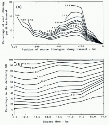
Figure. 11b shows the changing composition of successive sediment packages us they move over point A in Figure. 10 between 11.5 and 15.5 k model years. Note that in the earlier part of this period, far-travelled debris is relatively more important than later, when the site is much nearer the ice margin. The lithological compositon at 15.5 ka represents the lithology over the site immed-iately before deposition begins there. The superimposition of material from successive trajectories, which builds up a till sequence with a vertical lithological gradient, is described later (Fig. 14).

Fig. 12.

The bulk lithological composition in relation to source lithology of the retreat-phase tills deposited during the cycles shown in Figures 7 and 10. Source lithologies are shown along the bottom, 1-19 to the south of the initial final ice divide and −1 to −12 to the north. The bulk composition of the till at any distance from the initial divide is shown in terms of the proortions derived from individual source lithologies. For instance, the till at 400 km contains 45% of lithology 8.25% of lithology 7.18% of lithology 6. etc. Material is transported to the north across the final divide position because of the divide excursion to the south during the glacial maximum (Fig. 10) but it is not transported to the south across the divide. Note that the simplifications inherent in the ice-sheet model overstimate transport distances.

Fig. 14.

Detail of Figure. 13 showing the pattern of till deposition. It shows the progressive accumulation of till (cumulative thickness shown in metres) from the sediment pockages travelling along time-space trajectories 0, 2, 4 and 6 (note that horizontal lines are time lines). At 128 km and 114 km, progressive accumulation of till through time at fixed locations is shown. In these two latter cases, the till builds up in increments derived from successive time-space trajectories. As the lithological composition of succeeding sediment packages along these trajectories changes, so will the accumulating till show vertical changes in lithology. It can he seen that the base of the till accumulating al 144 km (the distal extremity of the indicator source) will contain a greater proportion of the indicator than higher levels, as the trajectory feeding the base has travelled for a longer period, at higher erosion rates, over the indicalor source (see also Fig. 16).

Figure. 12 shows the bulk composition of the retreat-phase till deposited during the glacial cycle illustrated in Figures 7 and 10 in relation in source lithologies. A series of possible source lithologies is shown, lo the south of the initial and final ice divide (1 to 19) and to the north of the divide (−1 to −12). Because of the shift of the divide to the south and then back to the north during the glacial cycle (Fig. 10), debris is carried across the divide to the north but not to the south. For the first 300 km to the south of the final divide, debris is only carried for a small distance beyond its source. Thereafter, an increasing proportion of the till is far-travelled, so that at the furthermost extent of the glacier to the south almost 50% of the till constituents have travelled more than 200 km.

The increase of the mean transport distance shown in Figure. 12 beyond 300-400 km reflects the high values of ice velocity and erosion rate in the outer zone during the ice sheet’s greatest expansion. The presence of lithologies 1. 2 and 3 beyond 400 km, though they are absent between 250 and 400 km, reflects their rapid transport during the growth phase of the ice sheet.

Figures 13 and 14 illustrate the dispersal from a single target in the model illustrated in Figure. 7. Figure. 13 shows a zone 0-250 km south of the final divide during the ice-sheet decay phase. Sediment time-distance trajectories, erosion rates and the outer depositional zone are mapped on to the time-distance diagram. It is assumed that indicator erratic dispersal from a specific source will have taken place during the ice-sheet advance phase but that this will leave only trace quantities in the retreat-phase will be dictated by the furthest extent of the earliest retreat-phase trajectory derived from the source, determined in this case by the time at which the ice divide moved north of the source (Fig. 13). This earliest trajectory transported material about 100 km from the source before ice-sheet margin retreat past this point terminated transport of the debris package. If we consider a later trajectory which crosses the indicator source (e.g. Fig. 13, trajectory O), it will have crossed the source when this coincided with a higher rate of erosion, and when the source was closer to the till which formed at the end of the trajectory, so that indicator erratics were not so diluted by subsequent debris added to the travelling sediment package. Thus, if the concentration of indicator erratics in the retreat-rate till is plotted (Fig. 15), it increases towards the indicator source. In the specific case modelled here, the peak concentration occurs some 10 km south of the source. This reflects the fact that, for this time distante dynamic pattern, the greatest amount of indicator debris is picked up along trajectory 6-7 (Fig. 13) and, although slightly diluted, it still exceeds the proportion picked up along later trajectories. The indicator erratic peak (Fig. 15) can he moved nearer to or further from the source by adjusting the glacier dynamics and the retreat rate. The concentration inevitably falls to the right of the distal extremity of the source (unless there are ice-front oscillations in this zone) as the period during which erosion occurred along any trajectory diminishes to the right of the distal extremity (Fig. 13)

Fig. 13.

Time-distance properties of an ice sheet which control indicator erratic dispersal from a specific source. It shows a detail of the retreat phase of the cycle illustrated in Figures 7 and 10. Erosion rates, time-space debris transport trajectories, movement of the ice divide and the location of the depositional zone are shown. As the ice divide moves north of the indicator source site, material from it begins to be transported south. The intersection of this earliest trajectory with the retreating ice margin determines the maximum extent of dispersal from the source during the retreat phase. Sediment packages along successive trajectories which cross the source (0-6) will contain increasing proportions of the indicator lithology as the decreasing distance between the source and the location of deposition will produce less dilution of indicator erralics in the packages, and the maximum erosion rates occur over the source when trajectories 6 and 7 cross it. This will lead to the train shown in Figures 15 and 16.

Fig. 15.

Average concentration of indicator erratics in the depositional train derived from the indicator source shown in Figure. 13. The earliest trajectory from the source shown in Figure. 14 determines the location of the end of the train, and the peak concentration coincides with the packages deposited from trajectories 6 and 7 (Fig. 13). The length of the train and the location of the peak concentration can be changed by adjusting glacier/till dynamics and the retreat rate.

The pattern shown in Figure. 15 is similar to the classic pattern of indicator-debris decrease in a till down-ice from the indicator source (Reference Shilts and LeggetShilts, 1976). The dispersal distance is, however, typically 2-20 times larger than is normally found in the central area of an ice sheet analogous to the zone modelled in Figure. 15. This does not arise from the theory nor necessarily from the till rheologies used, but from the way in which the simplified ice-sheet model is used to exemplify the theory, by overemphasizing the bed-deformation component of ice-sheet movement. It may also be that the mass balance used lo drive the ice-sheet flow is too large for all ice sheet during its final decay.

It is also possible in reconstruct the distribution of till lithologies from a given Source in a vertical plane parallel to ice flow from the construction shown in Figure. 14. Progressive till accumulation in the depositional zone is shown for a number of debris trajectories. Because of the continuous mixing process referred to above, the debris in transport along a given trajectory in the deposition zone has a constant Composition. However, the till which accumulates at one place does so by deposition from a series of time-distance trajectories. Because debris packages on different trajectories are of different composition, the till accumulating at one point progressively changes composition. The concentration of indicator erratics from the source shown in Figures 13 and 14 along a flow section of the retreat-phase till is shown in Figure. 16. Concentration contours in the till dip in an up-ice direction, as is found in real examples e.g. Reference Kauranne, Salminen and AyräsKauranne and others, 1977).

Fig. 16.

Thickness, composition and isochronous surfaces in the till accumulating between 120 km and 250 km in Figure. 7. The location of the indicator source (Figs 13 and 14) is shown and the concentration of indicator errarics in the till. The concentrations can be derived graphically from Figure. 14. Isochronous surfaces have a lower dip than the compositional anomalies. They reflect a depositional zone which is about 25 km in width.

As noted above, predicted erratic dispersal distances are a consequence of prescribed ice-sheet occupancy times, ice fluxes and till rhcology, and the arbitrary decoupling, in the interests of simplicity, of the ice/till deformation system. Predicted dispersal distances produced by this approach cannot therefore yet be used to test the theory by comparison with observed dispersal distantes. The predicted vertical patterns of erratic distribution in till can, however, be used to test the theory. The theory could then be used to infer aspects of past ice-sheet dynamics by determining the ice-sheet till parameters which produce a good fit to a particular dispersal train.

Isochronous Surfaces in Till

In any depositional system, it is important to understand the pattern of sediment accumulation in time and space. Figure. 7, which shows the sequential evolution of till at a number of sites, and Figure. 14, which shows accumulation of the retreat-phase till in detail, permit us to follow temporal evolution of a till by plotting isochronous surfaces within the till. In both figures, horizontal lines are time lines. Along the 21 ka time line in Figure. 14, for example, deposition was just ceasing al 205 km and just beginning at 180 km, a depositional zone of 25 km extent. The 21 ka isochronous surface within the till is not, however, a straight line from the top of the till at 205 km to its base at 180 km. Near the up-glacier extremity of the depositional zone at 21 ka, initial deposition rates are slow, whilst near its down-glacier extremity, deposition rates are high (Fig. 14). Figure. 16 shows the upwardly convex isochronous surfaces for till produced by the transport trajectories in Figure. 14. It can also be seen from Figure. 16 that isochronous surlaces cut the till-transport trajectories, and thus that the compositional contours in the till will be steeper than isochronous surfaces, reflecting the time-transgressive advance of a compositional wave in the deforming till.

Isochronous surfaces can be complex near to the ice sheet’s maximum extent, or where complex marginal fluctuations have occurred. It can be seen from Figure. 7 that the advance-phase till will have isochronous surfaces along which deposition is initiated at the distal extremity of the zone of deposition (at the point where the glacier transgresses over a site) as it ceases at the proximal extremity. Thus, in contrast lo the retreat-phase till, isochronous surfaces will dip down-glacier from the top of the advance-phase till to its base (Fig. 17). In the terminal zone, where an advance-phase till is preserved below the retreat-phase till, though separated from it by an erosion surface, isochronous surfaces intersect the erosion surface but dip down-glacier in the advance-phase till and up-glacier in the retreat-phase till (Fig. 17). In the extreme terminal zone, where there is a gradation between advance- and retreat-phase tills, isochronous surfaces are parallel.

Fig. 17.

Isochronous surfaces in the till generated as a result of the glacial cycle shown in Figure. 7. (b) is an enlarged version of the lefthand side of (a). The time lines (T₁₀−T₂₃) are in thousands of years after initiation of the glacial cycle. Note that the dip is down-ice in the advance-phase till and up-ice in the retreat phase.

Intra-Till Erosional Surfaces and Boulder Pavements

The theory suggests that, near to the maximum extent of a glacier advance or re-advance, we should expect a zone in which the advance-phase till has been partial eroded before further till is deposited during the retreat phase.

Erosion due to sediment deformation takes place by lowering the interface between the rapidly deforming A horizon and the stable B horizon (Fig. 18b). The uppermost part of the B horizon, as it fails and begins to deform, dilates, takes in further pore water and is reduced in density. The bulk density of the deforming matrix will be much smaller than that of individual clasts. In experiments at Breiðamerkurjökull (Reference Boulton and HindmarshBoulton and Hindmarsh, 1987), matrix bulk density in a sandy till was typically between 0.6 and 0.65 of the clast density. The material was near to the liquid limit and there was therefore a tendency for clasts to sink through the matrix (Reference LawsonLawson, 1982), a tendency counteracted by the mixing induced by frequent folding events us a consequence of the irregularity of the A/B interface.

Fig. 18.

Formation of a boulder pavement in till. (a) Boulder distribution during deposition. Till deposition occurs due to the rise of the interface between the A and B horizons. There is no tendency for boulder concentration at any specific horizon, as all levels in the till have once been at the A/B interface and any our is as likely to have a boulder concentration as any other. (b) Boulder concentration at the descending A/B interface during erosion. As the A/B interface descends around a boulder, the lift force in the relatively low-density deforming horizon may not be enough to move the boulder above the A/B plane. Consequently, boulders hill tend to be concentrated at the interface as it descends. (c) As a phase of deposition succeeds the erosion phase, the A/B interface again begins to rise and a boulder pavement is left marooned in lhe till, marking the lowest level to which the A/B plane descended during erosion. As in (a), there is no tendency for boulder pavements to develop during deposition.

During deposition of till (Fig. 18a), there is no tendency for boulder Concentrations to develop at any specific horizon, as all horizon, have, at some time, coincided with the rising A/B plane. During subsequent erosion due to descent of the A/B interface, whereas we would expect dilatant matrix to move readily into the deforming mass and to be involved in the mixing process of folding, the dense clasts, on being exposed above the descending A/B interface, would resist being drawn into the flow. They would tend to remain immediately above the descending A/B interface, thus concentrating larger clasts from the mobilized till at the A/B interface (Fig. 18b).

It is only where part of the advance-phase till has survived subsequent erosion, such as at about 900 km in Figure. 7b, that a boulder pavement develops (Reference Dreimanis and LeggetDreimanis, 1976). It will be left at the lowest point to which the A/B plane descends. Subsequent deposition during the retreat phase will preserve this erosional interface and its boulder concentration (Fig. 18c).

It is therefore suggested that the intra-till erosional surfaces, such as those shown in Figures 7 and 17, will lend to be marked by boulder pavements. Whether or not this occurs will depend on the matrix/clast density Contrast during deformation and the “lift” forces developed during folding episodes.

It has been suggested by (Reference Boulton and HindmarshBoulton and Hindmarsh 1987; sec Fig. 8-iv) and Reference Boulton and DobbieBoulton and Dobbie (1993) that under certain conditions the A/B interface will be a sliding interface rather than merely a narrow zone of very high shear strain. No matter which of these it is, but particularly in the former case, we might expect some erosion of the top surface of a boulder pavement to be produced by movement of a till slurry over them. If the boulders of the pavement are stable, which they will tend to be if they penetrate beneath the A/B interface, they may acquire a systematic pattern of striation reflecting the direction of till deformation over them. This has been observed from time to time on boulder pavements (Reference ElsonElson, 1957). If boulder pavements are a product of inter-till erosion, lithological contrasts will tend to occur between overlying and underlying tills.

Reference ClarkClark (1991) has suggested that boulder pavements will simply form at the base of a deforming horizon because of sinking through the matrix. I suggest, however, that this will only occur where erosion, which is the source of deformation till, occurs.

Conclusions

• (1) A theory of erosion, transport and deposition is developed for an ice sheet where the dominant mode of transport is by subglacial sediment deformation. The flux of glacially transported sediment is related to the ice flux. It tends to increase distally in the accumulation area and decrease distally in the ablation area. As a consequence, the inner zone of an ice sheet is predominantly one of erosion and the outer zone one of deposition.

• (2) Modelling a simple cycle of growth and decay of an ice sheet with a fixed ice divide shows a resultant pattern of a divide zone wiih little erosion and thin till, an intermediate zone of increasing erosion depth and till thickness and an outer zone of little or zero erosion and large till thicknesses. In the inner and intermediate zone, the resultant till is deposited during the decay phase. In the outer zone. till from the advance phase survives beneath the decay-phase till. There are gradational contacts between the two in the outermost zone, whilst a little further from the outer limit, an erosion zone, which may be marked by a boulder pavement, intervenes between them.

• (3) If ice divides shift during the glacial cycle, earlier tills can be preserved beneath the relatively inactive divide zone. Earlier tills can also be preserved in areas which lay beneath inter-ice-stream ridges, where low ice-flux rates are expected.

• (4) The theory permits the pattern of glacial dispersal of debris to be computed through a glacial cycle. In general, it predicts that the mean derivation distance of till lithologies will tend to increase upwards in any one sequence; that the derivation distance will increase distally; and that sharp contrasts in till lithology will occur across erosional interfaces.

• (5) The depth and pattern of erosion, the thickness, composition and distribution of tills, the strength of lineations and the dispersal of erratics during glacial cycles all depend on both large-scale, climatically determined ice-sheet dynamic properties, and small-scale attributes of the ice-sheet bed. In climatically maritime areas of large vertical mass-balance gradients, the resultant energetic ice sheets will produce more erosion, thicker tills and stronger lineation than in a continental area of smaller mass-balance gradient.

• (6) Extensive subglacial aquifers will tend to drain the glacier bed and inhibit the deformation process, thereby reducing rates of erosion and deposition.

• (7) Fine-grained sediments on the glacier bed will tend to be eroded and transported more readily than coarsegrained sediments and thus contribute preferentially to the resultant till. This process is a principal determinant of till lithology and explains why tills will tend to be enriched in the finer-grained sediments available in the area over which the glacier has expanded.

• (8) Large-scale reconstructions of till-thickness distribution and drift lineation produced during former glacial periods, and large-scale patterns of erratic distribution in tills can be used to reconstruct glacier dynamic history.