


Impact Statement
Stirred tank reactors are used for homogenisation, interphase mass transfer and chemical reactions in numerous industries. Therefore, there is a persistent need for improving their performance. In this sense, one possibility is to work towards more optimal designs. Another is to take full advantage of the current ones. In any case, it is critical to have a better understanding of the flow in stirred tanks, which is quite complex, particularly in the case of turbulence. This paper considers a linear technique (proper orthogonal decomposition) to decompose three-dimensional instantaneous velocity fields obtained from numerical simulations (large-eddy simulations), with the aim of exploring the most energetic motions and related structures (coherent regions in time and/or space). The findings herein can guide future efforts to make the most of the energetic regions in the flow and also provide a basis for more realistic models to address turbulence–fluid-particles (drops and bubbles) interactions.
1. Introduction
Stirred tanks are mechanically agitated vessels, used for mixing enhancement purposes, encountered in almost 25 % of all operations in the process industry (Reference Nikiforaki, Montante, Lee and YianneskisNikiforaki, Montante, Lee, & Yianneskis, 2003). The flow in these devices is known to be complex – having a wide range of temporal and spatial scales – especially in the case of the turbulent regime. In recent years, and as in other turbulent flow problems, there has been an increasing interest in the study of organised flow motions or coherent structures, as a complement to the traditional approach of investigating long-term turbulence statistics.
Coherent structures are regions of space and time (significantly larger than the smallest turbulence scales) within which the flow field has a characteristic coherent pattern (Reference PopePope, 2000). Typically, efforts to isolate coherent structures follow two basic lines of approach (Reference CantwellCantwell, 1981): (i) identification of instantaneous flow structures and (ii) construction of stochastic representations. Approach (i) consists of using various methods to identify discernible flow patterns, e.g. direct flow visualisation, or the isolation of connected regions in the flow where a relevant property (vorticity, for example) is more intense. On the other hand, approach (ii) consists of implementing an eduction technique to obtain representations of the most probable states of the flow according to an applied criterion. A well-known example of approach (ii) is proper orthogonal decomposition (POD).
The POD procedure is also known as Karhunen–Loève expansion or principal components analysis (Reference SirovichSirovich, 1987). In the context of turbulent flows, POD was introduced by Reference LumleyLumley (1967), and was applied for the first time in the study of wall-bounded turbulence (Reference Bakewell and LumleyBakewell & Lumley, 1967). The basic idea behind POD is not complicated. For an ensemble of realisations, one is looking for a set of orthonormal basis vectors which, on average, are the ‘most similar’ (Reference Berkooz, Holmes and LumleyBerkooz, Holmes, & Lumley, 1993) to all members of the ensemble. Such empirical bases are often denoted as POD modes. Subsequently, once the POD modes are found, each realisation may be represented by a (linear) superposition of the deterministic modes modulated by corresponding random, uncorrelated, coefficients. Furthermore, it can be shown – see Reference Holmes, Lumley, Berkooz and RowleyHolmes, Lumley, Berkooz, and Rowley (2012) – that a truncated expansion in terms of ordered POD modes gives a representation that is better than any other linear representation, having the same number of modes, in terms of capturing the energy content. That is, the representation is optimal even with just a few POD modes and not only in an asymptotic sense. In consequence, when considering the POD representation of the velocity field, it is not surprising that some researchers denote the POD modes as characteristic eddies (Reference LumleyLumley, 1970).
During the last two decades or so, the POD procedure has been implemented for the study of stirred tanks in transitional (see e.g. Reference Charalambidou, Micheletti and DucciCharalambidou, Micheletti, & Ducci, 2023; Reference Fan, Sun, Jin, Sun, Zhang, Chen and LiFan et al., 2022; Reference Hasal, Montes, Boisson and FořtHasal, Montes, Boisson, & Fořt, 2000; Reference Raju, Balachandar, Hill and AdrianRaju, Balachandar, Hill, & Adrian, 2005) and turbulent (see e.g. Reference de Lamotte, Delafosse, Calvo and Toyede Lamotte, Delafosse, Calvo, & Toye, 2018; Reference Doulgerakis, Yianneskis and DucciDoulgerakis, Yianneskis, & Ducci, 2011; Reference Hasal, Montes, Boisson and FořtHasal et al., 2000; Reference Moreau and LinéMoreau & Liné, 2006; Reference Raju, Balachandar, Hill and AdrianRaju et al., 2005) flow regimes. Nevertheless, previous works considered two-dimensional velocity fields and it was not until recently that POD analyses and reconstructions based on three-dimensional (3-D) velocity fields have been reported. Reference JanigaJaniga (2019) and Reference Mikhaylov, Rigopoulos and PapadakisMikhaylov, Rigopoulos, and Papadakis (2021, Reference Mikhaylov, Rigopoulos and Papadakis2023a, Reference Mikhaylov, Rigopoulos and Papadakis2023b) considered simulations of unbaffled stirred tanks. Reference JanigaJaniga (2019) performed large-eddy simulation (LES) of the turbulent regime where the flow is agitated with a pitched-blade turbine with three blades. The movement of the propeller was incorporated using the sliding mesh approach (Reference Murthy, Mathur and ChoudhuryMurthy, Mathur, & Choudhury, 1994), and the POD analysis was performed in two different regions of the tank (a per-zone approach). A fixed region was considered to analyse macrostabilities (large-scale, long-lived, quasi-periodic structures; see e.g. Reference Nikiforaki, Montante, Lee and YianneskisNikiforaki et al., 2003), whereas a rotating region was examined to explore the structures related to the periodic passage of the blades, i.e. trailing vortices (counterrotating vortex pairs generated behind the upper and lower edges of each impeller blade; see e.g. Reference Escudié, Bouyer and LinéEscudié, Bouyer, & Liné, 2004; Reference Van't Riet and SmithVan't Riet & Smith, 1975). On the other hand, Reference Mikhaylov, Rigopoulos and PapadakisMikhaylov et al. (2021) and Reference Mikhaylov, Rigopoulos and PapadakisMikhaylov et al. (2023a) performed direct numerical simulations of transitional flow where the rotational motion is induced by a six-blade Rushton turbine. The movement of the impeller was addressed through the frozen motor approach (Reference Luo, Issa and GosmanLuo, Issa, & Gosman, 1994) and the POD technique targeted the reconstruction of trailing vortices based on velocity (Reference Mikhaylov, Rigopoulos and PapadakisMikhaylov et al., 2021) and pressure (Reference Mikhaylov, Rigopoulos and PapadakisMikhaylov et al., 2023a) data from a small number of probing points. After these two works, for the same tank geometry and stirrer, Reference Mikhaylov, Rigopoulos and PapadakisMikhaylov et al. (2023b) performed LES of turbulent flow with the aim of studying and reconstructing macrostabilities from sparse measurements. Interestingly, in this study, the first pair of modes are associated with trailing vortices that appear to form a macrostability as they propagate away from the blades, whilst the second pair of modes are believed to represent the precession of large structures around the impeller shaft. Conversely, there is a single study about POD applied to 3-D velocity fields in baffled stirred tanks. Reference Mayorga, Morchain and LinéMayorga, Morchain, and Liné (2022) considered the turbulent flow in a four-baffled stirred tank operating with a Rushton turbine. In Reference Mayorga, Morchain and LinéMayorga et al. (2022), the turbulent flow is modelled with an unsteady Reynolds-averaged Navier–Stokes method and, as in Reference JanigaJaniga (2019), a sliding mesh approach is used for the propeller. Yet, on the contrary, a global approach is proposed for the POD reconstruction of mean and organised flow motion, the latter due to the periodic passages of the blades in the stirred tank.
Considering the works mentioned previously (Reference JanigaJaniga, 2019; Reference Mayorga, Morchain and LinéMayorga et al., 2022; Reference Mikhaylov, Rigopoulos and PapadakisMikhaylov et al., 2021, Reference Mikhaylov, Rigopoulos and Papadakis2023a, Reference Mikhaylov, Rigopoulos and Papadakis2023b), it is noticeable that the attention given to POD modes other than those related to the mean flow motion, trailing vortices and macroinstabilities has been minor. In a complex flow, the attractiveness of the POD technique resides in its capability for yielding an optimal (linear) stochastic representation of a velocity signal in the sense of capturing, on average, the largest amount of kinetic energy (KE). Therefore, energetic modes associated with turbulent fluctuations and their resulting velocity reconstructions are certainly also worth exploring. Of course, information about the mean flow pattern, trailing vortices and macroinstabilities is still of utmost importance. The mixing efficiency, as well as product quality, are influenced by the flow patterns occurring in the stirred vessel (Reference Chhabra and RichardsonChhabra & Richardson, 2008). Power consumption – perhaps the most important parameter from a practical point of view – is majorly affected by the mean flow (Reference Mikhaylov, Rigopoulos and PapadakisMikhaylov et al., 2023a). In addition, the disruption of trailing vortices also impacts the power consumption by affecting the time-average recirculation pattern on the suction side and leading to a decrease in energy dissipation (Reference Başbuğ, Papadakis and VassilicosBaşbuğ, Papadakis, & Vassilicos, 2018a). Mixing time is affected as well by the disruption of the trailing vortices – due to the changes in the mean flow circulation inside the vessel (Reference Başbuğ, Vassilicos and PapadakisBaşbuğ, Vassilicos, & Papadakis, 2018b) – and by macroinstabilities, when their cores are used for feed insertion (Reference Ducci and YianneskisDucci & Yianneskis, 2007). Furthermore, trailing vortices are also known to provide a source of turbulence (Reference Escudié, Bouyer and LinéEscudié et al., 2004) and to produce regions of high strain in their proximity (Reference Bouremel, Yianneskis and DucciBouremel, Yianneskis, & Ducci, 2009) where mixing could be performed more efficiently.
Keeping in mind Reference Hussain and ReynoldsHussain & Reynolds's (Reference Hussain and Reynolds1970) triple decomposition, the goal of the present paper is to investigate, for a baffled stirred tank and two different fluids, the most energetic POD modes corresponding to mean, organised (periodic) and turbulent motion. Regarding the latter, the idea is to use the higher-order modes to also reconstruct 3-D velocity fields mostly representing the turbulent fluctuations. These approximations to the velocity fluctuations may then be used to explore turbulent structures in the agitated vessel. More specifically, vortical structures are considered and their shape is studied. In the context of stirred tanks, vortices are extremely important due to their role in mixing and possibly in the breakup and coalescence of fluid particles (drops and bubbles) in turbulent dispersions. Indeed, one plausible scenario is that topological changes experienced by the fluid particles are strongly dependent upon the interactions with surrounding swirling-like structures. For instance, a drop embedded into a structure much larger than it may be advected with the structure with little deformation, whilst if the structure is of a comparable size and strong enough to overcome the cohesive forces will cause its breakage into two or more daughter particles. Moreover, not only are the size, intensity and proximity to the fluid particles likely deciding factors but also the shape, number of structures and type of interactions. A droplet squeezed between two corotating structures could be torn apart whereas between two counterrotating ones could be just elongated (Reference Kresta and BrodkeyKresta & Brodkey, 2004). Here, the shape of the structures is crucial since it determines the amount of contact area and how different properties are distributed which, in turn, affects important integral quantities such as circulation (macroscopic measure of rotation). In fact, many phenomenological models for the breakup and coalescence processes (see e.g. Reference Liao and LucasLiao and Lucas (2009, Reference Liao and Lucas2010) and Reference Solsvik, Tangen and JakobsenSolsvik, Tangen, and Jakobsen (2013) for reviews of these models) are based on several simplifications to these factors, including the interaction of fluid particles with structures having matching size and being of spherical shape. In this work, our aim is to address as well how reasonable this last-mentioned assumption is for vortices arising due to the most energetic, POD-reconstructed, velocity fluctuations.
The paper is organised as follows. Section 2 outlines the numerical experiments and the database considered for the analyses. Section 3 summarises the POD procedure and the ‘method of snapshots’ (Reference SirovichSirovich, 1987), which is an alternative and (in general) less computationally expensive method. Section 3 describes as well an objective version of the traditional  $Q$-criterion (Reference Hunt, Wray and MoinHunt, Wray, & Moin, 1988) considered to identify vortical structures. Material objectivity (frame invariance) is a highly desirable property for vortex criteria (Reference Günther, Gross and TheiselGünther, Gross, & Theisel, 2017), especially in case of rotating flows (see Reference Günther, Schulze and TheiselGünther, Schulze, & Theisel, 2016). Next, § 4 presents the modal analysis and the characterisation of the identified vortical structures in terms of their shape. Finally, § 5 provides some concluding remarks.
2. Numerical experiments
To perform POD, a database obtained from LES of an 11 l, baffled stirred tank with a Rushton-type impeller is considered. The simulations were performed using the commercial package Ansys FLUENT (version 19.1, Ansys Inc., Canonsburg, PA). The minimum and maximum grid sizes were set to  $2\times 10^{-4}$ and $4\times 10^{-3}$ m, respectively. Such resolution was deemed adequate for the LES considering that rough estimates – based on isotropic conditions, volume-averaged dissipation rate and turbulent KE – for the Taylor microscale and the Kolmogorov length scale (see e.g. Reference Escudié and LinéEscudié & Liné, 2003; Reference Sharp and AdrianSharp & Adrian, 2001) were mostly within the order of $10^{-4}$– $10^{-3}$ m and of the order of $10^{-5}$ m, respectively. These estimates are for the Newtonian case which is the most restrictive (see next paragraph). The computations were initialised with the results obtained from steady Reynolds-averaged Navier–Stokes simulations, and the volume-averaged torque and turbulent KE were monitored during the LES. Instantaneous realisations (samples) were only taken after reaching statistically stationary conditions.
For the analyses, two test cases are considered. The stirred vessel operates at 800 rpm (impeller frequency  $f_N\approx 13.33$ r.p.s. or Hz), and the working fluid is either water (Newtonian) or a 0.2 wt% carboxymethyl cellulose (CMC) solution presenting shear-thinning behaviour (see e.g. Reference IrgensIrgens, 2014). Information about the tank configuration is given in figure 1 and table 1. A summary of other relevant parameters is presented in table 2. Note that the normalised total sampling time reported in table 2 corresponds to approximately 22.67 cycles of the stirrer. On the other hand, the reported normalised time between collected samples corresponds to a normalised sampling frequency, $f_{sam}/f_N$, of approximately 18.75. Such $f_{sam}$ is suitable for the study of flow structures of intermediate scale taking place close to and at the blade passage frequency, $f_{BPF}=6f_N$ (six times the impeller frequency for a six-bladed disc turbine). Moreover, the total sampling time is also large enough to capture many cycles of these structures and, potentially, even traces of other quasi-periodic, long-lived structures, i.e. macroinstabilities.
Geometrical configuration of the stirred tank considered in the LES: (a) cross-sectional view and (b) top view. The values of the geometrical parameters are given in table 1. The Cartesian coordinate system is shown in blue. Figure adapted from Reference Arosemena, Ali and SolsvikArosemena et al. (2022), copyright 2022 AIP Publishing.

Geometrical details for the stirred tank considered in the LES. The tank diameter  $T=24$ cm. For corresponding schematic representation, see figure 1.

Parameters of the LES. Here W800/C800 refers to simulation case with water/0.2 wt% CMC where the tank operates at  $800$ r.p.m. Time $t_A$ denotes the total sampling time (after discarding the initial transients), $u_{tip}$ is the tip speed of the impeller and $\Delta t$ is the time between the samples. Parameter $Re_{mix}$ is a mixing Reynolds number based on the working fluid density $\rho$, the impeller rotational speed $N$ and diameter $D$, and an apparent fluid viscosity $\mu _a$ for an average strain rate according to the Metzner–Otto correlation for a Rushton-type stirrer (see Reference Metzner and OttoMetzner & Otto, 1957). For water, $\mu _a$ is the dynamic viscosity whereas for the 0.2 wt% CMC case, $\mu _a$ is computed according to the Carreau fluid model (see Reference Arosemena, Ali and SolsvikArosemena et al. (2022) for further details).

For further details about the LES and the test cases, see Reference Arosemena, Ali and SolsvikArosemena et al. (2022).
3. Methods
3.1 The POD procedure and the method of snapshots
The classical POD procedure aims to find a set of optimal basis vectors to represent the flow field data, e.g.  ${\boldsymbol{\mathsf{U}}}\in \mathbb {R}^{n\times m}$, where ${\boldsymbol{\mathsf{U}}}$ denotes a data matrix comprised of instantaneous velocity fields $\boldsymbol {u}$, $n$ is the number of grid points times the number of variables (three in the case of a 3-D velocity field) and $m$ is the number of collected realisations. In other words, one has an extremisation problem resulting in the following eigenvalue formulation (Reference Holmes, Lumley, Berkooz and RowleyHolmes et al., 2012):
 \begin{equation} {\boldsymbol{\mathsf{R}}} {\boldsymbol{\phi}}_{\left(k\right)} = {\lambda}_{\left(k\right)} {\boldsymbol{\phi}}_{\left(k\right)},\quad {\boldsymbol{\phi}}_{\left(k\right)}\in\mathbb{R}^{n\times 1},\enspace \lambda_{\left(1\right)} \geq \cdots\geq \lambda_{\left(n\right)} \geq 0,\enspace k = 1,\ldots,n, \end{equation}
where  ${\boldsymbol{\mathsf{R}}}=\boldsymbol{\mathsf{U}}\boldsymbol{\mathsf{U}}^{\boldsymbol{\mathsf{T}}} \boldsymbol{\mathsf{W}}/m\in \mathbb {R}^{n\times n}$ is the weighted covariance matrix, ${\boldsymbol{\phi}}_{(k)}$ is the set of eigenvectors or POD modes and ${{\lambda }}_{(k)}$ are the corresponding eigenvalues. Note that $\boldsymbol{\mathsf{W}}$ is an $n\times n$ matrix arising after considering the discrete form of the inner product (see e.g. Reference Smith, Moehlis and HolmesSmith, Moehlis, & Holmes, 2005; Reference Taira, Brunton, Dawson, Rowley, Colonius, McKeon and UkeileyTaira et al., 2017) and which accounts for the grid non-uniformity. The optimal linear expansion is then given by
 \begin{equation} \boldsymbol{\mathsf{U}} = \sum_{k = 1}^{n} {\boldsymbol{\phi}}_{\left(k\right)} {{\boldsymbol{a}}}_{\left(k\right)} \approx \sum_{k = 1}^{r} {\boldsymbol{\phi}}_{\left(k\right)} {{\boldsymbol{a}}}_{\left(k\right)},\quad {{\boldsymbol{a}}}_{\left(k\right)}\in\mathbb{R}^{1\times m},\enspace r< n, \end{equation}
where the set of uncorrelated temporal coefficients  ${{\boldsymbol{a}}}_{(k)}$ is found by projecting the input data into the $k$-mode. Usually, a satisfactory upper bound $r$ for the truncated series is much less than the total number of modes $n$.
$n$.
An issue with the classical POD method is that for a very large  $n$, solving the eigenvalue problem becomes impractical and sometimes even not possible. An alternative approach is the method of snapshots proposed by Reference SirovichSirovich (1987). The basic idea is that instead of having a decomposition involving deterministic spatial modes and random time coefficients, one may have a decomposition in terms of deterministic temporal modes with random spatial coefficients (Reference WeissWeiss, 2019). This is computationally advantageous since, typically, $m<< n$ and the resulting eigenvalue problem involves a matrix of size $m\times m$ rather than of size $n \times n$. Of course, the method does not provide a full POD representation, and to be successful the chosen realisations must be representative of the flow statistics (Reference JiménezJiménez, 2018). In any case, once the reduced eigenvalue problem is solved, one can recover the leading spatial POD modes through a transformation as shown next.
In the method of snapshots, the resulting eigenvalue problem is as follows (Reference Holmes, Lumley, Berkooz and RowleyHolmes et al., 2012):
 \begin{equation} \hat{\boldsymbol{\mathsf{R}}} \hat{\boldsymbol{\phi}}_{\left(k\right)} = {\lambda}_{\left(k\right)} \hat{\boldsymbol{\phi}}_{\left(k\right)},\quad \hat{\boldsymbol{\phi}}_{\left(k\right)}\in\mathbb{R}^{m\times 1},\enspace \lambda_{\left(1\right)} \geq \cdots\geq \lambda_{\left(m\right)}\geq 0,\enspace k = 1,\ldots,m, \end{equation}
where  $\hat {\boldsymbol{\mathsf{R}}}=\boldsymbol{\mathsf{U}}^{\boldsymbol{\mathsf{T}}} \boldsymbol{\mathsf{W}}\boldsymbol{\mathsf{U}}/m\in \mathbb {R}^{m\times m}$ is the reduced matrix, sharing the same leading eigenvalues with $\boldsymbol{\mathsf{R}}$ (Reference Taira, Brunton, Dawson, Rowley, Colonius, McKeon and UkeileyTaira et al., 2017), and $\hat {\boldsymbol{\phi}}_{(k)}$ is the temporal eigenvector. Thereafter, the spatial modes are recovered from
 \begin{equation} {\boldsymbol{\phi}}_{\left(k\right)} = \boldsymbol{\mathsf{U}}\hat{\boldsymbol{\phi}}_{\left(k\right)} \frac{1}{m^{1/2} {\lambda}^{1/2}_{\left(k\right)}} \in\mathbb{R}^{n\times 1},\enspace k = 1,\ldots,m, \end{equation}
which is obtained by considering the singular value decomposition (see e.g. Reference Press, Teukolsky, Vetterling and FlanneryPress, Teukolsky, Vetterling, & Flannery, 2007) of  $\boldsymbol{\mathsf{W}}^{1/2}\boldsymbol{\mathsf{U}}/m^{1/2}$.
3.2 An objective version of the  $Q$-criterion

Swirling-like structures or vortices are the ‘sinews and muscles of fluid motion’ (Reference KüchemannKüchemann, 1965). This is even more so when the flow is turbulent and/or rotational. Over the years, many vortex identification methods have been proposed (see Reference EppsEpps (2017) for a recent review). The  $Q$-criterion (Reference Hunt, Wray and MoinHunt et al., 1988) is among the most popular ones. In this method, a vortex is a local region in which there is an excess of rotation rate relative to the strain rate (Reference Chakraborty, Balachandar and AdrianChakraborty, Balachandar, & Adrian, 2005). Nevertheless, the $Q$-criterion, as other Galilean-invariant methods such as the $\varDelta$-criterion (Reference Chong, Perry and CantwellChong, Perry, & Cantwell, 1990) or the $\lambda _2$-criterion (Reference Jeong and HussainJeong & Hussain, 1995), has an important shortcoming: it is not objective. That is, rotational invariance, an essential feature for rotating flows, it is not fulfilled (see Reference HallerHaller, 2005). In this respect, Reference HallerHaller (2021) remarked that these local vortex criteria may effectively be objectivised by replacing the spin/rotation rate tensor by a spin-deviation tensor. The spin-deviation tensor is defined as the difference between the original rotation rate tensor and its instantaneous spatial average (see Reference Haller, Hadjighasem, Farazmand and HuhnHaller, Hadjighasem, Farazmand, & Huhn, 2016). This procedure was proposed and implemented by Reference Liu, Gao and LiuLiu, Gao, and Liu (2019a) and Reference Liu, Gao, Wang and LiuLiu, Gao, Wang, and Liu (2019b) to objectivise the Rortex criterion (Reference Liu, Gao, Tian and DongLiu, Gao, Tian, & Dong, 2018; Reference Tian, Gao, Dong and LiuTian, Gao, Dong, & Liu, 2018) and the omega method (Reference Liu, Wang, Yang and DuanLiu, Wang, Yang, & Duan, 2016). The same procedure has also been implemented by Reference Arosemena, Ali and SolsvikArosemena et al. (2022) to objectivise the $Q$-criterion, and it may be summarised as follows.
First, the spin-deviation tensor is computed as
 \begin{equation} {\boldsymbol\varOmega_{{\star}}} = {\boldsymbol\varOmega}-\left\langle{\boldsymbol\varOmega}\right\rangle, \end{equation}
where  $\boldsymbol \varOmega =\frac {1}{2} [\boldsymbol \nabla {\boldsymbol {u}} -(\boldsymbol \nabla {\boldsymbol {u}})^{\rm T}]$ is the spin/rotation rate tensor and $\left \langle {\boldsymbol \varOmega }\right \rangle (t) =({1}/{\mathcal {V}})\int _{\mathcal {V}}^{} \boldsymbol \varOmega \,\mathrm d \mathcal {V}$ is the instantaneous spatial average of $\boldsymbol \varOmega$ over the full flow domain $\mathcal {V}$.
Next, the  $Q$-criterion is reformulated as
 \begin{equation} Q_{{\star}} = \tfrac{1}{2}\left[\left|\boldsymbol\varOmega_{{\star}}\right|^2 - \left|\boldsymbol{\mathsf{S}}\right|^2\right], \end{equation}
which is objective (not observer-dependent). Here  $\boldsymbol{\mathsf{S}} = \frac {1}{2} [\boldsymbol \nabla {\boldsymbol {u}} +(\boldsymbol \nabla {\boldsymbol {u}})^{\rm T}]$ is the strain rate tensor.
4. Results
Before discussing the results, it is important to clarify some points about the input data. The impeller movement in the LES is implemented by means of the sliding mesh approach. Therefore, regardless of having an inertial or a rotational frame of reference, part of the mesh is moving as the simulations proceed. In such cases, to date, the following strategies have been implemented: (i) the POD method is applied in a per-zone manner where different modes and coefficients are found for the stationary and rotating domains or zones (Reference JanigaJaniga, 2019) and (ii) the POD method is applied in a global manner considering the two zones altogether (Reference Mayorga, Morchain and LinéMayorga et al., 2022). Both strategies are feasible for POD reconstruction of the velocity field yet pose some issues for the analysis of the modes. In the case of the per-zone treatment, the connection between modes in the two zones and their energy content is rather ambiguous. On the other hand, with respect to the global treatment, direct physical interpretation of the POD modes is not possible since the modes are referenced to the elements of the mesh (cells), the positions of which change from time step to time step in the rotating zone.
In this work, instead, the flow-field data are interpolated to a fixed set of points through Sibson (natural neighbour) interpolation (Reference SibsonSibson, 1981). This interpolation scheme is more computationally expensive than others; however, it is known to work well with scattered data (Reference Park, Linsen, Kreylos, Owens and HamannPark, Linsen, Kreylos, Owens, & Hamann, 2006). The query points are set to those of the mesh of the first saved snapshot for the cases outlined in table 2. Here, as with any interpolation method, the issue is how well the interpolated data approximate the original values and may reflect the actual physical process. Appendix A presents a comparison between a randomly selected velocity field for case W800 and its natural neighbour interpolation.
4.1 The POD modal analysis
The amount of KE contributed by each POD mode is found in the corresponding eigenvalue. Figure 2(a) displays the energy contained in the  $k$-mode normalised by the energy contained in all modes. Mode 1 contains most of the total energy ( ${\approx }$60 %–70 %) followed by modes 2 and 3 with very similar energy levels ( ${\approx }5\,\%$). In comparison, the amount of energy in the remaining modes is fairly small (less than $1$% for $k>6$). From figure 2(a) one can also observe that the decay of energy is slow, especially as the theoretical estimate for the inertial subrange (Reference Knight and SirovichKnight & Sirovich, 1990) is approached. Moreover and as expected, this behaviour is more prominent for the higher-Reynolds-number case, i.e. W800. This is more clearly seen in figure 2(b) where the cumulative percentage of total KE is shown. It is also worth noting that at least 95 % of the total KE is captured once about a third of the total number of modes $m$ is considered. Lastly, regarding the sensitivity of the results to the number of considered snapshots, Appendix B compares the fraction of total KE for case W800 – presented in figure 2(a) – with the fraction when the number of snapshots is doubled.
The KE content in POD modes: (a) fraction of total KE versus mode number  $k$ and (b) percentage cumulative amount of KE versus $k/m$. Total number of modes, $m=426$. Colours black and red correspond to cases W800 and C800, respectively. See table 2. In (a), the dotted line represents the $-11/9$ power law (Reference Knight and SirovichKnight & Sirovich, 1990).

In the following, the most energetic modes and their corresponding temporal coefficients are discussed.
Mode 1
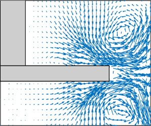
Mode 1 (denoted as the zeroth mode by some researchers) is probably representing the mean flow. This is a classical result when POD is applied to the instantaneous velocity fields (Reference Moreau and LinéMoreau & Liné, 2006). Figure 3 depicts the first eigenvector at selected planes for cases W800 and C800. Figure 3(a,b) shows the  $y,z$ components at $x/T=0$, a cross-section between two baffles, whilst figure 3(c,d) shows the $x,y$ components at $z/T\approx 0.4$, a horizontal plane above the impeller. From figure 3(a,b), one can see the impeller stream and the lower and upper circulation loops. On the other hand, from figure 3(c,d), one can discern the expected effect of using vertical baffles; no gross vortexing is taking place and counterrotating structures – with respect to the rotating direction of the impeller – are appearing behind the baffles. All these patterns are typical of the mean flow for the configuration considered (see e.g Reference Chhabra and RichardsonChhabra & Richardson, 2008). Furthermore, as reported in previous studies (see e.g. Reference de Lamotte, Delafosse, Calvo and Toyede Lamotte et al., 2018), the temporal coefficient for mode 1 is seemly a constant which is being superimposed by small-amplitude, higher-frequency signals. See temporal signal in figure 4(a), displayed only for $t/(T/u_{tip}) \in [0,1]$, and the corresponding power spectral density (PSD) in figure 4(b). As seen from the PSD, aside from the main peak at $f/f_N=0$, there are two other, less noticeable, peaks: one at $f_{BPF}$ and another at its nearest overtone. Note that the latter is being masked due to the considered sampling frequency: $|2f_{BPF}- (\mathcal {N} f_{sam})|/f_N \approx 6.75$, where $(\mathcal {N} f_{sam})$ is the integer multiple of $f_{sam}$ closest to the frequency of interest, $2f_{BPF}$.
Visualisation of POD mode 1 in (a,b) a vertical plane between two baffles at  $x/T=0$ and (c,d) a horizontal plane above the impeller at $z/T\approx 0.4$. In (c,d), the blue arrow indicates the rotating direction of the stirred vessel. Colours black and red correspond to cases W800 and C800, respectively. See table 2.

Temporal coefficient of POD mode 1: (a) normalised temporal coefficient and (b) PSD corresponding to the normalised coefficient. Here,  $f_N$ represents the impeller frequency in revolutions per second. Colours black and red correspond to cases W800 and C800, respectively. See table 2.

It is also interesting to note that there are some differences in the first POD mode of two fluid cases. Compared with the Newtonian fluid case, there are more quasi-stagnant regions, an overall attenuation of the circulation loops and the structures behind the baffles and more asymmetry below the impeller for the shear-thinning fluid. These factors suggest poorer macromixing for case C800, especially in regions away from the impeller.
Modes 2 and 3
Modes 2 and 3 are probably coupled – as mentioned previously in this section, these modes have nearly identical energy content – and represent organised motion due to the periodic passage of the blades, namely trailing vortices as reported in previous works (see e.g. Reference Gabelle, Morchain and LinéGabelle, Morchain, & Liné, 2017; Reference Liné, Gabelle, Morchain, Anne-Archard and AugierLiné, Gabelle, Morchain, Anne-Archard, & Augier, 2013). Figure 5(a–d) shows the  $y,z$ components of the second and third eigenvectors at $x/T=0$ for cases W800 and C800. As can be seen and as expected in the case of trailing vortices, modes 2 and 3 reveal swirling-like, counterrotating patterns exhibiting symmetry with respect to the plane of the impeller ( $z=C$), albeit these are not as pronounced for the shear-thinning fluid case when compared with the Newtonian case. In addition, the analysis of the temporal coefficients corresponding to modes 2 and 3 evidences their coupled periodic nature. Figure 6(a), presenting the normalised temporal coefficients for $t/(T/u_{tip}) \in [0,1]$, allows one to note an apparent out-of-phase, sinusoidal-like behaviour in the signals. Moreover, as displayed in figure 6(b), their corresponding PSDs are peaking at the blade passage frequency which emphasises the connection between modes 2 and 3 and the periodic motion due to the passages of the blades. Here, note as well there is a second, barely noticeable, peak at $f/f_N \approx 6.75$. As commented before while discussing the temporal coefficient for POD mode 1, this peak happens at the nearest overtone of $f_{BPF}$ with aliasing due to the considered $f_{sam}$ and corresponds to a superimposed, small-amplitude, signal.
Visualisation of POD modes 2 and 3 in a vertical plane between two baffles at  $x/T=0$ and in the vicinity of the impeller: (a,b) mode 2 and (c,d) mode 3. Colours black and red correspond to cases W800 and C800, respectively. See table 2.

Temporal coefficients of POD modes 2 and 3: (a) normalised temporal coefficients, (b) PSD corresponding to the normalised coefficients and (c) phase portrait of the normalised coefficients. In (a,b), continuous and dotted line styles are used for normalised  $a_{(2)}$ and $a_{(3)}$, respectively. In (c), the continuous line represents the unitary ellipse, and to avoid excessive clustering not all data points are displayed. Here, $f_N$ represents the impeller frequency in revolutions per second. Colours black and red correspond to cases W800 and C800, respectively. See table 2.

Another tool to highlight the harmonic coupling between the modes is the cross-plotting of their temporal coefficients (Reference van Oudheusden, Scarano, van Hinsberg and Wattvan Oudheusden, Scarano, van Hinsberg, & Watt, 2005). This is done in figure 6(c) and as can be seen, although the coefficients are statistically uncorrelated, they are not independent and instead are scattered around an ellipse. This is typical of sinusoidal signals out of phase.
Modes 4 to 11
The POD modes 4 to 11 are probably representing either complex harmonic motion linked to the trailing vortices, or a macroinstability. Previous investigations of stirred tanks have shown that modes following modes 2 and 3 may also exhibit counterrotating structures that are almost symmetric with respect to  $z=C$ (see e.g. Reference Gabelle, Morchain and LinéGabelle et al., 2017; Reference Liné, Gabelle, Morchain, Anne-Archard and AugierLiné et al., 2013). Moreover, together with modes 2 and 3, these structures depict a convective pattern resembling the vortex shedding behind bluff bodies reported in many works (Reference Liné, Gabelle, Morchain, Anne-Archard and AugierLiné et al., 2013). Meanwhile, depending on the total sampling time (here $t_A$; see table 2), it is possible that the modes following modes 2 and 3 are representing a macroinstability (see e.g. Reference Doulgerakis, Yianneskis and DucciDoulgerakis, Yianneskis, & Ducci, 2009).
In the following and to shorten the discussion, the visualisation of all these POD modes (4 to 11) is not shown nor the time evolution of their corresponding coefficients. Instead, here the phase portrait of the coefficients of these modes with  $a_{(3)}$ are investigated to also gain insight into the modes. In the case of periodic vortex shedding, $a_{(3)}$ would be one of the basic harmonics. From figures 7(a)–(h), it is clear that there is some relation between $a_{(3)}$ and the coefficients corresponding to modes 4, 5, 7, 8 and 9 in case W800 and those corresponding to modes 5, 6, 8 and 9 in case C800. The displayed patterns are similar to Lissajous curves which, indeed, suggests complex harmonic behaviour. At this point, it is worth mentioning that (in general) the POD technique is not suitable for isolating structural coherence based on observations about the temporal coefficients, since a given modulated POD mode may encompass different signals and physical phenomena. Therefore, other statistical techniques such as dynamic mode decomposition (see Reference SchmidSchmid, 2010) are preferred when one is interested in the ‘best fit’ for approximating the dynamics of the data. Nevertheless, for periodic and convective phenomena (as in the case of vortex shedding), it is known that both linear decompositions (POD and dynamic mode decomposition) yield remarkably similar structures (Reference Schmid, Violato and ScaranoSchmid, Violato, & Scarano, 2012).
Phase portrait of normalised coefficients, series of mode 3 and (a) mode 4 coefficients, (b) mode 5 coefficients, (c) mode 6 coefficients, (d) mode 7 coefficients, (e) mode 8 coefficients, ( f) mode 9 coefficients, (g) mode 10 coefficients and (h) mode 11 coefficients. Colours black and red correspond to cases W800 and C800, respectively. See table 2.

On the other hand, regarding the remaining temporal coefficients –  $a_{(6)}, a_{(10)}$ and $a_{(11)}$ for W800, and $a_{(4)}, a_{(7)}, a_{(10)}$ and $a_{(11)}$ for C800 – there is no distinctive relation between them and $a_{(3)}$. Besides, when considering the time evolution of these coefficients, an exceedingly long signal is uncovered (see figure 8a,b). Macroinstabilties are large temporal and spatial fluctuations of the flow (Reference Galletti, Paglianti and YianneskisGalletti, Paglianti, & Yianneskis, 2005) arising due to two distinct mechanisms: (i) precessional vortex motion around the shaft (see e.g. Reference Nikiforaki, Montante, Lee and YianneskisNikiforaki et al., 2003) and (ii) the impingement of the jet-like discharge stream on the vessel boundaries (see e.g. Reference Roussinova, Kresta and WeetmanRoussinova, Kresta, & Weetman, 2003). In the turbulent flow regime, the precessional macroinstabilities result in a characteristic frequency which is smaller than the characteristic frequency of the jet-impingement macroinstabilities by an order of magnitude. The frequency of the precessional macroinstabilities is also smaller than the characteristic frequency for trailing vortices by two orders of magnitude (Reference Doulgerakis, Yianneskis and DucciDoulgerakis et al., 2009). In consequence, the behaviour for the remaining temporal coefficients is likely reflecting the presence of precessional macroinstabilities in the flow. Figure 8(c,d) displays the $x,y$ components of the sixth and first eigenvectors at $z/T\approx 0.4$ for case W800, respectively. The former shows precessional patterns around the shaft (see blue boxes in figure 8c).
Traces about precessional macroinstabilities, POD mode 6 for W800 and POD mode 4 for C800: (a) normalised temporal coefficients, (b) PSD corresponding to the normalised coefficients, (c) visualisation of mode 6 at  $z/T\approx 0.4$ and (d) visualisation mode 1 at $z/T\approx 0.4$. In (c), the blue boxes mark regions with precessional patterns. In (d), the blue arrow indicates the rotating direction of the stirred vessel. Here, $f_N$ represents the impeller frequency in revolutions per second. Colours black and red correspond to cases W800 and C800, respectively. See table 2.

Lastly, it is important to stress the limitation of our data in terms of characterising precessional macroinstabilities. For the proper study of these periodic or quasi-periodic motions, one requires the recording of at least some full cycles to minimise statistical errors. For example, Reference Ducci and YianneskisDucci and Yianneskis (2007) considered four sets of data corresponding to the same experiment where, for each set, a complete cycle was recorded. Additionally, and with the purpose of capturing at least one full cycle of the precessional motion, the temporal behaviour of  $a_{(6)}$ for case W800 when $t_A$ is doubled is considered as well. See appendix C.
Higher modes
The higher modes involve the higher-order harmonics of the organised motions discussed thus far as well as the turbulent fluctuations. This makes the analysis of the subsequent POD modes increasingly challenging since every mode now has signals with several frequencies, and possibly involves multiple physical phenomena. See figure 9.
The PSD corresponding to the normalised coefficient for mode 100. Here,  $f_N$ represents the impeller frequency in revolutions per second. Colours black and red correspond to cases W800 and C800, respectively. See table 2.

In the remaining part of the paper, our attention is redirected to the identification of vortical structures and their morphological characterisation. The vortex detection is based upon reconstructed 3-D velocity fields consisting only of the most energetic higher POD modes. Expressed in a different manner, at a given time  $t$,
$t$,  $\boldsymbol{u}$ may be approximated as
 \begin{equation} {\boldsymbol{u}} \approx \sum_{k = 1}^{r} {a}_{\left(k\right)}{\boldsymbol{\phi}}_{\left(k\right)} \equiv \underbrace{{a}_{\left(1\right)}{\boldsymbol{\phi}}_{\left(1\right)}}_{{({\rm i})}} + \underbrace{\sum_{k = {2}}^{11} {a}_{\left(k\right)}{\boldsymbol{\phi}}_{\left(k\right)}}_{{({\rm ii})}} + \underbrace{\sum_{k = 12}^{r} {a}_{\left(k\right)}{\boldsymbol{\phi}}_{\left(k\right)}}_{{({\rm iii})}}, \end{equation}
and the identification of vortices is based on term (iii). Considering the observations made through § 4, terms (i), (ii) and (iii) of (4.1) seem to represent (for the most part): the mean, periodic and fluctuating components of  $\boldsymbol{u}$ according to Reference Hussain and ReynoldsHussain & Reynolds's (Reference Hussain and Reynolds1970) triple decomposition. Here, the upper limit $r$ is set to capture (at least) $\approx$95 % of the total KE. Thus, the POD reconstruction is truncated at mode 130 which corresponds to $k/m \approx 0.3$ (see figure 2b). The reasoning for truncating the linear expansion at $r=130$ is that within this range a significant amount of KE has already been captured and afterwards, the decay in the energy content is even slower. For example, for case W800 one captures 99 % of the total energy content only after keeping more than the first 300 modes. Indeed, one of the weaknesses of POD is that it is not always clear how many POD modes should be kept, and there are many different truncation criteria (Reference Taira, Brunton, Dawson, Rowley, Colonius, McKeon and UkeileyTaira et al., 2017).
4.2 Vortical structures
The identification and morphological characterisation of vortices related to turbulence proceed as follows.
(i) The vortex criterion is computed. At a given instant, based on the approximation to the fluctuating velocity field, i.e. term (iii) of (4.1), the 3-D
$Q_{\star }$ field is computed according to (3.6).(ii) The vortex criterion is normalised to account for inhomogeneity in the flow. The 3-D
$Q_{\star }$ field is normalised by its root mean square. The idea of using a statistical indicator of the turbulent structure concept to account for inhomogeneity in the flow started with Reference Nagaosa and HandlerNagaosa and Handler (2003) and has been implemented in several works (see e.g. Reference Arosemena, Andersson, Andersson and SolsvikArosemena, Andersson, Andersson, & Solsvik, 2021; Reference del Álamo, Jiménez, Zandonade and Moserdel Álamo, Jiménez, Zandonade, & Moser, 2006; Reference Hwang and SungHwang & Sung, 2018; Reference Lozano-Durán, Flores and JiménezLozano-Durán, Flores, & Jiménez, 2012).(iii) The normalised criterion is thresholded to identify the vortical structures. Regions of connected grid points where the normalised
$Q_{\star }$-criterion is ${\geq }1$ are recognised as individual vortices. Here, connectivity is defined by the six orthogonal nearest neighbours of each grid point and the threshold is chosen considering the percolation crisis analysis performed by Reference Arosemena, Ali and SolsvikArosemena et al. (2022). Also, it is worth mentioning that as in Reference Arosemena, Ali and SolsvikArosemena et al. (2022) and due to the computational cost, a sensitivity analysis to the threshold selected is not performed. Nonetheless, based on previous studies (see e.g. Reference Arosemena, Andersson, Andersson and SolsvikArosemena et al., 2021; Reference Cheng, Li, Lozano-Durán and LiuCheng, Li, Lozano-Durán, & Liu, 2020) and for threshold values larger than that where the percolation transition occurs, it is deemed probable that consistent trends in the results will be observed when changing the threshold value to another one differing by less than an order of magnitude.(iv) The identified vortices are characterised according to statistics of shape-related parameters. Here, the shape of a vortical structure is determined by its maximum projection sphericity
$\varPhi _p=[d_S^2/(d_L d_I)]^{1/3}$ (Reference Sneed and FolkSneed & Folk, 1958), and its elongation $E=d_I/d_L$ and flatness $F=d_S/d_I$ parameters (Reference ZinggZingg, 1935). Here $\varPhi _p$ represents the ratio of maximum projection area of a sphere having the same volume as the structure to the maximum projection area of the structure. Thus, $\varPhi _p$ has a maximum of $1$ for perfect spheres. On the other hand, the two aspect ratios ($F,E$) can be used to classify a structure in terms of its shape (see figure 10). Note that $d_S$, $d_I$ and $d_L$ are the shortest, intermediate and largest lengths of the oriented bounding box of a given structure. The boxes are computed by principal components analysis (see e.g. Reference JolliffeJolliffe, 2002).


Reference ZinggZingg's (Reference Zingg1935) diagram for shape classification of objects according to their elongation  $E$ and flatness $F$ parameters. Corners also illustrate extreme cases discussed in Reference Moisy and JiménezMoisy and Jiménez (2004): ribbons $(0,0)$, sheets $(0,1)$, tubes $(1,0)$ and spheres $(1,1)$. Reprinted from Reference Arosemena, Ali and SolsvikArosemena et al. (2022), with permission of AIP Publishing.

Figures 11(a) and 11(b) display the vortical structures identified by the above procedure for cases W800 and C800, respectively. The rendering takes place in the vicinity of the impeller (not shown in the figure) and for an instantaneous POD reconstruction based on term (iii) of (4.1). As can be seen, the vortices visually appear mostly as tubular structures. It is also interesting to note that the population of structures diminishes for the 0.2 wt% CMC case, as expected for the case having a lower Reynolds number and exhibiting shear-thinning fluid behaviour.
Vortical structures based on POD reconstruction to approximate the fluctuating velocity field, and statistics of shape-related parameters. Isosurfaces of normalised  $Q_{\star }$-criterion $=1$ in the vicinity of the impeller, at a given instant, and for cases (a) W800 and (b) C800. Plots of (c) CDF $(\varPhi _p)$ and (d) JCDF $(F,E)$. In (c,d), continuous and dotted line styles correspond to the data of this work and that of Reference Arosemena, Ali and SolsvikArosemena et al. (2022), whilst colours black and red correspond to cases W800 and C800, respectively. See table 2. Additionally, in (c), the dashed blue line marks CDF $(\varPhi _p)=0.9$, whereas in (d), the blue lines mark the limits for shape classification (see figure 10). Also, in (d), the levels represented contain 99 %, 70 % and 30 % of the data.

Regarding the shape-related parameters, figures 11(c) and 11(d) show the cumulative distribution function (CDF) of  $\varPhi _p$ and the joint CDF (JCDF) of $F$ and $E$, respectively, for cases W800 and C800. Figure 11(c,d) also shows the results of Reference Arosemena, Ali and SolsvikArosemena et al. (2022). As seen from figure 11(c), the probability of the identified vortices being non-spherical is above 90 %; i.e. CDF $(\varPhi _p \leq 0.9)>0.9$ for both cases. This result is larger than CDF $(\varPhi _p \leq 0.9)\approx 0.8$ reported by Reference Arosemena, Ali and SolsvikArosemena et al. (2022) where the identification of vortices is based upon the instantaneous velocity field, instead of a POD reconstruction for the fluctuating velocity component. In addition, figure 11(d) reveals that about 70 % of identified structures are likely to fall into the compact and prolate categories whereas just 30 % of them fall into the compact category alone. This result is consistent with the finding of Reference Arosemena, Ali and SolsvikArosemena et al. (2022), albeit in the latter the contour corresponding to 30 % of the data is slightly closer to the limit for perfect spheres (see figure 10). It is also interesting to observe that the contours of JCDF $(F,E)$ capturing 70 % and 30 % of the data are for a very narrow range of large $F$ values, i.e. $0.8\leq F\leq 1$ and $0.9\leq F\leq 1$, respectively. This finding further strengthens the argument in favour of tube-like vortices of different lengths being detected, instead of spherical ones.
5. Concluding remarks
In this work, POD is performed over instantaneous velocity fields obtained from the LES of an 11 l, baffled, stirred tank operating with a Rushton-type impeller at 800 r.p.m., and where the working fluid is either water or a 0.2 wt% CMC solution (Reference Arosemena, Ali and SolsvikArosemena et al., 2022). The most energetic modes and their corresponding temporal coefficients are investigated. In addition, a POD reconstruction of the higher modes is carried out with the purpose of approximating the fluctuating velocity field and subsequently to explore the shape of vortices related to turbulence in the stirred vessel. Vortical structures are extremely important because of their role in mixing, and (potentially) in the breakup and coalescence of dispersed fluid particles. More specifically, the focus in their morphological characterisation is due to the fact that many phenomenological models for the breakage and coalescence of fluid particles (see e.g. Reference Liao and LucasLiao & Lucas, 2009, Reference Liao and Lucas2010; Reference Solsvik, Tangen and JakobsenSolsvik et al., 2013) are based on several assumptions, including their interaction with vortices having comparable size and being of spherical shape. The identification of vortical structures is achieved through an objective version of the traditional  $Q$-criterion (Reference Hunt, Wray and MoinHunt et al., 1988) which is normalised to also take into account the inhomogeneity in the rotating flow. On the other hand, the morphological classification of the identified structures is made thanks to statistics of their shape-related parameters, maximum projection sphericity and aspect ratios.
Findings of this paper include the following:
(i) It seems promising to implement the POD technique with the purpose of decomposing a 3-D flow field into its mean, and most energetic periodic and fluctuating components according to Reference Hussain and ReynoldsHussain & Reynolds's (Reference Hussain and Reynolds1970) triple decomposition.
(ii) Vortices associated with the fluctuating velocity field are mostly tubular structures.
Finding (i) appears to be valid regardless of the working fluid rheology, consistent with earlier POD analyses based on two-dimensional velocity fields (Reference Gabelle, Morchain, Anne-Archard, Augier and LinéGabelle, Morchain, Anne-Archard, Augier, & Liné, 2013; Reference Liné, Gabelle, Morchain, Anne-Archard and AugierLiné et al., 2013). Likewise, as recognised by Reference Moreau and LinéMoreau and Liné (2006), finding (i) signifies that one would be able to get the periodic component of the flow without the necessity of phased measurements. More importantly, this finding opens the window for reduced-order modelling of the organised structures arising due to periodic motions in the tank: trailing vortices and macroinstabilities. Previous works have considered low-order representations for these organised motions by approximating the corresponding temporal coefficients with sinusoidal functions (Reference Doulgerakis, Yianneskis and DucciDoulgerakis et al. (2009); Reference Ducci, Doulgerakis and YianneskisDucci, Doulgerakis, and Yianneskis (2008), Reference Doulgerakis, Yianneskis and DucciDoulgerakis et al. (2011) and Reference Gabelle, Morchain, Anne-Archard, Augier and LinéGabelle et al. (2013), to list a few). However, more generally, one can do a Galerkin projection of the momentum equation onto these POD modes to obtain a low-dimensional model for their coefficients (see e.g. Reference Smith, Moehlis and HolmesSmith et al., 2005). Once the reduced-order model is solved, it would then be possible to predict the dynamical behaviour of these periodic structures, and thus better use these highly energetic regions for purposes such as mixing enhancement. The advantage of following the more general approach is that one is not restricted to simple periodic motion. Meanwhile, finding (ii) suggests that as starting point for the modelling of breakage and coalescence of fluid particles in stirred tanks and based on their interaction with vortices, it is more reasonable to assume that the latter are cylindrical structures rather than spherical. Moreover, this observation is more in line with our understanding about vortices in turbulent flows (see e.g. Reference DavidsonDavidson (2015), § 5.3). Lastly, through this work and as expected, an overall attenuation of the swirling-like motions (e.g. circulation loops, trailing vortices and vortical structures associated with turbulence) is observed with shear-thinning rheology compared with the Newtonian case.
Finally, it is worth mentioning some limitations of the present investigation. Firstly, since POD is performed over data obtained from LES, none of the higher-order modes are representative of the dissipative scales. Information about the small-scale motions would be particularly useful for improvement of chemically reactive systems and mass transfer. Secondly, the different periodic motions in the tank present different time scales and for proper characterisation of some of them one may require larger simulation times and a complementary dataset with samples collected using a smaller sampling frequency. For example, precessional macroinstabilities in the turbulent regime have a normalised frequency of  $f/f_N\approx 0.02$ (Reference Nikiforaki, Montante, Lee and YianneskisNikiforaki et al., 2003) which is about 300 times smaller than that characteristic of the trailing vortices, i.e. $f/f_N\approx 6$. Thirdly, the standard POD does not ensure temporal coherence and, as seen in § 4.1, it may result in temporal signals with mixed frequencies. This is obviously problematic when considering higher-order modes since it is difficult to separate the higher-order harmonics corresponding to the organised motion from turbulence, yet it may also represent an issue in the case of the lower-order ones when physical phenomena, taking place at different frequencies, appear in the same mode. In such cases, it is rather difficult to determine if a structure is evolving into another as it moves in space or if both structures have similar energy content and simply end sharing the same mode (Reference Mendez, Balabane and BuchlinMendez, Balabane, & Buchlin, 2019). Here, a better approach could be one that extracts spatio-temporal coherence such as spectral POD (see e.g. Reference Schmidt and ColoniusSchmidt & Colonius, 2020; Reference Towne, Schmidt and ColoniusTowne, Schmidt, & Colonius, 2018) or another where there is some trade-off between energy optimality and spectral purity such as multi-scale POD (Reference Mendez, Balabane and BuchlinMendez et al., 2019). Lastly, it is important to keep in mind that POD is the optimal linear decomposition when one is interested in capturing the energy of the original data, yet it is not when the interest resides in another property. Furthermore, turbulence is certainly highly nonlinear, and a different approach may be more appropriate. For instance, consider the nonlinear wavelet decomposition (see e.g. Reference Farge and SchneiderFarge & Schneider, 2006), or more recent data-driven methods, such as convolutional neural networks (CNNs) POD (see Reference Guastoni, Güemes, Ianiro, Discetti, Schlatter, Azizpour and VinuesaGuastoni et al., 2021; Reference Güemes, Discetti and IaniroGüemes, Discetti, & Ianiro, 2019; Reference Nakamura, Fukami and FukagataNakamura, Fukami, & Fukagata, 2022). A CNN POD method considers the same spatial basis as traditional POD; however, the time coefficients are estimated using a CNN, making it able to account for nonlinear features in the flow.
Supplementary material
Raw data are available from the authors.
Funding statement
This work was supported by the Research Council of Norway (RCN, grant no. 274398).
Declaration of interests
The authors report no conflict of interest.
Appendix A. Interpolation
Figure 12(a–c) compares a randomly selected velocity field for case W800, taken after approximately  $13.33$ impeller revolutions from the first saved snapshot, with its Sibson interpolation. The figure displays the $x$-,
$x$-,  $y$- and $z$-instantaneous velocity components, $u_x$, $u_y$ and $u_z$, respectively, for different axial positions in the vicinity of the impeller. As can be seen, there is very good agreement between the original field and its interpolation.
Normalised instantaneous velocity components at different axial positions,  $z/T$: (a) $u_x/u_{tip}$, (b) $u_y/u_{tip}$ and (c) $u_z/u_{tip}$. Circle and cross markers are used for the original and the interpolated velocity values, respectively. Black and blue colours correspond to the nearest points to $x/(D/2),y/(D/2)=0,0.6$ and $0,1.25$, respectively. Here, the data correspond to case W800. See table 2.

Appendix B. Sensitivity to the number of considered snapshots
Figure 13 compares the fraction of total KE contained in a given  $k$-mode when $m=426$ with the fraction when $m$ is doubled, for case W800 and for the same $t_A$. See table 2. As can be seen, the profiles are very similar, especially for the modes containing most of the total KE.
Fraction of total KE versus mode number,  $k$, for case W800. See table 2. Markers in black and blue colours correspond to a total number of modes, $m$, equal to $426$ and to $851$, respectively. Dotted line represents the $-11/9$ power law (Reference Knight and SirovichKnight & Sirovich, 1990).

Appendix C. Precessional macroinstabilities
Figure 14(a) shows the temporal signal of mode 6 for case W800 when  $m=426$, and $t_A$ and $\Delta t$ are doubled. See table 2. From this figure, one observes what appears to be a full cycle of the precessional motion. Of course, for proper study of precessional macroinstabilities, a larger $t_A$ – covering several full cycles of the precessional motion – is required.
Temporal coefficients of the sixth POD mode, case W800: (a) normalised temporal coefficient and (b) PSD corresponding to the normalised coefficient. Total sampling time,  $t_A$, is twice that listed in table 2.


 Open access