


Introduction
The rapid development and success of large-scale shrimp production in Southeast Asia during the 1970s provided a promising avenue for developing countries to bolster rural economic development through shrimp exports (Nguyen et al., Reference Nguyen, Van, Ngoc, Boonyawiwat, Rukkwamsuk and Yawongsa2021). The increasing demand for shrimp and production intensification raised concerns about disease risks, which are influenced by environmental factors and farm management practices. Despite these concerns, the high economic value of shrimp, the relatively short production cycle, and technological advancements have mitigated fears of failure. These factors have also provided innovative responses to the threats posed by disease and have facilitated market expansion.
The profitability of shrimp farming and the continued growth of shrimp markets have supported the industry’s resilience, even after significant risk events in 1995 (Asche et al., Reference Asche, Anderson, Botta, Kumar, Abrahamsen, Nguyen and Vaderama2021). While shrimp risk management strategies are multifaceted and interconnected, the threat of disease remains a concern, particularly as production intensifies, even when best practices are employed (Duong et al., Reference Duong, Brewer, Luck and Zander2019). The links between emerging infectious diseases and industry slowdowns remain underexplored, mainly due to the complexities of modeling these phenomena. The interconnection between disease outbreaks, climate change, and econometric model constraints has made it difficult to fully understand the biological, social, and economic factors influencing shrimp industry risks (Breiman, Reference Breiman2001). When combined with econometric models, machine learning (ML) and artificial intelligence (AI) – defined as the scientific study of algorithms and statistical models (Storm et al., Reference Storm, Baylis and Heckelei2020) – offer an effective means of addressing the challenges associated with modeling aquaculture risks.
Current research on shrimp risk management has predominantly relied on statistical and econometric models to evaluate the factors influencing financial, production, and marketing risks (Asche and Tveteras, Reference Asche and Tveteras1999; Nguyen and Jolly, 2020; Kim and Shin, Reference Kim and Shin2021). Joffre et al. (Reference Joffre, Poortvliet and Klerkx2018) studied shrimp farmers’ risk perceptions. They found that mediation analysis using regression models revealed that market risk perception significantly impacts risk management strategies, although the number of predictor variables in these models was limited. Similarly, Nguyen et al. (Reference Nguyen, Nguyen, Jolly and Nguelifack2020) used a nonparametric stochastic production frontier to assess shrimp production under disease and natural disaster risks in Vietnam. However, their regression models were constrained by the limited number of variables they could handle. Nguyen et al. (Reference Nguyen, Nguyen, Le, Le, Srivastav, Pham and Nguyen2022b) further noted that while econometric methods struggled with nonlinear insurance premium predictions, ML provided more accurate forecasts based on spatial production risks. This suggests that ML has the potential to enhance the effectiveness of econometric techniques, particularly in premium determination (Kim and Shin, Reference Kim and Shin2021).
In shrimp modeling, econometric and statistical approaches primarily focus on summarization, estimation, and hypothesis testing, while ML emphasizes prediction (Mullainathan and Spiess, Reference Mullainathan and Spiess2017; Varian, Reference Varian2014). Econometric models offer valuable insights into specific factors (Baghdasaryan et al., Reference Baghdasaryan, Davtyan, Grigoryan and Khachatryan2021) but often lack predictive power. In contrast, ML techniques are considered highly promising for expanding the economist’s toolbox, as they can outperform traditional models in predictive accuracy, especially in decision-making and policy applications (Kleinberg et al., Reference Kleinberg, Ludwig, Mullainathan and Obermeyer2015; Mullainathan and Spiess, Reference Mullainathan and Spiess2017; Athey, Reference Athey2018; Storm et al., Reference Storm, Baylis and Heckelei2020). One major challenge with ML, however, is the risk of overfitting. ML models handle this issue more effectively with out-of-sample forecasting, whereas traditional econometric methods are better at explaining relationships among variables (Varian, Reference Varian2014). Although ML-based models excel in predictive power, they often struggle to explain causal relationships (Kim and Shin, Reference Kim and Shin2021). Economists and econometricians, who frequently emphasize the importance of cause-effect relationships grounded in utility theory (Campbell and Cocco, Reference Campbell and Cocco2015), face challenges in applying these relationships to nonlinear agricultural systems like aquaculture. Econometric models that impose constraints such as curvature or monotonicity may lead to bias and misinterpretation, mainly when the process involves nonlinear interactions, heterogeneity, or distributional effects (Storm et al., Reference Storm, Baylis and Heckelei2020). ML, however, can capture more complex relationships, as the marginal impact of variables depends on multiple features of the model and covariate values (Cook et al., Reference Cook, Gupton, Modig and Palmer2021).
Efforts to improve the predictability and interpretability of shrimp disease risk models have led researchers to explore more advanced techniques. For instance, Leung et al. (Reference Leung, Tran and Fast2000) employed logistic models, but while this model provided meaningful explanations for policy formulation, their predictive power remained uncertain. To address this, recent studies have used methods such as partial dependence plots (PDP) and individual contribution expectation to improve the explainability of ML models (Bücker et al., Reference Bücker, Szepannek, Gosiewska and Biecek2020; Fahner, Reference Fahner2018; Goldstein et al., Reference Goldstein, Kapelner, Bleich and Pitkin2015; Zhao & Hastie, Reference Zhao and Hastie2021). By imposing structural constraints like monotonicity and linear relationships, researchers have sought to make ML models more interpretable (Fahner, Reference Fahner2018). Friedman (Reference Friedman2001) introduced a model-agnostic partial dependency function to generalize ordinary least squares (OLS) coefficient estimates. This function, now widely recognized as the PDP, is used to assess the explanatory power of ML models, which can be further evaluated using Shapley additive explanations values (Kim and Shin, Reference Kim and Shin2021). This paper argues that PDP can effectively assess the factors influencing shrimp income and disease risks.
A common perception is that ML algorithms are sometimes applied haphazardly or misinterpreted, leading to concerns over their usefulness in economic analysis (Kim and Shin, Reference Kim and Shin2021; Mullainathan and Spiess, Reference Mullainathan and Spiess2017). The application of ML in economics requires careful alignment between the models and the specific tasks at hand. This paper aims to bridge the gap between traditional econometric models and ML by applying PDP to map relationships between dependent and independent variables. Combining the strengths of econometrics and ML, the paper examines how risk factors affect shrimp farmers’ income and disease prevalence. The analysis focuses on interactions between shrimp production, disease outbreaks, and climatic events, all impacting income variability and risk prevalence.
The intensification of shrimp production has led to increased output and exports for countries like Vietnam (VASEP, 2008–2017). However, reckless production intensification practices have also contributed to higher shrimp mortality and income losses (Lightner, Reference Lightner2011). Disease risks arise from various factors, including adverse weather, poor water quality, and equipment failures, such as irrigation pump breakdowns. Disease prevalence – the proportion of shrimp affected by disease at a given time – negatively impacts income and is measured by the percentage of farmers suffering financial losses due to disease. Disease outbreaks, defined as sudden increases in disease occurrence within shrimp populations, have exacerbated income risks. Given these challenges, it is essential to identify the production and management factors that influence shrimp income and disease prevalence. This paper aims to evaluate econometric and ML models that capture the complexity and nonlinearity of the factors affecting these risks.
The findings of this paper will provide valuable insights for shrimp industry stakeholders and policymakers, offering strategies to mitigate disease risks and enhance income stability. Subsequent sections will discuss global shrimp production trends, particularly in developing countries like Vietnam. This will be followed by a detailed methodology section that outlines the problem-solving approach, data collection, and data analysis techniques. Finally, the paper will present the results, discussion, and conclusions, highlighting the implications for shrimp risk management and industry sustainability.
Background information on the shrimp industry
Global shrimp production is expected to reach 5.7 million metric tons in 2024, with a positive outlook for 2025. The market is expected to grow at a compounded annual growth rate of 6.82%, from $33.81 billion in 2021 to $53.63 billion by 2028 (Fortune Business Insights, 2022). The demand for shrimp is increasing in numerous industries, such as pharmaceuticals, healthcare, and cosmetics, mainly because of its beneficial properties, such as antioxidant and anti-aging effects (Renub Research, 2024). The whiteleg shrimp (WLS) (Litopenaeus vannamei) has become the dominant species in global shrimp farming, replacing the black tiger shrimp (Penaeus monodon), which is more susceptible to diseases (FAO, 2019; Asche et al., Reference Asche, Anderson, Botta, Kumar, Abrahamsen, Nguyen and Vaderama2021). The adoption of WLS, due to its disease resistance, has driven much of the industry’s growth. However, despite production gains, current yields remain insufficient to meet government-set targets, leading to recommendations for production intensification to increase yields and revenues. While technology adoption has made this possible (Asche and Smith, Reference Asche and Smith2018; Kumar and Engle, Reference Kumar and Engle2016), intensification has increased disease risks and reduced profit margins for farmers (Quach et al., Reference Quach, Murray and Morrison-Saunders2019).
One of the world’s leading shrimp exporters, Vietnam has leveraged shrimp production to enhance its rural economy. It ranks third in global shrimp exports, holding 13% of the market share and contributing 40–45% of the country’s total seafood export value, amounting to $3.5–4 billion annually (Nguyen & Jolly, Reference Nguyen and Jolly2019; FAO, 2019). WLS accounts for about 70% of Vietnam’s production, with black tiger shrimp making up 30%. Despite its economic significance, black tiger shrimp farming faces declining production due to disease outbreaks (Lan, Reference Lan2013). Vietnam’s shrimp farming industry spans over 750,000 hectares, with 85% devoted to black tiger shrimp and 15% to WLS.
Shrimp diseases pose a significant challenge to the industry, with viral pathogens like WSSV and bacterial diseases such as acute hepatopancreatic necrosis (AHPND) causing massive losses. WSSV alone resulted in losses exceeding $6 billion by 2012 (Lightner et al., Reference Lightner, Redman, Tang, Noble, Schofield, Mohney, Nunan and Navarro2012), and AHPND caused losses of over $1 billion in Asia by 2013 (Han et al., Reference Han, Tang, Tran and Lightner2015). Diseases such as early mortality syndrome and white feces disease remain persistent threats to Vietnam’s shrimp farmers. Huong et al. (Reference Huong, Chuong, Nga, Quang, Hang and Van Long2016) reported economic losses from AHPND and in 2015 for WSSV in the Mekong Delta of $97.96 m and $11.02 m, respectively. One of the recent studies reported a $6 B global loss in 2016 due to viral diseases in the global shrimp sector (Rizan et al., Reference Rizan, Yew, Niknam, Krishnasamy, Bhassu, Hong, Devadas, Din, Tajuddin, Othman, Phang, Iwamoto and Periasamy2018). In another study, economic loss due to diseases was estimated at more than $11.58 B during 2010–2016 in Thailand alone, along with a loss of 100,000 jobs (Shinn et al., Reference Shinn, Pratoomyot, Griffiths, Trong, Vu, Jiravanichpaisal and Briggs2018; Patil et al., Reference Patil, Geetha, Ravisankar, Avunje, Solanki, Abraham, Vinoth, Jithendran, Alavandi and Vijayan2021; Asche et al., Reference Asche, Anderson, Botta, Kumar, Abrahamsen, Nguyen and Vaderama2021). This paper will explore factors influencing shrimp income and disease risks, focusing on how these challenges impact shrimp growth, production, and revenue.
Method
Policymakers recognize the uncertainties surrounding climatic events, disease outbreaks, yields, and prices, making risk management strategies essential. Managing shrimp production risks, particularly disease, requires financial mitigation strategies (Duc et al., Reference Duc, Ancev and Randall2019). While complete prevention of losses is not always possible, risks can be managed through pre-production, production, and post-harvest strategies. Pre-production includes pond preparation, activities from stocking to harvesting, and post-harvest focuses on selection, cleaning, marketing, and sales (Girdžiūtė, Reference Girdžiūtė2012). Poor execution of these strategies can lead to complex risk management issues.
Approach
This paper combines the strengths of econometric models with the flexibility of ML techniques to better understand the relationship between shrimp disease prevalence and income risks. The joint application of econometric and ML methods compensates for each of their weaknesses, producing more robust results. This allows for better modeling complex relationships, including potential nonlinearities and interactions with other production and institutional factors (Agassisti and Bertoletti, Reference Agassisti and Bertoletti2022; Kim and Shin, Reference Kim and Shin2021). This study implemented an econometric model and ML techniques to compare their ability to economically explain the relationship by calculating PDP and measuring the marginal importance of individual risk factors (Kim and Shin, Reference Kim and Shin2021). By merging the outputs of these models, we expect to achieve a balance between explainability and predictive accuracy, producing more precise predictions and reducing endogeneity concerns (Zheng et al., Reference Zheng, Noroozi and Yu2017).
Theoretical approach and analytical techniques
Previous research has often used economic random effects models, such as logit (Farzaneh et al., Reference Farzaneh, Allahyari, Damalas and Seidavi2001; Jordaan & Grové, Reference Jordaan and Grové2008; Nganje et al., Reference Nganje, Kaitibie and Taban2005) and probit models (Coble et al., Reference Coble, Knight, Pope and Williams1996), to study risk perceptions and management strategies. Leung and Tran (Reference Leung and Tran2000) used logistic regression and probabilistic neural networks to enhance the prediction and explanation of shrimp disease risks. However, while effective at explaining risk perceptions and handling endogeneity, these models are weaker in their predictive power (Guhl, Reference Guhl2019).
In contrast, Kumbhakar and Tsionas (Reference Kumbhakar and Tsionas2009) used a nonparametric approach to estimate production and risk functions, which allowed for a deeper exploration of production risk and preferences. Similarly, Li et al. (Reference Li, Rejesus and Zheng2021) developed a nonparametric procedure to assess the impact of various factors on production risk. However, residual-based nonparametric methods need further development to effectively handle endogenous inputs, such as instrumental variables or control functions.
To account for risk in shrimp farming, we employed the Just-Pope (J-P) econometric function, which assumes a standard production function specification. This method helps reduce input dimensionality and disentangle exogenous variation from confounding factors. Prediction is then used as a control function. At the same time, the regression residual is treated as an instrumental variable to estimate the causal effect (Lin et al., Reference Lin, Sperrin, Jenkins, Martin and Peek2021), following an endogeneity correction process (Papadopoulos, Reference Papadopoulos2022). The J-P model relaxes the second-moment restrictions on the production function, allowing input-dependent heteroskedasticity in an additive specification (Traxler et al., Reference Traxler, Falck-Zepeda, Ortiz-Monasterio and Sayre1995). This method decomposes the production function into deterministic and stochastic components, facilitating consistent parameter estimation using White’s heteroskedasticity-consistent covariance matrix (Asche and Tveterås, Reference Asche and Tveteras1999).
The J-P function applied in this study is given by:
 $$y_{i}=f({\boldsymbol{x}}_{i}|\beta )+g({\boldsymbol{x}}_{i}|\alpha )\varepsilon _{i},$$
where y i is the yield or mean response output, x i, is a vector of explanatory variables, β and α are parameter vectors, and ϵ i , is the stochastic term with zero mean. It is well known that with this setup, the mean output of production is a function of the explanatory variables and is given by the function f( x i, β) and the variance is related to the explanatory variable by the function g( x i ,α)
The J-P model assumes that the variance of the production function error may depend on explanatory variables, representing a multiplicative, heteroskedastic model (Judge et al., Reference Judge, Hill, Griffiths, Lütkepohl and Lee1988; Harvey, Reference Harvey1976). Therefore, the three-stage estimating steps described by Judge et al., (Reference Judge, Hill, Griffiths, Lütkepohl and Lee1988) follow the procedure, but the framework is slightly different from the current literature, and it is defined as follows:
Step 1: We use regression analysis of y i on f( x i, β) to obtain say β̂. That is, we use the heteroskedastic error of the general model:
 $${y_i} = f\left( {{\boldsymbol{x}}_{i},\beta } \right) + {e_i},{\rm{where\; i}} = 1,2,...,\,{\rm{n}}$$
Step 2: From step 1, we derive the so-called deviance, also known as
squared residuals, say, d i , defined as:
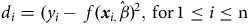 $${d_i} = ({y_i} - \;f{({\boldsymbol x}_{i,}}\hat \beta )^2,\,{\rm for}\,1 \le i \le {\rm n}$$
Using some properties together with the definition of the variance, it is easy to see that
 $$E{\rm{ }}[{d_i}|{{\boldsymbol{x}}_{i,}}\left] {{\rm{ }} = {\rm{ }}E{\rm{ }}} \right[(\;{y_i} - {\rm{ }}f{({{\boldsymbol{x}}_i},\hat \beta )^2}|{x_i},] = Var({y_i}|{{\boldsymbol{x}}_{i,}}).$$
Step 3: The econometric model results serve as the reference for comparing the analyses of the second stage, which is instead based on ML. The ML model is strong in predictive power but needs improvement in explainability. The ML approach portrays the complexity (interaction and nonlinearity) of the relationships among disease infestation, climate change, and production practices. Shrimp income and disease risks require a methodology for completely modeling many covariates that usually coexist in the same environment and are likely to interact. The shrimp production process is risky, but we have little information on the structure of production risk. Hence, the J-P function is preferable to the specifications of other empirical work because it imposes the most miniature set of restrictions on the stochastic technology (Tveterås, Reference Tveterås1997).
ML can handle large datasets with numerous covariates because of its high flexibility (Bertoletti et al., Reference Bertoletti, Berbegal-Mirabent and Agasist2022). To estimate the related risk in the production function model, we use the natural logarithm transformation of the deviance d i obtained from the J-P model as response variables for the various ML models, such as support vector machines (SVMs), random forests (rfModel), and Cubist (cbModel) models. The next section describes or summarizes all these ML algorithms.
Statistical and empirical models
The empirical model is expressed as:
 $${d_i} = {\beta _0} + {\beta _1}{{\rm{x}}_1} + {\beta _2}{{\rm{x}}_2} + \ldots + {\beta _n}\,{{\rm{x}}_n} + {\varepsilon _i}$$
where d
i
is the natural logarithm transformation of the deviance obtained from the J-P and is a function of ${\bf x}_{1}$
……
${\bf x}_{1}$
…… ${\bf x}_{{\rm n},}$
for 1 ≤ i ≤ n. The various independent variables are seen in Appendix I, Table 1, β is a coefficient of regression, and ϵi is the error term. Appendix I, Table 1 shows the anticipated signs for the J-P, income risks, and disease prevalence.
${\bf x}_{{\rm n},}$
for 1 ≤ i ≤ n. The various independent variables are seen in Appendix I, Table 1, β is a coefficient of regression, and ϵi is the error term. Appendix I, Table 1 shows the anticipated signs for the J-P, income risks, and disease prevalence.
Descriptive statistics of selected socioeconomic and biological variables for 534 farmers
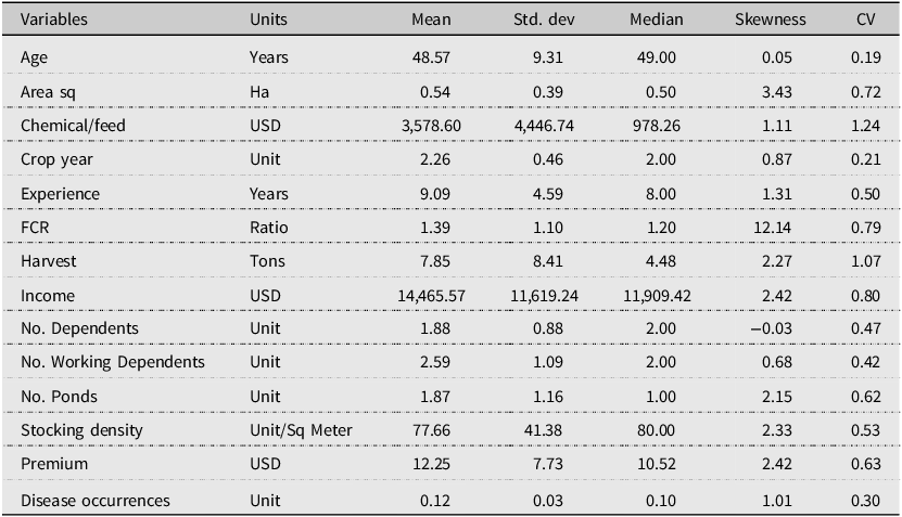
Note: FCR = feed conversion ratio.
Remark 1. We note that our deviance d has a weighted chi-square distribution of 1 degree of freedom for a reasonably small dispersion for each response.
Summary of machine learning methods considered
Linear regression model
A linear model can directly or indirectly be written in the form
 $${y_i} = {\beta _0} + {\beta _1}{x_{i1}} + {\beta _2}{x_{i2}} + \ldots + {\beta _n}{x_{in}} + {\varepsilon _i}$$
where y i represents the numeric response for the ith sample, β 0 represents the estimated intercept, βj represents the estimated coefficient for the jth predictor, x ij represents the value of the jth predictor for the jth sample, and ϵ i is the random error that the model does not explain (Appendix II provides a further description of the ML models).
Hence, the least squares linear regression plane that minimizes the sum-of-squared errors between the observed and predicted values:
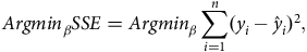 $$\textit{Argmi}n_{\beta }SSE=\textit{Argmi}n_{\beta }\sum _{i=1}^{n}(y_{i}-\hat{y}_{i})^{2},$$
where yi is the outcome and $\hat{{\rm y}}_{{\rm i}}$
is the model prediction.
$\hat{{\rm y}}_{{\rm i}}$
is the model prediction.
Partial dependence plots (PDP)
The determination of predictor importance is a crucial task in any supervised learning problem. Once a subset of “important” features is identified, it is often necessary to assess the relationship between them (or a subset thereof) and the response variable. This can be done in many ways, but for ML, this is accomplished by constructing PDPs. PDPs show the impact of one or two variables on the predictive outcome (Nguyen et al., Reference Nguyen, Nguyen, Nguelifack and Jolly2022a). The PDPs are “partial” since they can only display one or two features at any time (Bracke et al., Reference Bracke, Datta, Jung and Sen2019). The PDP plots enable visualization and analysis of the interaction between the response variable and one or two selected independent variables. From this visual image, the reader can observe the nonlinearities of the relationship between the response and input variable. For instance, using a real-world example, like between stocking density and risk income, the J-P model’s prediction shows that income and disease risks increase. For linear models, the marginal effects (MEs) of the variables of interest are constant over a given range and are described entirely by the values of the estimated parameters. ML offers global approaches as the PDPs are plots that show importance over all the input data ranges, which can be nonlinear, positive, and or negative over a range. In the case of stocking density and income risk, the literature on biological response suggests nonlinearity.
Shrimp farming risks and variable selection
In shrimp farming, the risk is a combination of the likelihood of an adverse event, such as disease outbreaks, and the severity of the associated losses (Choudhary and Madaan, Reference Choudhary and Madaan2016). Shrimp farmers face risks from various sources, including environmental factors, production inputs, and disease prevalence. The relationship between risk and net income is often complex, and traditional economic theory suggests that higher risks are associated with higher potential returns. However, these returns are less likely to be realized (Appendix I, Table 1). Therefore, managing risks in shrimp farming is essential for maximizing profitability while minimizing potential losses.
One of the main risks in shrimp farming is disease. Disease prevalence often increases with factors such as high stocking densities, poor water quality, and intensive farming practices. Shrimp farmers must balance the need to increase production with the risks associated with higher disease prevalence. This balance is further complicated by the fact that many disease risks are influenced by climatic and environmental factors, which are often beyond the control of individual farmers.
Regarding input variables, feed is one of the most important factors influencing shrimp production. While increasing feed levels can boost production, excessive feeding can lead to waste accumulation, reduced oxygen levels, and increased shrimp mortality. Labor, capital, and other production inputs also play a role in determining net income and risk levels. For example, access to credit can help farmers invest in better equipment or sanitation measures, reducing income and disease risks.
Demographic factors such as farmer age and experience influence shrimp farming risks. Older farmers may be more risk-averse and less likely to adopt new technologies or farming practices, which can limit their ability to manage risks effectively. Conversely, more experienced farmers may have better risk mitigation strategies, such as implementing disease prevention measures or adjusting stocking densities.
Managing risks in shrimp farming
Farmers can adopt various risk management strategies to mitigate the risks associated with shrimp farming. These include both preventive and curative measures. Preventive strategies, such as improving water quality, reducing stocking densities, and using disease-resistant shrimp breeds, can help minimize the likelihood of disease outbreaks. Curative measures, such as treating infected ponds, are often less effective, as limited treatments are available for many shrimp diseases.
One important risk management strategy is to invest in sanitation measures, such as installing sludge treatment areas and monitoring water quality more closely. By reducing the buildup of waste and toxins in the shrimp ponds, farmers can lower the risk of disease and improve overall production outcomes. Access to timely information about disease outbreaks is also crucial for managing risks. Farmers who are well-informed about potential disease threats can take proactive steps to protect their shrimp populations, such as reducing stocking densities or adjusting feeding schedules.
Data collection
The data collection process began after obtaining approval from the university’s Internal Review Board. Focus group discussions and meetings with key informants were conducted to gather preliminary insights on farm sizes, farming practices, management strategies, production processes, and marketing approaches in shrimp farming. These discussions helped shape the questionnaire for the subsequent survey.
The sampling process was carried out in four distinct stages. First, two provinces in the Mekong Delta region of Vietnam, Ben Tre and Trà Vinh, were selected for their involvement in pilot insurance programs and their large-scale production of intensive and semi-intensive WLS. Additionally, two other provinces, Khánh Hòa in central Vietnam and Quang Ninh in the northeast, were chosen due to their significant shrimp production levels and vulnerability to climate-related disease risks in shrimp farming (research area seen in Appendix I, Figure 1).
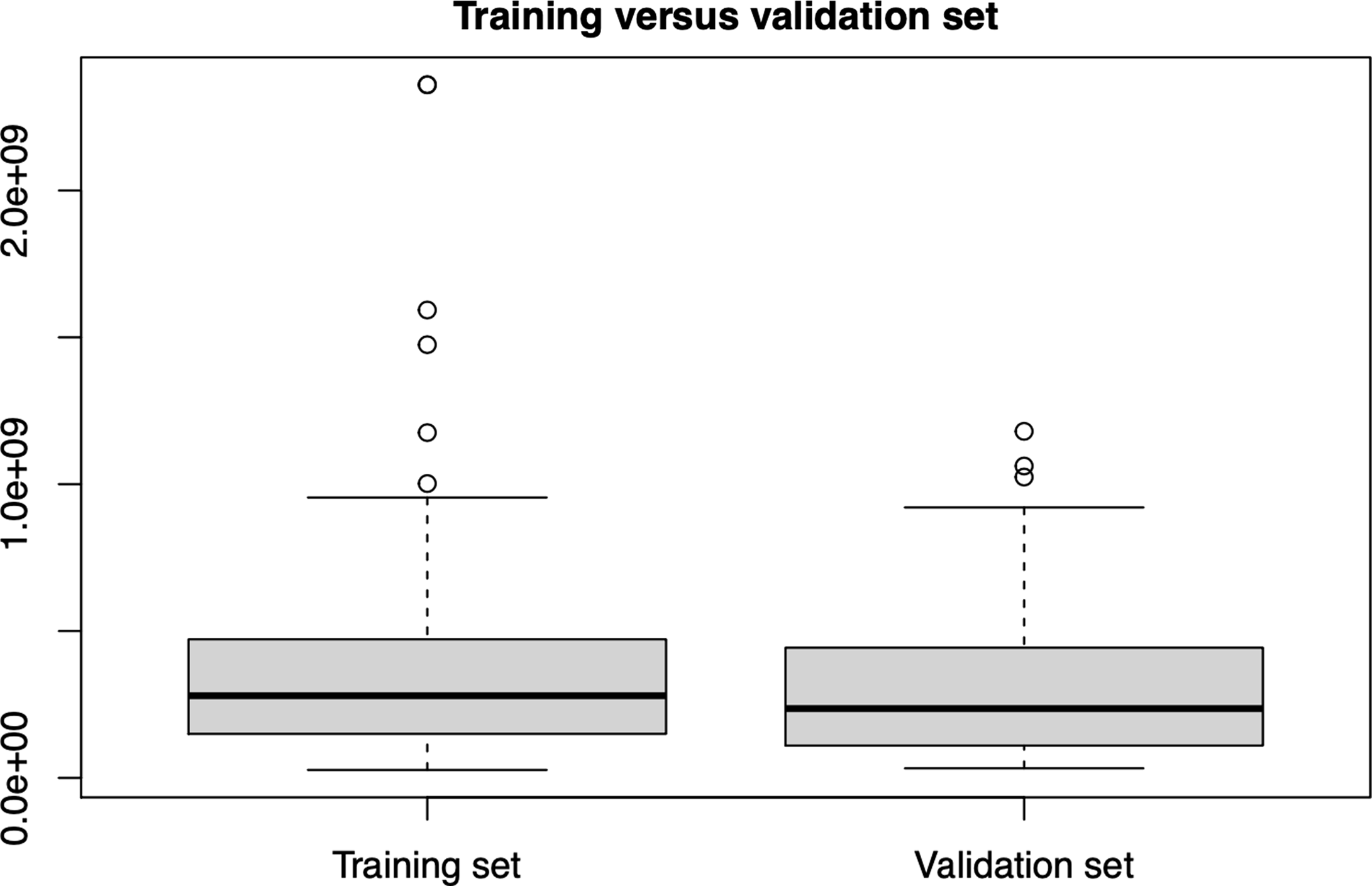
Distribution of the training and validation sets. This figure illustrates the distribution of data points in the training and validation sets, which exhibit similar patterns. The consistent distribution suggests that the model will likely perform well during validation, as both sets encompass the same range of features. This alignment indicates that the validation set represents the training data, which is crucial for assessing the model’s generalization capability.
In the second stage, lists of shrimp farmers were obtained from the provincial agricultural extension offices. These lists provided a base for proportional random sampling, which was implemented in the third stage. The sample included farmers who produced shrimp under intensive and semi-intensive systems, adhering to recommended practices. The sample consisted of 160 farmers from Trà Vinh, 140 from Ben Tre, 125 from Quang Ninh, and 125 from Khánh Hòa, totaling 550 farmers.
Before the main survey, a pre-test of five questionnaires from each province was conducted to assess farmers’ understanding of the survey. The questionnaire covered various topics, including the physical structure of farms, farming systems, farm ownership, management practices, risk management, biosecurity measures, and disaster management strategies. In addition to the socioeconomic and financial aspects of shrimp farming, it explored disease occurrence, natural disasters, and risk management measures.
The survey also addressed farmers’ participation in Vietnam Good Agricultural Practices, Good Agricultural Practices, or Aquaculture Stewardship Council certification programs, as well as their self-improvement efforts. A total of 534 completed surveys were collected from farmers in Trà Vinh (159), Ben Tre (135), Quang Ninh (120), and Khánh Hòa (120), after adjusting for missing data.
Once a randomly selected farmer declined participation, we used a snowball sampling technique, asking the farmer to recommend another with similar farming operations. After inputting missing data, the final descriptive statistical dataset is presented in Table 1 for quantitative variables and Table 2 for qualitative variables, which is further explained in Appendix I, Table 1.
Frequencies and percentages of answers to shrimp risk management questions
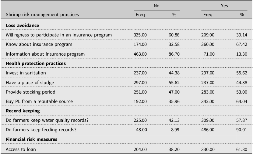
Note: PL= post-larvae.
Data analysis
The data analysis process involved several pre-processing techniques, such as data imputation, transformation, and deletion, to ensure the dataset was suitable for modeling. These methods were crucial for handling missing values and ensuring the analysis was based on a comprehensive and clean dataset. Given the small sample size of 550 farmers, it was important to avoid reducing the sample size further. Missing values, which accounted for 18% of the data, were addressed using the K-nearest neighbor imputation method. This technique, which Troyanskaya et al. (Reference Troyanskaya, Cantor, Sherlock, Brown, Hastie, Tibshirani, Botstein and Altman2001) recommended for high-dimensional data with small sample sizes, estimates missing values by finding the closest samples in the training set and averaging their values. Only quantitative features underwent this imputation process. An analysis with and without the missing variables estimated for the observations was conducted for linear regression and the Rainforest Models. There were noted improvements in the models’ R2 and mean square error (MSE), with the estimated missing data points (Appendix I, Table 2).
The dataset was split into two subsets: 80% for the training set and 20% for the holdout test set. This split allowed for model tuning and evaluation of each predictive model. Given the relatively small sample size, repeated resampling during model training was essential to improve the predictive accuracy of the models. Consequently, a 10-fold cross-validation was performed four times to ensure robust model performance. The splitting technique and its results are depicted in Figure 1, which shows the distribution of the training and validation sets. The selection of the independent variables might create a problem of multicollinearity. However, a test of collinearity using the variance inflation factor (VIF) showed that multicollinearity was not a problem since a VIF value greater than 5 indicates potential multicollinearity issues. None of the variables showed significant concern (VIF<5), suggesting that none could be highly correlated with other predictors (Appendix I, Table 3).
Results of the ordinary linear regression model with a log transformation of the response variable income risks
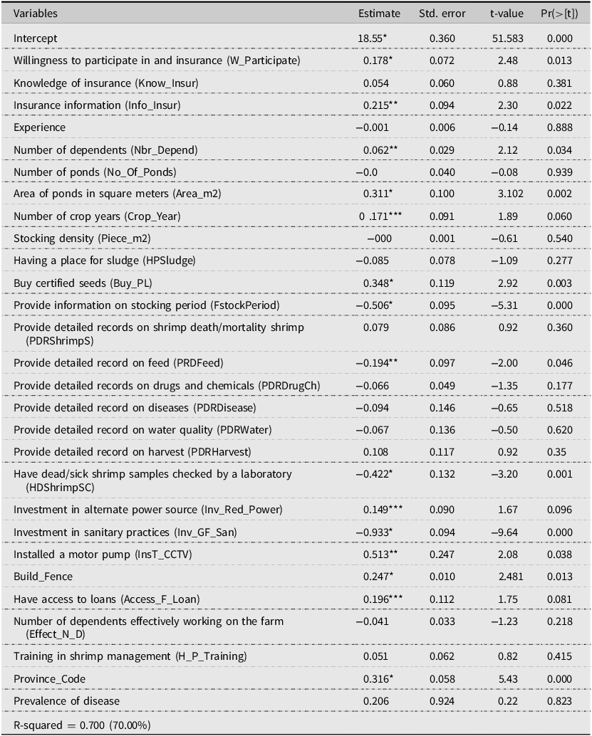
*α=0.01 ** α=0.05 *** α=0.1
Results
The data collected from the survey were thoroughly analyzed, and the findings are presented in this section. Table 1 provides descriptive statistics on the variables used in the analysis. Out of the original 550 surveys, 534 completed questionnaires from farmers in Trà Vinh, Ben Tre, Quang Ninh, and Khánh Hòa provinces were retained after accounting for missing data. The imputation process adjusted the final sample size for analysis. A significant portion of the farmers surveyed (60.9%) expressed unwillingness to adopt risk management tools, such as insurance programs, despite 86.7% of them having some knowledge of insurance options (Table 2). The hesitation may stem from uncertainty about the net benefits of participating in such programs. However, farmers showed risk-reducing behavior in other areas. Approximately 92.95% of respondents invested in alternative power supplies for their farms. Additionally, around 44.3% implemented proper sludge disposal practices, and over 50% purchased post-larvae (PL) from certified distributors (64.04%), followed by stocking periods announced by local authorities (53.0%), and invested in sanitation measures (55.62%).
Farmers also demonstrated strong record-keeping habits, with over 60% maintaining detailed records on stock and stocking practices, feed and feed conversion ratio, water quality parameters, chemical usage, harvest and revenue data, and laboratory samples of diseased shrimp. However, only 27.53% of farmers had registered their farms with government authorities, and 40.7% had obtained some form of farm certification. Furthermore, 61.8% of respondents stated they had access to loans, a vital resource for managing financial risks.
Income risk model results
J-P model results
Income risk is a critical aspect of farm management, and understanding the factors that influence it is essential for developing effective risk management strategies. Table 3 shows the results of the income risk model, based on the J-P regression model using an OLS approach with a log-transformed dependent variable. The model exhibited a solid fit, with 70.0% of the variation in income risk explained by the independent variables.
Several variables were found to be significant predictors of income risk. At the α=0.01 level, key variables included Willingness to Participate in an Insurance Program (W_Participate), Area in Production (Area_m2), Buying PL from certified nurseries (Buy_PL), Fish Stock Period Information (FstockPeriod), Having Sick or Diseased Shrimp Samples Checked by a Laboratory (HDShrimpSC), and the Provincial Code (Province). Additionally, at the α=0.05 level, variables such as Information on insurance (Info_Insur), Providing Detailed Records on Feed Used (PRDFeed), and Installing a Motor Pump (InsT_CCTV) were significant. Finally, the Number of Dependents (Nbr Depend), Crop Year (Crop_Year), Investment in alternate power source (Inv_Red_Power), and Having access to loans (Access_F_Loan) were significant at the α=0.1 level. However, the variables Willingness to participate in an insurance had unexpected signs; insurance information, buying certified seeds, Investment in alternate power source, installing a motor pump, and building fence had unexpected signs that ML must be clarified further.
Modeling disease risk prevalence
J-P model results
The factors affecting disease risk prevalence were analyzed using the J-P regression model, and the results are presented in Table 4. The model demonstrated good explanatory power, with an R2 value of 0.49, indicating that the variation in the independent variables could explain 49 % of the variation in disease risk prevalence.
Ordinary linear regression model results with a log transformation of response variable disease risks
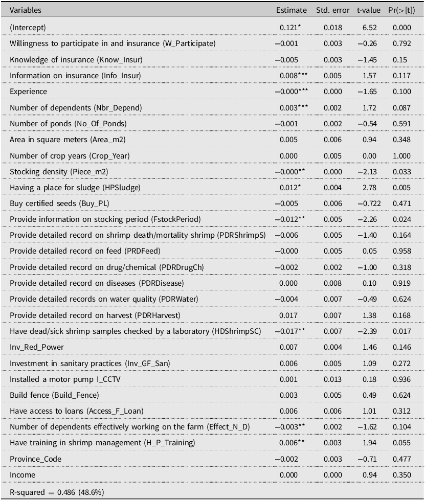
* α=0.01 ** α=0.05 *** α=0.1
The only significant predictor of disease risk prevalence at the α=0.01 level was Having a Place for Sludge Disposal (HPSludge). Additionally, at the α=0.05 level, Stocking Density (Piece_m2), Providing information on stocking period (FstockPeriod), Have dead/sick shrimp samples checked by a laboratory (HDShrimpSC), the Number of Dependents Effectively Working on the Farm (Effect_N_D) and participation in shrimp management training programs (H.P. Training) were significant. At the α=0.1 level, Knowledge of Insurance (Know Insur), the Number of Dependents (Nbr Depend), Experience, and number of dependents (Nbr_Depend) were also significant predictors of disease risk prevalence.
The signs of the variables Having a place for sludge, Information on insurance, and Have training in management were unexpected. Still, the results provide valuable insights into the factors that influence income and disease risks in shrimp farming and highlight the importance of risk management strategies tailored to farmers’ specific needs.
ML model results
One of the main advantages of using ML models is their flexibility in adapting to the structure and complexity of the data. This flexibility allows researchers to select the best combination of models for a specific problem (Storm et al., Reference Storm, Baylis and Heckelei2020). This study explored three ML models: SVM, Random Forest (RF), and a custom-built cbModel model. After running statistical tests, we found that the best-performing models were the RF and cbModel. These models demonstrated low MSE and high coefficient of determination (R 2), indicating their strong predictive capabilities.
A Bonferroni test revealed no significant difference between the RF and cbModel, making both models suitable for examining the relationships between income risks and the covariates. Additionally, RF and SVM emerged as the top models for evaluating relationships between disease prevalence risks and their respective covariates. The next analysis stage aimed to explore the nonlinear effects between income risks and disease prevalence risk variables using ML models.
Covariate analysis of income risks
In this phase, the focus is not on the causality of the effects but rather on ranking the most important predictors for the RF and cbModel. The variables of importance within each model were normalized to sum to one, allowing for an easier comparison of the relative importance of each variable. While the ranking differed somewhat between the RF and cbModel, and the cbModel had only 11 variables of importance, they shared approximately nine of the same important variables.
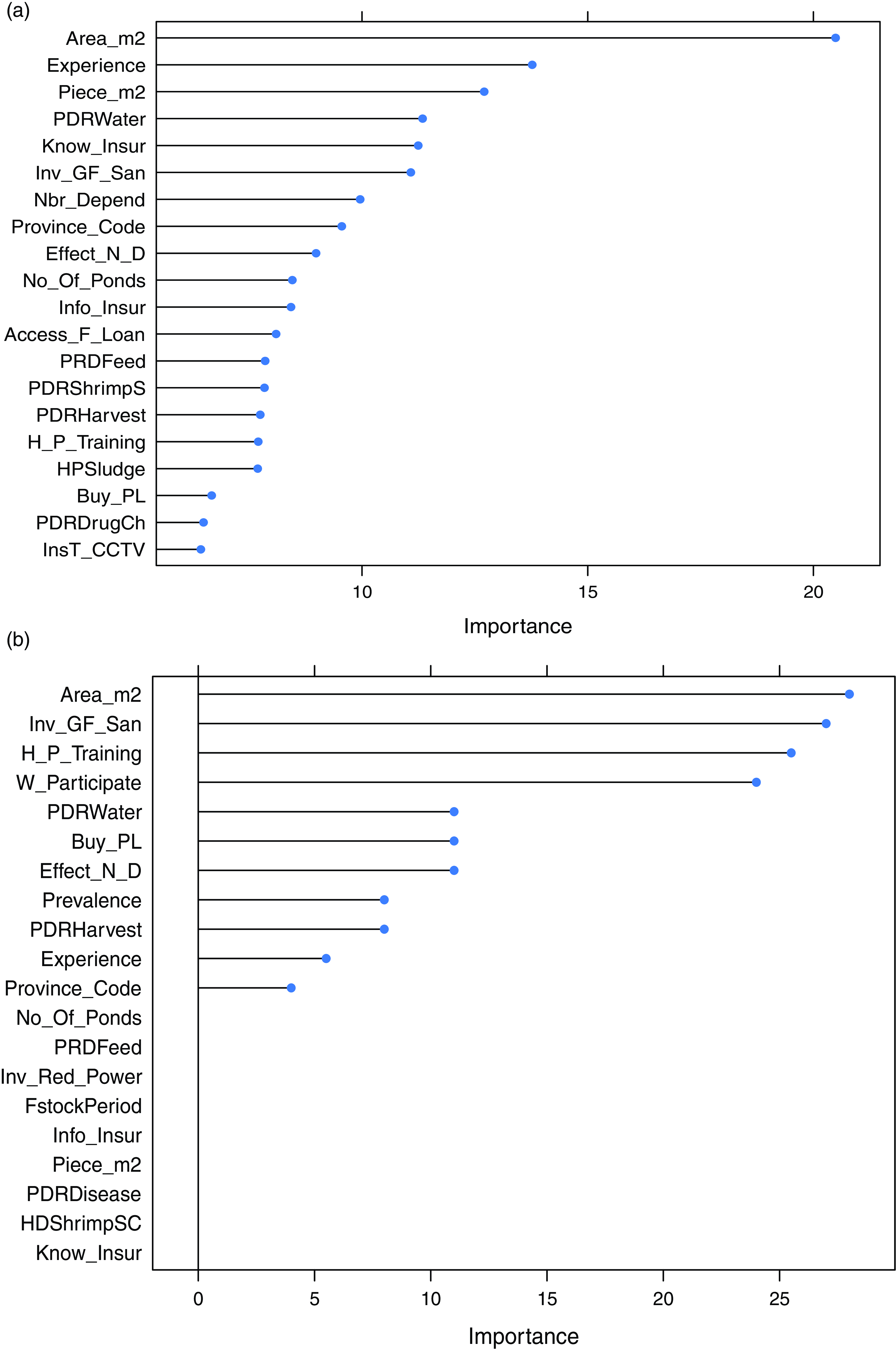
In the RF model, the top-ranking predictor was Area in Production (Area_m2), followed by Experience and stocking density (Piece_m2) (Figure 2a). Other variables like Investment in Sanitary Practices (Inv_GF_San) and Providing Information on Stocking Period (FstockPeriod) appeared lower in the ranking. The cbModel, on the other hand, ranked Area in Production (Area_m2) and Investment in sanitary practices (Inv_GF_San) at the top of the list (Figure 2b). The least of the important variables in cbModel included Have Death/Sick Shrimp Samples Checked by a Laboratory (HDShrimpSC) and Knowledge of insurance (Know Insur).
(a) Variable of importance using the Random Forest (RF) model. This figure displays the importance of each variable in the RF model. Each bar represents the contribution of the corresponding variable to the model’s predictions. Variables with greater importance are more influential in driving the model’s decisions, indicating which factors are most critical for understanding the underlying patterns in the data. (b) Variable importance using Cubist (CB) model. This figure displays the importance of each variable in the CB model.
Covariate analysis of disease risks
Figures 3a and 3b visually represent each covariate’s MEs on disease prevalence risks for the RF and SVM models. Both models help to shed light on how each independent variable influences disease prevalence. For instance, in the RF model, the top three contributors to disease prevalence were Area in Production (Area_m2), Purchase of Certified Seeds (Buy_PL), and Stocking Density (Piece_m2). Conversely, variables like Investment in Alternative Power (Inv_Red_Power), Information about Insurance (Info_Insur), and Willingness to Participate in Insurance (W_Participate) ranked lowest in importance.
Importance of variable using Random Forest (RF) model on the left (a) and support vector machine (SVM) model on the right (b). Here, the risk-related disease prevalence significant variables are the RF and SVM models.
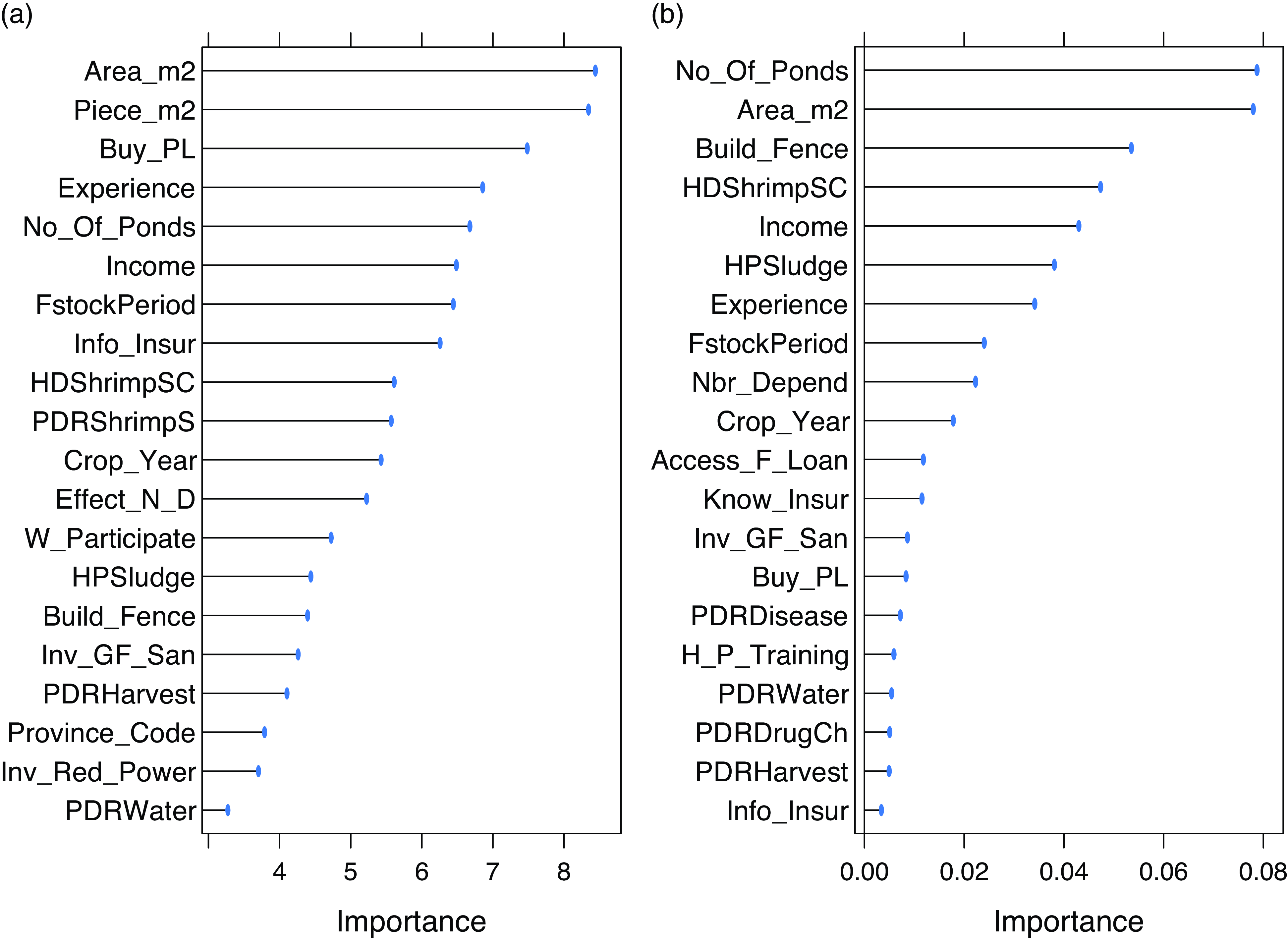
Certified seeds are crucial in disease prevalence since vertical transmission of pathogens like White spot syndrome virus (WSSV) from hatcheries is standard (Hasan et al., Reference Hasan, Haque, Hinchliffe and Uilder2020). Moreover, higher stocking densities increase disease transmission rates, particularly in semi-intensive farms (Hasan et al., Reference Hasan, Haque, Hinchliffe and Uilder2020). The SVM model showed that Area in Production and Number of Ponds (No. of Ponds) were the major contributors to disease risks. At the same time, the Purchase of Certified Seeds and Information about Insurance had minimal influence.
Comparison of J-P and ML models
Income risk models
Table 5 compares the significant variables identified in the J-P models to those found using ML models (RF, cbModel, and SVM). The J-P model had 13 significant variables, whereas the RF model identified 20 significant variables for income risks, of which 8 of 13 (61.5%) were also flagged by the J-P model. The cbModel had 11 important variables, of which 8 (77%) of the variables were aligned with RF covariates, while 4 (30.7%) were like RF covariates. This comparison demonstrates that while the J-P regression model captures the key variables, the ML models may offer a comprehensive view by identifying nonlinear relationships that the J-P model cannot detect.
Significant variables from the J-P models in which the + and - sign indicate that the variables are positively and negatively related, respectively, while for RF, CB, and SVM models, the check mark indicates that the variable tends to be important in the model. The empty cells in the table indicate that the variables are not significant (for J-P) and are not important for other models
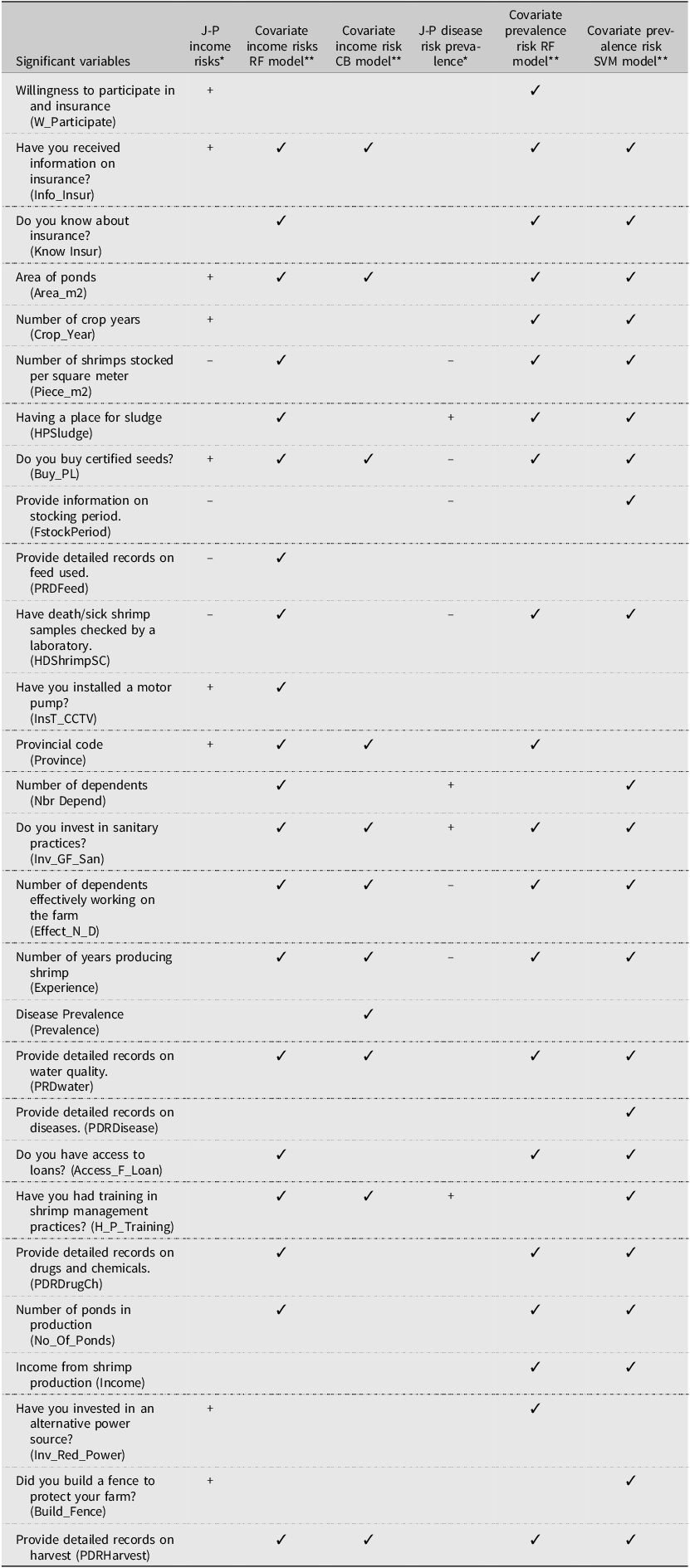
Note: J-P = Just-Pope; RF = Random Forest; CB = Cubist; SVM = support vector machine.
Disease risk models
Similarly, the J-P disease risk model shared seven significant variables with the RF model and eight with the SVM model. Additionally, the RF and SVM models identified 15 variables in common (75%) related to disease prevalence risks (Table 5). This suggests that while the J-P model provides some insight, ML models capture relationships between covariates and disease risks. However, a key advantage of the J-P model is its ability to assign directional signs to variables (indicating whether the effect is positive or negative), a feature that ML models cannot replicate due to their nonlinear nature.
Partial dependency plot visualization and interpretation
Determining the importance of predictors is a critical task in supervised learning. Once a subset of “important” features is identified, assessing their relationships with the response variable becomes necessary. One common technique for achieving this is using partial dependence plots (PDPs). PDPs allow for the visualization of the MEs of each input variable on the model’s predictions (Cook et al., Reference Cook, Gupton, Modig and Palmer2021).
Partial dependency plot of income and selected independent variables
PDPs were used to visualize the effects of independent variables on income risks. For instance, Figure 4a shows that income risks increase rapidly with farmers’ experience before dropping off and then increasing again, albeit at a slower rate. Experienced farmers tend to adopt risk-reducing practices, which could explain this trend (Piamsomboon et al., Reference Piamsomboon, Inchaisri and Wongtavatchai2015; Tendencia et al., Reference Tendencia, Bosma, Usero and Verreth2010).
Partial dependency plot of predicted related income risk versus the top variables using random forest. This figure presents the partial dependency plot illustrating the relationship between predicted income risk and the top influencing variables identified by the Random Forest model. Each curve shows how changes in the top variables affect the predicted income risk while holding other variables constant. This visualization helps to understand the impact of each key variable on the expected outcomes, providing insights into the factors that drive income risk in the dataset. (a) shows the relationship between income risks and experience. (b) shows the relationship between knowledge and income risks. (c) shows the relationship between income risks and a place for sludge. (d) relates income risk and the number of crop years. (e) relates income risk to disease prevalence, and (f) shows the relationship between income risks and pond size.
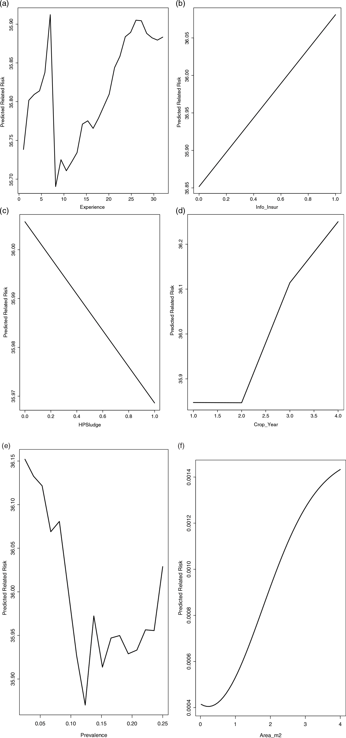
Similarly, insurance knowledge positively influences income risks (Figure 4b). This may be due to higher levels of risk aversion among educated farmers (Outreville, Reference Outreville2015). In another example, Figure 4c shows that income risks decrease when farmers have a designated place for sludge. This practice is encouraged as part of risk management to minimize disease transfer, which can significantly impact farm income through increased costs and yield loss (Nguyen et al., Reference Nguyen, Van, Ngoc, Boonyawiwat, Rukkwamsuk and Yawongsa2021).
The relationship between income risks and crop years shows an initial increase followed by a leveling off (Figure 4d). Over-intensive shrimp production, which can lead to land degradation and increased risks, plays a role in this trend (Bhattacharya, Reference Bhattacharya2009). Similarly, Figure 4e reveals a decline in income risks related to disease prevalence, followed by a slow increase, emphasizing the financial impact of disease outbreaks on shrimp farming (Asche et al., Reference Asche, Anderson, Botta, Kumar, Abrahamsen, Nguyen and Vaderama2021).
Finally, Figure 4f illustrates a sharp increase in income risks with pond size, which eventually flattens out. Larger ponds are often associated with more significant income risks due to the increased difficulty of managing larger production areas (Szuster et al., Reference Szuster, Molle, Flaherty, Srijantr, Szuster, Molle, Flaherty and Srijantr2003).
Partial dependency plot of disease risk prevalence and selected independent variables
The PDPs in Figure 5 demonstrate the nonlinear relationships between risk variables and disease prevalence. For example, Figure 5a shows a negative relationship between the number of dependents and the disease prevalence of up to two dependents, after which the risk increases. Family composition often plays a significant role in farm management practices (Ahmed et al., Reference Ahmed, Allison and Muir2008).
Partial dependency plot of predicted related disease risk versus the top variables using random forest. This figure presents the partial dependency plot illustrating the relationship between predicted disease risk and the top influencing variables identified by the Random Forest model. Each curve shows how changes in the top variables affect the predicted disease risk while holding other variables constant. This visualization helps to understand the impact of each key variable on the expected disease, providing insights into the factors that drive disease risk in the dataset. (a) shows the relationship between disease risk and the number of dependents living in the family home. (b) shows the relationship between disease risk and the number of years of experience. (c) shows the relationship between disease risk and crop years. (d) relates disease risk and stocking density. (e) relates disease risk to having a place for sludge.
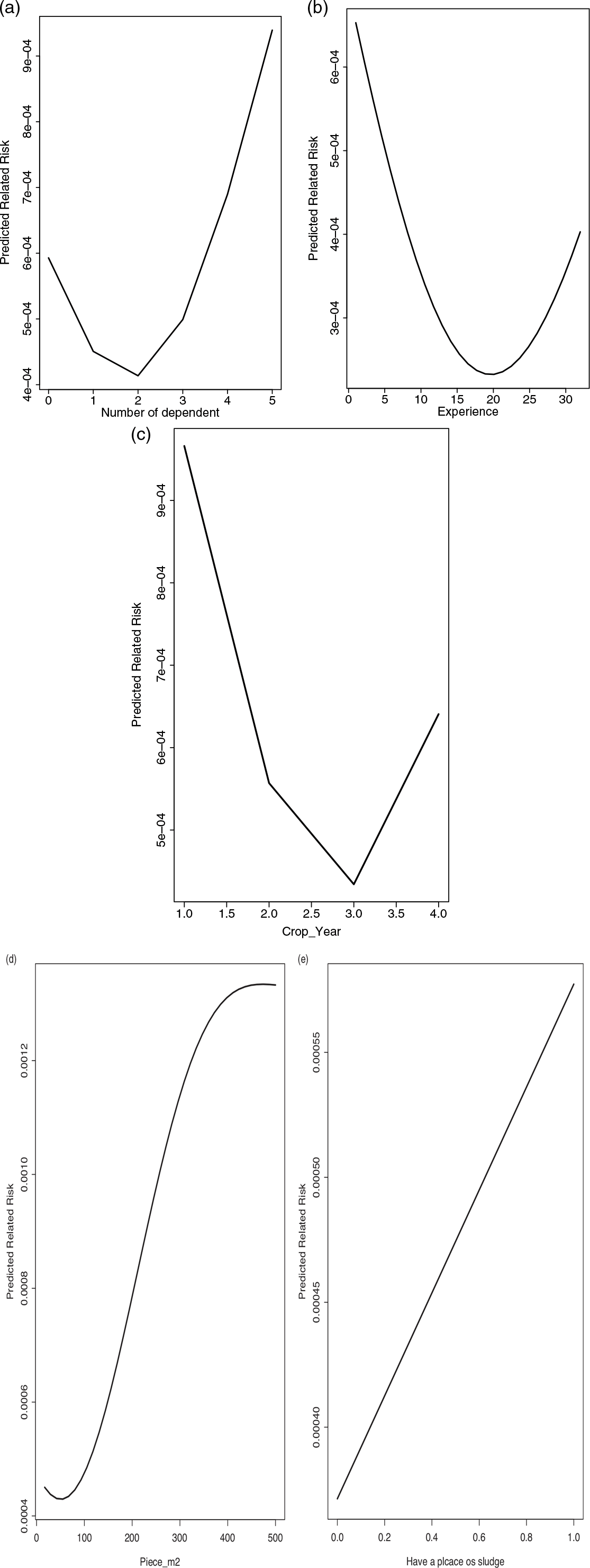
Figure 5b depicts the relationship between years of experience and disease prevalence. It shows that disease risks decline up to 20 years of experience but begin to rise afterward. Younger farmers may adopt more effective risk management strategies than older farmers, making experience a double-edged sword (Phana et al., Reference Phana, Kien, Pabuayon, Dung, An and Dinh2022).
Figure 5c shows a declining relationship between crop year and disease prevalence up to year three, when a sudden increase in disease prevalence is noted. The risk of disease increases with farming intensity (Kautsky et al.,2000). Figure 5d shows a positive relationship between stocking density and disease prevalence. Higher stocking densities are associated with increased disease transmission, particularly in intensive farming systems (Duc et al., Reference Duc, Hoa, Phuong and Bosma2015; Tendencia et al., Reference Tendencia, Bosma and Verreth2011). Similarly, a designated place for sludge removal is negatively related to disease risks (Figure 5e), as effective waste management helps mitigate the spread of infections (Nguyen et al., Reference Nguyen, Nguyen and Jolly2019).
In summary, the PDPs confirm the presence of complex, nonlinear relationships between variables like farm size, stocking density, and experience and the risks associated with income and disease prevalence. These findings highlight the importance of careful farm management to reduce these risks.
Mitigation of independent variables on the dependent variable
Understanding the interaction effects of multiple independent variables on disease risk prevalence is key to comprehensively mitigating these risks. Using PDPs, we can illustrate how changes in combinations of variables influence risk. For example, the interaction between stocking density and pond size highlights how both variables contribute to the increase in prevalence risk (Figure 6a). The prevalence risk remains relatively low when the pond size is smaller than 1.0 ha, and the stocking density is below 100. However, when pond size grows beyond 1.0 ha but remains under 2.75 ha, and stocking density increases between 100 and 300, the prevalence risk accelerates significantly with increasing stocking density. The most concerning scenario occurs when pond size exceeds 2.75 ha and stocking density surpasses 300, rapidly increasing disease prevalence risk. Despite this finding, it is essential to recognize that correlation does not equate to causation. Additional analyses may be needed to confirm whether these variables are causally related to disease risk.
(a) Interaction plot of prevalence-related risk between pond size and stocking density. This figure illustrates the interaction between pond size and stocking density on prevalence-related risk. The plot reveals how varying stocking densities influence risk levels across pond sizes. Understanding this interaction is crucial for effective management practices, as it highlights the conditions under which prevalence risk may increase, enabling stakeholders to make informed decisions regarding optimal stocking strategies. (b) Interaction plot of prevalence-related risk between pond size and income. This figure illustrates the interaction between pond size and income on prevalence-related risk. The plot reveals how variations in income levels influence risk across different pond sizes. This interaction is crucial for understanding the economic factors contributing to prevalence risk, enabling stakeholders to make informed decisions that balance financial outcomes with risk management strategies in aquaculture. (c) Interaction plot of prevalence-related risk between pond size (Area_m2) and experience. This figure illustrates the interaction between pond size (measured in square meters) and the experience level of prevalence-related risk. The plot demonstrates how varying experience levels influence risk across different pond sizes. Understanding this interaction is essential for stakeholders, as it highlights how increased experience can mitigate risks associated with more extensive pond operations, providing insights for better management practices in aquaculture. (d) Interaction plot of prevalence-related risk between stocking density and income. This figure illustrates the interaction between stocking density and income on prevalence-related risk. The plot reveals how changes in stocking density affect risk levels at different income brackets. Understanding this interaction is crucial for aquaculture management, as it highlights how financial factors can influence risk associated with varying stocking practices, enabling stakeholders to optimize their strategies for sustainable and profitable operations.
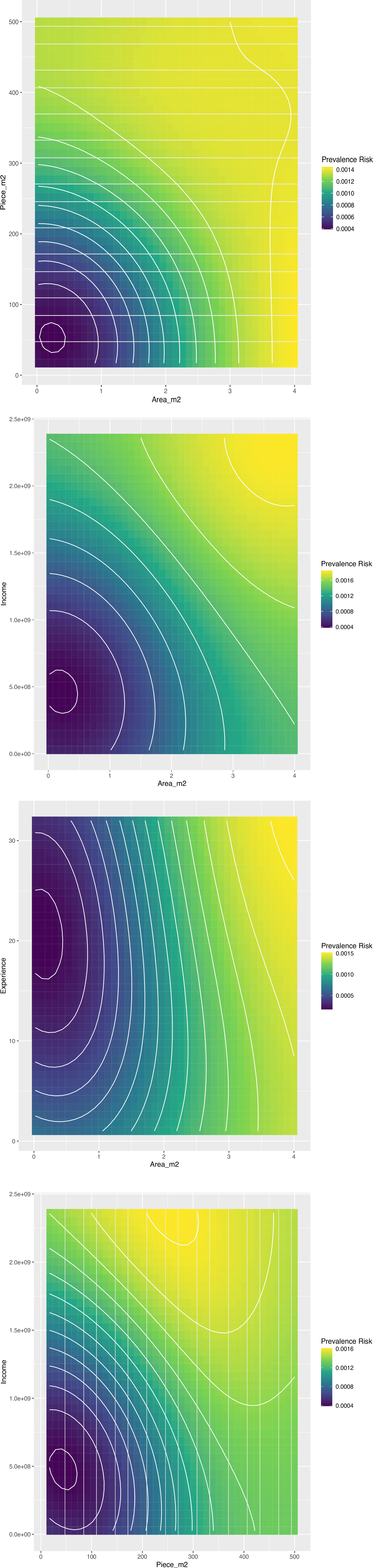
Another critical interaction is between income and pond size (Figure 6b). As both variables increase, prevalence risk similarly rises, with a rapid escalation observed when the pond size exceeds 3.0 ha. For larger pond sizes combined with increased income, disease prevalence risk increases steadily before spiking significantly.
The relationship between farmer experience and pond size reveals important insights (Figure 6c). As pond size increases, so does the prevalence risk, regardless of the farmer’s experience level. Notably, the prevalence risks remain elevated at the highest levels of experience and pond size. However, when experience surpasses 10 years and pond size remains low, the prevalence risk is minimized, highlighting the importance of experience in mitigating risk, especially for smaller operations.
Income and stocking density also strongly correlate with risk prevalence (Figure 6d). When stocking density is between 150 and 275, prevalence risk increases proportionally. However, once stocking density exceeds 275, prevalence risks rise more dramatically. Intriguingly, the prevalence risk decreases somewhat at high stocking densities (above 400). This reduction may be explained by the fact that intensive farming systems with higher inputs often result in higher income but are also associated with more significant risks, particularly shrimp mortality (Bé et al., Reference Bé, Clayton and Brennan2003; Hoa et al., Reference Hoa, Zwart, Phuong, Vlak and Jong2011). As suggested by past research, these intensive systems are vulnerable to fluctuations in harvests, prices, and market conditions, increasing overall risk (Nguyen and Jolly, Reference Nguyen and Jolly2019; Hai et al., Reference Hai, Hao, Abery and Silva2011).
Discussion and conclusion
Shrimp farming is a highly profitable agricultural enterprise that contributes significantly to rural economic development. On average, shrimp farmers in Vietnam earn an estimated net income of USD 18,317.78 per hectare, far surpassing the income generated by other crops. By comparison, Vietnam’s average rural household income between 2012 and 2017 was USD 5,652.17 (Le, Reference Le2020). A farmer with 0.54 hectares dedicated solely to shrimp production equates to an annual household income of around USD 9,991.60, substantially higher than the national average. However, these impressive economic returns come with considerable environmental risks, including the potential for disease outbreaks, which can severely impact income and push farmers toward bankruptcy (Da et al., Reference Da, Phuoc, Duc, Troell and Berg2015; White, Reference White2017). Over 12% of shrimp farmers have experienced disease-related risks in the past year.
The relationship between shrimp disease prevalence and farm income is complex and challenging to decipher due to the variety of farming practices and the limitations of using a single approach to model income and disease prevalence risks. By combining econometric techniques with ML models, this study provides more holistic insights into shrimp disease risk prevalence and mitigation strategies. While the J-P model is traditionally used to evaluate the risk effects of input use in production (Just and Pope, Reference Just and Pope1979), its linear structure limits its ability to capture complex, nonlinear relationships between risks and inputs. In contrast, ML techniques such as RF, cbModel, and SVM excel in detecting these nonlinear interactions and ranking covariates by their importance, offering a more nuanced understanding of how input variables contribute to risk (Kim and Shin, Reference Kim and Shin2021).
In this study, the J-P model identified 13 significant variables influencing income risks, with all but a few having unanticipated signs. The model found 11 significant variables for disease prevalence risks, with four not behaving as anticipated. The J-P income risk model identified more significant variables than the disease prevalence model. However, its limitations in handling complex relationships are apparent compared to the ML models’ results. By incorporating stochastic risk factors, the RF and cbModel showed greater efficiency in selecting important variables for income risks, while RF and SVM performed better in analyzing disease prevalence risks.
While identifying the factors influencing income and disease prevalence risks is critical, it is insufficient to understand how input variables affect these risks fully. The J-P model generates directional signs that show whether a variable positively or negatively impacts the risk response variable. However, ML techniques provide additional insights by mapping complex interactions between variables. This study used PDPs to visualize these nonlinear effects, allowing for a more comprehensive interpretation of the results. For example, the relationship between pond area and income risks shows that risks decline at low pond areas but increase dramatically beyond certain thresholds (Figure 4f). Similarly, the relationship between disease risks and experience illustrates that risks decrease up to 20 years of experience before increasing again (Figure 5b). Stocking density and disease risks also exhibit complex, nonlinear relationships, with disease risks reaching a minimum of around 75 pieces/m2 and rising at an accelerating rate (Figure 5d).
The joint use of the J-P and ML models provides complementary insights. While the J-P model offers clear directional signs, the ML techniques reveal the underlying complexities of variable interactions. For instance, the PDPs reveal nonlinear relationships that are not captured by the J-P model, such as the interaction between stocking density and pond size in determining disease prevalence risks (Figure 6a). By combining these two modeling approaches, researchers can better understand the factors influencing income and disease risks and tailor risk mitigation strategies accordingly.
In conclusion, combining econometric and ML models offers a powerful approach for analyzing complex data in shrimp farming. The J-P model is valuable for generating risk factors, while ML models rank covariates and reveal nonlinear relationships. The two methods are complementary, and their joint usage enables a more robust interpretation of the results. This study highlights the importance of employing multiple analytical techniques to understand better the risks associated with shrimp farming and develop effective strategies for risk mitigation. Additionally, the use of PDPs enhances the visualization of variable interactions, providing actionable insights for both economists and shrimp farmers. Despite some limitations, such as the need for further justification in selecting algorithms, the combined use of J-P and ML models represents a promising direction for future research in the field. In conclusion, ML models like RF and cbModel and tools such as PDPs offer powerful methods for predicting and managing risks in shrimp farming. Farmers can make more informed decisions and adopt strategies that help mitigate risks while maximizing production and profitability by understanding the relationships between input variables and outcomes. As shrimp farming continues to grow in importance globally, these tools will become increasingly valuable for ensuring the long-term sustainability and success of the industry.
Supplementary material
The supplementary material for this article can be found at https://doi.org/10.1017/aae.2025.8.
Data availability statement
The data pertaining to this study are available upon request from Dr Tram Anh Thi Nguyen at anhntk@ntu.edu.vn.
Acknowledgments
The authors would like to thank the ClimeFish Project, supported by the European Union’s Horizon 2020 Research and Innovation Programme under Grant Agreement No. 677039, and the NORHED Project (QZA-0485, SRV-13/0010) for their support in preparing this paper.
Author contribution
All authors participated in the preparation of the paper. However, for conceptualization, Curtis M. Jolly and Brice Nguelifack were mainly responsible; methodology, Curtis M. Jolly, Brice Nguelifack, and Tram Anh T. Nguyen; software, Brice Nguelifack; validation, Brice Nguelifack and Kim Anh T. Nguyen; formal analysis, Brice Nguelifack and Curtis M. Jolly; investigation, Curtis M. Jolly, Tram Anh T. Nguyen and Brice Nguelifack; resources, Tram Anh T. Nguyen and Kim Anh T. Nguyen; data curation, Tram Anh T. Nguyen and Kim Anh T. Nguyen; writing – original draft preparation, Curtis M. Jolly and Brice Nguelifack; writing, Curtis M. Jolly and Brice Nguelifack – review and editing, Curtis M. Jolly and Tram Anh T. Nguyen; visualization, Brice Nguelifack and Kim Anh T. Nguyen; supervision, Kim Anh T. Nguyen; project administration, Kim Anh T. Nguyen and Curtis M. Jolly; funding acquisition, Brice Nguelifack, Tram Anh T. Nguyen, and Curtis M. Jolly. All authors have read and agreed to the published version of the manuscript.
Financial support
This research did not receive a specific grant from any funding agency, commercial, or not-for-profit sector. However, the authors will seek funds from their institution to pay for publication.
Use of AI: AI was not used to write any section of the paper.
Competing interests
All authors declare no competing interests.


 Open access