

1 INTRODUCTION
The stellar populations in a galaxy is a complicated mixture of stellar populations with varying ages and chemical composition. The standard procedure for untangling unresolved stellar populations in galaxies is to take a population model and construct a composite spectral energy distribution (SED) from a library of stellar spectra (Cid Fernandes et al. Reference Cid Fernandes, Schoenell and Gomes2009; Franzetti et al. Reference Franzetti, Scodeggio, Garilli, Fumana and Paioro2008; Li & Han Reference Li and Han2008; Schulz et al. Reference Schulz, Fritze-v. Alvensleben, Möller and Fricke2002) which is then convolved by the filter set of interest and compared to the photometry of galaxies. While the evolution of stars is a fairly well understood field, application of stellar evolution models to galaxies is complicated by the shear weight of the number of different types of stars involved (limited by the depth of the stellar spectral library), the difficulty of comparison observations and complicated ISM physics.
The starting point for a stellar synthesis program is the construction of the simplest stellar population, one where all the stars are a single age and chemical composition (e.g., a globular cluster). As all the details of stellar evolution are known, then they only variable is the initial mass function (IMF) which assigns the number of stars per mass bin. Each mass bin follows a specific evolutionary track resulting in the color-magnitude diagram as a function of time which is summed to produce an SED (or a set of colors and indices). These stellar population models are called simple stellar populations (SSP’s, see Schiavon Reference Schiavon2007 for a review) in order to recognise their limited initial parameters, not to minimise the computational difficulty of the modeling.
Galaxies, however, are not SSP’s simply from the fact that all the stars could not have been produced in a single, simultaneous burst of star formation. Star formation must have been temporally extended, as seen in the metallicity gradients found in ellipticals and spirals. Spatially extended information about a galaxy provides a great deal of information on the changes in age and metallicity internal to the system but, unless the resolution discerns the actual stars, each resolution element in the galaxy (i.e., each pixel) is still a composite form of the stellar light. Thus, the unraveling of the underlying stellar population from its composite spectrum may be an intractable problem even on small spatial scales.
A great deal of the focus in producing SSP’s was on globular cluster and early-type galaxies due to their assumed simpler histories of star formation. Star clusters were a prime target, for the integrated spectrum could be modeled then checked by direct comparison to the cluster’s color-magnitude diagram (CMD, Schiavon Reference Schiavon2007). Ellipticals were the next focus as early color and spectroscopic work indicated their stellar populations were very similar to globular clusters (Burstein et al. Reference Burstein, Faber, Gaskell and Krumm1984, Schombert & Rakos Reference Schombert and Rakos2009) and they lack any signs of ongoing star formation (i.e., Hα emission). Success in modeling ellipticals is measured by the enormous volume of work using colors and spectral indices to deduce ages and metallicities (Trager et al. Reference Trager, Faber, Worthey and González2000; Kuntschner et al. Reference Kuntschner, Lucey, Smith, Hudson and Davies2001; Poggianti et al. Reference Poggianti, Bridges and Carter2001; Gallazzi et al. Reference Gallazzi, Charlot, Brinchmann, White and Tremonti2005; Thomas et al. Reference Thomas, Maraston, Bender and Mendes de Oliveira2005; Sánchez-Blázquez et al. 2006; Rakos, Schombert, & Odell Reference Rakos, Schombert and Odell2008). While a large number of issues still need to be resolved, such as the details of short-lived stellar phases (blue horizontal branch and TP-AGB stars) and their impact on present colors and the evolution of color with redshift, progress in the details of stellar population synthesis has been substantial (Conroy, Gunn, & White Reference Conroy, Gunn and White2009).
Spirals are much more difficult objects to model as their total stellar populations include an elliptical-like bulge and a star-forming disk (to varying degrees along the Hubble sequence). This leads to a problem in interpreting colors and spectral features due to the age-metallicity degeneracy (Worthey, Trager, & Faber Reference Worthey, Trager and Faber1995) and the complications due to a highly variable (spatially and in density) ISM (Kennicutt et al. Reference Kennicutt, Hao and Calzetti2009). Irregulars were actually better candidates to study stellar populations due to their closeness to the Milky Way and more visible star formation regions (less optical depth), as well as typically lower stellar masses and metallicities which serves to compress the age-metallicity degeneracy effect (Hunter & Elmegreen Reference Hunter and Elmegreen2004).
Successful modeling of spirals and irregulars has reproduced many of their large scale characteristics, such as the color-magnitude and the Tully-Fisher relation (Boissier & Prantzos Reference Boissier and Prantzos2000, Bell & Bower Reference Bell and Bower2000). These models have also been successful at understanding the relationship between gas density and the star formation rate (SFR), used to develop various star formation laws (Kennicutt & Evans Reference Kennicutt and Evans2012). Adding a chemical evolution model allowed for predictions for the mass-to-light ratios (M/L) and the various color relationships for spirals (Bell & de Jong Reference Bell and de Jong2000). Almost all of the bright, high surface brightness spirals are well fit with models of declining SFR’s, matching the loss of their gas supply with time (Boissier & Prantzos Reference Boissier and Prantzos2000).
Low surface brightness (LSB) galaxies are, in general, not particularly small or low in mass (see Schombert, Maciel, & McGaugh Reference Schombert, Maciel and McGaugh2011). Their only defining characteristic are central surface brightnesses below 23 B mag arcsecs− 2 (the typical spiral has a central surface brightness of 21 B mag arcsecs− 2). A dilemma is posed by LSB galaxies, for their gas fractions are high, their stellar densities are low, their optical colors are blue and their ratio of stellar mass to mean SFR implies a timescale of star formation of a Hubble time (McGaugh & de Blok Reference McGaugh and de Blok1997). The combination of these factors indicates a star formation history that has a much lower mean SFR than most spirals and irregulars plus a history that must be nearly constant SFR (or perhaps evenly spaced bursts), since the time of galaxy formation in order to produce enough stellar mass, yet have present day optical colors that are extremely blue.
While appearing to represent a challenge to star formation models, LSB galaxies may also provide a clearer window into the star formation history of gas-rich galaxies for several reasons. One, they contain much less dust than normal spirals or irregulars (O’Neil & Schinnerer Reference O’Neil and Schinnerer2003). While they are rich in neutral hydrogen, their low stellar surface densities also reflect into low gas cross sections (McGaugh & de Blok Reference McGaugh and de Blok1997), so the effects of the ISM (both dust and gas) on colors are minimal. Second, all indications are that LSB galaxies have very low mean metallicities (McGaugh Reference McGaugh1994). This reduces the range of population models that must be integrated to produce a total spectrum or color and reduces the complications from the different tracks for metal-rich versus metal-poor stars. Third, since the ratio of SFR to stellar mass in LSB is close to unity for a Hubble time then the mean SFR has been nearly constant for LSB galaxies, as a class, over their evolutionary history (Schombert, McGaugh, & Maciel Reference Schombert, McGaugh and Maciel2013, Schombert & McGaugh 2014) which greatly simplifies the modeling. The duration and strength of burst activity can be constrained by examining the scatter in the Hα luminosity versus galaxy mass relation. All the above dramatically reduces the possible model histories down to a set of quasi-static constant SFR scenarios.
The goal of this paper is to outline a series of models to explain the colors of LSB galaxies, using the above constraints on the properties of LSB galaxies that enhance the reliability of population synthesis. Even with the scenario of constant star formation, there still a series of unknowns that must be explored in the models to reproduce the full range of possible color histories. Our models are also extended to wavelengths within the Spitzer telescope imaging range, providing longer wavelength leverage which is critical to separate the influence of TP-AGB stars, metallicity effects and explore a realm where M/L estimates are more stable (Schombert & McGaugh 2014).
2 MODEL PARAMETERS
2.1 Single age composite SSP’s (multi-metallicity models)
The obvious next step beyond a SSP, a population of single age and single metallicity, is a single age composite SSP which includes a range of metallicities that follow a particular enrichment scenario (Pagel Reference Pagel and Pagel1997). Of course, physically, it is impossible to generate enriched stars without a progression of stellar birth and death, then recycling enriched material back to the ISM. This clearly takes a finite amount of time but, fortunately, the recycling timescales are much shorter than noticeable changes in a stellar population due to age (Matteucci Reference Matteucci2007). Enrichment can be treated as instantaneous and the stars can be assumed to arise from an enriched gas with a range of gas metallicities that reflect the metallicity distribution function (MDF) of the stars.
With a proper MDF, a composite stellar population is constructed by extracting from the stellar library stars of a single age and varying metallicities as given by the MDF bins. The resulting spectra are summed and weighted by number to produce integrated colors and indices. The mean metallicity is calculated either as a luminosity weighted value, or a averaged value (i.e. by number). The remaining problem is to determine a MDF that fits the stellar populations in a star-forming galaxy.
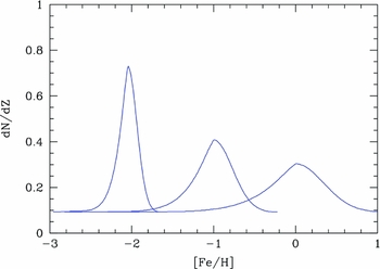
For the current suite of models, we have followed the MDF prescription outlined in Schombert & Rakos (Reference Schombert and Rakos2009) which has the advantage of matching the chemical evolution of Milky Way stars and correctly reproducing elliptical colors. The MDF model adopted in Schombert & Rakos (Reference Schombert and Rakos2009, called the ‘push’ model) is designed to resolve the G-dwarf problem (Gibson & Matteucci Reference Gibson and Matteucci1997, an underestimation of low metallicity stars in closed box models) and incorporates a mixing infall scenario (Kodama & Arimoto Reference Kodama and Arimoto1997, linking the accretion rate to the star formation rate). The resulting MDF (see Figure 4, Schombert & Rakos Reference Schombert and Rakos2009) provides a simple analytic function that can be adjusted for its peak [Fe/H] to reproduce any mean [Fe/H] for a stellar population.
Our ‘push’ model MDF is shown in Figure 1 for three different peak [Fe/H]’s and its general shape follows MDF’s given by theoretical chemical evolution simulations, nearby star counts and HST studies on the tip of the red giant branch (RGB) in nearby ellipticals (Harris & Harris Reference Harris and Harris2000). Nearby galaxies display a lower metallicity peak with increasing radius from the galaxy center (i.e., metallicity gradients). This results in a narrower MDF with lower peak metallicities, but maintains the same general shape.
Three ‘push’ MDF’s are shown for peak [Fe/H] of − 2, − 1 and solar, all having a long tail to low metallicities and a steeper high metallicity side. The effect of depressing the decreasing low metallicity stars (the push to resolve the G-dwarf problem) is evident by the shallower slope on the low metallicity side. Each population is normalised to the same total number, which results in a wider spread in [Fe/H] with increasing peak [Fe/H]. For the low metallicities, the small width means these models are identical to a gaussian or any simple infall model.
The success, and usefulness, of this model is tested by the accuracy that the composite SSP’s colors and indices match globular cluster and elliptical colors over a range of galaxy masses (i.e., total metallicities, Schombert & Rakos Reference Schombert and Rakos2009 b). And, while successful with single burst populations that dominate elliptical stellar populations, there are elements to the ‘push’ model that make it as useful for constant star formation scenarios. For example, the ‘push’ model matches the shape of inhomogeneous enrichment models (Malinie et al. Reference Malinie, Hartmann, Clayton and Mathews1993, Oey Reference Oey2000) where star formation occurs in discrete patches throughout a galaxy and is only allowed to mix between star formation episodes. This increases the amount of mixing and results in fewer metal-poor stars. In fact, our model at solar metallicities is identical to Prantzos (Reference Prantzos2009) infall model with a timescale of 7 Gyrs.
The use of a realistic metallicity spread has an increasing effect on a stellar populations colors with increasing mean metallicity. For a 12 Gyr population with a mean metallicity of < Fe/H > = − 2, the change in optical and near-IR colors is effectively zero as the spread in metallicity is very small. By a mean metallicity value of < Fe/H > = − 1, the change in B − V and V − K is − 0.01. For a solar metallicity population, the difference is − 0.05 in B − V and − 0.02 in V − K (Schombert & Rakos Reference Schombert and Rakos2009). For a younger population, this difference is the same in the optical (age dominates over metallicity) but increases in the near-IR to Δ(V − K) = −0.09 for a solar metallicity population. The effect, overall, is to make all the colors slightly bluer due to the inclusion of a metal-poor component at each epoch, an expected result.
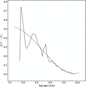
The effect of using composite metallicity models on galaxy colors varies with wavelength. For both near-UV and optical colors, a spread in [Fe/H] results in slightly bluer colors. But, for optical colors, the separation in color between SSP’s and composite models increases with increasing stellar population age. The bottom panel in Figure 2 displays the run of B − V for a solar metallicity population as a function of age. For ages less than 1 Gyr, the differences are minor. By 10 Gyrs, the different between the models is 0.05 mags. While this is small in an absolute sense, it is noticeable in studies of the color-magnitude diagram in ellipticals (Rakos & Schombert 2009).
The effect on B − V and V − K between a single metallicity population (SSP) and a composite population (using our ‘push’ MDF) as a function of age. A peak solar metallicity model is displayed and the differences in colors from adding a distribution of metallicities is particularly noticeable at young ages with the combined effects of young age and a contribution from metal-poor stars drives the RGB to higher temperatures and bluer V − K colors. The difference in V − K fades with time, but the metal-poor stars begin to show differences in optical colors (B − V) as the turnoff point reddens after 1 Gyr. The crossover in V − K color at 10 Gyrs is due to the shape of the MDF having more stars above solar [Fe/H] than below.

The color differences between the composite metallicity models and SSP’s are more direct for near-IR colors. The top panel in Figure 2 displays the run of V − K for the range of ages from 0.1 to 12 Gyrs. As RGB stars dominate the near-IR colors in galaxies, and the temperature of RGB branch is strongly dependent on [Fe/H], strong color differences are found at young ages (0.8 at 0.1 Gyrs) decreasing to zero at 10 Gyrs. The composite models become redder than the SSP’s after 10 Gyrs due to the fact that a spread of [Fe/H] is involved in the composite models which finds the metal-rich stars being brighter than the metal-poor stars for old stellar populations.
The only remaining variable to our MDF simulations is the effect of infalling gas. LSB galaxies are particular gas-rich and, while it is assumed that the low SFR in LSB galaxies is due to low gas densities, the total gas mass of these systems is high. This leads to the increased probability that a significant fraction of the gas supply for star formation is from primordial infalling gas. Mixing models account for some primordial gas in their simulations, but LSB galaxies may have a higher percentage of metal-poor gas than other spirals or irregulars. Our only argument against increasing the metal-poor side of our baseline MDF is that LSB galaxies do not deviate from the color-magnitude diagram from other star-forming galaxies (Schombert & McGaugh 2014). The color-magnitude relation is driven by a mixture of star formation, age and metallicity effects (Tojeiro et al. Reference Tojeiro, Masters and Richards2013) and the colors of LSB galaxies place them at bluer colors than normal spirals in line with their lower metallicities. There is no indication that their metallicities are extremely low, so we have not altered our baseline MDF to allow for a much larger population of metal-poor stars than already accounted for by inhomogeneous mixing scenarios. We also note that due to the lack of detection of dust in any LSB galaxies, either due to low metallicities or simple low stellar densities, we have ignored any internal extinction corrections to our model colors.
2.2 Chemical enrichment model
For star forming galaxies, such as spirals and irregulars, the MDF will continue to evolve as long as star formation continues. The MDF evolution is such that the peak metallicity increases with time plus the rate of evolution is proportional to the rate of star formation. To characterise a changing mean metallicity, the peak [Fe/H] of our ‘push’ model is simply shifted to higher metallicities while maintaining its shape and tying the lowest metallicity end to a zero metallicity gas (effectively [Fe/H] = −2.5, see Figure 1). Each curve is parameterised by the peak [Fe/H], but the mean metallicity (< Fe/H >) and the luminosity weighted [Fe/H] value vary in a linear fashion (see Schombert & Rakos Reference Schombert and Rakos2009).
In order to develop a realistic chemical enrichment scenario, a simple model of chemical evolution is required constrained by actual age-metallicity relations in nearby galaxies. Numerous age-metallicity models have been proposed (Sellwood & Binney Reference Sellwood and Binney2002, Prantzos Reference Prantzos2009) all having the similar initial conditions of a [Fe/H] = −1.5 enriched gas then leveling off after 5 Gyrs (the final [Fe/H] dependent on the mass of the galaxy). However, most models fail to match the run of [Fe/H] with age in our own Galaxy (e.g., Nordstrom et al. Reference Nordström, Stonkutė, Tautvaišienė and Zenovienė2012) where extremely metal-poor stars are rare and the models over-predict their numbers compared to observations.
The difference between models and observations has been attributed to two effects; 1) the large statistical uncertainties in the data, particular for the metal-poor end of the data samples and 2) the impact of radial mixing on the observed Galaxy sample (Prantzos Reference Prantzos2009). The initial metal building phase is critically important to our models since most LSB galaxies appear to have total metallicities much less than normal spirals (McGaugh Reference McGaugh1994). Thus, we need SF models where the final [Fe/H] is in the range of − 1.5 to solar and such that the oldest stellar populations with the lowest metallicities can be included in the synthesis calculations.
To this end, we have adopted the Prantzos enrichment model which rapidly increases the mean [Fe/H] for the first 2 Gyrs (80% yield), then an additional 15% over the next 5 Gyrs and effectively constant for the last 5 Gyrs (assuming a 12 Gyr old galaxy, see Figure 3). The parameterisation for this scenario will be the final generation metallicity ranging from [Fe/H]= − 1.5 to 0.2. To maintain the same shape, we adjust the shape of the age-metallicity relation so that same percentages in each metallicity bin are the same from model to model. The [Fe/H] value at a particular age is taken to be the peak [Fe/H] for the ‘push’ MDF, thus, even in the final generations of stars, some metal-poor component is produced to represent the infall of low metallicity gas into the galaxy. Using a MDF in combination with an enrichment model will result in averaged [Fe/H] that are consistently below the model value (due to the sum of previous metal-poor populations, see Figure 3).
The chemical enrichment scenario taken from Prantzos (Reference Prantzos2009) shown as the blue line. Fixed at [Fe/H] = −1.5 at 12 Gyrs (model start time) and rising to solar at the present day. The green line displays the instantaneous [Fe/H] as a function of age. Since the ‘push’ model is asymmetric, such that there are more higher than peak metallicity stars than below the peak, the instantaneous [Fe/H] is higher that the peak value at all times. The red line displays the running average metallicity (< Fe/H >), displaying the integrated metallicity of all the past stars at each generation. While the Prantzos model is used to set the normalization of [Fe/H] with time, the actual values vary due to the asymmetric shape of the MDF. The final averaged value is used for the analysis diagrams in Section 4.

The effects on galaxy colors of using a multi-metallicity with a chemical enrichment scheme are fairly significant. Compared to a constant SF scenario with an non-evolving solar metallicity population, a chemical enrichment model produces little change in B − V colors, they are bluer by 0.05 mags. However, the difference in the near-IR is substantial with Δ(V − K) of 0.15 with a simple chemical evolution scenario due to the higher sensitive of RGB stars to metallicity. The inclusion of a metal-poor component to the composite population has the strongest effect on the width and position of the composite RGB.
2.3 Initial mass function
The distribution of stellar masses is known as the stellar initial mass function (IMF), i.e. the percentage of stars within specific bins of mass assumed for the stellar population at the onset of star formation. While the onset of thermonuclear fusion may vary by mass within a molecular cloud, the timescale from protostar formation to the main sequence is shorter than the timesteps assumed by our model (10 Myrs). Thus, each stellar population segment is assumed to produce a range of masses already on the main sequence at time zero (i.e., no T-Tauri phase is used in the simulation).
Observations on the shape of the IMF in other galaxies are very limited (Kroupa Reference Kroupa2001) and mostly revolve around indirect measurements, e.g., the effect on galaxy colors due to changes in a model IMF (van Dokkum Reference van Dokkum2008). For simulations of galaxy colors, changes in the upper end of the IMF dominate integrated colors due to the high luminosities of high mass stars. As a stellar population evolves, the upper end of the main sequence feeds into the RGB luminosity to effect near-IR colors. Changes in the IMF below 1M ⊙ have a negligible effect on colors, however, the small changes in the numbers on the lower end of the IMF can have a significant effect on calculated M/L’s for the population (see Section 4.3).
For LSB galaxies, we have a mild constraint on the upper end of the IMF from comparison of star cluster luminosities to Hα emission (see Figure 13 of Schombert et al. Reference Schombert, McGaugh and Maciel2013). To match the upper envelope of the cluster mass to Hα luminosity required a power-law index of − 2.6, compared to the value of − 2.5 from the Kroupa et al. (Reference Kroupa, Weidner and Pflamm-Altenburg2013) formulation. A slightly different slope on the upper end of the IMF has a small effect on the B − V colors (bluer by 0.01), but no effect on colors redward of V. Most of uncertainly that derives from variation in the IMF occurs in colors for populations younger than 3 Gyrs, which make up less than 20% of the final stellar mass. Color effects were concentrated in filters blueward of V, although calculations of M/L are sensitive to the IMF even out to 3.6 mμ (McGaugh & Schombert 2014).
As noted by Conroy et al. (Reference Conroy, Gunn and White2009), a discontinuous slope IMF, such as proposed by Kroupa (Reference Kroupa2001), has the unfortunate effect of introducing irregular jumps in luminosity and color at the timescales where the IMF slope changes. However, the IMF proposed by Chabrier (Reference Chabrier2003) is very similar to the Kroupa IMF, at least for masses less than 10 M ⊙. Thus, we have adopted the Chabrier formulation for our model IMF, with a slightly steeper slope for stars greater than 10M ⊙ (− 2.6).
2.4 α/Fe corrections
The colors of stellar populations is determined by the distribution of stars, given by stellar isochrones, in the HR diagram. Decreases in metallicity drive both the turnoff point and the position of the RGB to hotter temperatures, i.e. bluer colors, due to changes in line blanketing and opacity. While Fe is the main contributor of electrons to produce color changes, all atoms heavier than He can contribute electrons. It is typically assumed that all the elements track Fe abundance, but it is possible to have overabundances of various light (so-called α elements) under certain conditions.
The elements lighter than Fe (the so-called α elements) are primarily produced in massive stars (Type II SN), while a substantial contribution to Fe comes from Type Ia SN. Since SNII are short-lived (τ < 10 Myrs) and SNIa detonate only after a Gyr (the mean time for the white dwarf to form), the ratio of α/Fe measures the formation timescales. At early epochs, the ratio of α/Fe is determined by Type II supernovae (SNII) and after a Gyr, the α/Fe ratio decreases due to the products from SNIa explosions (cf. McWilliam Reference McWilliam1997, and references therein).
For example, in elliptical galaxies the ratio of α/Fe is a factor of four higher than metal-rich stars in the Milky Way due to the short timescales of initial burst star formation (Thomas, Maraston, & Korn Reference Thomas, Maraston and Korn2004). As star formation is extended in spirals and irregulars, those galaxy types have lower α/Fe ratios as more recent star formation is enriched by SNIa Fe (Matteucci Reference Matteucci2007). For a constant star formation scenario, we can model the ratio of α/Fe as a function of [Fe/H] following data from the Milky Way (Milone, Sansom, & Sanchez-Blazquez Reference Milone, Sansom and Sánchez-Blázquez2010) with [Fe/H] serving as a proxy for age. In their data, elliptical-like α/Fe ratios are found up to [Fe/H] = −1.0, then drops quickly to a solar value at solar metallicities. We will apply the same behavior to our simulations.
The effect of the α/Fe ratio on colors was outlined in Cassisi et al. (Reference Cassisi, Salaris, Castelli and Pietrinferni2004). With respect to colors, B − V decreases (bluer) with increasing α/Fe, for example a metal-poor population ([Fe/H]= − 1.3) had a blue shift of − 0.03 for an increase in α/Fe by a factor of four. A solar metallicity population shifted by − 0.07 blueward for the same change in α/Fe. Similar shifts are expected in V − K with Δ(V − K) ranging from − 0.06 for metal-poor populations to − 0.09 at solar metallicity.
To incorporate these corrections into our models, we assume that α/Fe decreases, in a linear fashion (as Fe increases from SN events), from an initial value of 0.4 to a solar value (0.0) over one Gyr of time starting two Gyrs after initial star formation. Thus, only the first three Gyrs of star formation have differing α/Fe values from solar, these populations already have the low metallicities at the end of the simulation, which minimises the effect. For example, changes of Δ(B − V) = −0.02 and Δ(V − K) = −0.06 were calculated in a solar metallicity stellar population at the end of the simulation.
2.5 BHB treatment
Horizontal branch stars are old, low mass (M < 1M ⊙) stars which have entered the helium core burning phase of their lives. They are bright (MV = −5), of nearly constant luminosity and range in color from red to blue (RHB and BHB stars). BHB stars are of interest to galaxy population models for they have similar characteristics to young stars in color parameter space, although they are not a signature of recent star formation.
The effect BHB stars on population models is limited in time and metallicity. BHB stars are primarily found in metal-poor clusters ([Fe/H] < −1.4) and are not found in any population younger than 5 Gyrs. Very few BHB stars are found in the solar neighborhood (Jimenez et al. Reference Jimenez, Padoan, Matteucci and Heavens1998), presumingly a combination of young age and high metallicity, so their contribution in field populations is unclear. At the start of our constant star formation scenario, the simulation finds 58% of the stellar population has the metallicity and age appropriate for a BHB phase. Following the prescription of Conroy et al. (Reference Conroy, Gunn and White2009), this corresponds to a fBHB = 0.6 which translates into a Δ(B − V) of − 0.06 and a Δ(V − K) of − 0.03 for a low metallicity SSP ([Fe/H] < −1.0).
As each generation is produced with a range of metallicities, fixed by the peak [Fe/H] given by the chemical enrichment model, the number of stars with [Fe/H] < −1.4 decreases as the mean metallicity of the galaxy increases with time. For a galaxy with an ending metallicity near solar, only 3% of the population will have a BHB phase. For a galaxy with a mean [Fe/H]= − 1.5 up to 30% of the stellar population has a BHB phase. Using Conroy, Gunn, & White’s prescription, this results in a maximal color difference of Δ(B − V) = −0.03 and Δ(V − K) = −0.02 at low metallicities, decreasing to zero at solar metallicities.
2.6 Blue stragglers
Blue stragglers stars (BSs) occupy a position in the HR diagram that is slightly bluer and more luminous than the stellar populations main sequence turnoff point (Sarajedini et al. 2007). Their extended main sequence lifetime appears to be due to binary mass exchange, either by close contact binaries (McCrea Reference McCrea1964) or direct collision (Bailyn Reference Bailyn1995). Their importance to stellar population synthesis is that they occupy a region of the HR diagram that mimics star formation and low metallicity effects (i.e., increased contribution to the blue portion of the integrated SED).
The more general problem of binary star evolution is outlined in Li & Han (Reference Li and Han2008) which takes into account binary interactions such as mass transfer, mass accretion, common-envelope evolution, collisions, supernova kicks, angular momentum loss mechanism, and tidal interactions (Hurley, Tout, & Pols Reference Hurley, Tout and Pols2002). The results from those simulations indicate that, while BSs’s are difficult to model and relatively time sensitive, they are similar to BHB stars in that they only contribute after a well-formed turnoff point develops at 5 Gyrs. If collisions are important for their development, then they will be more rare in galaxy stellar population due to lower stellar densities compared to globular clusters. They appear to be numerous in the Milky Way field populations (Preston & Sneden Reference Preston and Sneden2000), but are an order of magnitude less luminous than BHB stars.
The simulations of Li & Han (Reference Li and Han2008) display a maximum of − 0.03 bluer colors in B − V and − 0.10 bluer colors in V − K for populations older than 5 Gyrs. The spread in metallicity is small for B − V, approximately 0.01 and non-existent for V − K. For older populations, it appears that BHB stars dominate over BSs stars simply based on the fact that BHB corrections to SSP and elliptical narrow band colors are sufficient to reproduce the color-magnitude relation (Schombert & Rakos Reference Schombert and Rakos2009). For our scenario of constant star formation, by the epoch where BHB stars decrease in their contribution (τ < 5 Gyrs), BSs stars would beginning to influence the bluest wavelengths. However, young stars quickly overwhelm the BSs luminosities and our simulations indicate that the BSs contribution is negligible when compare to other factors.
2.7 TP-AGB treatment
Most important for our near-IR colors is the treatment of thermally-pulsating AGB stars (TP-AGBs). These are stars in the very late stages of their evolution powered by a helium burning shell which is highly unstable. They are stars with high initial masses (M > 5M ⊙) and intermediate in age (τ > 108 years). While the Bruzual & Charlot codes used for our simulations include TP-AGBs as part of their evolutionary sequence, comparison with other codes (e.g., Maraston Reference Maraston2005) finds discrepancies in the amount of luminosity from this short lived population.
To better account for TP-AGBs luminosities, we have adjusted the BC03 models to produce additional TP-AGBs light as given by the CB07 code (Bruzual Reference Bruzual2007) and Marigo et al. (Reference Marigo, Girardi and Bressan2008). This adjustment is shown for V − K in Figure 5. We have selected this correction, over others in the literature, due to the fact that globular cluster J − K and V − K colors, which were poorly fit by BC03 colors (Schombert & Rakos Reference Schombert and Rakos2009) but are now well matched using the CB07 corrections.
The resulting color changes to the constant star formation model is negligible in optical colors, as expected, and has a magnitude in the near-IR of Δ(V − K) = 0.15. This is the most significant of the possible stellar population corrections, particular effecting the younger populations in the simulation where the optical colors were assumed to dominate. This also has a large impact on M/L estimates made from near-IR luminosities (see Section 4.3).
3 S4G COMPARISON SAMPLE AND 3.6 μm COLORS
Part of the motivation for these models is for comparison to new Spitzer 3.6 μm photometry of LSB galaxies (Schombert & McGaugh 2014). However, the spectral libraries do not extend to 3.6 μm, only having produced magnitudes out to K. Rather than reproducing all the spectral synthesis work, we have decided to explore the color behavior between V − K and K − 3.6 in order to empirically bootstrap from K − 3.6 to V − 3.6.
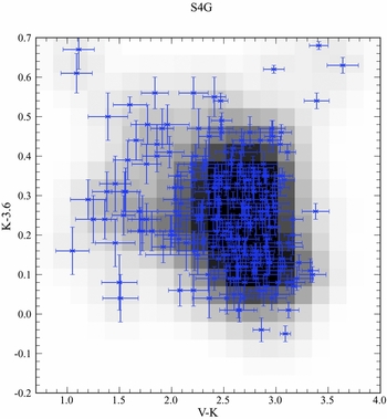
The largest sample of galaxies with both optical and Spitzer photometry is the Spitzer Survey of Stellar Structure in Galaxies project (S4G, Sheth et al. Reference Sheth, Regan and Hinz2010). We have combined the S4G photometry with B and V values from the RC3 (de Vaucouleurs et al. Reference de Vaucouleurs, de Vaucouleurs and Corwin1991) and K values from 2MASS (Jarrett et al. Reference Jarrett, Chester, Cutri, Schneider and Huchra2003, corrected for systematic bias, Schombert 2011). Culling the sample for galaxies with optical photometric errors less than 0.10 mags and near-IR errors less than 0.15 mags produced a final sample of 245 galaxies ranging in V mags from 12.5 to 7.
The resulting two color diagrams are shown in Figures 6 and 7 as both density distributions and individual data points with errorbars. The trend for bluer B − V for V − K colors is obvious, the curvature matches the behavior of the stellar population models (see Section 4.1). The relationship between K − 3.6 and V − K is very weak (R = 0.60) and such that bluer V − K colors predict redder K − 3.6 colors. The large scatter in color below V − K < 2.0 is more than likely due to dust emission contamination from the far-IR by the high SFR members of the S4G sample. A better representation of the data is simply that the mean K − 3.6 color is 0.27 ± 0.11 and we will be using this value to correct V − K colors into V − 3.6 for our models, although for high SFR galaxies a value of K − 3.6 between 0.4 and 0.5 is more realistic.
4 ANALYSIS
4.1 Photometric correction budget
The effect of the various population corrections as shown in Figure 8. The adopted MDF and chemical enrichment scenarios are assumed for the simulations and are considered variables to the final model results. All population corrections work to drive optical colors blueward, except for the influence from TP-AGBs which has no effect on blue optical colors. In the near-IR, the population corrections for BHBs and α/Fe effects are opposite to the corrections for TP-AGBs (although the TP-AGBs correction is twice the magnitude of the sum of the other corrections). The corrections shown in Figure 8 are adopted from LMC star cluster data, which represents a population with a mean [Fe/H] of − 0.5. Variation in luminosity with metallicity is approximately a factor of three from metal-poor to solar (Marigo & Girardi Reference Marigo and Girardi2007), but the short lifetimes for TP-AGBs excludes the lowest metallicities from our models. The metallicity of the LMC calibrating clusters is a close match the mean end metallicities of our models, variations in K luminosity up to 30% can be expected over the range of model metallicities which translates into a 0.03 variation in V − K color. For the purpose of the following discussion, we have adopted the red vector in Figure 8 as single linear correction to each simulation. Thus, one should consider the accuracy of the simulations to be limited by about 0.05 in optical colors and 0.07 in near-IR colors.
These corrections, while notable, are small compared to the combined effects of chemical evolution model and recent star formation. As can be seen in Figure 4, by the end of a constant star formation scenario the optical colors are dominated by the stellar populations from the last 0.5 Gyrs. The near-IR colors, on the other hand, would normally track along the optical colors, primarily influenced by the older metal-poor component from before 5 Gyrs and recent TP-AGBs.
The difference in B − V (bottom panel) and V − K (top panel) color for the single metallicity and the composite metallicity models. The push model represents a model which starts at [Fe/H] = −1.5 ending at solar following the curves in Figure 3. The large colors differences for the older ages is artificial in the sense that the push colors are for a much lower metallicity population and, thus, bluer colors. However, for the younger ages, the optical colors are dominated by young stars and the metal-poor portion of the underlying population has no effect. For near-IR colors, the age effects are less important compared to the temperature of the RGB, which has a strong contribution from metal-poor stars in the push model.

The black curve is the corrections to BC03 V − K colors from Marigo et al. (Reference Marigo, Girardi and Bressan2008), adopted from Maraston (Reference Maraston2005) and Bruzual & Charlot (Reference Bruzual and Charlot2003). The red curve is a 4th order polynomial fit to the model correction for smooth application to our simulations. A start time of 5 × 10⁷ yrs is assumed for the TP-AGB phase.
B − V versus V − K colors for 245 galaxies from the S4G sample (culled for small photometric errors). Error bars are shown and the underlying greyscale is a density plot of the sample.

V − K versus K − 3.6 colors for 245 galaxies from the S4G sample (culled for small photometric errors). Error bars are shown. In addition, a greyscale density distribution is also displayed where each data point is assumed to maintain a 2D gaussian with the XY errorbars defining the standard deviation. The frame is divided into series of pixels were the greyness of each pixel is based on the sum of each data points gaussian contribution to provide more definition in the concentrated regions. There is no correlation between V − K and K − 3.6, so a mean value of K − 3.6 = 0.27 is adopted to correct simulation K luminosities into 3.6 μ luminosities.
From these preliminary simulations, we know that, while including a multi-metallicity plus chemical enrichment model is important, small changes in the chemical enrichment scenario or the shape of the MDF have minor effects on those final colors. For example, adopting a gaussian MDF or a linear enrichment scheme only results in 0.005 mag difference in optical or near-IR colors. Optical colors were sensitive to the slope of the IMF at the high mass end, but again we have constraints on the upper end slope based on Hα measurements of LSB galaxy star clusters. The largest change in the model results from two variables; the star formation start epoch (i.e., the age of the first generation of stars) and the level of constancy to the star formation rate. Both to be discussed in the next sections.
4.2 Star formation history scenarios
As discussed in Section 1, the motivation for a constant star formation model was the discovery that the SFR for LSB galaxies, based on Hα emission, is such that the ratio of the current SFR to the total stellar mass is similar to a Hubble time. Star formation must be nearly constant in order to build up sufficient stellar mass, yet keep the stellar surface densities low. This is at the heart of the paradox to the appearance of LSB galaxies, for they require low mean star formation rates in order to keep their stellar densities low. However, low star formation rates produce red optical colors. The blue nature to LSB also require sufficient recent star formation to produce hot, young stars. Thus, a much larger past SFR, followed by quiescence till the present epoch, is inconsistent with their present-day optical colors.
For this reason, all the simulations start times were set to 12 Gyrs (assuming some small amount of time since the Big Bang for the galaxy to gravitationally collapse). The simulations were stepped forward in units of 10 Myrs which was shorter than the lifetime of the most massive star in our stellar tracks. With a 12 Gyrs formation epoch, the resulting color tracks for B − V and V − 3.6, as a function of metallicity, are shown in Figure 9 (the midline track). The displayed metallicity is the numerical average of the summed stellar populations of all ages, not a luminosity weighted value. We note that there are numerous galaxies with colors redder than our solar endpoint, indicating some super-solar metallicities exist in star forming galaxies. In addition, there are a number of galaxies with very blue V − 3.6 colors (V − 3.6 < 2) suggesting that the AGB component in those galaxies may be overestimated (V − 3.6 colors of 1.5 are produced by low metallicity models without any TP-AGBs).
Figure 9 displays the data for LSB galaxies (Schombert & McGaugh 2014), the S4G sample and a set of ellipticals from Dale et al. (Reference Dale, Bendo and Engelbracht2005). The S4G sample is divided into early-type (RC3 T < 4) and late-type (T > 4). The constant star formation model is shown as the solid line for various mean [Fe/H]. Also shown is a 12 Gyr SSP, which matches the elliptical data from Dale et al. (Reference Dale, Bendo and Engelbracht2005). The constant star formation model matches the mean LSB colors well and agrees with the color relation for the late-type S4G. The early-type S4G galaxies lie redward of the models, indicating the influence of a red bulge on their integrated colors.
It is important to remember that the final colors are independent of the SFR for a galaxy, as long as the rate is constant. Low SFR galaxies produce fewer stars than high SFR galaxies, but the proportion of light each generation is a constant fraction of the stellar mass. A high SFR galaxy will have a higher total luminosity (and they do, see Figure 10 in Schombert et al. Reference Schombert, Maciel and McGaugh2011), but the colors will be identical to a lower SFR galaxy. This explains the lack of any correlation between color and L Hα for many galaxy samples in the literature.
A scenario for completely constant star formation is only realistic if there is no variation in the star formation rate. It should be possible to constrain the adherence to a constant SF model for LSB galaxies by examining the amount of scatter (above observational error) in optical colors versus Hα flux. A more direct measure of the variation in the SFR is the scatter in the L Hα as a function of galaxy mass. This relationship (see Figure 10, Schombert et al. Reference Schombert, Maciel and McGaugh2011) displays a variation by a factor of 4 in L Hα (3σ) scatter from a linear relation (see also Lee et al. Reference Lee, Worthey and Dotter2009). As Hα emission is a measure of the SFR over short timescales, we can alter the constant star formation model to represent quasi-bursts of a factor of 4 intensity over the last 0.5 Gyrs (also shown in Figure 9). This 0.5 Gyrs timescale for bursts matches the HST analysis of dwarf galaxy CMD’s (McQuinn et al. Reference McQuinn, Skillman and Cannon2010). Numerical experimentation showed that bursts of this magnitude before 0.5 Gyrs fade quickly into the older population’s colors, so the burst only applies to the most recent, and most metal-rich, epoch. The application of a burst model to the models can be seen in Figure 9, where the burst models cover most of the spread in LSB colors, but the late-type S4G sample is better fit by the low burst (1/4x) scenario than the high burst (4x) one.
The constant star formation scenario for LSB galaxies was suggested by Figure 7 of Bell & de Jong (Reference Bell and de Jong2000), where there is a strong decrease in mean stellar population age with fainter surface brightness. Their interpretation is that stellar surface density maps into gas surface density such that lower LSB galaxies have lower SFR due to low gas densities. This also produces less chemical evolution and, thereby, low mean metallicities. Our models propose the same results, although we make no claim on the mechanism behind our scenarios.
The burst scenario is in agreement with the FUV results of Boissier et al. (Reference Boissier, Gil de Paz and Boselli2008). The FUV colors are most sensitive to recent star formation, and Boissier et al. find LSB galaxies have lower SFR than normal spirals (see also our Hα observations from Paper I). They also interpret the range in FUV-NUV colors of LSB galaxies as burst and quenching of recent star formation (on timescales of 100 Myrs). And, they also conclude that star formation is relatively constant on timescales of Gyrs, as our models also deduce. Thus, the important of UV and near-IR colors to map the SFH of LSB galaxies can not be overstated.
The median color line for the early-type S4G sample suggests that the current star formation rate is less than the past rate. This is in agreement with the birthrate estimates based on their gas supply, where the ratio of gas to stellar mass indicates more star formation in the past (McGaugh & de Blok Reference McGaugh and de Blok1997). To consider a scenario of declining star formation, we have take a mean birthrate function of 75% and adjusted the star formation to decline linearly from 12 Gyrs to the present. To match the birthrate function, this requires a change in the current star formation rate of 60% from the initial rate. This differs slightly from exponential star formation scenarios (Bell & de Jong Reference Bell and de Jong2000), but achieves approximately the same population at the end of the model. The resulting track is shown in Figure 10 using the same notation as Figure 9. The declining star formation model brackets the late-type S4G sample and explains a majority of the early-type spirals as well.
Lastly, we consider a different star formation start epoch, other than the assumed 12 Gyrs for the previous simulations. This is an old hypothesis that LSB galaxies are actually younger than other spirals or irregulars (McGaugh, Schombert, & Bothun Reference McGaugh, Schombert and Bothun1995). To this end, we simply changed the start time for the simulations in increments of Gyrs from 12 to 5 Gyrs. The results were remarkable consistent in that there is some change in V − 3.6 and a majority of the shift is in B − V. The color change was linear until approximately 6 Gyrs with a shift of Δ(B − V) = −0.01 per Gyrs and a shift of Δ(V − 3.6) = −0.005 per Gyr. This rapidly rules out any normal or HSB spiral as being less than 12 Gyrs in age, a result known for decades (Tully, Mould, & Aaronson Reference Tully, Mould and Aaronson1982). However, populations of ages between 10 and 12 Gyrs, for S4G and LSB galaxies, can not be ruled out by the data.
4.3 Mass-to-light ratios
As noted in McGaugh & Schombert (2014), many commonly employed models fail to provide self-consistent results with respect to the M/L values in galaxies. The stellar mass estimated from the luminosity in one band can differ grossly from that of another band for the same galaxy. Independent models agree closely in the optical, but diverge at longer wavelengths.
The tension in M/L values from population models is due to the competing contributions of mass from numerous, older, low mass stars and the high luminosity from new, hotter stars. The style of star formation is critical to the evolution of M/L as recent star formation reduces the contribution from older stars, and increasing the flux from high mass stars resulting in a lower observed value for M/L.
For our simulations, the shape of the lower end of the IMF effectively ties the mass of the populations for the upper mass end of the IMF, which contains the bluest stars, are a negligible component to the total mass of the population. While we have good constraints on the upper end of the IMF for LSB galaxies, from the correlation between optical luminosity and L Hα, the colors of LSB galaxies are dominated by both high mass and evolved stars, and do not give us constraints on the low mass end of the IMF. While we have no reason to believe that the IMF of LSB galaxies differs from the standard IMF at the low mass end, this will be the largest uncertainty in our M/L predictions.
The driving factors for the luminosity in M/L will be wavelength dependent. For the optical colors, luminosity in M/L is dominated by very blue, short-lived high mass stars. For near-IR color, the luminosity component is sensitive to TP-AGBs, which have longer lifetimes than high mass stars, but whose contribution can vary with small increases/decreases in recent star formation (i.e., bursts). Here we can be guided by the match between the models and the galaxy colors in Figures 9 and 10 which is quite good.
The resulting M/L tracks for our constant, burst and declining SF models (as discussed in Section 4.2) are shown in Figure 11 as a function of V − 3.6 color. Here the bluest colors are the lowest metallicity models ([Fe/H] = − 1.5) and the reddest colors are models with super-solar metallicity. As suspected from early models (Bell & de Jong Reference Bell and de Jong2001; Bell et al. 2003; Portinari, Sommer-Larsen, & Tantalo Reference Portinari, Sommer-Larsen and Tantalo2004; Zibetti, Charlot, & Rix Reference Zibetti, Charlot and Rix2009; Into & Portinari Reference Into and Portinari2013), the change in M/L with metallicity is effectively zero for far-IR colors such that if the star formation rate is known, the resulting M/L is a constant value for a range of total metallicities (i.e., galaxy mass). However, the zeropoint for each model varies from scenario to scenario. This is also expected since the primary variable for each model is the gas consumption rate. Models loaded with early star formation produce high M/L values and M/L decreases as the star formation becomes more constant with time. The low and high burst models also capture the same behavior since the value of M * is constant at late epochs, but the value of L increases or decreases sharply from enhanced or depressed star formation in the last 0.5 Gyrs.
To demonstrate the importance of determining which star formation scenario is appropriate, we have plotted the S4G sample M/L estimates from Zaritsky et al. (2014) using the prescription of Eskew, Zaritsky, & Meidt (Reference Eskew, Zaritsky and Meidt2012). Here the M/L values are determined empirically from the relation between stellar mass to L 3.6 in the LMC (extrapolating by a factor of 1000 from clusters with 107 M ⊙ to galaxy masses). The range of M/L is limited due to the lack of strong correlation between cluster mass and 3.6 or 4.5 μm colors, thus the stellar mass is simply a linear function of 3.6 luminosity resulting in a constant M/L of 0.52 ± 0.07. The constant SF model produces a range of M/L from 0.41 to 0.55 with a mean value of 0.45. The average M/L from the S4G sample is 20% higher than the constant SF model M/L, but less than the declining star formation model (mean M/L=0.82), which is a better fit to the S4G colors.
Also shown in Figure 11 are the M/L estimates from McGaugh & Schombert (2014) using the baryonic Tully-Fisher relation to estimate the stellar mass from the baryonic mass minus the gas mass. The mean value for that sample is M/L = 0.45 ± 0.15, in close agreement with the same models that reproduce LSB colors. As argued in McGaugh & Schombert (2014), and supported by the models herein, assuming a constant M/L as using the 3.6 luminosity of a galaxy results in the most accurate, and repeatable, stellar mass estimate.
5 CONCLUSIONS
LSB galaxies represent a unique opportunity in stellar population modeling for their low current star formation rates mean that their colors are not completely dominated by the most recent episode of star formation. In addition, their low metallicities and stellar densities minimises complicates due to dust and gas extinction. Their gas fractions and stellar mass to SFR ratios limit the range of star formation history paths to one that is basically constant star formation for the entire life of the galaxy.
We summarise our model results as the following:
-
(1) The primary difference between our current set of stellar population models and previous work is 1) using a full multi-metallicity treatment of the underlying population, 2) adopting a realistic chemical evolution model and IMF and 3) including corrections for α/Fe, BHBs, BSs and TP-AGBs effects. The error budget is displayed in Figure 8, only TP-AGB stars have a significant component, and only in the near-IR colors. Using Spitzer observations, we can extend the model colors to 3.6 μm from correlations between K and 3.6.
Figure 8.The various population corrections outlined in Section 4.1. A majority of the corrections drive galaxy colors blueward except for TP-AGBs which have a large near-IR redward correction. The corrections vary slightly with metallicity (becoming smaller with increasing metallicity). The adopted mean correction is shown as the red vector. All these corrections are minor compared to the shifts due to using a chemical enrichment model and the dominance of young stars.

-
(2) As demonstrated with ellipticals (Rakos & Schombert 2009), simple stellar populations (SSP’s) of a single metallicity are inadequate to describe galaxy colors. Applying a metallicity distribution function to a range of SSP’s allows one to construct a multi-metallicity composite population that merges the colors and luminosities of a range of stellar metallicities at a particular age.
-
(3) The present day colors of LSB galaxies can be modeled by a constant star formation scenario where the time of initial star formation is assumed to be 12 Gyrs. Each generation is assigned a mean metallicity to its MDF by following a standard chemical evolution prescription. The only free parameter is the final [Fe/H] value of this chemical evolution model, basically a proxy for the mean SFR as it reflects into the mean SN rate. The resulting track as a function of total galaxy metallicity is shown in Figure 9.
-
(4) Due to the constant star formation aspect of our models, only the shape of the upper IMF contributes to present-day colors and luminosities. We have solid constrains on the upper end of the IMF in LSB galaxies based on the correlation between star cluster luminosity and Hα fluxes (Schombert et al. Reference Schombert, McGaugh and Maciel2013). We note that uncertainties in the lower mass end of the IMF will only contribute to the uncertainty in model M/L estimates.
-
(5) Two other SF scenarios are considered, quasi-bursts and a declining star formation. The burst scenarios are where the star formation proceeds in a quasi-constant fashion with increases/decreases of star formation of a factor of four over 0.5 Gyrs timescales. This represents the range in scatter for the galaxy luminosity versus L hα relation. The second scenario to let the initial star formation to be significantly higher than the current SFR, then allow the SFR to decrease in a linear fashion to today’s rate. This overproduces the amount of stellar mass in older stars and reddens colors.
-
(6) The early-type spirals in the S4G sample are not well fit by the constant star formation model (being too red in optical colors). A declining star formation model, were the current star formation is 60% of the past average, is adequate to explain their optical and near-IR colors, although a range of percentages can be fit to the individual data points. None of the scenarios match S4G or LSB colors is the formation epoch is decreased by more than 2 Gyrs.
-
(7) The constant star formation model predicts constant M/L 3.6 in agreement with previous results using the baryonic Tully-Fisher relations (McGaugh & Schombert 2014). The model and baryonic TF mean M/L is 0.45, which is only 20% lower than the mean M/L from LMC clusters given the large statistical uncertainties (Eskew et al. Reference Eskew, Zaritsky and Meidt2012).

The two color, B − V vs V − 3.6 diagram for ellipticals (red stars), S4G early-type galaxies (red crosses), S4G late-type galaxies (blue crosses) and LSB galaxies (blue diamonds). A 12 Gyr multi-metallicity model is shown as a solid line passing through the elliptical data. The midline track through the S4G sample represents the constant star formation scenario with all the population corrections discussed in the text. The simulations ranged from [Fe/H] = −1.5 to solar. Parallel to the constant star formation track are the low and high burst scenarios where the level of star formation is increased or decreased by a factor of 4 for the last 0.5 Gyrs of the simulation. This covers the range of burst estimates from Lee et al. (Reference Lee, Worthey and Dotter2009) and McQuinn et al. (Reference McQuinn, Skillman and Cannon2010). A majority of the star forming galaxies are in agreement with the constant SF model.

The same as Figure 9 where the displayed models represent a declining star formation scenario where the SFR is decreased in a linear fashion to 60% of the initial star formation rate. The scenario accounts for a majority of the early-type galaxies in the S4G sample.

The relationship between M/L 3.6 and galaxy color (V − 3.6). The models for constant SF (black line, extended to redder colors), declining SF (red line) and a burst model (blue line). The bluest colors represent the lowest metallicities ([Fe/H]= − 1.5) and solar metallicity is approximately V − 3.6 = 3.0. In comparison, the M/L data from Zaritsky et al. (2014) is shown (red symbols) and M/L estimates from the baryonic TF relation (blue symbols, McGaugh & Schombert 2014). The mean M/L estimate of 0.45 from McGaugh & Schombert is shown as the dotted line.

The motivation for this set of models is the high gas fractions in LSB galaxies and should have limited application for HSB galaxies or early-type morphologies. Figure 9 would support this conclusion as the colors of most of the S4G sample are redder than the models. The models do predict the colors of LSB galaxies, and a substantial fraction of the late-type S4G galaxies. Small modifications to the constant star formation assumption, for example a slightly declining star formation rate, recovers the most of the colors of early-type spirals, but without uniqueness to the predicted SF history.
These models illuminate many of the paradoxical features to LSB galaxies. Low current star formation rates are in agreement with their low stellar densities. Their blue optical colors can be reconciled with low stellar densities if the star formation has been constant or in a weak burst fashion. The models rule out the conclusion that LSB galaxies are “young”, in the sense that their epoch of initial star formation is recent, requiring ages of at least 10 Gyrs. The models tolerate a difference in formation age of 2 Gyrs between HSB and LSB galaxy population, but strongly rule out any difference greater than 5 Gyrs. Additional understanding of the stellar populations in LSB galaxies will required high resolution imaging of a few nearby LSB galaxies with HST, the topic of the fifth paper in our series.
ACKNOWLEDGEMENTS
Software for this project was developed under NASA’s AIRS and ADP Programs. This work is based in part on observations made with the Spitzer Space Telescope, which is operated by the Jet Propulsion Laboratory, California Institute of Technology under a contract with NASA. Support for this work was provided by NASA through an award issued by JPL/Caltech. Other aspects of this work were supported in part by NASA ADAP grant NNX11AF89G and NSF grant AST 0908370. This research has made use of the NASA/IPAC Extragalactic Database (NED) which is operated by the Jet Propulsion Laboratory, California Institute of Technology, under contract with the National Aeronautics and Space Administration.


