

1. Introduction
The practice of the “Bank of Mum and Dad,” where parents assist their children in purchasing homes, is becoming increasingly common worldwide due to factors such as rising house prices, higher interest rates, and tighter lending restrictions. In the United States, 12% of home buyers relied on down payment help from friends and family as of April 2024 (Bhattarai and Cocco, Reference Bhattarai and Cocco2024). The youngest buyers – ages 25 to 33 years – were the most likely to receive help, with nearly 1 in 4 receiving cash gifts or loans. In Canada, the share of first-time home buyers who received help from family members was just under 30% in 2020, with the average gift being C$82,000 (Tal, Reference Tal2021). In Australia, the “Bank of Mum and Dad” ranks among the top ten mortgage lenders, with parents in New South Wales providing A$92,000 per adult child on average toward a deposit (Wootton, Reference Wootton2023). In the United Kingdom, around 16% of adults who move into homeownership receive an average gift of £20,000 from family and friends (Boileau and Sturrock, Reference Boileau and Sturrock2023).
Parents wanting to support their children (or grandchildren) financially face complex decisions that involve balancing this support with their own financial needs over a potentially long retirement period. These decisions include the form of support (e.g., gift or loan), the timing of the support (e.g., inter vivos gift or bequest) and the source of funding (e.g., financial assets or housing wealth). While many parents support their children using financial assets, in several countries, including the United States, the United Kingdom, and Australia, they can also use home equity release products, such as reverse mortgages, to access the wealth in their home, which is often the parents’ largest asset. Reverse mortgages are deferred payment loans that allow older homeowners to age in place and receive an income stream or lump sum payments secured against their homes. Previous studies (e.g., Davidoff, Reference Davidoff2010; Hanewald et al., Reference Hanewald, Post and Sherris2016) show that reverse mortgages can play an important role in retirement consumption smoothing. Conventional home equity borrowing products, such as home equity lines of credit or cash-out refinancing, require borrowers to demonstrate sufficient income to service regular repayments and are therefore typically unavailable to retirees with low or fixed income. Reverse mortgages do not require regular repayments and include features such as the no negative equity guarantee (NNEG) and strong occupancy rights, with loan proceeds that can support home-based care. These features make them particularly suitable for asset-rich, income-poor retirees. Reverse mortgages also enable parents to provide ‘early bequests’ and increase the certainty of the timing and size of (early) bequests (Merton, Reference Merton2007; Dillingh et al., Reference Dillingh, Prast, Rossi and Brancati2017). Two advantages of early bequests are that the parent can observe their child benefiting financially from the gift, while the adult child can use the funds earlier rather than waiting for an uncertain bequest later in life.
This paper presents a new two-generation lifecycle simulation model to study the consumption, housing and bequest decisions of families. We model the decisions many families face, where home-owning parents can decide to support their adult children in purchasing their first home. The new two-generation lifecycle simulation model differs from previous lifecycle models used to study consumption and housing decisions (e.g., Nakajima and Telyukova, Reference Nakajima and Telyukova2017; Shao et al., Reference Shao, Chen and Sherris2019; Koo et al., Reference Koo, Pantelous and Wang2022) in two important ways: (i) it captures the decisions of a home-owning parent and their adult child and considers both the parent and child’s lifetime expected utility, and (ii) it incorporates altruism by assuming that the parent derives utility from both the child’s utility in the same period and the child’s expected future utility after the parent’s death. Additionally, the model captures factors such as house price risk, interest rate risk, investment risk, wage growth, health shocks and associated long-term care costs, means-tested public pensions and private pensions, as well as relevant taxes, fees, and policies surrounding gifting and retirement planning.Footnote 1 Given the high-dimensional state space implied by the two-generation structure and the rich economic and institutional features of the model, we adopt a scenario-based approach with optimized consumption targets under each scenario rather than a fully structural dynamic programming framework. This allows us to preserve these features while maintaining tractability. While our model is calibrated using Australian socioeconomic, health, and market data and reflects the Australian pension system, our results are informative for other markets, and the two-generation framework can be easily applied to other countries.
We use the model to compare and analyze two key decisions for home-owning parents: whether to access home equity via a reverse mortgage and whether to provide an inter vivos gift or leave a larger bequest. We perform a scenario analysis to quantify the impact of these decisions on the lifetime expected utility of parents and children across the wealth distribution. The model results indicate that families in all wealth quartiles can experience welfare gains by using a reverse mortgage to supplement parental retirement income and fund a child’s first home deposit. Furthermore, early bequests result in much higher aggregate utility gains for the family compared to the parent only using the reverse mortgage to increase their retirement income, with the exception of cases where the parent is in the lowest wealth quartile and the child is in the highest. By incorporating parental altruism instead of a standard bequest utility function, our model captures the positive impact of early bequests on both parent and child. We also present a policy experiment where we study the impact of different pension rules for inter vivos gifts.
Our study adds to the growing literature on reverse mortgages by modeling their impact on consumption and housing for both generations, while also exploring the relationship that reverse mortgages can have on bequest motives and inter vivos transfers. Previous studies have explored the demand for reverse mortgages using one-generation lifecycle models for single or coupled retirees, with most focusing on the United States (e.g., Davidoff, Reference Davidoff2009, Reference Davidoff2010; Nakajima and Telyukova, Reference Nakajima and Telyukova2017; Cocco and Lopes, Reference Cocco and Lopes2020; Achou, Reference Achou2021), and only a few on other countries such as Canada (Michaud and Amour, Reference Michaud and Amour2023) or Australia (Andréasson and Shevchenko, Reference Andréasson and Shevchenko2024; Koo et al., Reference Koo, Pantelous and Wang2022). These structural models generally predict a higher demand for reverse mortgages among individuals with weaker bequest motives, lower levels of financial wealth relative to housing wealth, and higher levels of preexisting debt (Mayer and Moulton, Reference Mayer and Moulton2022). However, reverse mortgage markets are small internationally, and several studies investigate factors explaining this “reverse mortgage puzzle” – the mismatch between predicted demand and observed low take-up rates. Empirical studies, mostly survey based, find that low reverse mortgage demand is due to factors such as high costs, aversion to debt, and a lack of understanding of the product (e.g., Davidoff et al., Reference Davidoff, Gerhard and Post2017). The empirical findings on bequest motives are mixed: some studies suggest that bequest motives reduce reverse mortgage demand (Davidoff et al., Reference Davidoff, Gerhard and Post2017; Hanewald et al., Reference Hanewald, Bateman, Fang and Wu2020), while others find the opposite (Choinière-Crèvecoeur and Michaud, Reference Choinière-Crèvecoeur and Michaud2023). Dillingh et al. (Reference Dillingh, Prast, Rossi and Brancati2017) found that the most influential factor reducing interest in reverse mortgage products is having grand(children), which diminishes interest in reverse mortgages by 30%. However, providing examples of reverse mortgage use for the benefit of the homeowners’ (grand)children significantly raises interest in reverse mortgages among people with a bequest intention, which Dillingh et al. (Reference Dillingh, Prast, Rossi and Brancati2017) interpreted as evidence that people are unaware of the potential of reverse mortgages to optimize the timing of wealth transfers. Our study intends to quantify the welfare benefits of this precisely using our lifecycle simulation model, which is driven by a historically calibrated economic scenario generator of 13 key economic stochastic variables.
Thus, our study provides new insights into the factors influencing reverse mortgage demand and highlights an opportunity for providers to increase awareness of the “gifting function” of reverse mortgages. This could benefit both retirees and reverse mortgage providers by helping families optimize their housing wealth while addressing concerns about bequests. Previous one-generation models suggested that stronger bequest motives reduce reverse mortgage demand but overlook the role of early bequests and altruistic parents. Our findings show that parents can provide their children with a 20% home deposit with minimal impact on their own consumption, offering a viable alternative to traditional bequests. A policy experiment quantifying the impact of removing gifting limits on Australian Age Pension eligibilityFootnote 2 shows that lifting these limits primarily affects middle-wealth families, reducing welfare gains by less than 2.3%. However, given the much larger welfare gains from gifting, the overall impact of gifting limits is small, as they only affect pensioners near the Age Pension asset test thresholds and apply for at most five years. Our modeling framework is applicable to other retirement systems, including those in the United States and United Kingdom, where defined contribution savings, high housing wealth, public pensions, and gifting policies shape retirement decisions.
The remainder of the paper is organized as follows: Section 2 introduces the new two-generation lifecycle simulation model. Section 3 presents the simulation results and discusses their implications. Section 4 provides a sensitivity analysis, followed by concluding remarks in Section 5.
2. Two-generation lifecycle simulation model
In this section, we propose a new two-generation discrete-time lifecycle simulation model to study the consumption, housing, and bequest decisions of families. The model adopts a scenario-based approach with optimized consumption targets for each scenario and extends previous literature by representing a retired homeowning parent and their non-homeowning adult child. It considers both the parent’s and child’s lifetime expected utility and incorporates altruism, where the parent derives utility from the child’s current utility as well as the child’s expected future utility after the parent’s death. The model can be easily applied to other household types, such as coupled parents or multiple adult children, by increasing the number of health states and children modeled, including extensions to further generations.
We apply the model to the Australian retirement income system, which comprises a means-tested public pension called the Age Pension and private savings in the so-called superannuation system. Individuals receive the Age Pension if their “means,” that is, their assets and income, are below certain thresholds. As a result, Australian retirees can either receive the full Age Pension, a part Age Pension, or be “self-funded”. The owner-occupied home is exempt from the Age Pension assets test. Appendix B provides more details on the Age Pension and its means-tested calculations, including gifting limits under the assets test. The tax-preferred superannuation system mandates employer contributions (currently 12% of wages) into individual retirement accounts, which offer investment choices. Upon retirement, individuals can access their superannuation savings as a lump sum or as an income stream, subject to age-specific minimum drawdown rates. Most Australians convert their superannuation savings to account-based pensions, which are investment accounts that provide flexible withdrawals but do not offer longevity risk protection. The demand for annuities is low. The model captures all of these aspects, along with aged care costs and means-tested government assistance for aged care. We also model commercial reverse mortgages available in Australia.Footnote 3
In summary, the model accounts for house price risk, interest rate risk, investment risk, wage growth, health shocks and associated long-term care costs, means-tested public pensions, as well as relevant taxes, fees, and policies for gifting and retirement planning. Five health states are modeled for each generation and calibrated to match 2018 data from the Survey of Disability, Ageing and Carers (SDAC) from the Australian Bureau of Statistics. Simulations and results are based on realistic forecasts of key economic variables using an economic scenario generator (Chen et al., Reference Chen, Koo, Wang, O’Hare, Langrené, Toscas and Zhu2021), which we apply to model housing and wealth decisions for a single parent and adult child across a range of wealth levels. All variables and parameters are set at the start of the 2022 financial year (FY2022) and are defined in real terms, adjusted for inflation.Footnote 4 We estimate initial wealth and income levels from the latest wave of data collected by the nationally representative Household, Income and Labour Dynamics in Australia (HILDA) Survey. The HILDA Survey is a household-based longitudinal study of approximately 9,000 households, first administered in 2001. Every four years, the survey includes a wealth module, with the latest included in Wave 22 for 2022.
2.1. Utility framework
We start by developing a utility-based framework suitable for studying decisions about consumption, housing, bequests, and the use of reverse mortgages as a tool for early bequests. The model structure is inspired by two-generation models used to study long-term care insurance decisions by older parents with adult children, who can either provide informal long-term care or participate in the labour force (e.g., Klimaviciute et al., Reference Klimaviciute, Pestieau and Schoenmaeckers2019, Reference Klimaviciute, Pestieau and Schoenmaeckers2020; Ko, Reference Ko2022; Mommaerts, Reference Mommaerts2025; Zweifel and Strüwe, Reference Zweifel and Strüwe1998). However, instead of studying long-term care decisions, our new model focuses on housing wealth, early bequest and reverse mortgage decisions and models utility from consumption and housing. Our model extends the literature by modeling the impact of reverse mortgages for a two-generation family, with the option to gift the child an early bequest. We also clearly quantify the differences in welfare gains between models that consider parent bequest utility, which is commonly used in the retirement modeling literature, versus parental altruism. Mukherjee (2022) has recently shown that pure altruistic preferences play a significant role in retirement transfers, with parents passing on additional income via inter vivos gifts, without receiving any additional care in return. By studying the impact of parental altruism on reverse mortgage decisions, we show that as the parent cares more about their child’s well-being, the possible benefits from reverse mortgages increase.
The parent gains utility at time t from consumption $C^P(t)$
, housing
$C^P(t)$
, housing $H^P(t)$
, and her child’s utility as follows:
$H^P(t)$
, and her child’s utility as follows:
 \begin{equation}U^{P}(t) = I^{P,A} (t) \cdot \left( U(C^{P}(t), H^P(t)) + \rho \cdot U^{C}(t) \right) + I^{P,D}(t) \cdot \rho \cdot V^C ( T^{P} ),\end{equation}
where $T^P$
is the time of the parents death,
$T^P$
is the time of the parents death, $I^{P,A} (t) $
is an indicator variable that equals one when the parent is alive and zero otherwise,
$I^{P,A} (t) $
is an indicator variable that equals one when the parent is alive and zero otherwise, $I^{P,D} (t)$
is an indicator variable that equals one only in the period when the parent dies and 0 otherwise, and
$I^{P,D} (t)$
is an indicator variable that equals one only in the period when the parent dies and 0 otherwise, and $\rho$
is an altruism parameter that controls the importance of the adult child’s happiness to the parent. When the parent is alive
$\rho$
is an altruism parameter that controls the importance of the adult child’s happiness to the parent. When the parent is alive $(t \lt T^P)$
, she gains utility
$(t \lt T^P)$
, she gains utility $\rho \cdot U^{C} (t)$
from the child’s utility in the same period. In the period when the parent dies
$\rho \cdot U^{C} (t)$
from the child’s utility in the same period. In the period when the parent dies $(t = T^P)$
, the parent gains utility
$(t = T^P)$
, the parent gains utility $\rho \cdot V^C (T^{P})$
based on the total expected utility of the adult child after the parent’s deathFootnote
5
, which is defined by
$\rho \cdot V^C (T^{P})$
based on the total expected utility of the adult child after the parent’s deathFootnote
5
, which is defined by
 \begin{equation} V^C (T^{P}) = E_{T^{P}} \left[\sum_{t=T^{P}}^{T^{C}} \beta^{(t-T^{P})} U^C (t) \right],\end{equation}
where $T^C$
is the child’s time of death,
$T^C$
is the child’s time of death, $E_t$
represents the conditional expectation based on information up to time t, including realized economic variables from the economic scenario generator and any health state transitions, and
$E_t$
represents the conditional expectation based on information up to time t, including realized economic variables from the economic scenario generator and any health state transitions, and $\beta$
denotes the subjective discount factor.
$\beta$
denotes the subjective discount factor.
The adult child gains utility at time t from both her consumption $C^C (t)$
and housing
$C^C (t)$
and housing $H^C (t) $
, and from leaving a bequest,
$H^C (t) $
, and from leaving a bequest, $W^C(t)$
, to her own child in a third generation which is not modeled:
$W^C(t)$
, to her own child in a third generation which is not modeled:
 \begin{equation}U^{C} (t)= I^{C,A} (t) \cdot U(C^{C} (t), H^C (t) ) + I^{C,D} (t)\cdot \theta \cdot B(W^{C} (t)),\end{equation}
where $I^{C,A} (t)$
is an indicator variable that equals one when the child is alive and zero otherwise,
$I^{C,A} (t)$
is an indicator variable that equals one when the child is alive and zero otherwise, $I^{C,D} (t)$
is an indicator variable that equals one only in the period when the child dies and zero otherwise,
$I^{C,D} (t)$
is an indicator variable that equals one only in the period when the child dies and zero otherwise, $\theta$
is the bequest utility weight, which can be different from the parent’s altruism parameter.
$\theta$
is the bequest utility weight, which can be different from the parent’s altruism parameter.
Since the third generation is not modeled, we cannot apply an altruistic utility framework for the child because the grandchild’s consumption, housing, and wealth outcomes are not specified. As we only model the bequest left by the child, we assume the child’s bequest utility function, B follows a standard constant relative risk aversion (CRRA) form:
 \begin{equation} B(W (t) ) = \frac{{W(t)^{1-\gamma}}}{{1-\gamma}},\end{equation}
where $\gamma\gt1$
is the relative risk aversion parameter. The period utility function for both the parent and adult child is given by a Cobb–Douglas utility function for consumption and housing, which has been widely used in models involving the optimal use of housing wealth with a reverse mortgage (e.g., Nakajima and Telyukova, Reference Nakajima and Telyukova2017; Shao et al., Reference Shao, Chen and Sherris2019). It is a straightforward and versatile utility function, allowing for flexible substitution between consumption and housing while ensuring proportional allocation to both goods as wealth increases:
$\gamma\gt1$
is the relative risk aversion parameter. The period utility function for both the parent and adult child is given by a Cobb–Douglas utility function for consumption and housing, which has been widely used in models involving the optimal use of housing wealth with a reverse mortgage (e.g., Nakajima and Telyukova, Reference Nakajima and Telyukova2017; Shao et al., Reference Shao, Chen and Sherris2019). It is a straightforward and versatile utility function, allowing for flexible substitution between consumption and housing while ensuring proportional allocation to both goods as wealth increases:
 \begin{equation} U(C (t),H (t)) = \frac{{(C(t)^{\eta} (\delta_i H(0))^{1-\eta})^{1-\gamma}}}{{1-\gamma}},\end{equation}
where $\eta \in [0,1)$
denotes the share of consumption in the Cobb–Douglas aggregator. Note that the same relative risk aversion parameter is used in U and B to ensure consistency in risk preferences across different sources of utility and to maintain tractability by allowing bequests to be interpreted as deferred consumption.
$\eta \in [0,1)$
denotes the share of consumption in the Cobb–Douglas aggregator. Note that the same relative risk aversion parameter is used in U and B to ensure consistency in risk preferences across different sources of utility and to maintain tractability by allowing bequests to be interpreted as deferred consumption.
Utility from housing is based on an “imputed rent,” calculated as a fixed proportion $\delta_i$
of the initial home value
$\delta_i$
of the initial home value $H_0$
, following Shao et al. (Reference Shao, Chen and Sherris2019). We assume
$H_0$
, following Shao et al. (Reference Shao, Chen and Sherris2019). We assume $\delta_i$
to be two possible values (based on Shao et al., Reference Shao, Chen and Sherris2019), satisfying
$\delta_i$
to be two possible values (based on Shao et al., Reference Shao, Chen and Sherris2019), satisfying
 \begin{equation} \delta_i = \left\{\begin{array}{lr} \delta_1 = 5\%, & \text{before living in aged care},\\ \delta_2 =2.5\%, & \text{if living in aged care},\\ \end{array}\right.\end{equation}
based on the assumption that retirees still receive housing consumption when living in an aged care facility, but at a proportional rate to account for living conditions that are not as good as ageing in place or living in their own home throughout retirement. As such, housing consumption when in an aged care facility is not related to the actual aged care fees paid by the parent and child, which we define in Section 2.6. If the adult child is a non-homeowner and pays rent, then we estimate the initial home value $H_0^C$
based on her initial rent paid divided by a fixed annual rental yield of 5%.
$H_0^C$
based on her initial rent paid divided by a fixed annual rental yield of 5%.
We assume that consumption is nonnegative in each period and that bequest wealth is also nonnegative.Footnote 6 We also do not allow for borrowing other than reverse mortgage borrowing for the parent and conventional mortgage borrowing for the adult child’s home.
The total lifetime expected utility for the parent ( $V^P$
) and the adult child (
$V^P$
) and the adult child ( $V^C$
) are given by
$V^C$
) are given by
 \begin{equation}V^P= E_0\left[\sum_{t=0}^{T^{P}} \beta^t U^P (t) \right] \text{and} \; V^C= E_0\left[\sum_{t=0}^{T^{C}} \beta^t U^C (t) \right].\end{equation}
The aggregate expected lifetime utility, V, is defined as the weighted sum of the parent and adult child’s lifetime expected utility:
 \begin{equation} V = \omega^PV^P+\omega^CV^C,\end{equation}
where the Pareto weights $ \omega^P $
and
$ \omega^P $
and $ \omega^C $
are chosen to normalize the parent’s and adult child’s lifetime expected utility to be of a similar magnitude. The adult child’s utility tends to be larger due to having a higher expected number of remaining years alive. These weights also reflect the relative importance of each generation’s utility in the aggregate welfare function. They can be adjusted to analyze different decision-making scenarios where the welfare of the parent or the adult child is given more significance. The Pareto weights are subject to the constraint:
$ \omega^C $
are chosen to normalize the parent’s and adult child’s lifetime expected utility to be of a similar magnitude. The adult child’s utility tends to be larger due to having a higher expected number of remaining years alive. These weights also reflect the relative importance of each generation’s utility in the aggregate welfare function. They can be adjusted to analyze different decision-making scenarios where the welfare of the parent or the adult child is given more significance. The Pareto weights are subject to the constraint: $ \omega^P + \omega^C = 1$
.
$ \omega^P + \omega^C = 1$
.
2.2. Model structure and timing
We now describe the model structure and timing. The model is defined over a series of one-year time periods, $t \in \{0, 1, 2, \ldots, T\}$
, which captures the parent’s and child’s decision at the start of each year. At time
$t \in \{0, 1, 2, \ldots, T\}$
, which captures the parent’s and child’s decision at the start of each year. At time $t=0$
, the parent is 67 years old (which is the minimum age for receiving the means-tested Age Pension in Australia) and retired. The parent owns a home, superannuation savings (mandatory, tax-preferred retirement savings), and financial and other assets (FOA).Footnote
7
The child is 36 years old, does not own a house, is employed full-time, and accumulates superannuation savings and FOA. At the start of each period, the parent and child receive income and consume up to an optimized consumption target depending on their wealth level (see Section 3.1). The parent can access their home equity via a reverse mortgage to supplement their retirement income and/or gift to the child for their first home deposit. While the parent and child are alive, they can be in one of four living health states (based on the disability and aged-care framework discussed in Section 2.6), each associated with out-of-pocket long-term care (LTC) costs (after accounting for means-tested government support). The health state is modeled by Markov processes
$t=0$
, the parent is 67 years old (which is the minimum age for receiving the means-tested Age Pension in Australia) and retired. The parent owns a home, superannuation savings (mandatory, tax-preferred retirement savings), and financial and other assets (FOA).Footnote
7
The child is 36 years old, does not own a house, is employed full-time, and accumulates superannuation savings and FOA. At the start of each period, the parent and child receive income and consume up to an optimized consumption target depending on their wealth level (see Section 3.1). The parent can access their home equity via a reverse mortgage to supplement their retirement income and/or gift to the child for their first home deposit. While the parent and child are alive, they can be in one of four living health states (based on the disability and aged-care framework discussed in Section 2.6), each associated with out-of-pocket long-term care (LTC) costs (after accounting for means-tested government support). The health state is modeled by Markov processes $G^P(t)$
and
$G^P(t)$
and $G^C(t)$
for the parent and child, respectively, taking states
$G^C(t)$
for the parent and child, respectively, taking states $\{1,2,3,4,5\}$
ranging from healthy (state 1) to deceased (state 5) and with associated transition probabilities.
$\{1,2,3,4,5\}$
ranging from healthy (state 1) to deceased (state 5) and with associated transition probabilities.
2.2.1. Parent
The parent’s state space at time t is defined by
 $$X^P(t) = \{ G^P(t), H^P(t), S^P(t), FOA^P(t), L^P(t) \},$$
where $G^P$
is the health state,
$G^P$
is the health state, $H^P$
is the house value,
$H^P$
is the house value, $S^P$
is superannuation wealth,
$S^P$
is superannuation wealth, $FOA^P$
is financial and other assets, and
$FOA^P$
is financial and other assets, and $L^P$
is the reverse mortgage loan balance. At time
$L^P$
is the reverse mortgage loan balance. At time $t=0$
, the parent retires in good health, thus
$t=0$
, the parent retires in good health, thus $G^P(0) = 1$
. Random death of the parent occurs at time
$G^P(0) = 1$
. Random death of the parent occurs at time $T^{P}$
, thus
$T^{P}$
, thus $G^P(T^{P}) = 5$
. Assuming a maximum age of 100, the parent’s time of death satisfies
$G^P(T^{P}) = 5$
. Assuming a maximum age of 100, the parent’s time of death satisfies $1 \leq T^{P} \leq 33$
.
$1 \leq T^{P} \leq 33$
.
While alive, the parent receives Age Pension entitlement $AP^P(t)$
, which is means-tested based on
$AP^P(t)$
, which is means-tested based on $X^P(t)$
and pays LTC fees
$X^P(t)$
and pays LTC fees $LTC^P(t)$
based on her realized health state
$LTC^P(t)$
based on her realized health state $G^P(t)$
.Footnote
8
The parent aims to consume a time-invariant consumption target
$G^P(t)$
.Footnote
8
The parent aims to consume a time-invariant consumption target $\bar{C}^P\gt0$
, which is optimized (see Section 3.1) based on their starting wealth quartile and assumed retirement decisions (e.g., whether to gift their child and/or use a reverse mortgage under the scenarios described in Section 2.7). Let
$\bar{C}^P\gt0$
, which is optimized (see Section 3.1) based on their starting wealth quartile and assumed retirement decisions (e.g., whether to gift their child and/or use a reverse mortgage under the scenarios described in Section 2.7). Let $C^P(t)$
denote the parent’s consumption and let
$C^P(t)$
denote the parent’s consumption and let $IA^P(t) = AP^P(t) - LTC^P(t) + S^P(t) + FOA^P(t)$
denote the income and liquid assets available at time t.Footnote
9
Then,
$IA^P(t) = AP^P(t) - LTC^P(t) + S^P(t) + FOA^P(t)$
denote the income and liquid assets available at time t.Footnote
9
Then,
 \begin{equation} C^P(t) =\begin{cases} \bar{C}^P, & \text{if } IA^P(t) \geq \bar{C}^P,\\ IA^P(t), & \text{if } IA^P(t) \lt \bar{C}^P.\end{cases}\end{equation}
In the worst case, if the parent runs out of liquid savings ( $S^P(t) = FOA^P(t) = 0$
), the parent is always able to consume the lesser of the optimized consumption target or Age Pension entitlement less LTC costs, thus
$S^P(t) = FOA^P(t) = 0$
), the parent is always able to consume the lesser of the optimized consumption target or Age Pension entitlement less LTC costs, thus $C^P(t) \geq \min(\bar{C}^P, AP^P(t) - LTC^P(t))$
.Footnote
10
The consumption and wealth dynamics are described by first defining the parent’s consumption shortfall,
$C^P(t) \geq \min(\bar{C}^P, AP^P(t) - LTC^P(t))$
.Footnote
10
The consumption and wealth dynamics are described by first defining the parent’s consumption shortfall, $\tilde{C}^P(t)$
, which denotes the amount that can be saved when negative (
$\tilde{C}^P(t)$
, which denotes the amount that can be saved when negative ( $\tilde{C}^P(t)\lt0$
) or must be withdrawn when positive (
$\tilde{C}^P(t)\lt0$
) or must be withdrawn when positive ( $\tilde{C}^P(t)\gt0$
) to reach the consumption target. Thus,
$\tilde{C}^P(t)\gt0$
) to reach the consumption target. Thus, $\tilde{C}^P(t)$
satisfies
$\tilde{C}^P(t)$
satisfies
 \begin{equation} \tilde{C}^P = \bar{C}^P - AP^P(t) - \alpha^S(t) S^P(t) + LTC^P(t).\end{equation}
where we assume the parent takes her superannuation as an account-based pension with a drawdown rate, $\alpha^S(t)$
, that is, consistent with the minimum age-based statutory rates. If
$\alpha^S(t)$
, that is, consistent with the minimum age-based statutory rates. If $\tilde{C}^P(t)\lt0$
, then the parent has sufficient savings and income to consume
$\tilde{C}^P(t)\lt0$
, then the parent has sufficient savings and income to consume $\bar{C}^P$
, and they deposit the surplus into FOA. If the parent has a consumption shortfall,
$\bar{C}^P$
, and they deposit the surplus into FOA. If the parent has a consumption shortfall, $\tilde{C}^P\gt0$
, they withdraw savings from FOA to achieve their target consumption,
$\tilde{C}^P\gt0$
, they withdraw savings from FOA to achieve their target consumption,
 \begin{equation} FOA^P(t+1) = \max \big\{FOA^P(t) - \tilde{C}^P(t), 0 \big\}\cdot \big(1 + r_F(t+1) \big),\end{equation}
where $r_F(t+1)$
is the investment return for FOA realized at the start of the next year and accounts for taxes on returns based on the parent’s taxable income from the Age Pension and investment returns (see Appendix D). If there are insufficient savings in FOA, i.e.,
$r_F(t+1)$
is the investment return for FOA realized at the start of the next year and accounts for taxes on returns based on the parent’s taxable income from the Age Pension and investment returns (see Appendix D). If there are insufficient savings in FOA, i.e., $FOA^P(t) \lt \tilde{C}^P(t)$
, then the parent withdraws from their account-based pension on top of the regulated minimum drawdown
$FOA^P(t) \lt \tilde{C}^P(t)$
, then the parent withdraws from their account-based pension on top of the regulated minimum drawdown $\alpha^S(t)$
. Thus,
$\alpha^S(t)$
. Thus,
 \begin{equation} S^P(t+1) = \max \big\{S^P(t) - \alpha^S(t) S^P(t) + \min(FOA^P(t) - \tilde{C}^P(t), 0),0\big\}\cdot\big(1 + r_S(t+1) \big),\end{equation}
where $r_S(t+1)$
is the investment return for the account-based pension realized at the start of the next year. No tax is paid based on the assumption that all superannuation was converted to an account-based pension at the start of retirement.Footnote
11
$r_S(t+1)$
is the investment return for the account-based pension realized at the start of the next year. No tax is paid based on the assumption that all superannuation was converted to an account-based pension at the start of retirement.Footnote
11
If the parent ever runs out of liquid assets to consume,
 $$ (1-\alpha^S(t)) S^P(t) + FOA^P(t) \lt \tilde{C}^P(t),$$
she can choose to use a reverse mortgage for additional income at any time to finance her own consumption target for the year. However, the parent’s reverse mortgage loan balance must always remain below the maximum age-specific loan-to-value ratios (LVR) set by the commercial reverse mortgage provider, in line with legal restrictions.Footnote
12
Let $LVR^{\max}(t)$
denote the maximum LVR for the parent at time t, then the parent borrows
$LVR^{\max}(t)$
denote the maximum LVR for the parent at time t, then the parent borrows
 \begin{equation} RM^P(t) = \min \big\{\tilde{C}^P(t) - (1-\alpha^S(t)) S^P(t) - FOA^P(t), LVR^{\max}(t)H^P(t) - L^P(t) \big\},\end{equation}
where $LVR^{\max}(t)H^P(t) - L^P(t)$
denotes the maximum amount the parent can borrow at time t based on their current reverse mortgage loan. If the parent has enough liquid assets, or if her LVR exceeds
$LVR^{\max}(t)H^P(t) - L^P(t)$
denotes the maximum amount the parent can borrow at time t based on their current reverse mortgage loan. If the parent has enough liquid assets, or if her LVR exceeds $LVR^{\max}(t)$
then
$LVR^{\max}(t)$
then $RM^P(t) =0$
. When including reverse mortgage dynamics,
$RM^P(t) =0$
. When including reverse mortgage dynamics, $IA^P(t)$
in Equation (9) can be replaced by
$IA^P(t)$
in Equation (9) can be replaced by $IA^P(t) = AP^P(t) - LTC^P(t) + S^P(t) + FOA^P(t) + \max(LVR^{\max}(t)H^P(t) - L^P(t),0)$
.
$IA^P(t) = AP^P(t) - LTC^P(t) + S^P(t) + FOA^P(t) + \max(LVR^{\max}(t)H^P(t) - L^P(t),0)$
.
For simplicity, the decision to gift the child a lump sum payment using the reverse mortgage is only considered at time $t=0$
. In this case, the parent borrows an additional lump sum
$t=0$
. In this case, the parent borrows an additional lump sum $\widetilde{RM}^P(0)$
as a gift to her child, based on a proportion,
$\widetilde{RM}^P(0)$
as a gift to her child, based on a proportion, $\alpha^{G}$
, of the child’s home,Footnote
13
satisfying
$\alpha^{G}$
, of the child’s home,Footnote
13
satisfying
 \begin{equation} \widetilde{RM}^P(0)= \min \big\{ \alpha^{G} H^C(0), LVR^{\max}(0)H^P(0) - L^P(0) \big\},\end{equation}
resulting in an initial loan of
 $$L^P(0) = RM^P(0)+\widetilde{RM}^P(0).$$
Upon the parent’s death or declining health and subsequent move into residential aged care, the house is sold in order to repay possible outstanding reverse mortgage loans and fund means-tested LTC costs such as the accommodation and daily care fees (which vary due to means-testing). We model the Australian downsizer contribution, which allows up to $300,000 from the sale of the home to be contributed into a superannuation account, with the remaining proceeds deposited into FOA. The sale of the home includes a $r_{HF} = 6\%$
fee to cover costs (Shao et al., Reference Shao, Hanewald and Sherris2015; Nakajima and Telyukova, Reference Nakajima and Telyukova2017). The loan and housing dynamics satisfies
$r_{HF} = 6\%$
fee to cover costs (Shao et al., Reference Shao, Hanewald and Sherris2015; Nakajima and Telyukova, Reference Nakajima and Telyukova2017). The loan and housing dynamics satisfies
 \begin{align} L^P(t+1) & = \big(L^P(t) + RM^P(t)\big) \cdot \big( 1+r_{RM}(t+1)\big), && \mbox{for $0\leq t \leq T^{P}-1$,}\end{align}
 \begin{align} H^P(t+1) & = H^P(t) \cdot ( 1+h(t+1)), && \mbox{for $0\leq t \leq T^{P} -1$,}\end{align}
where $r_{RM}(t)$
and h(t) are the reverse mortgage rate and house price growth rate, respectively. Both
$r_{RM}(t)$
and h(t) are the reverse mortgage rate and house price growth rate, respectively. Both $r_{RM}(t)$
and h(t) are defined in Section 2.3 based on a cascading structure of dependent autoregressive processes calibrated to historical Australian market data from 1992 to 2018 (see Chen et al., Reference Chen, Koo, Wang, O’Hare, Langrené, Toscas and Zhu2021). At time
$r_{RM}(t)$
and h(t) are defined in Section 2.3 based on a cascading structure of dependent autoregressive processes calibrated to historical Australian market data from 1992 to 2018 (see Chen et al., Reference Chen, Koo, Wang, O’Hare, Langrené, Toscas and Zhu2021). At time $t=T^{P}$
, when the parent dies, the parent bequests net assets
$t=T^{P}$
, when the parent dies, the parent bequests net assets $B^P(T^{P})$
satisfying
$B^P(T^{P})$
satisfying
 \begin{equation} B^P(t) = \max \{(1-r_{HF})H^P(t) - L^P(t),0 \} + S^P(t) + FOA^P(t),\end{equation}
where the first term reflects the NNEG included in Australian reverse mortgage loans, which ensures that the loan repayment does not exceed the proceeds from the sale of the home.
2.2.2. Child
The child’s state space at time t is defined by
 \[ X^C(t) = \{ G^C(t), W^C(t), H^C(t), S^C(t), FOA^C(t), L^C(t) \}, \]
where $G^C$
is the health state,
$G^C$
is the health state, $W^C$
is wages,
$W^C$
is wages, $H^C$
is the value of the house she rents or wishes to buy,
$H^C$
is the value of the house she rents or wishes to buy, $S^C$
is superannuation wealth,
$S^C$
is superannuation wealth, $FOA^C$
is financial and other assets, and
$FOA^C$
is financial and other assets, and $L^C$
is the child’s loan from a conventional mortgage (if applicable). At time
$L^C$
is the child’s loan from a conventional mortgage (if applicable). At time $t=0$
, we assume the child is employed, does not own a home, and pays taxes and rent. She remains healthy until retirement, and her random death occurs at time
$t=0$
, we assume the child is employed, does not own a home, and pays taxes and rent. She remains healthy until retirement, and her random death occurs at time $T^{C}$
, thus
$T^{C}$
, thus $G^C(T^{C}) =5$
, at which time the child gains utility from leaving a bequest to a third generation, which is not explicitly modeled. We assume a maximum age of 100 for the child,Footnote
14
and that she retires aged 67 years, the same retirement age as the parent. This implies the child retires at time
$G^C(T^{C}) =5$
, at which time the child gains utility from leaving a bequest to a third generation, which is not explicitly modeled. We assume a maximum age of 100 for the child,Footnote
14
and that she retires aged 67 years, the same retirement age as the parent. This implies the child retires at time $t=31$
and the child’s random time of death satisfies
$t=31$
and the child’s random time of death satisfies $32 \leq T^{C} \leq 64$
.
$32 \leq T^{C} \leq 64$
.
At time $t=0$
, the child purchases a home only if the parent immediately takes out a lump sum reverse mortgage and gifts her child a home deposit. The value of the house the child purchases
$t=0$
, the child purchases a home only if the parent immediately takes out a lump sum reverse mortgage and gifts her child a home deposit. The value of the house the child purchases $H^C(0)$
depends on her own wealth quartile and was estimated using the HILDA dataset, see Table 7. If the child purchases a home, she will stop paying rent
$H^C(0)$
depends on her own wealth quartile and was estimated using the HILDA dataset, see Table 7. If the child purchases a home, she will stop paying rent $R^C(t)$
and needs to repay her mortgage
$R^C(t)$
and needs to repay her mortgage $M^C(t)$
periodically based on a variable interest rate (see Section 2.3.1),
$M^C(t)$
periodically based on a variable interest rate (see Section 2.3.1), $r_M(t)$
. Assuming a typical variable-rate 30-year loan, the mortgage payments satisfy
$r_M(t)$
. Assuming a typical variable-rate 30-year loan, the mortgage payments satisfy
 \begin{equation} M^C(t) = L^C(t) \frac{r_M(t)(1+r_M(t))^{(30-t)}}{(1+r_M(t))^{(30-t)} -1},\end{equation}
for $0 \leq t\lt30$
, where
$0 \leq t\lt30$
, where $ L^C(t) $
is the remaining loan principal. The interest rate
$ L^C(t) $
is the remaining loan principal. The interest rate $ r_M(t) $
is modeled as the simulated cash rate plus a fixed lender margin. This formulation ensures that the loan is fully repaid by year 30 through real, annually updated payments. The mortgage payment
$ r_M(t) $
is modeled as the simulated cash rate plus a fixed lender margin. This formulation ensures that the loan is fully repaid by year 30 through real, annually updated payments. The mortgage payment $ M^C(t) $
is recalculated each year to reflect changes in the interest rate
$ M^C(t) $
is recalculated each year to reflect changes in the interest rate $ r_M(t) $
. To avoid complexity we assume that if the parent does not gift the child a home deposit, the child remains a non-homeowner and pays rent. We further assume that the annual rent is a fixed value
$ r_M(t) $
. To avoid complexity we assume that if the parent does not gift the child a home deposit, the child remains a non-homeowner and pays rent. We further assume that the annual rent is a fixed value $r^C_R$
dependent upon the wealth quartile of the adult child. As the model is discounted by the inflation rate and defined in real terms, rent is assumed to stay constant, thus growing only with inflation, in line with the same assumptions for the means-tested public pension and aged care support.
$r^C_R$
dependent upon the wealth quartile of the adult child. As the model is discounted by the inflation rate and defined in real terms, rent is assumed to stay constant, thus growing only with inflation, in line with the same assumptions for the means-tested public pension and aged care support.
The child’s consumption before retirement, where $t \lt 31$
, satisfies
$t \lt 31$
, satisfies
 \begin{equation}C^C(t) =\begin{cases}W^C(t) - R^C(t), & \text{if the child rents at time } t, \\W^C(t) - M^C(t), & \text{if the child owns a home with a mortgage at time } t,\end{cases}\end{equation}
where wages $W^C$
are subject to Australian tax laws, see Appendix D. This implies the child consumes all her wages each year after accounting for taxes, rent, or mortgage payments.Footnote
15
She will also receive the compulsory employer superannuation contributions to her superannuation account, which we assume to be 11% of gross wages, in line with laws in Australia at the time. Thus, for
$W^C$
are subject to Australian tax laws, see Appendix D. This implies the child consumes all her wages each year after accounting for taxes, rent, or mortgage payments.Footnote
15
She will also receive the compulsory employer superannuation contributions to her superannuation account, which we assume to be 11% of gross wages, in line with laws in Australia at the time. Thus, for $0\leq t \leq 30$
, we have
$0\leq t \leq 30$
, we have
 \begin{align} W^C(t+1) & = W^C(t) \cdot \big( 1+w(t+1) \big), \end{align}
 \begin{align} H^C(t+1) & = H^C(t) \cdot \big( 1+h(t+1) \big), \end{align}
 \begin{align} S^C(t+1) & = \big(S^C(t)+0.11\cdot W^C(t)\big)\cdot \big( 1+0.85 \cdot r_S(t+1) \big), \\[4pt] \nonumber \end{align}
 \begin{align} FOA^C(t+1) & = \big( FOA^C(t) + I^{P,D}(t) \max \{ B^P(t) - L^C(t) + M^C(t), 0\} \big) \cdot \big( 1+r_F(t+1) \big) , \end{align}
 \begin{align} L^C(t+1) & = \big(L^C(t)-M^C(t) - I^{P,D}(t) \min \{L^C(t)-M^C(t), B^P(t) \}\big)\cdot \big( 1 + r_M(t) \big) ,\end{align}
where w(t) is the wage growth at time t, and $I^{P,D}(t)$
is an indicator variable that takes the value 1 in the period when the parent dies and 0 otherwise. If the child has an existing mortgage, the parent’s bequest is used to pay off the child’s mortgage loan; otherwise, the bequeathed assets are deposited into the child’s FOA. Prior to retirement, the annual returns from superannuation,
$I^{P,D}(t)$
is an indicator variable that takes the value 1 in the period when the parent dies and 0 otherwise. If the child has an existing mortgage, the parent’s bequest is used to pay off the child’s mortgage loan; otherwise, the bequeathed assets are deposited into the child’s FOA. Prior to retirement, the annual returns from superannuation, $r_S$
, are taxed at 15%, while the returns from FOA,
$r_S$
, are taxed at 15%, while the returns from FOA, $r_F$
, are taxed according to the child’s progressive tax rate based on their total taxable income, see Appendix D.
$r_F$
, are taxed according to the child’s progressive tax rate based on their total taxable income, see Appendix D.
At time $t=31$
, the child is a healthy 67 year old who retires from work, is now eligible for the means-tested Age Pension, and converts her superannuation assets into an account-based pension. We apply the same assumptions for the child in retirement as for the parent, with an optimized consumption target
$t=31$
, the child is a healthy 67 year old who retires from work, is now eligible for the means-tested Age Pension, and converts her superannuation assets into an account-based pension. We apply the same assumptions for the child in retirement as for the parent, with an optimized consumption target $\bar{C}^C$
set based on the child’s own starting wealth quartile and assumed decisions made by the parent. The only difference is that the child may pay rent
$\bar{C}^C$
set based on the child’s own starting wealth quartile and assumed decisions made by the parent. The only difference is that the child may pay rent $R^C(t)\gt0$
if a home deposit was not gifted at
$R^C(t)\gt0$
if a home deposit was not gifted at $t=0$
, and
$t=0$
, and $R^C(t)=0$
otherwise. Thus, the child’s consumption during retirement, for
$R^C(t)=0$
otherwise. Thus, the child’s consumption during retirement, for $t\geq 31$
, follows the child equivalent of Equation (9) with
$t\geq 31$
, follows the child equivalent of Equation (9) with $IA^C(t) = AP^C(t) - LTC^C(t) - R^C(t) + S^C(t) + FOA^C(t)$
, where
$IA^C(t) = AP^C(t) - LTC^C(t) - R^C(t) + S^C(t) + FOA^C(t)$
, where $AP^C(t)$
denotes the Age Pension entitlement, which is means-tested based on
$AP^C(t)$
denotes the Age Pension entitlement, which is means-tested based on $X^C(t)$
and
$X^C(t)$
and $LTC^C(t)$
represents the LTC costs associated with the child’s health state
$LTC^C(t)$
represents the LTC costs associated with the child’s health state $G^C(t)$
. The child’s consumption shortfall
$G^C(t)$
. The child’s consumption shortfall $\tilde{C}^C(t)$
satisfies
$\tilde{C}^C(t)$
satisfies
 \begin{equation} \tilde{C}^C = \bar{C}^C - AP^C(t) - \alpha^S(t-31) S^C(t) + LTC^C(t) + R^C(t).\end{equation}
which is calculated the same way as the parent’s consumption shortfall, except with a separate consumption target $\bar{C}^C$
and an additional rent expense. As for the parent, withdrawals are again prioritized from FOA and then the account-based pension account; however (and for simplicity), the child cannot access reverse mortgage products. At time
$\bar{C}^C$
and an additional rent expense. As for the parent, withdrawals are again prioritized from FOA and then the account-based pension account; however (and for simplicity), the child cannot access reverse mortgage products. At time $t=T^C$
, the child dies, and the simulation ends.
$t=T^C$
, the child dies, and the simulation ends.
2.3. Economic scenario generator
We use an economic scenario generator to simulate the key economic variables in our model. The scenario generator, developed by Chen et al. (Reference Chen, Koo, Wang, O’Hare, Langrené, Toscas and Zhu2021), is known as the simulation of uncertainty for pension analysis (SUPA) model. The SUPA model is a rigorously developed and empirically validated framework designed specifically for the Australian retirement system. Its ability to simulate interconnected economic variables, such as rising interest rates and their cascading effects on housing and mortgage markets, makes it particularly well-suited to evaluating retirement outcomes involving reverse mortgages and two-generation wealth transfer strategies.
The SUPA model is a multi-factor stochastic investment model that describes the dynamics of economic and financial factors, such as price inflation, wage growth, interest rates and asset returns by stochastic time series, and examines their interdependent relationships via a cascade structure that is an extension of the Wilkie model (Wilkie, Reference Wilkie1984; Wilkie, Reference Wilkie1995), where price inflation q(t) is modeled independently and its performance cascades through the other economic variables, such as wage growth w(t); long-term interest rates l(t), short-term interest rates s(t), cash returns c(t), domestic (Australian) equity price returns p(t), domestic dividend growth d(t), domestic equity total returns e(t), international equity total returns n(t), domestic bond returns b(t), international bond returns o(t), and house price growth h(t). For example, price inflation q(t) follows a discretized mean-reverting Ornstein–Uhlenbeck process:
 \begin{equation} q(t) = \mu_q + \phi_q (q(t-1) - \mu_q) + \epsilon_q(t),\end{equation}
where $ \mu_q $
is the long-term mean inflation rate,
$ \mu_q $
is the long-term mean inflation rate, $ \phi_q \gt 0 $
is the autoregressive (AR) coefficient, and
$ \phi_q \gt 0 $
is the autoregressive (AR) coefficient, and $ \epsilon_q(t) $
is a normally distributed residual. In the next layer of the cascading structure, wage inflation satisfies:
$ \epsilon_q(t) $
is a normally distributed residual. In the next layer of the cascading structure, wage inflation satisfies:
 \begin{equation}w(t) = \psi_w q(t-1) + \mu_w + \epsilon_w(t),\end{equation}
with sensitivity $\psi_w$
of wage growth to the past inflation rate, long-term average
$\psi_w$
of wage growth to the past inflation rate, long-term average $\mu_w$
and residual
$\mu_w$
and residual $\epsilon_w(t)$
. The short- and long-term interest rates are defined as
$\epsilon_w(t)$
. The short- and long-term interest rates are defined as
 \begin{equation}s(t) = S(t) + q(t) \ \mbox{and} \ l(t) = L(t) + q(t),\ \mbox{respectively,}\end{equation}
where the spread processes S(t) and L(t) evolve as
 \begin{align}S(t) & = S(t-1) + \kappa_S (L(t-1) - S(t-1)) + \epsilon_S(t), \ \mbox{and}\end{align}
 \begin{align}L(t) & = (1 - \kappa_L) L(t-1) + \kappa_L (\mu_L - \mu_q) + \epsilon_L(t),\end{align}
where $\kappa_S$
and
$\kappa_S$
and $\kappa_L$
control the rates of reversion and
$\kappa_L$
control the rates of reversion and $ \epsilon_S(t) $
and
$ \epsilon_S(t) $
and $ \epsilon_L(t) $
are residuals. The cash rate c(t) is defined as the average of the short-term interest rate over the past two years,
$ \epsilon_L(t) $
are residuals. The cash rate c(t) is defined as the average of the short-term interest rate over the past two years,
 \begin{equation}c(t) = (s(t) + s(t-1) )/ 2.\end{equation}
The house price growth rate h(t) follows an autoregressive process influenced by past house price growth and lagged inflation:
 \begin{equation} h(t) = \alpha_h h(t - 1) + \alpha_{h,q} q(t - 1) + \varepsilon_h(t),\end{equation}
where $ \alpha_h $
is the autoregressive coefficient,
$ \alpha_h $
is the autoregressive coefficient, $ \alpha_{h,q} $
captures sensitivity to inflation, and
$ \alpha_{h,q} $
captures sensitivity to inflation, and $ \epsilon_h(t) $
is a normally distributed residual. Chen et al. (Reference Chen, Koo, Wang, O’Hare, Langrené, Toscas and Zhu2021) applied historical market data from 1992 to 2018 to calibrate the SUPA model using data from the Reserve Bank of Australia (RBA) and the Australian Bureau of Statistics. We apply this calibrated model to simulate 5,000 paths for the necessary variables for our simulation analysis. We simulated 13 of the 14 variables in the SUPA model, omitting the unemployment rate in the final layer of the cascading structure, as it is not relevant to this study. Table 1 presents the summary statistics for the simulated economic variables, based on 5,000 simulations, each over 100 years.
$ \epsilon_h(t) $
is a normally distributed residual. Chen et al. (Reference Chen, Koo, Wang, O’Hare, Langrené, Toscas and Zhu2021) applied historical market data from 1992 to 2018 to calibrate the SUPA model using data from the Reserve Bank of Australia (RBA) and the Australian Bureau of Statistics. We apply this calibrated model to simulate 5,000 paths for the necessary variables for our simulation analysis. We simulated 13 of the 14 variables in the SUPA model, omitting the unemployment rate in the final layer of the cascading structure, as it is not relevant to this study. Table 1 presents the summary statistics for the simulated economic variables, based on 5,000 simulations, each over 100 years.
Descriptive statistics for simulated economic variables.

Long description
The table presents descriptive statistics for simulated economic variables, focusing on mean, standard deviation, maximum, and minimum values. It includes variables such as price inflation, cash rate, bond returns, equity total returns, house price growth, wage inflation, and mortgage rates. The table has 13 rows and 4 columns, with each row representing a different economic variable and each column representing a statistical measure. Notable trends include high standard deviations in bond returns and equity total returns, indicating significant variability. The maximum values for bond returns and equity total returns are also notably high, suggesting potential for substantial gains. The minimum values show significant negative returns, highlighting potential risks. The data is based on 5,000 simulations over 100 years, providing a comprehensive overview of the simulated economic environment.
2.3.1. Mortgage rates
The mortgage rate for the adult child and reverse mortgage rate for the parent are based on the cash rate modeled by the economic scenario generator plus a fixed lender’s margin. Let c(t) be the cash rate at time t, then the mortgage rate is given by
 \begin{equation} r_M(t) = c(t) + \pi_M,\end{equation}
where $\pi_M$
is the fixed lender’s margin. We calculate this margin based on 20 years of historical interest rate data from the RBA from July 2002 to June 2022. We consider the difference between average owner occupied mortgage rates from all banks and the daily return of 3-month bank bonds, resulting in an estimated lender’s margin of
$\pi_M$
is the fixed lender’s margin. We calculate this margin based on 20 years of historical interest rate data from the RBA from July 2002 to June 2022. We consider the difference between average owner occupied mortgage rates from all banks and the daily return of 3-month bank bonds, resulting in an estimated lender’s margin of $\pi_M = 2.08\%$
. Let
$\pi_M = 2.08\%$
. Let $r_{RM}(t)$
be the reverse mortgage rate, then
$r_{RM}(t)$
be the reverse mortgage rate, then
 \begin{equation} r_{RM}(t) = c(t) + \pi_{RM},\end{equation}
where $\pi_{RM}$
is the reverse mortgage margin. We calculate the reverse mortgage margin by comparing the same daily return of 3-month bank bonds to the reverse mortgage rates of two major active providers in Australia, Heartland and Household Capital. By averaging the latest data on reverse mortgage rates from 2018 to 2023, we find an estimated reverse mortgage margin of
$\pi_{RM}$
is the reverse mortgage margin. We calculate the reverse mortgage margin by comparing the same daily return of 3-month bank bonds to the reverse mortgage rates of two major active providers in Australia, Heartland and Household Capital. By averaging the latest data on reverse mortgage rates from 2018 to 2023, we find an estimated reverse mortgage margin of $\pi_{RM}=5.01\%$
. This margin includes the value of the NNEG, which is mandatory for commercial reverse mortgages in Australia and ensures that the individual’s loan repayment does not exceed the proceeds from the sale of the home.
$\pi_{RM}=5.01\%$
. This margin includes the value of the NNEG, which is mandatory for commercial reverse mortgages in Australia and ensures that the individual’s loan repayment does not exceed the proceeds from the sale of the home.
2.4. Superannuation, FOA, and taxes
We make two assumptions regarding the parent’s and adult child’s income from superannuation in retirement. First, we assume that both generations convert their superannuation into an account-based pension at the start of retirement. In Australia, 84% of retirement-phase superannuation accounts are account-based pensions or allocated pensions.Footnote 16 Second, the withdrawal rate from the account-based pension is assumed to follow the age-specific statutory minimum rates given in Table 2.
Minimum Withdrawal Percentages for Account-Based Pensions in Australia

Table 2. Long description
The table presents minimum withdrawal percentages for account-based pensions in Australia, categorized by age group. It includes seven age groups: Under 65, 65-74, 75-79, 80-84, 85-89, 90-94, and 95 or older. The corresponding minimum withdrawal percentages for these age groups are 4 percent, 5 percent, 6 percent, 7 percent, 9 percent, 11 percent, and 14 percent respectively. The table highlights an increasing trend in minimum withdrawal percentages as the age group advances.
Note: Minimum withdrawal rates were temporarily reduced by half during COVID-19. Our model uses the full 2024 rates ranging from 4% to 14%, based on age.
We use 2022 superannuation data from the Australian Prudential Regulation Authority (APRA) to set the asset allocation for the parent’s and the child’s superannuation savings (see APRA quarterly superannuation performance statistics in June 2022, Table 6a). We model the returns of key asset classes such as cash and Australian and international bonds and shares using the economic scenario generator described in Section 2.3. Other asset classes, such as listed and unlisted property, infrastructure, hedge funds, and unlisted equity, are not included in the model. We have removed these asset classes and rescaled the remaining asset classes. The resulting superannuation asset allocation is given in Table 3, which we apply to the retirement-phase superannuation accounts of both the parent and adult child. Thus, we can calculate the return from superannuation during retirement at time t as
 \begin{equation} r_{S}(t) = 5.9\%\, c(t) + 16.2\%\, b(t) + 8.8\%\, o(t) + 27.9\%\, e(t) + 41.2\%\, n(t),\end{equation}
which is close to a 70/30 split between growth (risky) and defensive asset classes. Before retirement, the adult child pays tax on 15%Footnote 17 of positive superannuation returns, resulting in a return of
 $$0.85 \max(0,r_{S}(t)) + \min(0,r_{S}(t)).$$
Superannuation asset allocation.

Table 3. Long description
The table presents a comparison of superannuation asset allocation percentages for APRA 2022 and rescaled values across various asset classes. It includes ten rows and three columns. The columns are labeled Asset class, APRA 2022 percentage, and Rescaled percentage. The asset classes listed are Cash, Australian bond, International bond, Australian listed shares, International shares, Listed property, Unlisted property, Infrastructure, Hedge funds, Unlisted equity, and Other. Notable trends include higher rescaled percentages for Australian bond, International bond, Australian listed shares, and International shares compared to APRA 2022 values. Listed property, Unlisted property, Infrastructure, Hedge funds, and Unlisted equity show zero rescaled percentages. The data highlights a significant shift in asset allocation, particularly in equity and bond categories.
Note: “APRA 2022 (%)” reports the asset allocations of MySuper (MySuper is a simple, low-cost superannuation product with a balanced investment strategy introduced by the Australian government as a default option for employees who do not choose a specific super fund.) funds in the June quarter of 2022 (see Table 6a in APRA quarterly superannuation performance statistics). The column “Rescaled (%)” is the asset allocation used in the model.
Retirees often own financial and other assets (FOA) in addition to mandatory retirement savings (superannuation) and housing. We estimate both the parent’s and child’s FOA using data from Wave 22 of the HILDA Survey. Men and women differ in average savings and longevity. To provide a conservative estimate, we assume both the parent and adult child are single females, which underestimates superannuation savings, FOA and home equity while overestimating health costs and life expectancy. For simplicity, we divide FOA into two categories, cash assets and growth assets. The cash assets include bank accounts and cash and bond investments. The remaining FOA are assumed to be growth assets. We assume the interest rate on cash assets is the Australian bond return, and the interest rate on the growth assets is the Australian total equity return, both included in the economic scenario generator. Table 4 reports FOA asset allocations for both the parent and the child, estimated using HILDA Wave 22. For example, a parent in wealth quartile 1 will receive, at time t, the pretax rate return from FOA is equal to
 \begin{equation} \tilde{r}_F(t) = 94.90\, b(t) + 5.10\, e(t).\end{equation}
Parent and adult child FOA asset allocation.

Table 4. Long description
The table presents the allocation of financial and other assets (FOA) between parents and adult children, divided into cash assets and growth assets. It includes four quartiles, each showing the percentage of cash assets and growth assets for both parents and adult children. For parents, the first quartile shows 94.9 percent cash assets and 5.1 percent growth assets. The second quartile shows 84.2 percent cash assets and 15.8 percent growth assets. The third quartile shows 72.2 percent cash assets and 27.8 percent growth assets. The fourth quartile shows 42.3 percent cash assets and 57.7 percent growth assets. For adult children, the first quartile shows 100 percent cash assets and 0 percent growth assets. The second quartile shows 100 percent cash assets and 0 percent growth assets. The third quartile shows 96.6 percent cash assets and 3.4 percent growth assets. The fourth quartile shows 78.9 percent cash assets and 21.1 percent growth assets. The table highlights the distribution of assets across different wealth levels.
Note: The estimated weights for cash and growth assets for the “Parent” are based on a subsample of 65- to 69-year-old females, and for the “Adult child” are based on a subsample of 34- to 38-year-old females in Wave 22 of HILDA.
All positive returns from FOA, before and after retirement, are taxed based on the parent’s and adult child’s respective progressive income tax rates, see Appendix D. Let Tax(t) denote the individual’s current tax rate. Then, at time t, the return from FOA is given by
 \begin{equation} r_F(t) = (1-Tax(t)) \cdot \max(0,\tilde{r}) + \min(0,\tilde{r}).\end{equation}
2.5. Model parameterization
This subsection summarizes the utility parameters and household data used to simulate outcomes for the parent and adult child. Table 5 reports the preference parameter values used in this study and their sources. Estimates of the altruism parameter $\rho$
vary significantly across different studies and contexts based on differences in cultural norms, economic conditions, and family dynamics. We refer the reader to Laferrère and Wolff (Reference Laferrère and Wolff2006) for a comprehensive review and empirical evidence on the altruism parameter. Our choice of
$\rho$
vary significantly across different studies and contexts based on differences in cultural norms, economic conditions, and family dynamics. We refer the reader to Laferrère and Wolff (Reference Laferrère and Wolff2006) for a comprehensive review and empirical evidence on the altruism parameter. Our choice of $\rho = 0.08$
represents a mild level of parental altruism, consistent with Mommaerts (Reference Mommaerts2025) who studied a similar model in the context of informal care and demand for long-term care insurance. We provide a detailed sensitivity analysis of
$\rho = 0.08$
represents a mild level of parental altruism, consistent with Mommaerts (Reference Mommaerts2025) who studied a similar model in the context of informal care and demand for long-term care insurance. We provide a detailed sensitivity analysis of $\rho$
in Section 3.5 for our two-generational model, along with a full sensitivity table of our results to other preference and model parameters in Section 3.6 to demonstrate robustness.
$\rho$
in Section 3.5 for our two-generational model, along with a full sensitivity table of our results to other preference and model parameters in Section 3.6 to demonstrate robustness.
Preference parameters.

Table 5. Long description
The table contains four columns: Parameter, Description, Value, and Source. It lists seven rows of preference parameters used in a study. The parameters include risk aversion, consumption elasticity, subjective discount factor, bequest motive weight, altruism parameter, parent’s Pareto weight, and child’s Pareto weight. Each parameter is described, given a value, and sourced from various studies. The values range from 0.08 to 2, and the sources include studies from 2016 to 2025.
We use data from the nationally representative HILDA Survey to set key model assumptions and estimate starting values for households with different income, housing wealth, and non-housing wealth levels. To determine the starting wealth and income variables, we use the data from Wave 22 of the HILDA Survey, filtered by age and gender, and divided the resulting sample into quartiles based on net wealth. Unless otherwise stated, both the parent and adult child are assumed to be in corresponding wealth quartiles (of the separate wealth distributions for the parent and adult child).
We assume the parent is a single female homeowner aged 67 years. To ensure a sufficient sample size, we use as the estimation sample all single female homeowners aged between 65 and 69 years (with a median age of 67) in Wave 22 of HILDA. The parent’s wealth portfolio includes accumulated superannuation, home equity, and FOA. We estimate the value of FOA as the difference between the parent’s total net wealth less superannuation and home equity. Table 6 presents the estimated wealth components used as starting values for the female parent.
Summary of assets by wealth quartile for the female parent.

Table 6. Long description
The table presents data on assets by wealth quartile for the female parent, detailing superannuation, housing wealth, FOA, and total wealth. It consists of four rows and four columns. The columns are labeled Quartile, Superannuation, Housing wealth, FOA, and Total wealth. Each row corresponds to a different quartile, with the first quartile showing zero superannuation, 370,000 in housing wealth, 38,500 in FOA, and a total wealth of 438,500. The second quartile shows 106,439 in superannuation, 700,000 in housing wealth, 74,399 in FOA, and a total wealth of 880,778. The third quartile shows 260,502 in superannuation, 900,000 in housing wealth, 260,644 in FOA, and a total wealth of 1,446,146. The fourth quartile shows 410,000 in superannuation, 1,200,000 in housing wealth, 915,000 in FOA, and a total wealth of 2,525,400. The table highlights the increasing trend in superannuation, housing wealth, FOA, and total wealth as the quartile number increases.
Note: The estimates are based on the sample of 65–69-year-old female homeowners in Wave 22 of HILDA.
We assume that at the start of the simulation, the adult child is a single female non-homeowner aged 36. We estimate her income, assets and annual rent using as the estimation sample all single female non-homeowners aged between 34 and 38 (with a median age of 36) in Wave 22 of HILDA. We estimate annual gross income to include income from employment and other sources, such as government allowances and income support payments. In some scenarios we consider, the parent uses a reverse mortgage to gift a home loan deposit, and the child purchases a home. We estimate this home value based on the sample of single female homeowners aged between 34 and 38 in Wave 22 of HILDA. Table 7 reports the corresponding values that are used as starting values in the simulation. Every year, the parent and child receive housing utility when they are alive, which is based on their estimated housing consumption calculated from their annual rent or a fixed proportion of their home value (5% before moving into residential aged care and 2.5% after, see Section 2.1).
Summary of assets and income by wealth quartile for the female adult child.

Long description
The table presents a comparison of assets and income by wealth quartile for female adult children, distinguishing between non-homeowners and homeowners. It includes data on income from employment, government, superannuation, annual rent, and home value. The table has five columns: Quartile, Income from employment, Income from government, Superannuation, Annual rent, and Home value. It has four rows corresponding to the four quartiles. For non-homeowners, the income from employment ranges from $2,400 to $106,500, income from government ranges from $33,967 to $0, superannuation ranges from $120 to $109,000, and annual rent ranges from $12,516 to $19,812. For homeowners, the home value ranges from $437,500 to $945,000.
Note: The estimates ($) are based on the sample of 34-38-year-old female non-homeowners and homeowners in Wave 22 of HILDA.
The proportion of those alive who reside in residential aged care in the United States before (a) and after (b) adjustments compared to SDAC data in Australia.

Figure 1. Long description
The line graph compares the proportion of those alive who reside in residential aged care in the United States before and after adjustments compared to SDAC data in Australia. The graph is divided into two parts: (a) Before adjustment and (b) After adjustment. Each part shows two lines representing the US Model and SDAC. The x-axis represents age groups (72, 77, 82, 87), and the y-axis represents the percentage of individuals residing in residential aged care, ranging from 0 to 40 percent. In both parts, the US Model line is consistently higher than the SDAC line, indicating a higher proportion of individuals in residential aged care in the US compared to Australia. The gap between the US Model and SDAC lines narrows slightly after adjustments.
2.6. Disability and aged-care framework
We use the five-health-state Markov model developed by Shao et al. (Reference Shao, Chen and Sherris2019) to simulate the health and lifespan of the parent and the adult child. Based on the simulated health states, we calculate the associated means-tested aged care costs. The five states are healthy (state 1), mildly disabled at home needing care at cost $LTC_2$
(state 2), severely disabled at home needing care at cost
$LTC_2$
(state 2), severely disabled at home needing care at cost $LTC_3$
(state 3), in residential aged care needing care at cost
$LTC_3$
(state 3), in residential aged care needing care at cost $LTC_4$
(state 4), and deceased (state 5). The health states are defined by the number of activities of daily living (ADLs) individuals cannot perform and whether they reside at home or in residential aged care. The six ADLs are eating, dressing, bathing, toileting, continence, and mobility. States 1, 2, and 3 are defined by experiencing 0, 1, and 2–6 ADL difficulties, respectively. We assume both the parent and child retire healthy, but can transition to different health states and are liable to pay the associated aged care costs. Further, we assume that the move to residential aged care (transition to health state 4) requires the parent or child to sell their home if they own one to finance costs associated with means-tested residential fees.
$LTC_4$
(state 4), and deceased (state 5). The health states are defined by the number of activities of daily living (ADLs) individuals cannot perform and whether they reside at home or in residential aged care. The six ADLs are eating, dressing, bathing, toileting, continence, and mobility. States 1, 2, and 3 are defined by experiencing 0, 1, and 2–6 ADL difficulties, respectively. We assume both the parent and child retire healthy, but can transition to different health states and are liable to pay the associated aged care costs. Further, we assume that the move to residential aged care (transition to health state 4) requires the parent or child to sell their home if they own one to finance costs associated with means-tested residential fees.
Shao et al. (Reference Shao, Chen and Sherris2019) developed their framework using calibrated, graduated transition rates based on Health and Retirement Survey (HRS) data from the United States for 1998–2010. We first assess whether it is reasonable to directly use the US transition rates in the Australian setting. We use data from the 2018 Survey of Disability, Ageing and Carers (SDAC) from the Australian Bureau of Statistics to compare the proportion of those alive who reside in residential care, observing a tendency towards significant over-prediction through the use of the US model, particularly among female retirees in their 80s (see Figure 1(a)). The result is unsurprising, as average retiree health outcomes in the United States are poorer than in Australia. According to the SDAC data, 0.06 million out of 1.831 million Australians over 65 reside in residential care, for an overall proportion of 3.25%. However, the United States Census Bureau 2018 reports that the proportion in the United States is 4.5%. Therefore, we estimate that the proportion of the older population that lives in residential care is overpredicted by 38% if we apply the US model directly. We decrease the transition rate into state 4 (state 1 to state 4, state 2 to state 4, and state 3 to state 4) by 38% and distribute the population proportionally into states 1, 2, and 3. The comparison after these adjustments is shown in Figure 1(b), indicating a more reasonable approximation. Moreover, the life expectancy at birth predicted by the adjusted model is 86.12, which is also a reasonable estimate, as the current life expectancy in Australia is 83.19. We assume a maximum age of 100 years for the parent. A full recalibration of all transition probabilities would require detailed longitudinal microdata and is therefore best addressed in a separate empirical study. Existing Australian models based on SDAC data often adopt different health state structures or do not include aged care as a separate state, making their transition estimates not directly compatible with ours.
The Australian government offers a Home Care Package (HCP) to help older persons access affordable care services. These services include support for activities of daily living (ADLs) such as hygiene, food preparation, and transportation. There are different levels of HCPs available based on individual needs, and the government subsidises most of the costs. However, older persons must pay basic fees. The HCP level is determined by the number of ADLs an individual can perform and their physical and mental health. In this study, we assume that in state 2, the retiree receives a level 2 (low care) HCP, and in state 3, a level 4 (high care) HCP. Appendix C calculates the associated LTC(t) for both parent and child based on their health state.Footnote 18 The daily basic fees for level 2 and level 4 HCPs are $10.66 and $11.26, respectively. Care fees are based on income, with a maximum cost of $32.30 per day. In addition to HCPs, the government also provides subsidies for retirees to live in residential aged care, with a basic fee of $54.69,Footnote 19 a means-tested care fee, and a means-tested accommodation fee. The means-tested care fee is capped at $264.81 per day, with annual and lifetime caps of $30,574.33 and $73,378.49, respectively. The accommodation fee is also means-tested, with an average cost of $60 per day, but can reach $140 per day for self-funded retirees in high-quality facilities. While all aged care costs and consumption targets are adjusted for inflation, both the parent’s and child’s consumption profile may still fail to capture rising medical costs and consumption needs in later life. A sensitivity analysis with decreasing and increasing consumption profiles is provided in Table 9K.
2.7. Scenarios and policy experiment
We use the parameterized model to analyze how different reverse mortgage strategies impact families, focusing on two key decisions for home-owning parents: whether to access home equity via a reverse mortgage and whether to provide an inter vivos gift or leave a larger bequest. To do so, we compare four scenarios, with a Baseline Scenario in which the parent does not take out a reverse mortgage. In the alternative scenarios, the parent can use the reverse mortgage for retirement income, gifting, or both.
-
• Baseline Scenario: The parent does not use a reverse mortgage product or gift to the child. The adult child remains a non-homeowner, paying rent every year.
-
• Scenario 1: Reverse mortgage but no gifting: The parent uses a reverse mortgage to supplement retirement income and consume up to the consumption target but does not provide a gift. The child remains a renter.
-
• Scenario 2: Reverse mortgage only for gifting: The parent uses a reverse mortgage at time $t=0$
to provide a 20% home deposit gift to the child but does not use the reverse mortgage for personal income.Footnote
20
$t=0$
to provide a 20% home deposit gift to the child but does not use the reverse mortgage for personal income.Footnote
20
-
• Scenario 3: Reverse mortgage and gifting: The parent uses a reverse mortgage both to supplement retirement income and to provide a 20% home deposit gift to the child at
$t=0$
.


Here, we describe the Baseline Scenario in more detail, where the parent does not use a reverse mortgage. The parent funds her retirement income from the Age Pension, superannuation, and FOA. Upon death, $1 \leq T^P \leq 33$
, with a maximum age of 100, she bequeaths her remaining assets. The adult child is a non-homeowner and pays rent each year. She earns income from employment and retires at age 67. When the parent dies, the adult child inherits the remaining superannuation assets and FOA, and most importantly, the parent’s home equity. In all scenarios, we assume that the parent’s home is sold when she moves to residential care or passes away. This ensures that children in different scenarios always inherit liquid assets, rather than some inheriting a home and others liquid wealth. In the Baseline Scenario, bequeathed assets are deposited into the child’s FOA account to provide investment income. The child dies with certainty at the maximum age 100, with a random time of death
$1 \leq T^P \leq 33$
, with a maximum age of 100, she bequeaths her remaining assets. The adult child is a non-homeowner and pays rent each year. She earns income from employment and retires at age 67. When the parent dies, the adult child inherits the remaining superannuation assets and FOA, and most importantly, the parent’s home equity. In all scenarios, we assume that the parent’s home is sold when she moves to residential care or passes away. This ensures that children in different scenarios always inherit liquid assets, rather than some inheriting a home and others liquid wealth. In the Baseline Scenario, bequeathed assets are deposited into the child’s FOA account to provide investment income. The child dies with certainty at the maximum age 100, with a random time of death $32 \leq T^C \leq 64$
at which time she leaves her own remaining wealth as a bequest.
$32 \leq T^C \leq 64$
at which time she leaves her own remaining wealth as a bequest.
The baseline is used as a benchmark for comparing the results of other scenarios. We compute the consumption equivalent variation (CEV) of each scenario relative to the Baseline Scenario because expected utility values are difficult to interpret and compare. The parent’s CEV is defined as the fixed percentage increase in the parent’s annual consumption in the Baseline Scenario required to achieve the same utility gain as in the scenario under consideration. This increase is applied across all 5,000 simulations. Similarly, the adult child’s CEV is calculated by increasing the child’s annual consumption by a fixed percentage such that the utility gain matches those of the scenarios. The aggregate CEV is defined as a fixed percentage increase in both the parent’s and adult child’s annual consumption each year they are alive. This increase is necessary to achieve the change in the total expected utility of the scenario under consideration.
We also consider a policy experiment that removes the gifting limits under the Australian Age Pension assets test. The current gifting limits are $10,000 per financial year or a maximum of $30,000 over five financial years. Gifts exceeding these limits are considered assets for means-testing purposes and can reduce Age Pension entitlement. In Scenarios 2 and 3 mentioned above, if the parent gifts the child a 20% first home deposit at time $t=0$
, the portion of the gift exceeding $10,000 is included in the parents’ total assessable assets for the first five years of retirement. We conduct the policy experiment as follows.
$t=0$
, the portion of the gift exceeding $10,000 is included in the parents’ total assessable assets for the first five years of retirement. We conduct the policy experiment as follows.
-
• Policy Experiment: No gifting limits: An extension of Scenario 3 in which gifting limits and their impact on the parent’s Age Pension entitlement are removed. The parent’s 20% home deposit gift to the child is not assessed under the Age Pension assets test.
3. Simulation results
This section presents the simulation results for the parent, the adult child, and the family as a whole based on our new two-generation lifecycle simulation model with altruism. All results are based on 5,000 simulated outcomes for each generation, using the economic scenario generator, health state model, and utility framework outlined in Section 2. We consider all 16 combinations of parents and adult children, starting in different wealth quartiles, ranging from quartile 1 (Q1) to quartile 4 (Q4). For the main results, we assume a moderate level of parental altruism $(\rho = 0.08)$
. We start by finding the optimal consumption target for each scenario and each generation across different wealth quartiles. Then, we present, as the main results, the effects of the scenarios and policy experiment defined in Section 2.7 on the parent, adult child, and the family as a whole. We then compare the main results to a two-generation model with a standard parental bequest function instead of our altruistic utility function in Section 3.4. Finally, Sections 3.5 and 3.6 study the robustness of our model by performing a sensitivity analysis on parental altruism
$(\rho = 0.08)$
. We start by finding the optimal consumption target for each scenario and each generation across different wealth quartiles. Then, we present, as the main results, the effects of the scenarios and policy experiment defined in Section 2.7 on the parent, adult child, and the family as a whole. We then compare the main results to a two-generation model with a standard parental bequest function instead of our altruistic utility function in Section 3.4. Finally, Sections 3.5 and 3.6 study the robustness of our model by performing a sensitivity analysis on parental altruism $\rho$
, the proportion of the child’s home gifted by the parent, and a wide range of other preference and economic variables.
$\rho$
, the proportion of the child’s home gifted by the parent, and a wide range of other preference and economic variables.
3.1. Optimal consumption targets
For each scenario defined in Section 2.7, we calculate the optimal consumption targets for the parent and adult child in the different wealth quartiles. Consumption targets set too low will result in underspending, over-bequesting, and can bias the utility gains in different scenarios. For example, a child with a lower-than-optimal consumption target will benefit less from gifting, as she does not require additional wealth or assistance from the parent. Similarly, high consumption targets that are unattainable can lead to welfare losses. Thus, by considering the actual wealth and income levels of each wealth quartile, we perform a grid search to determine the parent and adult child’s optimal consumption target that maximizes the utility of each scenario.Footnote 21 To illustrate this approach, Figure 2 shows the aggregate utility of the Baseline Scenarios over a grid of consumption targets for parents and children when both are in wealth quartile Q1 (a) or Q4 (b).
Baseline Scenario aggregate utility for different parent and child consumption targets.
Note: The figure shows the aggregate expected lifetime utility for the family in the Baseline Scenario when the parent and child are both in wealth quartile Q1 (a) and both in Q4 (b) for a range of consumption targets.

Figure 2. Long description
Two 3D surface plots illustrate the aggregate expected lifetime utility for a family in the baseline scenario. The first plot (a) represents parents and children both in wealth quartile 1, while the second plot (b) represents both in wealth quartile 4. Each plot shows the utility on the z-axis, with parent target consumption on the x-axis and child target consumption on the y-axis. The surface in plot (a) shows a dip in utility as consumption targets increase, while plot (b) shows a peak in utility before declining. The plots highlight how different consumption targets affect aggregate utility in varying wealth quartiles.
Table 8 reports the optimized annual consumption targets for parents and adult children in the different wealth quartiles given in Tables 6 and 7. The consumption targets are higher for parents and adult children in higher wealth quartiles. In Scenario 1, the parent’s optimal consumption targets are higher than in the Baseline Scenario because she can use a reverse mortgage to supplement her income when she exhausts her liquid savings. However, this reduces the child’s expected inheritance and her optimal consumption targets. Interestingly, when the parent only uses a reverse mortgage to gift her adult child a 20% home deposit at the start of retirement (Scenario 2), the child’s optimal consumption target increases significantly, which highlights the negative impact that renting can have on the adult child’s consumption in retirement. The parent’s optimal consumption targets in Scenario 2 are mostly similar to the Baseline Scenario, except for wealthy parents in Q4, who can afford to increase their consumption. Finally, the optimal consumption targets for Scenario 3 show the benefit that both the parent and adult child can have when the parent uses a reverse mortgage for both personal income and intergenerational wealth transfer. We note that the consumption targets only apply to the parent and adult child while in retirement, as described in Section 2.2. Before retirement, the child will consume her entire wage after accounting for taxes, compulsory superannuation contributions, and rent or mortgage payments. If either generation runs out of savings, then the parent or child may fail to consume their target and instead can only consume the net income they have received that year, resulting in lower period utility.
Optimal consumption targets ($) for parent and adult child, by scenario and wealth quartiles.

Table 8. Long description
The table presents optimal consumption targets in dollars for parents and adult children across various scenarios and wealth quartiles. It includes four scenarios and five wealth quartiles, with each cell showing the consumption target for parents (P) and adult children (C). The table has five columns representing different wealth quartiles (Q1, Q4), (Q1, Q1), (Q2, Q2), (Q3, Q3), (Q4, Q4), and (Q4, Q1), and four rows representing different scenarios (Baseline Scenario, Scenario 1, Scenario 2, Scenario 3). Each row provides specific dollar amounts for parents and adult children in each wealth quartile. For example, in the Baseline Scenario, parents in the (Q1, Q4) quartile have a consumption target of thirty-seven thousand dollars, while adult children in the same quartile have a target of forty-eight thousand dollars. The table highlights variations in consumption targets based on different scenarios and wealth distributions.
3.2. Main results
In this section, we present the main results of the paper, comparing the utility gains and losses for scenarios with different reverse mortgage and gifting strategies compared to the Baseline Scenario, where the parent neither uses a reverse mortgage nor gifts the child. Figure 3(a)–(c) shows the results of the three scenarios defined in Section 2.7, while Figure 3(d) summarizes the utility gains of each scenario based on the total aggregate utility of the family. We plot the utility gains for six socioeconomic pairs: parent and adult child in corresponding wealth quartiles and two “extreme” cases where the parent and adult child are in opposite wealth quartiles.
Main results: Two-generation model with moderate altruism ( $\rho = 0.08$
). Note: Parent, child, and aggregate CEV values based on utility gains compared to the Baseline Scenario. Scenarios are defined in Section 2.7. Model parameters are given in Table 5.
$\rho = 0.08$
). Note: Parent, child, and aggregate CEV values based on utility gains compared to the Baseline Scenario. Scenarios are defined in Section 2.7. Model parameters are given in Table 5.

Figure 3. Long description
The image contains four bar graphs comparing parent, child, and aggregate CEV values across three scenarios of reverse mortgage use. Each graph represents different scenarios: reverse mortgage only for income, only for gifting, and for both income and gifting. The x-axis categorizes different quartiles of parent and child, while the y-axis measures CEV percentage. The bars are color-coded to represent parent, child, and aggregate values. The graphs show varying CEV percentages for each scenario, indicating the impact of reverse mortgage strategies on utility gains compared to a baseline scenario. All values are approximated.
Scenario 1 involves the parent using a reverse mortgage to increase consumption without gifting to the child. The results in Figure 3(a) show large utility gains (measured by CEV values) for parents across all wealth quartiles. This finding aligns with previous studies, which have found that home equity release products, such as reverse mortgages, are welfare-enhancing by increasing the parent’s consumption at the expense of bequests (e.g., Hanewald et al., Reference Hanewald, Post and Sherris2016; Andréasson and Shevchenko, Reference Andréasson and Shevchenko2024; Koo et al., Reference Koo, Pantelous and Wang2022). However, unlike previous studies, our model also quantifies the welfare effects of the parent’s reverse mortgage decision on the adult child. Figure 3(a) shows that adult children in all wealth quartiles experience a welfare loss (i.e., a negative CEV) due to receiving a lower bequest. Nevertheless, the aggregate family welfare gain is still positive across all wealth quartiles.
Figure 3(b) shows the welfare effects for Scenario 2, where the parent only uses a reverse mortgage at the start of retirement to gift the child a 20% home deposit. The positive impact of the “Bank of Mum and Dad” on the adult child is evident from the child’s utility gains. The child benefits from being a homeowner in multiple ways, including (i) after she pays off her 30-year mortgage by age 66, she lives rent-free and mortgage-free in retirement, (ii) the value of the property she buys grows over time at an average rate of 4.8% per annum (see Table 1), which allows her to leave a larger bequest to the third generation, and (iii) her housing wealth is exempt from the Age Pension assets test.
The effect of Scenario 2 on the parent’s utility in Figure 3(b) is equally interesting. Because the model assumes parental altruism, the parent experiences positive utility gains compared to the baseline model, even when withdrawing a large lump sum from home equity early in retirement and consequently leaving a significantly smaller bequest upon death. Standard bequest utility functions would fail to capture the parent’s utility gain from early bequests, as they are only a function of terminal bequests. By modeling parental altruism, our model captures the parent’s happiness from helping the adult child early in retirement and considers the positive impact on the child’s current and future well-being. Compared to Scenario 1, the aggregate utility gains in Scenario 2 are larger for almost all combinations of wealth quartiles, in particular for those in middle wealth quartiles (Q2 and Q3). However, for parents who are much less wealthy than their children (e.g., parent Q1 and child Q4), Scenario 1 has a higher aggregate CEV than Scenario 2.
The largest aggregate utility gains are found for Scenario 3, where the parent uses a reverse mortgage for additional income and to gift a home deposit to the child (see Figure 3(c)). In this scenario, parents and children across all wealth quartiles experience large utility gains, which is especially true for parents in wealth quartiles Q2, Q3, and Q4, where the parent has enough home equity to generate reverse mortgage income and is not restricted by their reverse mortgage loan-to-value ratio after gifting. The aggregate CEV is over 22% when the parent and child are both in Q2 or both in Q3, with positive utility gains greater than 8% of CEV across all combinations of quartiles.
The aggregate utility results are summarized in Figure 3(d), which compares the non-gifting Scenario 1 to gifting Scenarios 2 and 3. Overall, we find that unless the parent is significantly less wealthy than the child (parent Q1 and child Q4), gifting results in much larger aggregate welfare gains, with Scenario 3 becoming the most optimal.
3.3. Policy experiment
Next, we perform a policy experiment to demonstrate how our two-generation model with parental altruism can be used to quantify the impact of public pension policy changes. In Australia (and in our main results), if a parent uses a reverse mortgage to borrow a large lump sum at the start of retirement and gifts it to their child, she can lose a significant amount of her Age Pension entitlement for the first five years of retirement. This reduction occurs because the liquefied home equity is now considered an asset once it exceeds the gifting limits of $10,000 in one financial year and $30,000 over five financial years. We extend Scenario 3, where the parent gifts their adult child a first home deposit equal to 20% of the child’s home value, by removing all gifting limits.
Figure 4 shows the aggregate utility gain of the policy experiment compared to Scenario 3. Removing the gifting limits only affects parents in the middle wealth quartiles (Q2 and Q3), with CEV values increasing as the child’s gift becomes larger. The largest utility gain, at 2.3% of CEV, occurs for a parent in Q3 paired with an adult child in Q4. The parent is likely to be a full or part Age Pensioner close to the asset test free threshold, and so a large 20% gift of the Q4 child’s home valued at $945,000 results in a significant decrease in the parent’s Age Pension entitlement for the first 5 years of retirement. However, this utility gain from removing gifting limits is small compared to the overall welfare gains of Scenario 1, 2, and 3, with CEV values of 6.57%, 11.76% and 15.81%, respectively, for the same illustrative parent and child.
Policy experiment.
Note: The difference in aggregate utility gain of the policy experiment (Scenario 3 with no gifting limits) compared to the utility gain of Scenario 3 (with gifting limits).

Figure 4. Long description
A heat map displays the difference in aggregate utility gain of a policy experiment compared to a scenario with gifting limits. The heat map is structured as a grid with quartiles labeled on both the x-axis and y-axis. The x-axis represents the child quartile, while the y-axis represents the parent quartile. The color scale ranges from light green to dark green, indicating the magnitude of the utility gain, with darker shades representing higher values. Notable values within the grid include 0.54, 0.9, 1.2, 1.3, and 2.3, which are located in specific cells. The highest value, 2.3, is found in the intersection of the fourth quartile for both child and parent. The heat map reveals a concentration of higher utility gains in the upper right quadrant, suggesting a significant impact of the policy experiment in that region.
3.4. Bequest vs altruism
We now compare our main results with a version of the two-generation model without parental altruism. This “bequest model version” assumes that the altruism parameter is zero $(\rho = 0)$
and reintroduces the standard bequest utility function for the parent based on the net amount of assets bequeathed. We describe this model version in more detail in Appendix A. Figure 5 reports the corresponding results, which can be directly compared with the main results in Figure 3. Overall, the utility gains from the “bequest model version” are generally lower than the main results across all wealth quartiles and scenarios, especially for parents in Scenarios 2 and 3 who now experience utility losses from early bequests. Most families still have positive aggregate utility gains (see Figure 3(d)) from using reverse mortgages in Scenarios 1–3, but these are smaller than for the main results in Figure 5(d). Less wealthy parents (Q1) who gift a deposit to high wealth adult children (Q4) in Scenarios 2 and 3 have negligible welfare gains compared to the Baseline Scenario without reverse mortgage use. In these cases, the parent gifts a substantial amount, due to higher home values for Q4 children (see Table 7). This gift reduces the parent’s ability to meet their consumption target and reduces the amount they can leave as a bequest.
$(\rho = 0)$
and reintroduces the standard bequest utility function for the parent based on the net amount of assets bequeathed. We describe this model version in more detail in Appendix A. Figure 5 reports the corresponding results, which can be directly compared with the main results in Figure 3. Overall, the utility gains from the “bequest model version” are generally lower than the main results across all wealth quartiles and scenarios, especially for parents in Scenarios 2 and 3 who now experience utility losses from early bequests. Most families still have positive aggregate utility gains (see Figure 3(d)) from using reverse mortgages in Scenarios 1–3, but these are smaller than for the main results in Figure 5(d). Less wealthy parents (Q1) who gift a deposit to high wealth adult children (Q4) in Scenarios 2 and 3 have negligible welfare gains compared to the Baseline Scenario without reverse mortgage use. In these cases, the parent gifts a substantial amount, due to higher home values for Q4 children (see Table 7). This gift reduces the parent’s ability to meet their consumption target and reduces the amount they can leave as a bequest.
Results for two-generation model without altruism ( $\rho = 0$
).
$\rho = 0$
).
Note: Same as Figure 3, but $\rho =0$
.
$\rho =0$
.

Figure 5. Long description
The image contains four bar graphs labeled as Scenario 1, Scenario 2, Scenario 3, and Scenario aggregate CEV. Each graph compares the cost-effectiveness values (CEV) in percentage for Parent, Child, and Aggregate categories across different quadrants and scenarios. The x-axis of each graph represents different quadrants and scenarios, while the y-axis represents the CEV percentage ranging from negative five to thirty-five. In Scenario 1, the bars show varying CEV percentages for Parent Q1 Child Q4, Both Q1, Both Q2, Both Q3, Both Q4, and Parent Q4 Child Q1. Scenario 2 follows a similar structure with different CEV values. Scenario 3 also presents CEV values for the same quadrants. The Scenario aggregate CEV graph summarizes the CEV values across all three scenarios. The bars are color-coded with dark green for Parent, light green for Child, and yellow for Aggregate. The graphs illustrate how CEV percentages differ across various scenarios and categories, highlighting the impact of different conditions on cost-effectiveness.
Overall, these results suggest that models using the standard parent bequest utility function without altruism can underestimate welfare gains from the use of reverse mortgages for the family. As discussed, standard bequest utility functions do not provide the parent with a utility gain when the parent gifts the adult child at time $t=0$
with a first home deposit. This is despite the large positive impact that owning a home can have for the adult child. Our two-generation model with parental altruism can capture the impact of early bequest, resulting in positive utility gains for Scenarios 2 and 3 as reported in Figure 3. Instead of focusing on the net amount of assets bequeathed when the parent passes away, in our model, the parent cares more about how wealth transfers at any time can improve the future well-being of the adult child.
$t=0$
with a first home deposit. This is despite the large positive impact that owning a home can have for the adult child. Our two-generation model with parental altruism can capture the impact of early bequest, resulting in positive utility gains for Scenarios 2 and 3 as reported in Figure 3. Instead of focusing on the net amount of assets bequeathed when the parent passes away, in our model, the parent cares more about how wealth transfers at any time can improve the future well-being of the adult child.
3.5. Level of altruism
Figure 6 compares the aggregate utility changes across all three scenarios for four different values of the altruism parameter $\rho$
. As discussed in the previous subsection and in Appendix A,
$\rho$
. As discussed in the previous subsection and in Appendix A, $\rho = 0$
implies no parental altruism and use of the standard parent bequest utility function. As
$\rho = 0$
implies no parental altruism and use of the standard parent bequest utility function. As $\rho$
increases, the utility gains of Scenario 1 decrease, as the parent cares more about the child’s future well-being, while the utility gains of the gifting scenarios increase across all wealth quartiles. Figure 7 shows changes in CEV for (a) Scenario 1 (where the parent uses a reverse mortgage only for income) and (b) Scenario 3 (reverse mortgage for income and gifting) as
$\rho$
increases, the utility gains of Scenario 1 decrease, as the parent cares more about the child’s future well-being, while the utility gains of the gifting scenarios increase across all wealth quartiles. Figure 7 shows changes in CEV for (a) Scenario 1 (where the parent uses a reverse mortgage only for income) and (b) Scenario 3 (reverse mortgage for income and gifting) as $\rho$
increases, emphasizing how the parameter
$\rho$
increases, emphasizing how the parameter $\rho$
controls how much the parent cares about the future well-being of the child, favoring gifting scenarios over non-gifting.
$\rho$
controls how much the parent cares about the future well-being of the child, favoring gifting scenarios over non-gifting.
Results for two-generation model with different values of parental altruism, $\rho$
.
$\rho$
.
Note: Same as Figure 3, but with $\rho = 0, 0.001, 0.08$
, and
$\rho = 0, 0.001, 0.08$
, and $0.5$
.
$0.5$
.

Figure 6. Long description
The image contains four bar graphs comparing the percentage of cash equivalent value (CEV) across three scenarios for different levels of parental altruism. Each graph represents a different level of parental altruism, ranging from no altruism to high altruism. The scenarios include Scenario 1 (RM), Scenario 2 (Gift), and Scenario 3 (RM + Gift). The bars are color-coded to represent different quartiles of parents and children. The x-axis of each graph represents the scenarios, while the y-axis represents the percentage of CEV. The graphs show variations in CEV percentages across different scenarios and levels of parental altruism. The data indicates how parental altruism affects the distribution of CEV in different scenarios. All values are approximated.
Sensitivity analysis for parental altruism, $\rho$
.
$\rho$
.

Figure 7. Long description
Two line graphs depict sensitivity analysis for parental altruism in different scenarios. The left graph shows the CEV percentage on the y-axis and the parental altruism value rho on the x-axis for Scenario 1. Four quartiles are represented by different colored lines: blue for Quartile 1, orange for Quartile 2, green for Quartile 3, and red for Quartile 4. The right graph shows the CEV percentage on the y-axis and the parental altruism value rho on the x-axis for Scenario 3, with the same color scheme for the quartiles. In both graphs, the CEV percentage decreases as the parental altruism value rho increases, with Quartile 4 consistently showing the lowest CEV percentage across all values of rho.
3.6. Further sensitivity analyses
In this section, we analyze the effects of variations in other preference and economic parameters and assumptions on the main results presented in Section 3.2. We assess the robustness and stability of our model under different assumptions and show how each variable affects welfare gains and losses in the different scenarios. Each analysis assumes a moderate level of parent altruism $\rho = 0.08$
.
$\rho = 0.08$
.
Figure 8 shows that the utility gains are fairly similar to the main results for gifts greater than 20% of the child’s home value. However, gifts smaller than 20% result in increased costs to the child, with the cost of Lenders Mortgage Insurance explaining the lower utility gains and, in some cases, CEV losses. This result further highlights the welfare opportunity for early bequests, where larger gifts early in retirement can significantly increase the overall welfare of the family compared to terminal bequests. Figure 8 also shows the sensitivity with respect to non-housing consumption preference $\eta$
.
$\eta$
.
Sensitivity analyses.

Figure 8. Long description
The image contains two line graphs. The first graph on the left shows the sensitivity of the parent gift percentage for Scenario 3. The x-axis represents the gift percentage of the child’s home, ranging from 5 to 35 percent. The y-axis represents the certain equivalent value (CEV) in percentage, ranging from negative 10 to 30 percent. Four quartiles are depicted with different markers: Quartile 1 with blue squares, Quartile 2 with orange circles, Quartile 3 with green triangles, and Quartile 4 with red stars. The second graph on the right shows the sensitivity of consumption preference for Scenario 3. The x-axis represents the consumption preference parameter eta, ranging from 0.675 to 0.850. The y-axis represents the certain equivalent value (CEV) in percentage, ranging from 0 to 30 percent. The same four quartiles are depicted with the same markers as in the first graph. The trends in both graphs show how the CEV changes with varying gift percentages and consumption preferences for different quartiles. All values are approximated.
In Table 9, we test the sensitivity of the main results to 12 other model parameters. We focus on the utility gains in Scenario 3 compared to the Baseline Scenario. Recall that Scenario 3 involves the parent using a reverse mortgage to both gift their adult child a home deposit at the start of their retirement and use it to increase personal income. Given a moderate level of parental altruism $\rho = 0.08$
, higher utility gains for Scenario 3 are seen for: (A) lower relative risk aversion, (B) higher preference for housing (via a lower
$\rho = 0.08$
, higher utility gains for Scenario 3 are seen for: (A) lower relative risk aversion, (B) higher preference for housing (via a lower $\eta$
), (C) a lower discount factor (via a higher
$\eta$
), (C) a lower discount factor (via a higher $\beta$
), (D) higher bequest preference,
$\beta$
), (D) higher bequest preference, $\theta$
, (E) a lower reverse mortgage margin, (F) a higher reverse mortgage LVR, (G) higher annual child rent, (H) higher house price growth, h(t), (I) wage growth dependent on quartile, w(t), (J) lower equity returns from investments, e(t) and n(t), (K) higher consumption targets
$\theta$
, (E) a lower reverse mortgage margin, (F) a higher reverse mortgage LVR, (G) higher annual child rent, (H) higher house price growth, h(t), (I) wage growth dependent on quartile, w(t), (J) lower equity returns from investments, e(t) and n(t), (K) higher consumption targets $\bar{C}$
after age 80, and (L) lower voluntary superannuation (SG) contributions made by the child during their working years. To implement each sensitivity test, we apply deterministic shifts to the relevant stochastic variables across all 5,000 simulated paths. For example, a
$\bar{C}$
after age 80, and (L) lower voluntary superannuation (SG) contributions made by the child during their working years. To implement each sensitivity test, we apply deterministic shifts to the relevant stochastic variables across all 5,000 simulated paths. For example, a $+1\%$
change to house price growth h(t) corresponds to adding one percentage point to the simulated growth rate at every age and in every path. This creates a parallel upward shift in the growth trajectory while preserving its original stochastic structure and correlations as defined in the SUPA model.
$+1\%$
change to house price growth h(t) corresponds to adding one percentage point to the simulated growth rate at every age and in every path. This creates a parallel upward shift in the growth trajectory while preserving its original stochastic structure and correlations as defined in the SUPA model.
Sensitivity analysis: Utility gains (CEV %) for Scenario 3 compared to baseline model.

Long description
The table presents a sensitivity analysis of utility gains in percentage terms for Scenario 3 compared to a baseline model. It includes various parameters such as relative risk aversion, non-housing consumption preference, discount factor, bequest preference, reverse mortgage margin, changes to loan-to-value ratio, changes to annual child rent, changes to house price growth rate, changes to wage growth, changes to domestic and international total equity return, annual change in consumption target after 80, and child voluntary superannuation contributions. The table has 12 sections labeled A to L, each with four rows and multiple columns detailing specific values for each parameter. Notable trends and comparisons are highlighted within each section, providing insights into how different factors influence utility gains.
Analyses A–E directly replace model parameters with the values shown in the table. Analyses F and G involve fixed percentage change to the original model parameters. Analyses H, I, and J involve fixed added percentages to simulated growth or return rates in each year. Analysis K implements a linearly increasing or decreasing consumption profile after 80, and Analysis L is the additional percentage of child wages saved into superannuation, on top of compulsory SG. In all cases, consumptions targets are recalculated along with the estimated welfare gain of scenario 3 compared to the baseline scenario.
4. Conclusion
This paper develops a new two-generation discrete-time lifecycle simulation model with parental altruism, modeling a retired homeowning parent and their non-homeowning adult child. We analyzed how a reverse mortgage loan can serve as a tool for intergenerational wealth transfers, specifically to facilitate early bequests and gifts. Simulations were based on a calibrated economic scenario generator, a five-health-state Markov model that was re-calibrated for Australian retirees with associated aged care fees, and wealth and income data from the nationally representative HILDA Survey.
Our results show that for a moderate level of parental altruism, both the parent and adult child experience significant utility gains when the parent uses a reverse mortgage loan to provide their child with a 20% home deposit and supplement their own retirement consumption. Compared to the Baseline Scenario, where the parent does not access their home equity and the child only receives an end-of-life bequest, we find utility gains equivalent to over a 22% increase in consumption for both the parent and the adult child. Families in the middle wealth quartiles (Q2 and Q3) benefit the most, but all parent–child wealth combinations can see at least a 8% boost to baseline consumption. Additionally, we show that early gifting has little impact on the parents’ standard of living, allowing them to maintain optimal consumption levels in both gifting and non-gifting scenarios.
In many countries, gifts can result in additional taxes or a loss of means-tested public pension entitlement. However, our policy experiment suggests that only parents close to gifting limit thresholds face pension losses, with welfare losses at most 2.3%, far outweighed by the 15.81% welfare gain when the same parent gifts their adult child a home deposit at the expense of the terminal bequest.
Previous studies on consumption and housing decisions in retirement have focused on one generation, the parent, and have assumed that the parent gains bequest utility only from the wealth transferred at death. Our new model captures the impact of intergenerational wealth transfers more comprehensively by assuming that the altruistic parent derives utility from the child’s current and future utility from consumption and housing. As a result, when a parent cares more about their child’s financial well-being through higher levels of altruism, the utility gain from using a reverse mortgage increases, as it enables bequests to be brought forward. Rather than avoiding home equity release products to preserve bequests, both the parent and child can benefit from gifting a home deposit earlier, while both are alive, resulting in much higher welfare gains for the family. By optimizing across a range of reverse mortgage scenarios, our results highlight their potential to improve the timing of wealth transfers and contribute to the literature on bequest motives and equity release products.
While our model provides valuable insights into intergenerational wealth transfers, reverse mortgages, and bequest motives, several limitations should be acknowledged. To maintain a tractable framework, we consider a single homeowning parent and a single non-homeowning child, focusing on the role of the “Bank of Mum and Dad,” which ranks among the top ten mortgage lenders in some countries. Expanding the model to include multiple children, coupled parents, or varied gifting strategies could provide a more comprehensive picture of wealth transfers. Additionally, we assume both the parent and child are single females to provide a conservative estimate, which may underestimate available wealth while overestimating longevity-related and aged care expenses. Future research could explore the impact of gender and household structure variations on wealth transfers and financial security outcomes. Furthermore, the model proposed here adopts a scenario-based approach with optimized consumption targets to capture the long-time horizon, two-generation dynamics, and the large number of state and control variables within a comprehensive economic and institutional framework. This allows it to incorporate rich joint dynamics in income, housing equity, investment returns, and reverse mortgage interest rates, as well as detailed institutional features such as health shocks, means-tested health costs and pension entitlements, housing rules, and superannuation and tax systems.
Future research could explore a dynamic optimization approach to our two-generation life cycle model, though this would require simplifying state and control spaces or imposing stronger assumptions on economic dynamics and institutional features in order to ensure computational tractability. Future research could also consider alternative home equity access strategies, such as downsizing or home reversion products. However, prior research suggests that reverse mortgages often provide greater welfare gains by offering higher lump-sum payments, downside protection against house price declines, and the ability to age in place while preserving homeownership (Hanewald et al., Reference Hanewald, Post and Sherris2016). In favorable market conditions, when house prices increase, are less volatile, and interest rates are low, Bernard et al. (Reference Bernard, Kolkiewicz and Tang2024) show quantitatively that rational borrowers may optimally surrender the reverse mortgage loan rather than accruing interest till the end of retirement. This extension could be applied to the parent, with future research focusing on timing and optimal amounts to borrow and gift.
In summary, our two-generation model with parental altruism better captures the financial benefits of early intergenerational wealth transfers. The ability for reverse mortgages to increase the liquidity of the “Bank of Mum and Dad” benefits not only the parent’s standard of living but also their adult child’s housing and financial security. This paper advances the modeling of complex retirement income decisions, risk management, and retirement income products. The decisions we study can have significant long-term impacts on family members across multiple generations and apply to families all around the world as the global shift toward personal responsibility for retirement planning continues.
Supplementary material
The supplementary material for this article can be found at https://doi.org/10.1017/asb.2026.10103.
Funding statement
This research was supported by the Australian Research Council Centre of Excellence in Population Ageing Research (CEPAR) (project number CE170100005). This paper uses unit record data from the Household, Income and Labour Dynamics in Australia Survey (HILDA) conducted by the Australian Government Department of Social Services (DSS). The findings and views reported in this paper, however, are those of the authors and should not be attributed to the Australian Government, DSS, or any of DSS’ contractors or partners. DOI:10.26193/R4IN30. AI-based tools were used for language editing and clarity improvements during manuscript preparation. All substantive analysis, modeling, interpretation of results, and conclusions were performed by the authors.
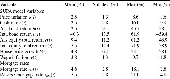

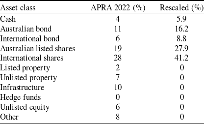
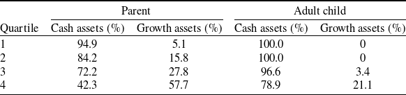
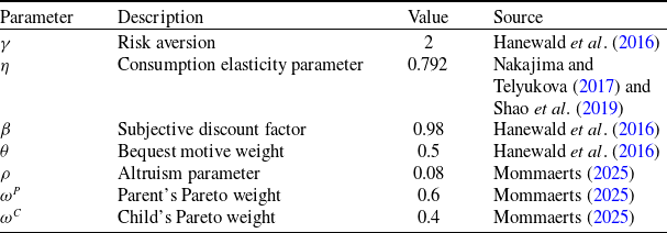

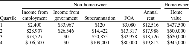
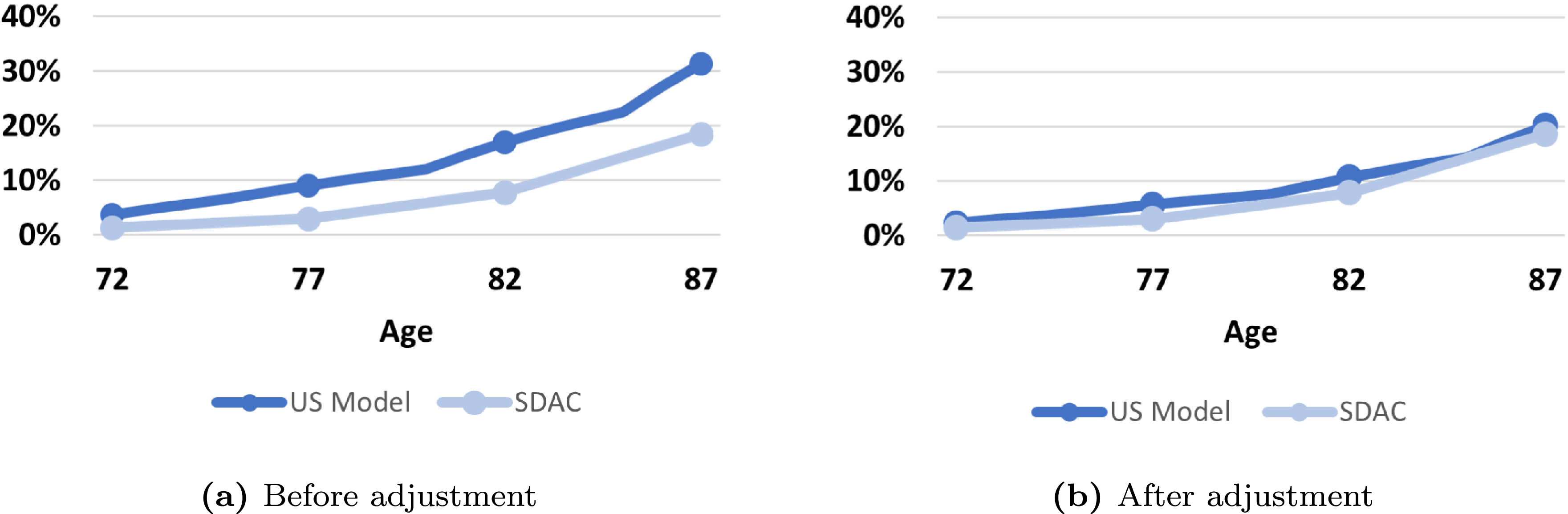
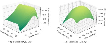
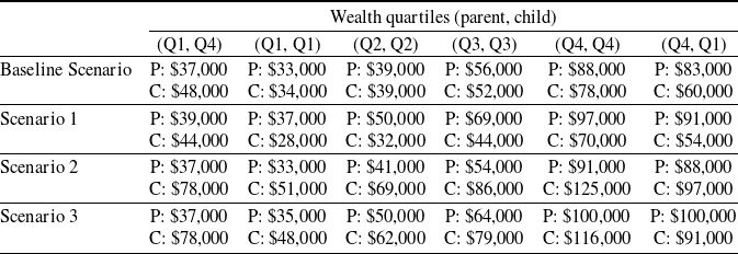
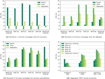
 ρ=0.08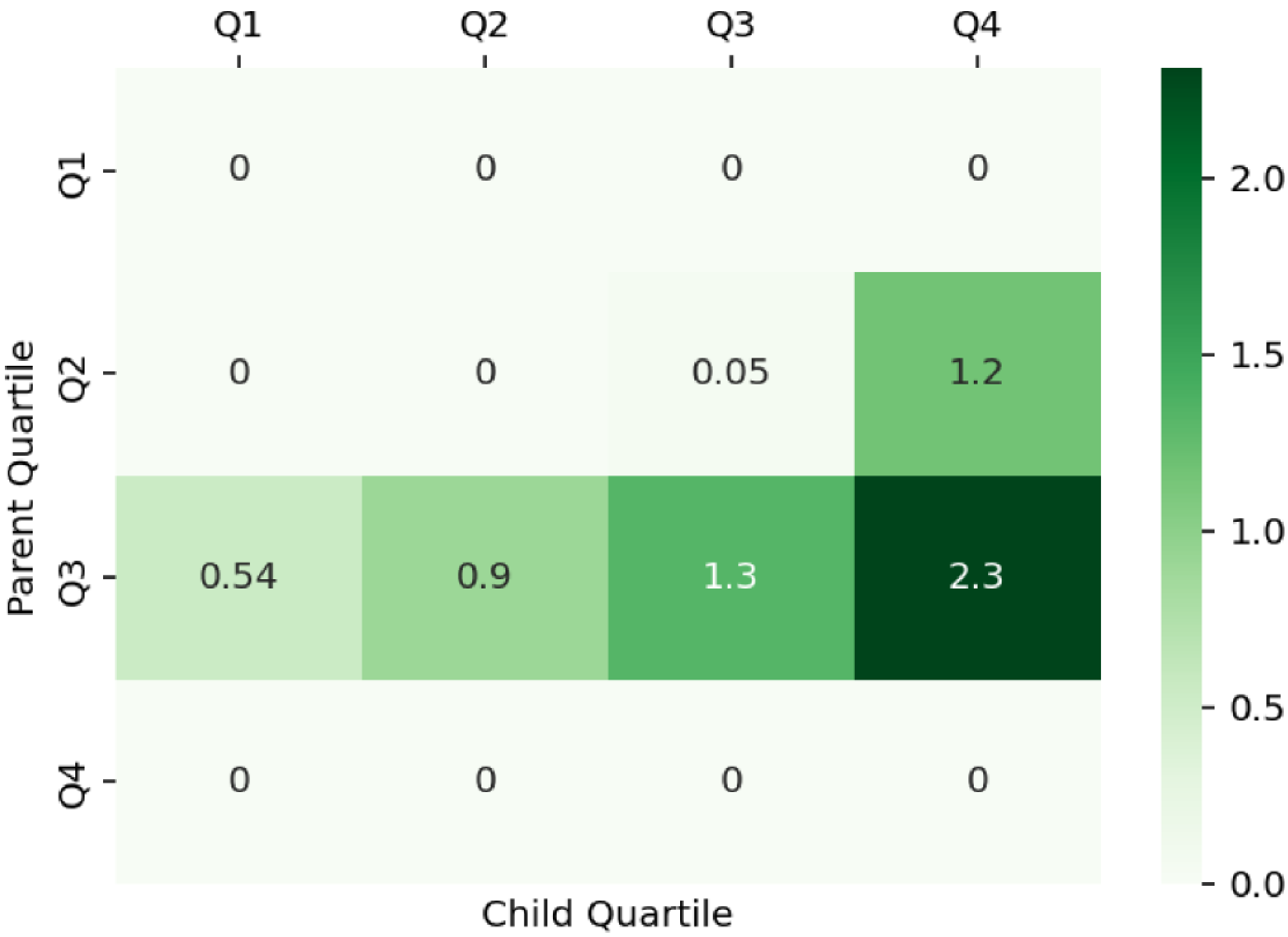
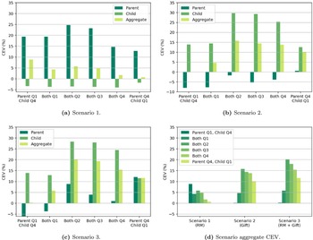
 ρ=0
ρ=0 ρ=0
ρ=0
 ρ
ρ ρ=0,0.001,0.08
 0.5
0.5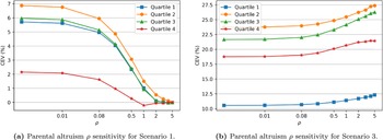
 ρ
ρ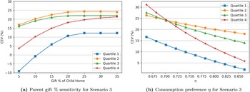
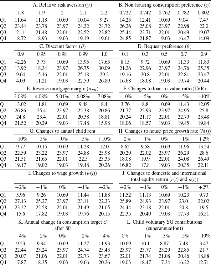


 Open access

