

1. Introduction
Structural changes in livestock markets, evolving marketing and pricing methods, thin markets, formula pricing, and price discovery have been at the center of much debate for decades. These concerns were a major catalyst to the passage of the Livestock Mandatory Reporting (LMR) Act of 1999 (Koontz and Ward, Reference Koontz and Ward2011). The LMR Act of 1999 mandated the secretary of agriculture to produce national cattle, beef, swine, sheep, and lamb price reports (U.S. Department of Agriculture, Agricultural Marketing Service [USDA-AMS], 2016). In 2012, the LMR Act of 1999 extended price reporting to include wholesale pork.
The hog market has experienced immense structural change since the LMR Act of 1999. Negotiated hog purchases went from representing more than 80% of daily hog slaughter volume in 1993 (Franken and Parcell, Reference Franken and Parcell2012; Lawrence, Reference Lawrence2010) to as little as 3% by 2013. Despite the marked decline in negotiated hog purchase volume, a significant share of market hogs are formula priced using thin reported negotiated market hog or wholesale pork prices as a base price in formulas (Lawrence, Reference Lawrence2010; Plain, Reference Plain2015). With such a thin market as is present for negotiated market hogs, the properties of transactions making up prices reported by the USDA-AMS are a concern. The purpose of this study is to determine the distributions of associated transactions that comprise the negotiated daily weighted-average USDA-AMS hog price report and the sensitivity of reported market hog prices to which plants purchase hogs each day.
Reductions in hog spot market participation caused by increased production contracts has raised concerns about price manipulation and helped to spur legislation requiring price reporting by packers (Key, Reference Key2010). Thinning spot markets reduces public market information and inhibits price discovery, which is a concern cited by pork producers (Key, Reference Key2010). The pork industry has considered base price alternatives along with policy changes for what information is reported within the LMR Act of 1999. Understanding current data limitations is important to assessing whether changes in negotiated price data collection will address underlying concerns with the negotiated spot market price data.
In accordance with the LMR Act of 1999, all federally inspected pork plants that process more than 100,000 head of hogs annually are mandated to daily report prices, volumes, and terms of transaction details to USDA-AMS (Franken, Parcell, Tonsor, Reference Franken, Parcell and Tonsor2011). One market report, of several that USDA-AMS summarizes and releases regarding hog price information, is the Daily Direct Prior Day – Purchased Swine (LM_HG200) report. The prior-day purchased report includes all transactions for hogs purchased in the negotiated market during the previous day. Transactions that comprise this report are analyzed in this study. The two main prices contained in this report are (1) the carcass-weight negotiated weighted-average base price and (2) the live-weight negotiated weighted-average price. Negotiated prices refer generally to bid-ask transactions between producer-sellers and packer-buyers. Negotiation here refers only to the base price and not negotiation of any merit-based adjustments to the base price. The negotiated carcass-weight price includes hogs that are marketed by producers to packers where the price is the negotiated base price for the hogs quoted on a carcass-weight basis. Hogs delivered on a carcass-weight negotiated base price may receive a different net price when they are delivered to the packer depending on the packer premium and discount schedule and carcass quality.Footnote 1 Live-weight negotiated hogs are bought by the packer on a live-animal weight basis, and no further price adjustment to the live price would generally occur when the hogs are delivered. The total number of hogs traded, volume-weighted-average prices, and the range of prices are reported for each of these two series in the USDA daily market reports.Footnote 2
As the negotiated live and carcass markets have become more thinly traded, questions have arisen regarding variation in the negotiated prices. Questions regarding the influence of individual packing plants on reported prices, the nature of the distribution of transactions that comprise price report summaries, and whether changes in reported prices from day to day reflect changing market fundamentals or nuances of which packers are participating in the market each day are immensely important in assessing the viability of USDA-AMS reported hog market prices.
Results from this study are important on several fronts. First, if reported prices are sensitive to which plants are buying hogs on any given day, prices may meander from day to day not necessarily because of fundamental changes in supply or demand, but because of which plants bought negotiated hogs. For those using USDA-AMS price reports for market information, the reported price change from one day to the next may not be a reliable indicator of evolving market conditions. Also, firms using the USDA-AMS reported prices in formula pricing agreements should be aware of reported price sensitivity for base prices. The USDA-AMS has considered reporting information that would illustrate variability present across individual transactions comprising the daily negotiated weighted-average reported prices beyond just the highest and lowest prices paid. However, to report a meaningful price variation metric, the distribution of the transactions comprising the weighted-average reported price must be known. For example, if transaction prices are normally distributed, reporting a standard deviation would suffice. However, if the transaction prices are not normally distributed, reporting a standard deviation could actually be misleading in that users would naturally infer price distributions from the standard deviation that would be incorrect. This study is designed to assess these important questions.
2. Past Literature
Several studies have explored dispersion in agricultural commodity prices. However, little has been done exploring price dispersion in reported hog market prices. Vukina and Zheng (Reference Vukina and Zheng2010) studied price dispersion in the hog market using individual transaction data in Iowa. Major packers’ individual procurement records in Iowa were obtained for the period October 8, 2002, to March 31, 2005. The original data contained 76,850 individual transactions of 4.8 million hogs. After screening data to meet USDA-AMS price reporting standards and removing transactions with less than five head, the data comprised 51,627 transactions containing 3.5 million hogs. Vukina and Zheng (Reference Vukina and Zheng2010) found that a large degree of intraday price dispersion was consistently present with an average price range around $15/hundredweight (cwt.) on any given day. The weighted-average daily price range represented approximately 25% of the mean transaction price. The authors formulated three hypotheses to explain price dispersion including farmer search cost, bargaining party patience, and asymmetric information. Regression analysis found evidence supporting all three hypotheses. Increasing lot size by one hog increased the price the farmer received by 1 cent/cwt. This is expected because packers gain cost efficiency by purchasing a larger volume of hogs from a single source in a single transaction. The authors concluded that farmers who had more information about the market while bargaining received higher prices for their hogs than farmers who were less informed. A producer who conducted business with one extra packer increased the base price received by 43 cents/cwt. The percentage of hogs secured through alternative marketing arrangements was negatively correlated with spot market prices.
Kim and Zheng (Reference Kim and Zheng2015) evaluated the impact on spot (negotiated) price volatility from changes in live-hog alternative marketing agreements. Using the USDA-AMS “National Daily Direct Hog Prior Day – Slaughter Swine” data series between January 2002 and December 2010 and a generalized autoregressive conditional heteroskedasticity–mean econometric model the authors determined that an increase in swine alternative marketing agreements increased spot price volatility and decreased spot price level. Short-run effects were small, but long-run effects more substantial. The authors suggest that their results may reveal increased packer market power because of an increase in alternative marketing agreements. The authors acknowledge that if hog quality is lower with spot price transactions, then their finding of a long-term lower spot price because of alternative marketing agreements is less worrisome. Finally, they determined that the long-term increase in alternative marketing agreements led to an increase in spot market price volatility.
Lawrence (Reference Lawrence1996) used killsheet data from specific hog producers in Iowa and found that prices across packers varied by as much as $1.84/cwt. after adjusting for back fat, yield, sort loss, and number of head per transaction. The economically most important price differentials across transactions were associated with variation in back fat, yield, and sort loss. Quality and quantity of hogs across locations have led to preferential pricing by some packers. Origin of livestock and regional packer concentration can also influence prices paid (Ward, Reference Ward2008).
Packers have been shown to pay lower prices for livestock (fed cattle) in concentrated regional markets during cooperative phases and purchase more aggressively during noncooperative conditions (Koontz, Garcia, and Hudson, Reference Koontz, Garcia and Hudson1993). Bailey and Brorsen (Reference Bailey and Brorsen1985) investigated the dynamic relationship between four regional cash prices for fed cattle using time series analysis and casualty tests. They found that regional meatpacker concentration may have reduced individual meatpacker market power in a given region because of local competition for limited supplies of livestock. Schroeder and Goodwin (Reference Schroeder and Goodwin1990) estimated the intertemporal price relationships among 11 regional slaughter cattle markets. Large-volume markets located in the major cattle feeding regions were dominant price discovery locations.
Market integration can also increase market power exercised by packers. Because a large percentage of hogs acquired by packers are under production contracts, this may influence packer market power in the spot market. Under production contracts, packers specify the quantity and quality before production occurs. Key (Reference Key2010) checked for evidence of market manipulation in the hog market by testing whether local prevalence of production contracts was correlated with spot market prices received by independent producers. He concluded that there was not an economically significant negative relationship between the share of local production delivered under contracts and the price received by independent producers.
3. Data
All individual transactions for carcass and live-hog negotiated purchases that are used to calculate the weighted-average prices that the USDA-AMS reports in the prior day purchased report (USDA, LM_HG200) over the period June 6, 2011, through December 17, 2013, were utilized for this study. The data include date, negotiated price, the packing plant and firm that bought the lot, the number of head included in the individual transaction, and whether the purchase was on a live- or carcass-weight basis. For live purchases, the estimated average live weight of hogs in the transaction was also collected by the USDA-AMS.
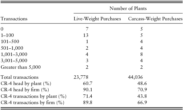
To be consistent with the transactions the USDA-AMS used to calculate weighted averages, they report in their daily market news that any transactions with an estimated average live-hog weight less than 240 lb. or greater than 300 lb. were dropped.Footnote 3 In addition, transactions that involved less than 10 head for live-hog negotiated transactions (consistent with filters the USDA-AMS uses) were deleted. After these filters were applied, a total of 67,814 negotiated transactions with 23,778 live- and 44,036 carcass-weight transactions (representing more than 10 million hogs) remained for analysis (Table 1).
Summary Statistics of Transactions Data
a HHI is the Herfindahl index: the sum of the squared market shares of all buyers each day in the respective live or carcass negotiated hog markets.
A combined 32 different packing plants purchased at least one lot of hogs in the negotiated live or carcass market during the time period. For each day, we calculated a plant Herfindahl index (HHI) to measure changes in buyer concentration across days. The average HHI was 0.18 for live-weight and 0.12 for carcass-weight purchases (Table 1). The HHIs did not have discernable trends over the time period, though the indexes varied noticeably across days. For example, the live-hog purchase HHI often varied from 0.10 to 0.30 in short time periods. The carcass purchase HHI was generally smaller than the live purchase HHI, and the carcass purchase HHI varied generally between 0.07 and 0.15.
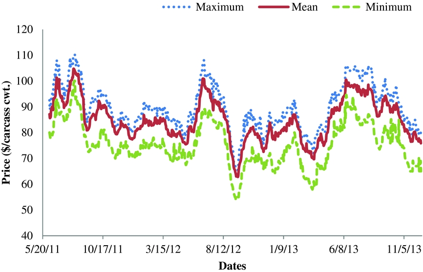
The weighted averages and daily ranges in the USDA-reported prices are illustrated in Figures 1 and 2 for negotiated live- and carcass-weight hog purchases, respectively. The range in live-hog negotiated prices exceeded 10% of the reported weighted-average price for 95% of the days, and the range exceeded 20% of the weighted-average during 16% of days. The carcass-weight negotiated base price ranges show similar variation with 98% of days having a range of 10% or more and 17% of days having a range of 20% or more of the weighted average. Both negotiated live and carcass weighted-average prices typically are closer to the maximum than the minimum price. For example, the negotiated live-hog purchase average low price was $8.05/cwt. less, and the average high price was $2.66/cwt. greater than the mean weighted-average price.
Daily Minimum, Maximum, and Weighted-Average Negotiated Live-Weight Hog Purchases

Daily Minimum, Maximum, and Weighted-Average Negotiated Carcass-Weight Hog Purchases
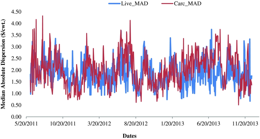
Daily transactions comprising the weighted-average prices were tested each day for normality, and normality was generally rejected (reported in detail in Section 5). Figure 3 illustrates the median absolute deviation (MAD) (because the daily prices were not normally distributed, average variation around the median is more meaningful than around the mean). Both live and carcass purchases exhibit similar variability. The average dispersion about the median was around $1/cwt. on some days and approached $4/cwt. on other days.
Daily Median Absolute Deviation for Live- and Carcass-Weight Hog Negotiated Purchases
Excluding weekends and holidays, there were 643 trading days (134 weeks) between June 6, 2011, and December 17, 2013. Not all plants made negotiated purchases during each trading day. Table 2 summarizes the number of days over the time period that plants made purchases. Only 9 of the 25 plants that made live-weight purchases bought hogs on more than half of the trading days, and only 5 participated in this market more than 75% of the days. This, together with the HHI, indicates that the live-weight negotiated market was oftentimes represented by a small number of plants that purchase hogs. The carcass-weight market had more plants (12 of 27) purchasing on at least 75% of the trading days.
Distribution of Plants by Number of Days out of 643 Total Trading Days Plants Had Negotiated Hog PurchasesFootnote a
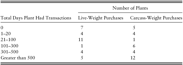
a Thirty-two plants total.
Table 3 provides a summary of the number of transactions represented by the 32 plants over the 643 trading days. Five plants had more than 3,000 transactions for live-weight purchases, and 6 plants had more than 3,000 transactions for carcass-weight purchases. The four-firm concentration ratio (CR-4) for live-weight negotiated purchases was 60.7% by plant and 90.1% by firm during this time frame. The CR-4 for carcass-weight negotiated purchases was 48.6% by plant and 70.9% by firm.
Distribution of Plants by Total Number of Transactions in Live- and Carcass-Weight Negotiated Purchases
Note: CR-4, four-firm concentration ratio.
4. Methods
To accomplish the objectives of this study, several analyses were completed. First, we tested the daily transaction prices for normality. If the transaction prices are normally distributed, the USDA might consider reporting standard deviations to aid in interpretation of daily price dispersion beyond simply reporting the high and low prices. However, if transaction prices are not normally distributed, reporting standard deviations illustrating price dispersion would be of limited value as MAD would be more useful. We also compare daily transaction price distributions to weekly distributions. On a weekly basis, there may be sufficient transactions to result in normally distributed prices even if daily transaction prices are not normally distributed.
To determine the influence each plant had on the daily weighted-average prices reported by the USDA-AMS, we removed each plant from the transaction data set, one at a time with replacement, and recalculated the daily weighted-average live and carcass prices. When a plant was removed, the new weighted-average price was compared to the weighted average reported by USDA-AMS for that day. This analysis was conducted for both live-weight and carcass-weight transactions separately. We categorized the changes in the weighted-average price resulting from removing individual plants into two categories for each live- and dressed-hog price as follows: (1) those for which when removing a plant the weighted-average price for each live- and carcass-weight negotiated purchase declined by more than $1/cwt. and (2) those for which when removing a plant the price increased by more than $1/cwt.
To further determine the impact of individual plants on the weighted-average price, regression analysis was performed. Four regression models were estimated: two for live-weight hog purchases and two for carcass purchases with transaction prices as the dependent variables. Harvey's multiplicative heteroskedasticity model (Harvey, Reference Harvey1976) was used for the estimation of parameters that may influence transaction prices of hogs. Harvey's multiplicative heteroskedasticity model produces unbiased and efficient estimates of parameters with error terms that are independently distributed (Belasco et al., Reference Belasco, Taylor, Goodwin and Schroeder2009).
Two different model structures were utilized: (1) a model with daily dummy variables included to account for daily supply-and-demand-driven aggregate market price changes and (2) a model using the previous day's wholesale pork cutout price as a base reflecting aggregate supply and demand instead of using the daily dummy variables.Footnote 4 The previous day's pork cutout price was used to reduce potential simultaneity bias and because today's bid/ask price negotiation between producers and packers starts with yesterday's cutout price as an important component of market information.
The second model specification was employed for two reasons. First, it provides a robust check of the plant dummy variable coefficients that provide evidence of variation in prices paid across plants. Plant and daily dummy variable impacts could be difficult to separate out individually if a plant only bought hogs on a few days during the sample period (Table 2). If both model specifications have similar plant dummy variable coefficient estimates, this provides confidence that the estimates reflect individual plant differences in typical prices paid and not differences in market prices during days they made purchases. Second, the model specification using the pork cutout price enabled us to include a daily buyer concentration variable in the model to determine if market structure influenced prices. In the model with daily dummy variables, the buyer concentration variable, by construction, was perfectly collinear with the set of daily dummy variables.
The live-hog price (LP) for each transaction was regressed as the dependent variable on estimated live weight (LW) and live weight squared (LWSq), number of head in the lot (Hd), and head squared (HdSq). Live weight was included in the models in quadratic form because light-weight hogs may be discounted as heavier carcasses are desired by packers, but at some point, carcass size gets too large for the plant production line and produces larger wholesale products than desired, and these heavier-weight hogs are discounted. Individual plant (Plantp, p = 1 to 32) and date of transaction (TrDayt, t = 1 to 643) were included as dummy variables in the first model, and the previous day's wholesale pork cutout (PorkCutout) price was substituted for the transaction day dummy variables in the second model. The data set contained 32 plants and 643 trading days. Daily dummy variables were included to adjust for changing price levels associated with changes in aggregate market supply and demand over time in model 1, and in model 2, the previous day's pork cutout price was used for this adjustment. To avoid perfect collinearity, a randomly selected plant dummy variable (Plant1) and the first trading day dummy variable in the data set were dropped. The first model (with transaction subscript i omitted for convenience) is the following (e1 is an error term):
 $$\begin{equation*}
\begin{array}{@{}l@{}} {\rm{Model}}\; 1\!\!:LP = {\beta _1} + {\rm{ }}{\beta _2}LW + {\beta _3}LWSq + {\beta _4}Hd + {\beta _5}HdSq + {\beta _6}Plant2 + \ldots \\ \quad \quad \quad \quad \quad \quad\quad + {\beta _{36}}Plant32 + {\beta _{37}}TrDay2 + \ldots + {\beta _{678}}TrDay643 + e1. \end{array}
\end{equation*}$$
$$\begin{equation*}
\begin{array}{@{}l@{}} {\rm{Model}}\; 1\!\!:LP = {\beta _1} + {\rm{ }}{\beta _2}LW + {\beta _3}LWSq + {\beta _4}Hd + {\beta _5}HdSq + {\beta _6}Plant2 + \ldots \\ \quad \quad \quad \quad \quad \quad\quad + {\beta _{36}}Plant32 + {\beta _{37}}TrDay2 + \ldots + {\beta _{678}}TrDay643 + e1. \end{array}
\end{equation*}$$
The dependent (explanatory) variables are referred to as conditional estimators, and the output variance is referred to as conditional variance. We modeled our heteroskedastic regressions (all the regression models for both live and carcass) according to Harvey's maximum likelihood estimation method (Harvey, Reference Harvey1976). In accordance with Harvey's specification, model 1 can be summarized as follows:
 $$\begin{equation*}
{y_i} = x_i^{\prime}\beta + {\epsilon _{\rm{i}}}.
\end{equation*}$$
$$\begin{equation*}
{y_i} = x_i^{\prime}\beta + {\epsilon _{\rm{i}}}.
\end{equation*}$$
Heteroskedasticity is corrected by specifying conditional variance, and this conditional variance is unique for each observation, that is, ε i ~ N(0, σ2 i ), with
 $$\begin{equation*}
\sigma _i^2 = {\sigma ^2}exp\left( {{z_i}^{\prime}\alpha } \right),
\end{equation*}$$
$$\begin{equation*}
\sigma _i^2 = {\sigma ^2}exp\left( {{z_i}^{\prime}\alpha } \right),
\end{equation*}$$
where α contains parameter estimates for each explanatory variable that weigh each characteristic by its effect on the individual variance term, and zi is a p × 1 vector of observations on a set of variables that affect the variance (the variables are the same as the dependent variables but without the intercept).
The second model is identical to the first except that the trading day dummy variables are replaced with the previous day's pork cutout price, PorkCutout(t-1). The previous day's pork cutout price is used to reduce potential simultaneity bias. A binary variable (Cutoutdummy) is included in model 2 that is equal to 1 after January 7, 2013, because the pork cutout price changed from voluntary to mandatory reporting with mandatory reported prices available starting January 7, 2013. Mandatory reported pork prices were notably higher than voluntary reported prices, so we added the binary variable to account for this discrete shift. Also added to model 2 is the natural log of the HHI, ln(HHI), to assess whether buyer concentration is related to negotiated transaction prices.
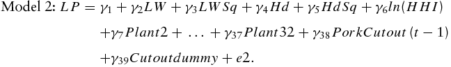 $$\begin{eqnarray*}
{\rm{Model}}\;2\!\!:LP &=& {\rm{ }}{\gamma _1} + {\rm{ }}{\gamma _2}LW{\rm{ }} + {\rm{ }}{\gamma _3}LWSq{\rm{ }} + {\rm{ }}{\gamma _4}Hd{\rm{ }} + {\rm{ }}{\gamma _5}HdSq{\rm{ }} + {\rm{ }}{\gamma _6}ln(HHI){\rm{ }}\\
&& + {\rm{ }}{\gamma _7}Plant2{\rm{ }} + {\rm{ }} \ldots {\rm{ }} + {\rm{ }}{\gamma _{37}}Plant32 + {\rm{ }}{\gamma _{38}}PorkCutout\left( {t - 1} \right){\rm{ }}\\
&& + {\rm{ }}{\gamma _{39}}Cutoutdummy{\rm{ }}+ {\rm{ }}e2.
\end{eqnarray*}$$
$$\begin{eqnarray*}
{\rm{Model}}\;2\!\!:LP &=& {\rm{ }}{\gamma _1} + {\rm{ }}{\gamma _2}LW{\rm{ }} + {\rm{ }}{\gamma _3}LWSq{\rm{ }} + {\rm{ }}{\gamma _4}Hd{\rm{ }} + {\rm{ }}{\gamma _5}HdSq{\rm{ }} + {\rm{ }}{\gamma _6}ln(HHI){\rm{ }}\\
&& + {\rm{ }}{\gamma _7}Plant2{\rm{ }} + {\rm{ }} \ldots {\rm{ }} + {\rm{ }}{\gamma _{37}}Plant32 + {\rm{ }}{\gamma _{38}}PorkCutout\left( {t - 1} \right){\rm{ }}\\
&& + {\rm{ }}{\gamma _{39}}Cutoutdummy{\rm{ }}+ {\rm{ }}e2.
\end{eqnarray*}$$
Similar models were also estimated using carcass prices (CP) as the dependent variables and dropping the weight variables from the right-hand side because these are not reported for carcass-weight purchases at the time the negotiation occurs. These models (estimated using Harvey's multiplicative heteroskedasticity model) were as follows:
 $$\begin{eqnarray*}
{\rm{Model}}\;3\!\!:CP &=& {\delta _1} + {\delta _2}Hd + {\delta _3}HdSq + {\delta _4}Plant2 + \ldots + {\delta _{34}}Plant32\\
&& + {\delta _{35}}TrDay2 + \ldots + {\delta _{676}}TrDay643{\rm{ }} + {\rm{ }}e3.
\end{eqnarray*}$$
$$\begin{eqnarray*}
{\rm{Model}}\;3\!\!:CP &=& {\delta _1} + {\delta _2}Hd + {\delta _3}HdSq + {\delta _4}Plant2 + \ldots + {\delta _{34}}Plant32\\
&& + {\delta _{35}}TrDay2 + \ldots + {\delta _{676}}TrDay643{\rm{ }} + {\rm{ }}e3.
\end{eqnarray*}$$
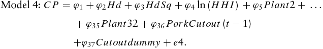 $$\begin{eqnarray*}
{\rm{Model}}\;4\!\!:CP{\rm{ }} &=& {\rm{ }}{\varphi _1} + {\rm{ }}{\varphi _2}Hd{\rm{ }} + {\rm{ }}{\varphi _3}HdSq{\rm{ }} + {\rm{ }}{\varphi _4}\ln \left( {HHI} \right){\rm{ }} + {\rm{ }}{\varphi _5}Plant2{\rm{ }} + {\rm{ }} \ldots\\
&& {\rm{ }} + {\rm{ }}{\varphi _{35}}Plant32 + {\rm{ }}{\varphi _{36}}PorkCutout{\rm{ }}\left( {t - 1} \right){\rm{ }}\\
&& + {\rm{ }}{\varphi _{37}}Cutoutdummy{\rm{ }} + {\rm{ }}e4.
\end{eqnarray*}$$
$$\begin{eqnarray*}
{\rm{Model}}\;4\!\!:CP{\rm{ }} &=& {\rm{ }}{\varphi _1} + {\rm{ }}{\varphi _2}Hd{\rm{ }} + {\rm{ }}{\varphi _3}HdSq{\rm{ }} + {\rm{ }}{\varphi _4}\ln \left( {HHI} \right){\rm{ }} + {\rm{ }}{\varphi _5}Plant2{\rm{ }} + {\rm{ }} \ldots\\
&& {\rm{ }} + {\rm{ }}{\varphi _{35}}Plant32 + {\rm{ }}{\varphi _{36}}PorkCutout{\rm{ }}\left( {t - 1} \right){\rm{ }}\\
&& + {\rm{ }}{\varphi _{37}}Cutoutdummy{\rm{ }} + {\rm{ }}e4.
\end{eqnarray*}$$
5. Results
The Shapiro-Wilk test was conducted on the daily transaction prices to test for normality.Footnote 5 The null hypothesis was that prices were normally distributed. As shown in Table 4, most of the daily transaction prices were not normally distributed. Only 14% (91 individual trading days) of the 643 trading days had transaction prices that were normally distributed at a 5% significance level for live-weight purchases, and less 1% of days were normally distributed for carcass-weight purchases. Because the assumption of normality was rejected in most of the daily transaction prices, weekly transaction data were also considered. Out of the 134 weeks of transactions, only 6 weeks (2.2%) satisfied the normality assumption at a 5% significance level for live purchases, and none did for carcass purchases. Kurtosis and skewness were also assessed. The nonparametric test of normality showed that live-hog and carcass daily transaction purchase prices for most days had high levels of skewness.
Normality Test on Daily and Weekly Live- and Carcass-Weight Negotiated Transactions

5.1. Plant Effects on Reported Prices
Table 5 summarizes the effect of each plant's purchases on reported weighted-average prices in live-hog and carcass purchases. Reported in the table is the count of the number of times each plant being included in the weighted-average price calculation either increased or reduced the weighted-average price by $1/cwt. or more grouped into 20-day categories. For example, 17 plants had between 1 and 20 days over the 643 trading days in which if they were not included in the weighted-average calculation, the market reported weighted-average live price declined by $1/cwt. or more. One plant had particularly noteworthy influence on live weighted-average prices with more than 61 days (nonconsecutive) out of the 643 trading days (exact number not reported because of confidentiality) in which when that plant purchased live hogs, their buying presence resulted in the reported weighted-average price being higher by at least $1/cwt. than it would have been had they not purchased hogs that day. Similarly, another plant had more than 61 trading days for which the weighted-average reported live-hog price was lower by $1/cwt. or more if their purchases were included in the weighted-average calculation.
Impacts of Individual Plants’ Purchases on Reported Live- and Carcass-Weight Negotiated Weighted-Average Price
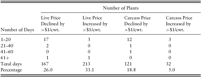
A total of 167 days of the 643 days (26%) had instances in which a particular plant not being included in the weighted-average calculation resulted in a decline in the live-hog weighted-average price (i.e., the market-reported weighted-average price was higher by more than $1/cwt. because of a plant's purchases being included in the weighted average), and for 213 days (33%), the reported weighted-average price was lower by more than $1/cwt. because of particular plant purchases. Combined, during 43% of days the calculated weighted-average live-hog price changed by a least $1/cwt. in absolute value (either up or down), and during 21% of days the carcass weighted-average price changed by at least $1/cwt. in absolute value. Overall, individual plants had much less frequent influence on the reported weighted-average carcass negotiated price than live purchases reflecting a thinner traded live market.
5.2. Transaction Price Regression Results
For the daily live-weight purchase regression models, 7 of the 32 plants were excluded. The excluded plants either did not report negotiated live-hog purchases or their purchases did not match average live-weight or number-of-head requirements for being included in the USDA-AMS report.
The variability in the daily weighted-average price can introduce excessive noise into the regression models, which leads to the presence of heteroskedasticity. Regression models were estimated using Harvey's heteroskedasticity specification. Harvey's multiplicative heteroskedasticity model provides unbiased and efficient estimates of the parameters. Harvey's parameter estimates have error terms that are identically and independently distributed.
The R-squared values for the live transaction models 1 and 2 were 0.91 and 0.72, respectively (Table 6). Head and head squared were statistically significant (0.05 level) in both models. Live weight and live weight squared were not statistically significant in model 1 but were in model 2. The pork cutout coefficient estimate of 0.68 indicated there was a $0.68/cwt. (live weight) increase in today's live-hog price for a $1/cwt. (carcass weight) increase in yesterday's pork cutout price. As expected, the Cutoutdummy variable coefficient was negative reflecting the increase in the reported pork cutout price that occurred after mandatory pork price reporting began.
Regression Results for Factors Explaining Individual Transaction PricesFootnote a
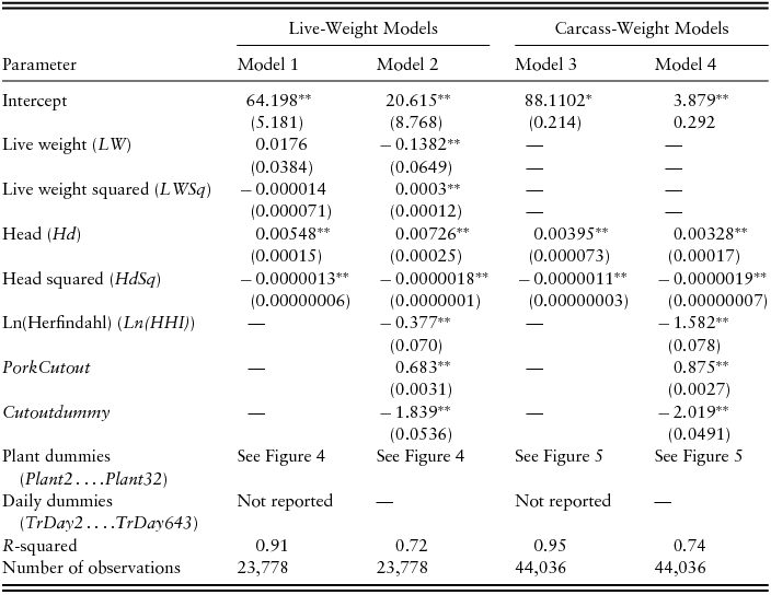
a Standard errors in parentheses.
Note: Asterisks (**) indicate statistically different from 0 at the 0.05 level.
Of most interest here are the plant dummy variable coefficients. The plant dummy variables capture spatial variation by accounting for localized supply and demand. The plant dummy variables also account for other nonmeasurable factors that could influence prices across plants. Such factors include transportation costs, plant-specific comparative advantages in processing or fabrication, and hog or carcass quality not captured in other variables in the model (i.e., plant-level premiums and discounts that yield a net price).Footnote 6
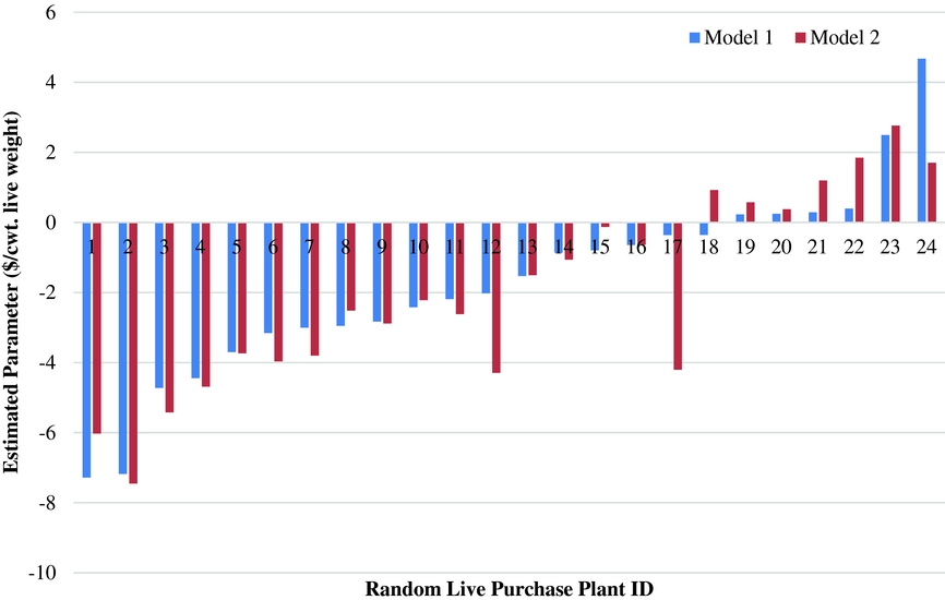
The plant dummy variable coefficients for live hogs were sorted from smallest to largest based on model 1 estimates and graphed to provide a visual summary of the estimates (Figure 4). As is evident, there was considerable variation in prices paid across plants. Twelve plants (model 1) and 13 plants (model 2) paid more than $2/cwt. less than the default plant. Four plants (model 1) and six plants (model 2) paid more than $4/cwt. less for live-hog purchases than the default plant. One plant paid more than $4/cwt. more than the default plant in model 1. Overall, the plant coefficients were similar across the two models with perhaps three exceptions (plants 12, 17, and 24) indicating that for the most part, the coefficient estimates were robust across the two model structures. The magnitude of differences in prices paid across plants indicates that which plants might be involved in trade in this thin market on any given day could have influenced prices reported in an economically important way. Because of confidentiality, we cannot discuss how plant location, size, or other plant or regional market characteristics might be associated with observed plant price differentials. The fact that the price differentials exist is sufficient for drawing important implications from this study.
Plant Binary Variable Parameter Estimates for Live-Weight Model 1 (daily dummies) and Model 2 (pork cutout)
The ln(HHI) variable was statistically significant at the 0.05 level. The coefficient estimate suggests that a 10% increase in HHI results in a $0.036/cwt. reduction in negotiated live transaction prices. A 90% interval around the average HHI (mean of HHI ± 1.65 times its standard deviation) was approximately 0.08 to 0.30 (Table 1), which corresponds with a $0.50/cwt. live-weight hog transaction price change interval (−0.377 × [ln(0.08) − ln(0.30)]). Overall, individual plant price differences were much larger than changes in daily price associated with changes in daily market participant concentration. This suggests that day-to-day prices varied more because of buying plants’ locations, local supply-and-demand conditions, and other plant-specific characteristics than overall buyer market concentration changes on any given day.
The conditional variance estimates for models 1 and 2 (results not tabulated) had several statistically significant coefficient estimates. Of most interest here is that more than half of the plant dummy variables were statistically significant relative to the base plant, suggesting that heteroscedasticity was related to plant purchase behavior.
In the carcass models 3 and 4, 5 of the 32 plants were not used in the regressions because no carcass hog transactions were recorded for them. The R-squared values for these models were 0.95 (model 3) and 0.74 (model 4). Again, head and head squared were statistically significant in these models. Also, the pork cutout (model 4) had a coefficient of 0.88, indicating that a $1/cwt. increase in yesterday's pork cutout price resulted in a $0.88/cwt. increase in today's negotiated hog carcass transaction price. Similar to the live model (model 2), the Cutoutdummy coefficient was statistically significant with a negative value as expected.
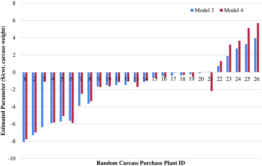
As with the live pricing models, the carcass pricing plant coefficients were sorted from smallest to largest and plotted for the two models to illustrate pricing variability across plants (Figure 5). Eight plants in each model paid at least $2/cwt. less than the default plant. Four plants (model 3) and three plants (model 4) paid more than $2/cwt. than the default. As with the live models, the plant coefficients were similar across the two models, with perhaps three or four exceptions (plants 3,Footnote 7 21, 25, and 26), again providing strong evidence that prices paid across plants vary in economically important ways.
Plant Binary Variable Parameter Estimates for Carcass-Weight Model 3 (daily dummies) and Model 4 (pork cutout)
For model 4, as buyer HHI increased by 10%, negotiated carcass hog prices declined by $0.15/cwt. carcass weight. Taking the mean HHI and adding and subtracting 1.65 times the standard deviation gives an HHI interval of 0.05 to 0.19, which corresponds to a price interval range of $2.11/cwt. carcass weight.
All the conditional variance estimates of the independent variables in model 3 were statistically significant at 0.05 level except three of the plant dummies. Approximately half of the plant dummy variables were statistically significant in the conditional variance model 4 as was ln(HHI). Overall, results of the conditional variance models indicate heteroscedasticity was conditional on plant purchase behavior in the carcass and the live markets.
6. Conclusion
Concerns about thin livestock markets have escalated as the percentage of animals represented in the price discovery process has trended downward to perilously low levels. In the hog market, negotiated daily price discovery represents less than 3% of producer-sold hogs on a typical day. One concern with such a thin market is that discovered and reported prices may not be representative of market supply-and-demand fundamentals. Furthermore, because reported negotiated prices are often used as base prices for formula pricing of hogs, this compounds potential concerns about thinly traded negotiated hog markets. This study focused on how thin hog markets affect reported prices published by the USDA-AMS. Individual transactions that the USDA-AMS used to compile daily live- and carcass-weight negotiated hog price reports reveal important implications about reported prices in this market.Footnote 8
Notable variation is present in transaction prices with a price range that exceeds 20% of the weighted-average reported price during 15% of days. With thin volume of trade, this raises concerns that small changes in volume on one side or the other of the median price could result in economically important movement in reported prices. The distribution of daily transaction prices tends to be negatively left skewed (toward lower prices), and the mean price is less than the median. As such, a small number of transactions take place at price levels much lower than the weighted-average associated with outlier trades or low-quality hogs. This is important information for anyone using the reported weighted-average prices as a base price to recognize because these low prices can have an economically important influence on the weighted-average reported price. Further, daily transaction prices are not normally distributed, so reporting information about the standard deviation of negotiated prices in daily negotiated hog market price reports is not meaningful.
With thin trade, a concern is that individual plants that purchase hogs on a particular day might influence reported prices. In a market with a large number of regularly participating buyers and large volume, individual buyers would not affect the weighted-average price. The negotiated hog market has notable spatial price variation, and most buyers do not participate most days in the negotiated hog market trade, making the number of buyers participating each day small. This results in individual plants buying hogs on a given day affecting reported prices at times by economically important amounts. For example, for 43% of the daily transactions analyzed, the reported live-hog market price would have been at least $1/cwt. higher or lower by eliminating individual plants from the weighted-average calculation. Clearly, individual plant participation in the negotiated hog market at times affects daily reported prices. Perhaps this is not surprising given the thinness of this market.
Overall, there are several implications of our results for industry participants. Current USDA-AMS reported daily negotiated hog prices are not necessarily a precise signal of evolving market conditions given the thinness of the market and frequency of influential plants on price. Price discovery in the negotiated market has economically important variation not necessarily completely associated with evolving market conditions from day to day. One of the more prominent sources of information relied on for price discovery is price information gleaned from recent transactions. However, relying on recent USDA-AMS weighted-average price quotes for current market information should be done with the recognition that the most recent quoted price is subject to which plants were actively buying during the time period of the price report. Variation in quoted prices from day to day occurs at times based on the set of plants that were engaged in the trade.
Producers and packers using reported negotiated daily prices as base prices in formula trades should be aware of the noise associated with reported prices and the associated sensitivity of reported prices to market participants. Because of this, we recommend exploring other options for base prices for formula trade than the thinly traded negotiated hog or carcass markets.
The USDA cannot fix the thin negotiated hog market problem through modifying price reporting protocols. The USDA-AMS market reports simply summarize the market trade that has occurred. Problems associated with thin hog markets are attributable to changing market structure and evolving pricing practices that have been driven by clear economic incentives for both producers and packers to move away from daily negotiated trade. At some point, if industry participants lose faith in the efficiency of reported negotiated prices, they will presumably quit using them as base prices in formula trade. Regardless, the best the USDA can do is to provide producers with information they can use to assess the thinness of reported prices and associated variation in those prices. Because daily transaction prices are not normally distributed, we recommend that the USDA-AMS should report a MAD in addition to the current reported market information, rather than the standard deviation, to provide more appropriate information on variation in reported prices that is more informative than just the high and low prices. The mean and standard deviation are strongly affected by outliers, and interpretation assumes that the distribution is normal. MAD is a more robust dispersion/scale measure in the presence of outliers (Leys et al., Reference Leys, Ley, Klein, Bernard and Licata2013). Interquartile range is another dispersion scale that can be useful. Both MAD and interquartile range are robust estimates of scale (Mostellar and Tukey, Reference Mosteller and Tukey1977). However, in a thinly reported market, like hogs, interquartile ranges potentially breach confidentiality rules for price reporting, which is a problem avoided when reporting MAD.
This study raises the need for additional research. Perhaps most apparent is that more work is needed to provide insight and guidance on how the hog industry can most effectively and efficiently move away from using negotiated prices in formula trade. A host of issues are present here, and they have not been adequately assessed as much of the work that has been completed is outdated (Schroeder, Mintert, and Berg, Reference Schroeder, Mintert and Berg2004). The livestock industry could benefit from further analysis to explore new options for effective and efficient price discovery. Continuing to explore useful market information that public agencies can collect and report to facilitate trade is another rich area for future work. The economic incentives that have led to thin negotiated livestock markets are strong, and moving back to more daily negotiation would be a costly undertaking. How the USDA can provide additional market information that can increase market efficiency under less daily negotiation is worth exploring.


 Open access