2 Empirical setting and notation

Each individual is characterized by three variables: the outcome of interest (Y), the group to which they belong (X) and the neighborhood in which they live (N). To keep things simple, we focus on the case in which group membership and the outcome of interest are each binary: $X\in \{0,1\}$ and $Y\in \{0,1\}$ . The analysis extends naturally to settings in which there are more than two groups or in which the outcome is continuous, as we discuss in the Supplementary Material.

We are primarily interested in the mean values of Y by group

$$ \begin{align*}Y^x=\mathbb{E}[Y|X=x],\end{align*} $$

as well as the difference in group means

$$ \begin{align*}D=\mathbb{E}[Y|X=1]-\mathbb{E}[Y|X=0].\end{align*} $$

Following the presentation of our main results, we also consider the identification of these statistics for specific neighborhoods (see Section 6).

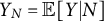
The core feature of the EI setting is that we do not observe individual-level values of X or Y. Rather, we observe one (aggregated) value of X and Y per neighborhood. We denote these aggregated values by $X_N=\mathbb {E}[X|N]$ and $Y_N=\mathbb {E}[Y|N]$ , respectively. We denote the neighborhood-level means of X and Y for a specific neighborhood n by $X_n=\mathbb {E}[X|N=n]$ and $Y_n=\mathbb {E}[Y|N=n]$ .

The distribution of individuals across neighborhoods is given by

$$ \begin{align*}P_n=\Pr(N=n).\end{align*} $$

We assume the researcher can directly observe $(X_n,Y_n,P_n)$ for each n, deferring issues of sampling uncertainty and statistical inference to our empirical application.

In our empirical application studying COVID-19 vaccinations, Y indicates whether an individual is vaccinated, X indicates whether an individual votes Republican and N indicates the county in which the individual resides. The share of vaccinated individuals in county n is denoted by $Y_n$ , and $X_n$ denotes the share of county residents who vote Republican. Our goal will be to use these county-level data to estimate the partisan vaccination gap, D, which we define as the difference in the mean vaccination rate of Republican relative to Democratic and third-party voters, $\mathbb {E}[Y\mid X=1]-\mathbb {E}[Y\mid X=0]$ .

Another common application of EI methods is to study group differences in voting behavior. For example, a researcher might seek to use precinct-level voting data to measure election turnout by race. In that setting, Y would indicate whether an individual votes, X would indicate membership in a particular racial group, and N would denote the individual’s precinct. The researcher would then infer differences in turnout rates by race (D) using the available precinct-level data on racial composition ( $X_N$ ) and turnout ( $Y_N$ ).

We next introduce a statistic summarizing the coarsening of the information on group membership (X) due to aggregation. By the law of total variance, we can decompose the total variation in X into the portions that are and are not explainable by neighborhood:Footnote ⁵

(1) $$ \begin{align} \operatorname{\mathrm{Var}}(X) = \operatorname{\mathrm{Var}}(X_N) + \mathbb{E}\left[\operatorname{\mathrm{Var}}(X) \mid N \right]. \end{align} $$

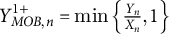
We then define the group aggregation ratio

$$ \begin{align*}\gamma=\frac{\operatorname{\mathrm{Var}}(X_N)}{\operatorname{\mathrm{Var}}(X)}\end{align*} $$

to measure the share of the total variance in group membership that is attributable to neighborhood.Footnote ⁶ When neighborhoods do not differ much in group prevalence, $\operatorname {\mathrm {Var}}(X_N)$ —and therefore $\gamma $ —will be small. In the extreme, when $\gamma =0$ , group composition does not vary at all across neighborhoods. Conversely, larger values of $\gamma $ correspond to more information on group membership being preserved, with $\gamma =1$ corresponding to the extreme scenario in which each neighborhood is entirely homogeneous by group (i.e., all individuals within the neighborhood are of the same group).Footnote ⁷ Because the ER estimator, and the bounds that we derive based on it, are not defined when $\gamma =0$ , we assume throughout that $\gamma \in (0,1]$ .

Many of our subsequent results relate to two conditional associations summarizing the relationship between X, Y and N. We define the between-group association as

$$ \begin{align*} \delta_B = \mathbb{E}\left[\text{Cov} \left( Y , X \, | \,N \right) \right]. \end{align*} $$

Intuitively, the between-group association measures differences in the outcome between individuals of different groups who live in the same neighborhood as one another. It reflects the portion of the association between X and Y that is not explained by neighborhood. In the context of our empirical application, for example, $\delta _B$ captures average within-county differences in vaccination uptake between Republican and Democratic voters. Similarly, in a voting turnout application, $\delta _B$ would reflect average racial differences in turnout among individuals in the same precinct.

The second conditional association on which we focus is the within-group association

$$ \begin{align*} \delta_W = \mathbb{E}\left[\text{Cov} \left( Y,X_N \, | \,X \right) \right]. \end{align*} $$

The within-group association captures within-group differences in the outcome across neighborhoods with different group compositions. That is, it measures the portion of the association between X and Y that is attributable to neighborhoods, holding individual group membership constant. To illustrate, in our empirical application, $\delta _W$ captures differences in vaccination uptake among individuals who are registered for the same political party who live in neighborhoods with differing concentrations of Republican voters. It would tend to be negative if Republican voters living in mostly-Republican neighborhoods were vaccinated at lower rates than Republican voters living in mostly-Democratic neighborhoods, and similarly, if Democratic voters living in mostly-Republican neighborhoods were vaccinated at lower rates than Democratic voters living in mostly-Democratic neighborhoods. In the context of a voter turnout study, $\delta _W$ would reflect differences in turnout among individuals of the same racial group living in precincts with differing concentrations of minority residents. For example, it would be non-zero if both minority and non-minority residents tended to be less likely to turn out for an election when their precinct has a high fraction of minority residents.

In the next section, we study canonical approaches to EI estimation through the lens of the group aggregation ratio and these conditional associations.

3 Canonical EI estimators

This section focuses on three common approaches for studying group-level differences in EI settings: ER, the NM and the MOB.Footnote ⁸ We present these familiar estimators informally; the Supplementary Material contains additional detail. For ease of exposition, we initially focus on identifying the difference in group means (i.e., D), deferring consideration of the levels of the group means (i.e., $Y^0$ and $Y^1$ ) to Section 5.

3.1 Ecological regression

The most common approach to EI is ER (Goodman Reference Goodman1953). The ER estimate for the difference in group means is the coefficient for $X_N$ from the weighted neighborhood-level regression of $Y_N$ on $X_N$ , with weights based on neighborhood population ( $P_n$ ). In our empirical application, for example, ER involves regressing county-level vaccination rates on county-level Republican vote shares; the ER estimate for the partisan vaccination gap is the estimated slope from this regression.

We focus on the ER estimator’s asymptotic limit under an iid sampling processFootnote ⁹:

$$ \begin{align*} D_{ER} = \frac{\text{Cov}(Y_N,X_N)}{\operatorname{\mathrm{Var}}(X_N)}. \end{align*} $$

The following proposition relates the bias of ER to the within-group association.Footnote ¹⁰

Proposition 1 Bias of ER for difference in group means

$$ \begin{align*} D_{ER} - D= \frac{ \delta_W}{\operatorname{\mathrm{Var}}(X_N)}, \end{align*} $$

where $ \delta _W = \mathbb {E}\left [\text {Cov} \left ( Y,X_N \, | \,X \right ) \right ].$

The proof of Proposition 1, and all subsequent results, is provided in the Supplementary Material.

When $\delta _W$ is non-zero, ER is biased because differences in the prevalence of groups across neighborhoods are conflated by other neighborhood-level contextual effects (Ansolabehere and Rivers Reference Ansolabehere and Rivers1995; Goodman Reference Goodman1953). Proposition 1 provides a simple expression for how such contextual effects shape this bias.

Proposition 1 implies the following corollary.

Corollary 1 The ER estimand, $D_{ER}$ , is unbiased if and only if $\delta _W=0$ .

A related condition that is often discussed in the EI literature is the constancy model, under which each group’s outcomes are the same in each neighborhood, $Y^x_n=Y^x$ for all n and for each $x\in \{0,1\}$ . Although this condition implies $\delta _W=0$ , the converse is not true.

3.2 The neighborhood model

An alternative EI method for estimating group differences is the so-called NM (Freedman et al. Reference Freedman, Klein, Sacks, Smyth and Everett1991).Footnote ¹¹ To estimate D, the NM first constructs estimates of $Y^0$ and $Y^1$ . Each group-specific estimate is formed from the weighted average of the outcome across neighborhoods, with weights equal to the specified group’s prevalence in each neighborhood. In our empirical application, for example, the NM estimate for the Republican vaccination rate is the average of county-level vaccination rates, weighted by the prevalence of Republicans in each county. The NM estimate for D is then formed as the difference in the NM estimates for $Y^0$ and $Y^1$ .

As with ER, we will focus on the NM estimator’s asymptotic limit:

$$ \begin{align*} D_{NM} = \frac{\mathbb{E}[X_N\,Y_N]}{\mathbb{E}[X_N]} - \frac{\mathbb{E}\left[ (1-X_N)\,Y_N \right]}{\mathbb{E} \left[ 1-X_N \right]}. \end{align*} $$

The following proposition shows that the bias of the NM is determined by the between-group association.

Proposition 2 Bias of the NM estimator for the difference in group means

$$ \begin{align*} D_{NM} - D = \frac{-\delta_B}{\operatorname{\mathrm{Var}}(X)}, \end{align*} $$

where $\delta _B=\mathbb {E}\left [\operatorname {\mathrm {Cov}}(X,Y|N) \right ].$

Intuitively, $\delta _B$ measures how much groups differ within the same neighborhood. If $\delta _B>0$ , group 1 tends to have higher outcomes than group 0 within each neighborhood. In that case, the NM, which effectively averages neighborhood outcomes weighting by group presence, tends to understate the true difference in group means because it ignores that group 1 individuals are disproportionately in higher-outcome positions within each neighborhood. Conversely, when $\delta _B<0$ , the NM overstates the difference in group means because it ignores that group 1 individuals tend to have lower outcomes than group 0 individuals within the neighborhoods being averaged.

Proposition 2 also implies the following corollary.

Corollary 2 The NM estimand, $D_{NM}$ , is unbiased if and only if $\delta _B=0$ .

Freedman et al. (Reference Freedman, Klein, Sacks, Smyth and Everett1991) noted that the NM point-identifies $\mathbb {E}[Y\mid X,N=n]$ for a specific neighborhood n under the related condition that there is no systematic difference in the outcome between groups within that neighborhood, that is, $\mathbb {E}[Y|0,N=n]=\mathbb {E}[Y|1,N=n]$ . Because our focus is on group differences over the entire population (rather than for a specific neighborhood), Corollary 2 requires only that there be no within-neighborhood differences on average.

We are now in a position to highlight some connections between the ER and NM approaches. First, note that the two estimands follow a close mechanical relationship, mediated by the group aggregation ratio.Footnote ¹²

Lemma 1 Relationship between NM and ER

$$ \begin{align*} D_{NM} =\gamma \,D_{ER}, \end{align*} $$

where $\gamma =\frac {\operatorname {\mathrm {Var}}(X_N)}{\operatorname {\mathrm {Var}}(X)}$ .

Using Lemma 1, we can next derive the following identity.

Proposition 3 Relationship of conditional associations and group aggregation ratio

$$ \begin{align*} D \, (1-\gamma) = \frac{\delta_W + \delta_B}{\operatorname{\mathrm{Var}}(X)}. \end{align*} $$

Because $\delta _W$ and $\delta _B$ control the respective biases of the ER and NM estimators, Proposition 3 shows that the performance of these estimators is fundamentally linked and related to the amount of information lost due to aggregation (via $\gamma )$ . In particular, when group prevalence does not vary much by neighborhood (so that most of the variation in X is within rather than between neighborhoods), will be small, and the sum will be large relative to the actual difference in group means, D. Finally, in conjunction with Corollaries 1 and 2, Proposition 3 establishes that except in special cases (i.e., $\gamma =1$ or $D=0$ ), the assumptions justifying the ER and NM estimators are mutually exclusive.

3.3 Method of bounds

Whereas ER and the NM yield point estimates for D, an alternative approach is to calculate the most extreme values of D that are consistent with the observed data. In EI settings with binary Y, consistency with the data requires that, for each neighborhood n, (i) $Y_n^0\in [0,1]$ ; (ii) $Y_n^1\in [0,1]$ ; and (iii) $X_n\,Y_n^1 + (1-X_n)Y_n^0=Y_n$ , where $Y_n^x=\mathbb {E}[Y|N=n,X=x]$ . The MOB interval for the group means is defined by the minimum and maximum values that satisfy these constraints. The interval for the difference in group means is then derived by comparing the minimum and maximum values that each group mean can take on.

Proposition 4 MOB for difference in group means

Define the following parameters:

$$ \begin{align*} D_{MOB}^{+} &= \frac{\mathbb{E}[\min\left\{Y_N,X_N\right\}]-\mathbb{E}[X_N]\mathbb{E}[Y_N]}{\operatorname{\mathrm{Var}}(X)} \\ \text{ and } D_{MOB}^- &= \frac{\mathbb{E}[Y_N](1-\mathbb{E}[X_N]) -\mathbb{E}[\min \{ Y_N,\,1-X_N \}] }{\operatorname{\mathrm{Var}}(X)}. \end{align*} $$

It follows that

$$ \begin{align*} D\in \left[ D_{MOB}^- \,,\, D_{MOB}^+ \right]. \end{align*} $$

These bounds are sharp.

The insight underlying Proposition 4 is originally due to Duncan and Davis (Reference Duncan and Davis1953); it has been extended and formalized by Horowitz and Manski (Reference Horowitz and Manski1995), Cross and Manski (Reference Cross and Manski2002) and Cho and Manski (Reference Cho and Manski2008), who focus on neighborhood-level bounds. Proposition 4 provides a closed-form expression for the aggregation of those neighborhood-specific bounds to the population-level.

We next relate the MOB interval to the ER and NM point estimates. Beginning with the latter, note that the aggregate data can never rule out the possibility that outcomes are homogeneous within neighborhoods, that is, that $\delta _B=0$ . Hence, the NM estimate is guaranteed to fall within the MOB interval.

Corollary 3 $D_{NM}\in \left [D_{MOB}^{-},D_{MOB}^{+}\right ].$

In contrast, no such guarantee is available for $\delta _W$ ; as a result, the ER estimate may sometimes be infeasible. Comparing the MOB endpoints to the expression for $D_{ER}$ in Proposition 1 sheds light on when this occurs.

Corollary 4

$$ \begin{align*} D_{ER}> D_{MOB}^+ &\iff \delta_W > \gamma \, \operatorname{\mathrm{Var}}(X) \, \left( D_{MOB}^+ - D\right), \,\text{ and }\\ D_{ER} < D_{MOB}^- &\iff \delta_W < -\gamma \, \operatorname{\mathrm{Var}}(X) \, \left( D-D_{MOB}^+\right). \end{align*} $$

Corollary 4 shows that ER is more likely to yield an infeasible estimate when $\gamma $ is small. Intuitively, when neighborhoods barely differ in their group composition, ER infers the slope based on small variations in $X_N$ . Any residual correlation between $X_N$ and $Y_N$ (reflected by a non-zero $\delta _W$ ) is thus amplified, leading to extreme values of $D_{ER}$ .

Because the bounds in Proposition 4 are sharp, they highlight the limits of what can be learned from the data in EI settings without imposing additional assumptions. In particular, the following lemma shows that the aggregate data are more informative about D as neighborhoods are more (internally) homogeneous with respect to either group membership or outcome.

Lemma 2 Width of MOB interval

$$ \begin{align*} D_{MOB}^+-D_{MOB}^- = \frac{1}{\operatorname{\mathrm{Var}}(X)} \mathbb{E}\left[ \min\{ X_N, 1-X_N, Y_N, 1-Y_N\} \right]. \end{align*} $$

To illustrate, suppose that individuals are perfectly sorted across neighborhoods according to their group, that is, $X_n\in \{0,1\}$ for all n. In this case, Lemma 2 shows that the MOB interval collapses to a single point (i.e., D). Moreover, because this setting (i.e., homogeneity of groups within neighborhoods) corresponds to $\gamma =1$ , Lemma 1 implies that $D_{NM}=D_{ER}$ . Finally, because the MOB interval always contains $D_{NM}$ (Corollary 3), it must be the case that all three of the canonical EI approaches converge on the true value of D. We can therefore conclude that $\gamma =1$ implies $D_{ER}=D_{NM}=D_{MOB}^-=D_{MOB}^+=D.$

A different limiting case occurs when individuals are sorted across neighborhoods according to outcomes rather than groups, that is, $Y_n\in \{0,1\}$ for all n. Here too, Lemma 2 implies that the MOB interval collapses to a single point, which again must coincide with both D and $D_{NM}$ . However, unless neighborhoods also happen to be perfectly homogeneous with respect to group, we will not have $\gamma =1$ , so from Lemma 1, we know that $D_{ER}\neq D_{NM}=D$ . Hence, whereas selection of individuals into neighborhoods according to group membership guarantees unbiasedness for all three of the canonical approaches, selection into neighborhoods according to outcomes implies that only the NM and the MOB will be unbiased.

Beyond these limiting cases, the informativeness of the MOB bounds for D can be related to the degree of information about X and Y lost through aggregation, as illustrated by the following proposition.

Proposition 5 Maximum width of the MOB interval

The MOB width is bounded as follows:

$$ \begin{align*} 0 \leq D_{MOB}^{+}-D_{MOB}^{-} \leq 2 \min \left\{ 1- \gamma,\frac{\operatorname{\mathrm{Var}}(Y)}{\operatorname{\mathrm{Var}}(X)} \left(1-\frac{\operatorname{\mathrm{Var}}(Y_N)}{\operatorname{\mathrm{Var}}(Y)}\right)\right\}. \end{align*} $$

Proposition 5 provides an upper bound on the width of the MOB interval; the actual interval may be more informative in a particular application. Interestingly, the proposition shows that D can be recovered with relative precision when either $\ \gamma $ or $\frac {\operatorname {\mathrm {Var}}(Y_N)}{\operatorname {\mathrm {Var}}(Y)}$ is close to $1$ . This is because extreme values of $X_n$ and $Y_n$ can independently constrain the range of feasible group means for a given neighborhood. In contrast, when aggregation eliminates most of the information about both X and Y, then the bounds on D may be relatively wide.

4 Signing the conditional associations

In this section, we study how assumptions about the sign of the within- and between-group associations can aid with identification.

We begin with the within-group association. When $\delta _W\geq 0$ , we know from Proposition 1 that ER will overstate the true difference in group means, that is, $D_{ER}>D$ . We can tighten our preexisting bounds for D (i.e., the MOB interval) by intersecting it with this new one-sided bound on D to obtain

(2) $$ \begin{align} \delta_W\geq 0 \implies D\in\left[{D_{MOB}^{-}},\, \operatorname{\mathrm{Min}}\left\{{D_{MOB}^{+}},\,D_{ER}\right\}\right]. \end{align} $$

The direction of the ER bias is reversed when $\delta _W\leq 0$ :

(3) $$ \begin{align} \delta_W\leq0 \implies D\in\left[\operatorname{\mathrm{Max}}\left\{D_{MOB}^{-},\,D_{ER}\right\},\,D_{MOB}^{+} \right]. \end{align} $$

We can proceed analogously to derive bounds based on the sign of the between-group association using Proposition 2:

(4) $$ \begin{align} \delta_B\geq0 \implies D\in\left[D_{NM}\,,\,D_{MOB}^{+} \right] \end{align} $$

and

(5) $$ \begin{align} \delta_B\leq0 \implies D\in\left[D_{MOB}^{-}\,,\, D_{NM}\right]. \end{align} $$

Because the NM estimate is guaranteed to be within the MOB interval (Corollary 3), the bounds in (4) and (5) have a simpler form than those appearing in (2) and (3).

Just as knowledge of the sign of one conditional association can aid in identification, knowledge of the signs of both $\delta _W$ and $\delta _B$ can further narrow the feasible range of values that D can take on. For example, if $\delta _B$ and $\delta _W$ are both known to be positive, one can intersect the bounds in (2) and (4) to obtain:

(6) $$ \begin{align} \delta_W\geq 0 \, \text{ and } \,\delta_B\geq 0 \implies D\in\left[D_{NM},\, \operatorname{\mathrm{Min}}\left\{D_{MOB}^{+},\,D_{ER}\right\}\right]. \end{align} $$

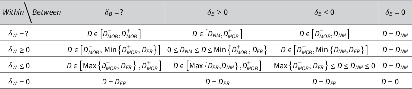
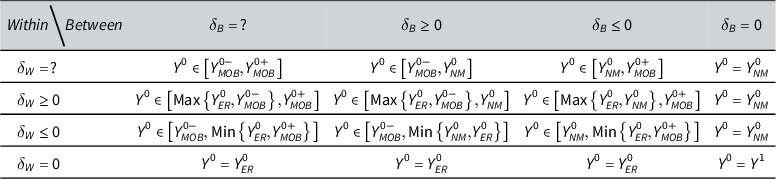
Table 1 applies the logic reflected in Equations (2)–(6) to describe what can be concluded about D based on what is assumed about $\delta _W$ and $\delta _B$ . When nothing is assumed (top-left cell), the identification region is equal to the MOB interval. At the other extreme, when either $\delta _W$ or $\delta _B$ is assumed to be zero (top row or rightmost column), the bounds reduce to either $D_{NM}$ or $D_{ER}$ .

Theorem 1 Identification of D with monotone EI

Suppose $\gamma \in (0,1)$ . Table 1 provides sharp bounds for D based on the specified assumptions.

Table 1

Identification of the difference in group means

Table 1 Long description

Starting from the top row, column headers are: Within / Between, delta sub B equals question mark, delta sub B greater than or equal to zero, delta sub B less than or equal to zero, delta sub B equals zero. The first column in each row shows the condition for delta sub W.For the first row, delta sub W equals question mark. From left to right, the entries in the first row are: D in left bracket D sub M O B superscript minus comma D sub M O B superscript plus right bracket; D in left bracket D sub N M comma D sub M O B superscript plus right bracket; D in left bracket D sub M O B superscript minus comma D sub N M right bracket; D equals D sub N M.For the second row, delta sub W greater than or equal to zero. From left to right, the entries in the second row are: D in left bracket D sub M O B superscript minus comma Min left bracket D sub M O B superscript plus comma D sub E R right bracket right bracket; zero less than or equal to D sub N M less than or equal to D less than or equal to Min left bracket D sub M O B superscript plus comma D sub E R right bracket; D in left bracket D sub M O B superscript minus comma Min left bracket D sub N M comma D sub E R right bracket right bracket; D equals D sub N M.For the third row, delta sub W less than or equal to zero. From left to right, the entries in the third row are: D in left bracket Max left bracket D sub M O B superscript minus comma D sub E R right bracket comma D sub M O B superscript plus right bracket; D in left bracket Max left bracket D sub E R comma D sub N M right bracket comma D sub M O B superscript plus right bracket; Max left bracket D sub M O B superscript minus comma D sub E R right bracket less than or equal to D less than or equal to D sub N M less than or equal to zero; D equals D sub N M.For the fourth row, delta sub W equals zero. From left to right, the entries in the fourth row are: D equals D sub E R; D equals D sub E R; D equals D sub E R; D equals zero.

Whereas the bounds in Equations (2)–(6) are based on assumptions about the respective signs of $\delta _W$ and $\delta _B$ , in some settings, it may be more credible to assume that $\delta _W$ and $\delta _B$ share the same sign as one another, without taking a stance on what that shared sign is. We refer to this condition, that is, that $\delta _B\cdot \delta _W \geq 0$ , as contextual reinforcement and illustrate the type of reasoning that might support it in Section 7.

Proposition 6 (Identification of group differences with contextual reinforcement)

If contextual reinforcement holds (i.e., if $\delta _W\cdot \delta _B\geq 0$ ), then either:

(i)

$$ \begin{align*} 0 \leq D_{NM} \leq D \leq \operatorname{\mathrm{Min}} \left\{D_{MOB}^{+}\,,\, D_{ER}\right\},\,\,\text{or} \end{align*} $$

(ii)

$$ \begin{align*} \operatorname{\mathrm{Max}} \left\{D_{MOB}^{-}\,,\, D_{ER}\right\} \leq D \leq D_{NM} \leq 0. \end{align*} $$

(iii) The bounds in (i) and (ii) are sharp.

The following corollary follows directly.

Corollary 5 If contextual reinforcement holds, then

$$ \begin{align*} \text{Sign}(D)=\text{Sign}\left( D_{ER} \right) = \text{Sign}\left( D_{NM}\right). \end{align*} $$

Thus, when contextual reinforcement holds, a researcher can look to the sign of $D_{NM}$ or $D_{ER}$ to learn which bounds apply, as well as to identify the sign of D.

Finally, like the MOB interval, the width of the contextual reinforcement bounds is shaped by $\gamma $ ; this is because $\gamma $ controls the divergence between $D_{NM}$ and $D_{ER}$ (see Lemma 1). Hence, when $\gamma $ is close to $1$ , $D_{ER}-D_{NM}$ will be small, and the contextual reinforcement bounds are guaranteed to be relatively informative about D.

5 Identification of group mean levels

This section maps our results for identifying the difference in group means, D, to the task of identifying the group means themselves, $Y^0$ and $Y^1$ . Each of the canonical EI approaches we have considered for estimating D can also be applied to estimate the levels of the group means.

With ER, this amounts to incorporating the estimated intercept term. Doing so yields the following estimands:

$$ \begin{align*} Y_{ER}^0 = \mathbb{E}[Y_N] - \left(\frac{\text{Cov}(Y_N,X_N)}{\text{Var}(X_N)}\right)\,\mathbb{E}[X_N] \end{align*} $$

and

$$ \begin{align*} Y_{ER}^1 = \mathbb{E}[Y_N] + \left(\frac{\text{Cov}(Y_N,X_N)}{\text{Var}(X_N)}\right)\,\left(1-\mathbb{E}[X_N]\right). \end{align*} $$

For the NM, the asymptotic limits of the group mean estimates are given by

$$ \begin{align*} Y^1_{NM} &= \frac{\mathbb{E}[X_N\,Y_N]}{\mathbb{E}[X_N]} \\[5pt] Y^0_{NM} &= \frac{\mathbb{E}\left[ (1-X_N)\,Y_N \right]}{\mathbb{E} \left[ 1-X_N \right]}. \end{align*} $$

Finally, for the MOB, intervals corresponding to the group mean levels are given by

$$ \begin{align*} Y^1 \in \left[ Y^{1-}_{MOB} \,,\, Y^{1+}_{MOB} \right] \end{align*} $$

and

$$ \begin{align*} Y^0 \in \left[ Y^{0-}_{MOB} \,,\, Y^{0+}_{MOB} \right], \end{align*} $$

where

$$ \begin{align*}Y_{MOB}^{1-} := \frac{\mathbb{E}[\max\left\{Y_N-(1-X_N),0 \right\}]}{\mathbb{E}[X]}\,\,,\,\,Y_{MOB}^{1+} := \frac{\mathbb{E}\left[\min\left\{Y_N,X_N\right\}\right\}]}{\mathbb{E}[X]}\end{align*} $$

and

$$ \begin{align*}Y_{MOB}^{0-} :=\frac{\mathbb{E}[\max\left\{Y_N-X_N,0\right\}]}{1-\mathbb{E}[X]} \,\,,\,\, Y_{MOB}^{0+} := \frac{\mathbb{E}[\min\left\{Y_N,1-X_N\right\}]}{1-\mathbb{E}[X]}.\end{align*} $$

We can relate the biases of the ER and NM estimates of $Y^0$ and $Y^1$ to $\delta _W$ and $\delta _B$ in a similar manner as we did for the corresponding estimators for D, as formalized in the following proposition.

Proposition 7 Bias of ER and NM for group means

$$ \begin{align*} Y^1_{ER} - Y^1= \frac{ \delta_W \, (1-\mathbb{E}[X])}{\operatorname{\mathrm{Var}}(X_N)}\,\,,\,\, Y^0_{ER} - Y^0= -\frac{ \delta_W \, \mathbb{E}[X]}{\operatorname{\mathrm{Var}}(X_N)} \end{align*} $$

$$ \begin{align*} Y^1_{NM} - Y^1= -\frac{ \delta_B}{\mathbb{E}[X]}\,\,,\,\, Y^0_{NM} - Y^0= \frac{ \delta_B}{1-\mathbb{E}[X]}. \end{align*} $$

We can now use the results in Proposition 7 to obtain bounds for the group means just as we used Propositions 1 and 2 to bound D in the prior section.

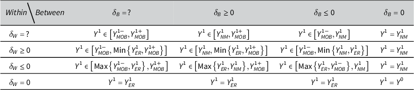
Theorem 2 Identification of Y with monotone EI

Suppose $\gamma \in (0,1)$ . Tables 2 and 3 provide sharp bounds for $Y^1$ (Table 2) and $Y^0$ (Table 3) under the specified assumptions.

Table 2

Identification of the group 1 mean

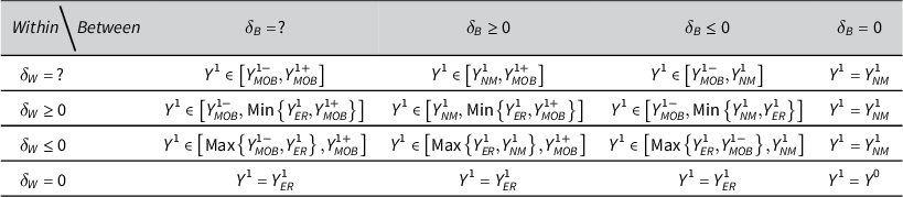
Table 2 Long description

Starting from the top row, column headers are: Within / Between, delta sub B equals question mark, delta sub B greater than or equal to zero, delta sub B less than or equal to zero, delta sub B equals zero. The first column in each row shows the condition for delta sub W.For the first row, delta sub W equals question mark. From left to right, the entries in the first row are: Y superscript 1 in left bracket Y sub M O B superscript 1 minus comma Y sub M O B superscript 1 plus right bracket; Y superscript 1 in left bracket Y sub N M superscript 1 comma Y sub M O B superscript 1 plus right bracket; Y superscript 1 in left bracket Y sub M O B superscript 1 minus comma Y sub N M superscript 1 right bracket; Y superscript 1 equals Y sub N M superscript 1.For the second row, delta sub W greater than or equal to zero. From left to right, the entries in the second row are: Y superscript 1 in left bracket Y sub M O B superscript 1 minus comma Min left bracket Y sub E R superscript 1 comma Y sub M O B superscript 1 plus right bracket right bracket; Y superscript 1 in left bracket Y sub N M superscript 1 comma Min left bracket Y sub E R superscript 1 comma Y sub M O B superscript 1 plus right bracket right bracket; Y superscript 1 in left bracket Y sub M O B superscript 1 minus comma Min left bracket Y sub N M superscript 1 comma Y sub E R superscript 1 right bracket right bracket; Y superscript 1 equals Y sub N M superscript 1.For the third row, delta sub W less than or equal to zero. From left to right, the entries in the third row are: Y superscript 1 in left bracket Max left bracket Y sub M O B superscript 1 minus comma Y sub E R superscript 1 right bracket comma Y sub M O B superscript 1 plus right bracket; Y superscript 1 in left bracket Max left bracket Y sub E R superscript 1 comma Y sub N M superscript 1 right bracket comma Y sub M O B superscript 1 plus right bracket; Y superscript 1 in left bracket Max left bracket Y sub E R superscript 1 comma Y sub M O B superscript 1 minus right bracket comma Y sub N M superscript 1 right bracket; Y superscript 1 equals Y sub N M superscript 1.For the fourth row, delta sub W equals zero. From left to right, the entries in the fourth row are: Y superscript 1 equals Y sub E R superscript 1; Y superscript 1 equals Y sub E R superscript 1; Y superscript 1 equals Y sub E R superscript 1; Y superscript 1 equals Y superscript 0.

Table 3

Identification of the group 0 mean

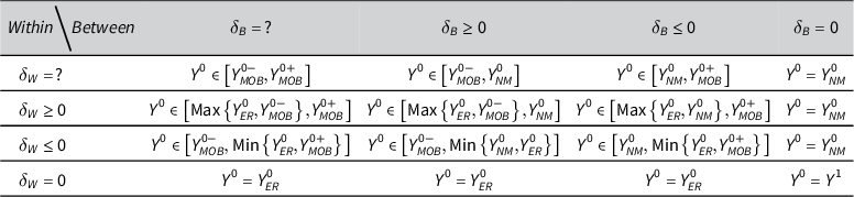
Table 3 Long description

Starting from the top row, column headers are: Within / Between, delta sub B equals question mark, delta sub B greater than or equal to zero, delta sub B less than or equal to zero, delta sub B equals zero. The first column in each row shows the condition for delta sub W.For the first row, delta sub W equals question mark. From left to right, the entries in the first row are: Y superscript 0 in left bracket Y sub M O B superscript 0 minus comma Y sub M O B superscript 0 plus right bracket; Y superscript 0 in left bracket Y sub M O B superscript 0 minus comma Y sub N M superscript 0 right bracket; Y superscript 0 in left bracket Y sub N M superscript 0 comma Y sub M O B superscript 0 plus right bracket; Y superscript 0 equals Y sub N M superscript 0.For the second row, delta sub W greater than or equal to zero. From left to right, the entries in the second row are: Y superscript 0 in left bracket Max left bracket Y sub E R superscript 0 comma Y sub M O B superscript 0 minus right bracket comma Y sub M O B superscript 0 plus right bracket; Y superscript 0 in left bracket Max left bracket Y sub E R superscript 0 comma Y sub M O B superscript 0 minus right bracket comma Y sub N M superscript 0 right bracket; Y superscript 0 in left bracket Max left bracket Y sub E R superscript 0 comma Y sub N M superscript 0 right bracket comma Y sub M O B superscript 0 plus right bracket; Y superscript 0 equals Y sub N M superscript 0.For the third row, delta sub W less than or equal to zero. From left to right, the entries in the third row are: Y superscript 0 in left bracket Y sub M O B superscript 0 minus comma Min left bracket Y sub E R superscript 0 comma Y sub M O B superscript 0 plus right bracket right bracket; Y superscript 0 in left bracket Y sub M O B superscript 0 minus comma Min left bracket Y sub N M superscript 0 comma Y sub E R superscript 0 right bracket right bracket; Y superscript 0 in left bracket Y sub N M superscript 0 comma Min left bracket Y sub E R superscript 0 comma Y sub M O B superscript 0 plus right bracket right bracket; Y superscript 0 equals Y sub N M superscript 0.For the fourth row, delta sub W equals zero. From left to right, the entries in the fourth row are: Y superscript 0 equals Y sub E R superscript 0; Y superscript 0 equals Y sub E R superscript 0; Y superscript 0 equals Y sub E R superscript 0; Y superscript 0 equals Y superscript 1.

Finally, if contextual reinforcement is assumed, one can first use Proposition 6 to learn the (common) sign of $\delta _B$ and $\delta _W$ , and then use that information to determine the applicable bounds on $Y^0$ and $Y^1$ from Tables 2 and 3.

6 Neighborhood-specific group means and differences

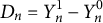
Our focus so far has been on group means for the overall population. In this section, we consider group means for individuals in a specific neighborhood, $Y_n^x=\mathbb {E}[Y\mid N=n,X=x]$ , or the difference in group means for individuals within that neighborhood, $D_n=Y_n^1-Y_n^0$ .

To start, recall that the MOB provides sharp bounds on $Y_n^x$ and $D_n$ for each n and x (Cho and Manski Reference Cho and Manski2008; Duncan and Davis Reference Duncan and Davis1953)Footnote ¹³:

$$ \begin{align*} Y_n^x \in \left[ Y_{MOB,n}^{x-} \,,\, Y_{MOB,n}^{x+} \right] \end{align*} $$

and

$$ \begin{align*} D_n \in \left[ D_{MOB,n}^{-} \,,\, D_{MOB,n}^{+} \right]. \end{align*} $$

As above, we can narrow the MOB interval by imposing sign restrictions on various aspects of the unobserved individual-level relationship between Y, X and N. Consider first the neighborhood-level analog to the between-group association, previously studied by Manski (Reference Manski2018). Define

$$ \begin{align*} \delta_{B,n}:= \operatorname{\mathrm{Cov}}(Y,X|N=n). \end{align*} $$

Whereas $\delta _B$ describes the average between-group variation within all neighborhoods, $\delta _{B,n}$ refers to the between-group variation for a specific neighborhood n. Because X is binary, $\delta _{B,n}=D_n\cdot \operatorname {\mathrm {Var}}(X|N=n)$ . It follows that

$$ \begin{align*}\delta_{B,n}\geq 0\iff \text{(i) } D_n\geq0 \text{, (ii) } Y_n^1\geq Y_n \text{ and (iii) } Y_n^0\leq Y_n.\end{align*} $$

As in Section 4, intersecting these one-sided bounds with the applicable MOB interval yields sharp bounds (Manski Reference Manski2018).

We next consider the identifying power of assumptions on the neighborhood-specific analog to the within-neighborhood association, which has not to our knowledge been studied in prior research. Let $\mu _x(x_n)$ denote the conditional expectation of Y for a member of group x in a neighborhood with group-prevalence $x_n$ :

$$ \begin{align*} \mu_{x}(x_n)= \mathbb{E}[Y \mid X=x,\,X_N=x_n]. \end{align*} $$

It will be convenient to assume that if two neighborhoods have the same group prevalence, they also share the same group meansFootnote ¹⁴:

$$ \begin{align*}Y^x_n=\mu_x(X_n) \,\text{ for all }x,n.\end{align*} $$

We also restrict our focus to neighborhoods with group prevalence values for which the first derivative of $\mu _x(\cdot )$ exists for each x, and we denote those derivatives by $\mu ^{\prime }_x(\cdot )$ .Footnote ¹⁵

For neighborhood n, define the local within-neighborhood association $\delta _{W,n}$ as

$$ \begin{align*} \delta_{W,n} = X_n \,\mu^{\prime}_1(X_n) + (1-X_n)\,\mu^{\prime}_0(X_n). \end{align*} $$

Conceptually, $\delta _{W,n}$ captures the within-group association between the mean of the outcome, Y, and the group prevalence of the neighborhood, $X_N$ , among individuals in neighborhoods with a particular level of group prevalence. It differs from $\delta _W$ in that $\delta _W$ depends on a summary measure of the relationship between Y and $X_N$ across all neighborhoods, whereas $\delta _{W,n}$ reflects the “local” relationship between Y and $X_N$ at a particular group prevalence level.

Although $\mu _0$ and $\mu _1$ are unobserved, we do observe the overall conditional expectation function of $Y_N$ given $X_N$ , which is the mixture of the group-specific conditional expectations functions

(7) $$ \begin{align} \mu(x_n) = x_n \,\mu_1(x_n) + (1-x_n) \, \mu_0(x_n). \end{align} $$

We also observe the derivative of the overall regression function, $\mu '(x_n)$ , which, by construction, is guaranteed to exist.

Differentiating (7) yields

(8) $$ \begin{align} \mu'(x_n) &=\mu_1(x_n) - \mu_0(x_n) + x_n \,\mu^{\prime}_1(x_n) + (1-x_n) \, \mu^{\prime}_0(x_n) \nonumber \\ &= D_n + \delta_{W,n}. \end{align} $$

Equation (8) links $D_n$ to the derivative of the conditional expectation function, which is observable, and to $\delta _{W,n}$ , which is not. An assumption about the sign of $\delta _{W,n}$ can therefore be combined with observation of $\mu '(X_n)$ to bound $D_n$ , and by extension, $Y_n^0$ and $Y_n^1$ , as formalized in the following proposition.

Proposition 8 (i) If $\delta _{W,n} \geq 0$ :

$$ \begin{align*} D_n &\in\left[ D_{MOB,n}^{-}, \min\left\{\mu'(X_n), D_{MOB,n}^+\right\}\right], \\ Y_n^1 &\in [Y_{MOB,n}^{1-}, \min \left\{Y_{MOB,n}^{1+}, Y_n + (1-X_n)\cdot \mu'(X_n)\right\}], \\ \text{ and } Y_n^0 &\in [\max\left\{Y_{MOB,n}^{0-}, Y_n-X_n\cdot \mu'(X_n)\right\}, Y_{MOB,n}^{0+}]. \end{align*} $$

(ii) If $\delta _{W,n}\leq 0$ :

$$ \begin{align*} D_{n} &\in \left[ \max\left\{\mu'(X_n),D_{MOB,n}^{-}\right\} , D_{MOB,n}^+ \right], \\ Y_n^1 &\in [\max\left\{Y_{MOB,n}^{1-},Y_n+(1-X_n) \cdot \mu'(X_n)\right\}, Y_{MOB,n}^{1+}], \\ \text{ and } Y_n^0 &\in [Y_{MOB,n}^{0-},\min\left\{Y_{MOB,n}^{0+},Y_n-X_n\cdot \mu'(X_n)\right\}]. \end{align*} $$

(iii) The bounds in (i) and (ii) are sharp.

Intuitively, the bounds in Proposition 8 are the neighborhood-specific analog to the population-level bounds based on the sign of $\delta _W$ that were derived in Sections 4 and 5. The main difference is that the neighborhood-specific version relies on the derivative of the conditional expectation function $\mu '(x_n)$ , which serves as a local version of the ER slope.

These bounds can be further narrowed by combining assumptions on the signs of the (local) conditional associations, as in the earlier sections.

Finally, consider the possibility that the researcher has information not about the individual signs of $\delta _{W,n}$ and $\delta _{B,n}$ but rather that these two (local) conditional associations share the same sign as one another. This is the local analog to contextual reinforcement and yields an analogous identification result.

Proposition 9 Suppose that $\delta _{B,n} \cdot \delta _{W,n}\geq 0$ . Then:

(i)  $\mu '(X_n)\geq 0$ implies

$$ \begin{align*} D_n &\in \left[ 0, \min\left\{\mu'(X_n),D_{MOB,n}^{+}\right\}\right], \\ Y_n^1 &\in \left[Y_n, \min\left\{Y_n + (1-X_n)\mu'(X_n), Y_{MOB}^{1+}\right\}\right], \\ \text{ and } Y_n^0 &\in \left[\max\left\{Y_{MOB,n}^{0-},Y_n- X_n \, \mu'(X_n) \right\}, Y_n \right]. \end{align*} $$

(ii)  $\mu '(X_n)\leq 0$ implies

$$ \begin{align*} D_n &\in [\max\left\{\mu'(X_n),D_{MOB,n}^-\right\},0], \\ Y_n^1 &\in [\max\left\{Y_{MOB,n}^{1-},Y_n+(1-X_n)\mu'(X_n)\right\},Y_n], \\ \text{ and } Y_n^0 &\in [Y_n,\min\left\{Y_n-X_n\mu'(X_n), Y_{MOB,n}^{0+}\right\}]. \end{align*} $$

(iii) The bounds in (i) and (ii) are sharp.

(iv)  $\text {Sign}(D_n)=\text {Sign}\left (\mu '(X_n)\right ).$

We will illustrate these bounds in our empirical application, described in the following section.

7 Empirical application

To illustrate an application of monotone EI, we investigate partisan polarization in COVID-19 vaccine uptake. This question has been of interest to policymakers, academics and the media (Collins Reference Collins2024; Jones and McDermott Reference Jones and McDermott2022; Milligan Reference Milligan2021). Most research in the U.S. context has had to rely on EI, as joint individual data on vaccination status and partisan membership are not available for a large nationally representative set of individuals (e.g., Albrecht Reference Albrecht2022; Ye Reference Ye2023).

Our primary dataset consists of county-level data from 3,115 counties on COVID-19 vaccination uptake and partisanship. We measure vaccination uptake as the share of county residents who had received one or more COVID-19 vaccinations as of December 31, 2021, obtained from the Centers for Disease Control and Prevention (2024). We measure partisanship as the fraction of voters in the county who cast their ballot for the Republican candidate in the 2020 presidential election, obtained from the MIT Election Data and Science Lab (2020).Footnote ¹⁶ Our goal is to use the county-level data to estimate the partisan vaccination gap, which we define as the difference in the mean vaccination rate of Republican voters relative to Democratic and third-party voters.

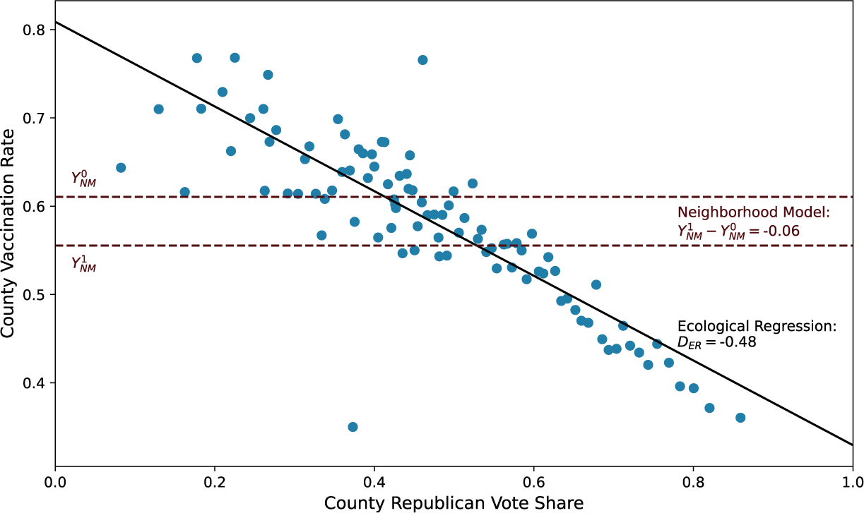
Figure 1 plots the binned county-level data. The figure shows a clear downward trend: counties with higher Republican vote share tend to have lower vaccination rates. The pattern is consistent with the possibility that Republican voters are vaccinated at lower rates than Democratic and third-party voters. However, this interpretation is potentially subject to the ecological fallacy; counties with higher Republican voter share may have lower vaccination rates for reasons unrelated to partisan composition (Ye Reference Ye2023). Indeed, the MOB interval for the partisan vaccination gap ranges from $-$ 77.4 to 52.8 percentage points. Without further assumptions, the county-level data do not provide much information about the magnitude or even direction of partisan differences in vaccinations. Point identification approaches also diverge sharply: the NM and ER imply respective partisan vaccination gaps of $-$ 5.5 and $-$ 47.9 percentage points.

Figure 1

County vaccination rate by county Republican vote share.

Note: The figure reports county-level COVID-19 vaccination rates by the share of voters in the county who voted for the Republican candidate in the 2020 presidential election. Counties are grouped into 100 equal-population bins. The neighborhood model estimates for the mean vaccination rates among Republican and non-Republican voters are, respectively, denoted by the lower and upper red dotted lines. The ecological regression line is in black.

Figure 1. Long description

The x-axis is labeled County Republican Vote Share, ranging from 0.0 on the left to 1.0 on the right. The y-axis is labeled County Vaccination Rate, ranging from 0.4 at the bottom to 0.8 at the top. Blue dots represent county-level data, distributed from the upper left to the lower right, indicating a negative trend. A solid black line runs diagonally downward, labeled Ecological Regression D sub E R equals negative 0.48, showing a strong negative linear relationship. Two horizontal red dotted lines are present: the upper line is labeled Y sub N M superscript 0, the lower line is labeled Y sub N M superscript 1. The difference between these lines is marked as Neighborhood Model Y sub N M superscript 1 minus Y sub N M superscript 0 equals negative 0.06. The red lines represent estimated mean vaccination rates for non-Republican and Republican voters, respectively. The black regression line shows the overall ecological association between Republican vote share and vaccination rate.

To sharpen identification through monotone EI, consider first the sign of the between-group association, $\mathbb {E}\left [\text {Cov}(Y,X|N)\right ]$ , which here refers to differences in vaccination uptake between Republican and Democratic voters living in the same county. Prior research provides some basis for expecting the between-group association to be negative; there are well-documented partisan differences in information sources that are not fully mediated through neighborhood (Iyengar and Hahn Reference Iyengar and Hahn2009; Peterson, Goel, and Iyengar Reference Peterson, Goel and Iyengar2021), and the prominent Republican politicians featured on more conservative media outlets were more likely to espouse anti-vaccination beliefs and/or downplay the health risks associated with the COVID-19 virus as vaccinations were made available (Albrecht Reference Albrecht2022; Gollwitzer et al. Reference Gollwitzer2020; Hornsey et al. Reference Hornsey, Finlayson, Chatwood and Begeny2020).

The within-group association, $\mathbb {E}\left [\text {Cov}(Y,X_N|X)\right ]$ , refers to differences in vaccination uptake among individuals who vote for the same political party who live in neighborhoods with differing concentrations of Republican voters. Like the between-group association, there is some reason to expect the within-group association to be negative. For example, Republican counties tend to be lower income and more rural (Figure S2 in the Supplementary Material), which are factors associated with lower access to public health services like vaccinations (Hernandez et al. Reference Hernandez, Dickson, Tang, Gabriel, Berenbrok and Guo2022; Parolin and Lee Reference Parolin and Lee2022; Sun and Monnat Reference Sun and Monnat2022).

More generally, there are reasons to expect that the two conditional associations share the same sign as one another, whether that sign is positive or negative. One mechanism through which such contextual reinforcement may operate is network effects, such as social norms or peer effects. In particular, people’s health behaviors are known to be influenced by the people around them (Klaesson, Lobo, and Mellander Reference Klaesson, Lobo and Mellander2023; Sato and Takasaki Reference Sato and Takasaki2019), and in mostly Republican counties, a larger share of the people with whom one interacts are likely to be Republican. Thus, if the Republicans in a neighborhood tend to be more skeptical of COVID-19 vaccinations (i.e., the between-group association is negative), that is likely to reduce the vaccination rate among both Democrats and Republicans living in that neighborhood. In the words of one author, “In many communities, wearing a mask or getting a [COVID-19] vaccine became a political statement, with many Republicans arguing that these actions violated their individual freedoms and were unnecessary anyway” (Albrecht Reference Albrecht2022). Along similar lines, for many people, vaccine uptake may depend in part on local policies, such as whether vaccines are mandated for public sector employees (Howard-Williams et al. Reference Howard-Williams, Soelaeman, Fischer, McCord, Davison and Dunphy2022). Thus, if Republicans exhibit more vaccine hesitancy, we would expect that counties in which more Republicans live would be more likely to elect leaders that do not adopt pro-vaccine policies, leading to lower vaccine rates for county residents, whether Democratic or Republican.Footnote ¹⁷

Figure 2

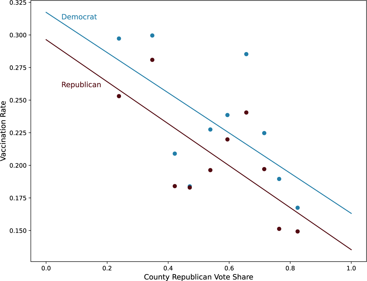
Vaccination rate by vote share and political party membership.

Note: The figure uses the matched auxiliary dataset to report COVID-19 vaccination rates by county-level Republican vote share for individuals registered as Republicans (red) and individuals registered as Democrats (blue). Individuals are grouped into ten equal-sized bins based on the Republican vote share for the county in which they live. The average vertical difference between the blue and red points reflects the estimated sign of $\delta _B$ . The average slope of the linear best fit lines reflects the estimated sign of $\delta _W$ .

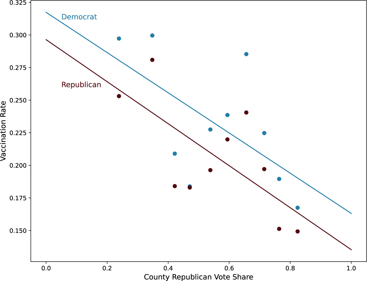
Figure 2. Long description

The scatter plot has the x-axis labeled County Republican Vote Share, ranging from 0 to 1, and the y-axis labeled Vaccination Rate, ranging from 0.15 to 0.325. Blue dots represent Democrats and red dots represent Republicans, each plotted in ten equal-sized bins based on the Republican vote share along the x-axis. For each bin, the blue dots are positioned above the red dots, indicating higher vaccination rates for Democrats at every level of Republican vote share. Both groups show a downward linear trend as Republican vote share increases. The blue trend line for Democrats starts near 0.32 on the y-axis at the left and slopes downward to about 0.19 at the right. The red trend line for Republicans starts near 0.28 on the y-axis at the left and slopes downward to about 0.15 at the right. The vertical gap between the two lines remains roughly constant across the x-axis.

The foregoing discussion provides a theoretical basis for the contextual reinforcement assumption in this setting. We empirically validate the assumption by drawing on an auxiliary dataset that contains individual-level data on vaccination status, political party registration and neighborhood.Footnote ¹⁸ We construct this dataset by matching a national dataset of voter registration records (L2 2024), which contains individual-level data on political party, to a large dataset of electronic health care records (Balraj et al. Reference Balraj, Vala, Hao, Philofsky, Tsvetkova, Trach, Narra, Zhuk, Shamkhorskaya, Singer, Mesterhazy, Datta, Chu and Rehkopf2023), which contains individual-level data on COVID-19 vaccination status. Appendix E of the Supplementary Material provides a further description of the underlying data sources and of our matching procedure. The final matched dataset contains approximately 1.3 million registered Republicans and Democrats in 2,576 counties and 49 states, plus the District of Columbia.Footnote ¹⁹

Figure 2 uses the auxiliary data to plot vaccination rates by (binned) county-level Republican vote share, separately for registered Republicans and Democrats. The figure provides visual support for contextual reinforcement: the Republican bins tend to lie below the Democratic bins with similar partisan makeup (so that the between-group association is negative) and both the Republican bins and Democratic bins exhibit a downward sloping trend (so that the within-group association is also negative). Formal statistical tests regarding the sign of these quantities yield the same conclusion (see Table S3 in the Supplementary Material). Based on these results, we adopt the contextual reinforcement assumption to interpret the county-level analyses.Footnote ²⁰

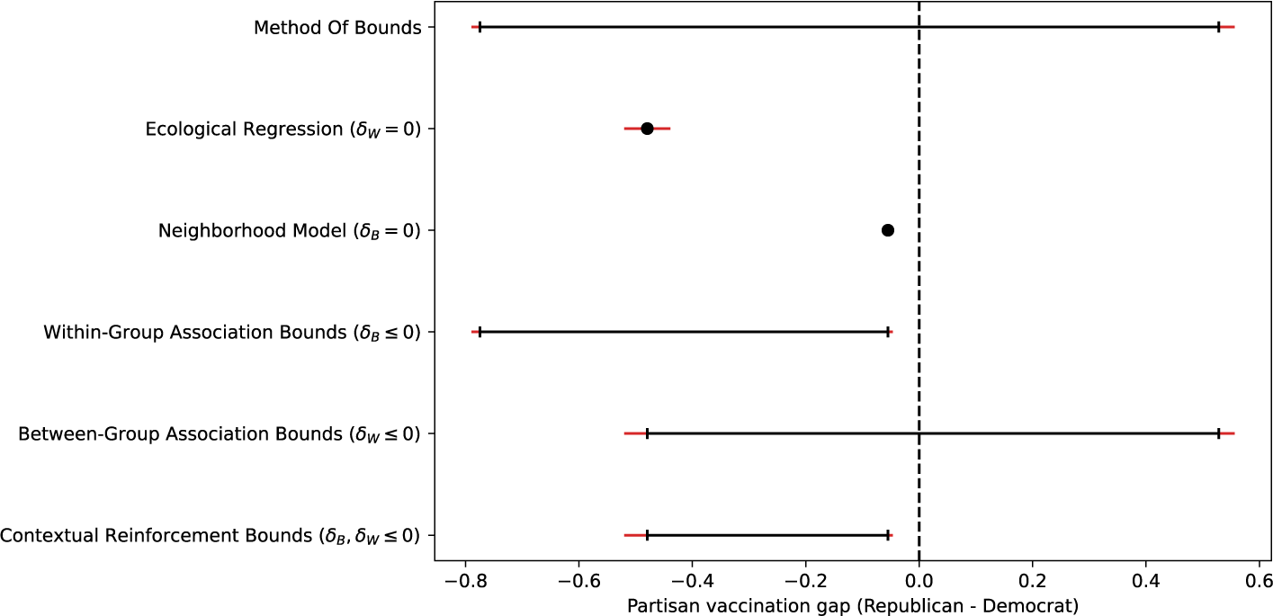
When contextual reinforcement holds, Corollary 5 establishes that we can identify the sign of the difference in group means based on the sign of the difference between the NM and ER estimators. As shown in Figure 3, we find that this difference is positive ( $p<0.01$ ), implying that Democrats are vaccinated at higher rates than Republicans. In turn, the contextual reinforcement bounds from Proposition 6 imply that the partisan vaccination gap is between $-$ 47.9 and $-$ 5.5 percentage points (95% CI: $-$ 51.8 to $-$ 5.1).

Figure 3

Identification of partisan vaccination gap using monotone EI.

Note: The partisan vaccination gap is defined as the proportion of vaccinated Democratic voters (and third-party supporters) subtracted from the proportion of vaccinated Republican voters. A negative gap indicates that a lower share of Republican voters are vaccinated. Red bars are 95% confidence intervals following Imbens and Manski (Reference Imbens and Manski2004); the confidence intervals are based on standard errors from a county-level bootstrap with 1,000 bootstrap replicates.

Figure 3. Long description

The x-axis is labeled Partisan vaccination gap (Republican minus Democrat) and ranges from negative zero point eight to zero point six. The y-axis lists six methods from top to bottom: Method Of Bounds, Ecological Regression (delta sub W equals zero), Neighborhood Model (delta sub B equals zero), Within-Group Association Bounds (delta sub B less than or equal to zero), Between-Group Association Bounds (delta sub W less than or equal to zero), and Contextual Reinforcement Bounds (delta sub B, delta sub W less than or equal to zero). Each method is represented by a black dot for the point estimate and a horizontal black line with red end caps for the ninety-five percent confidence interval. All intervals extend to the left of zero, with the widest intervals for the bounds-based methods and the narrowest for Ecological Regression and the Neighborhood Model. The dashed vertical line at zero marks no partisan gap. The Neighborhood Model and Ecological Regression estimates are closest to zero, while the bounds-based methods show wider uncertainty, often spanning both negative and positive values.

Figure 3 summarizes our results under various identifying assumptions.Footnote ²¹ Imposing $\delta _B\leq 0$ tightens the MOB interval by 45%, whereas imposing $\delta _W\leq 0$ tightens the MOB interval by 22%. Imposing contextual reinforcement, our preferred assumption, implies that the partisan vaccination gap is between $-$ 47.9 and $-$ 5.5 percentage points, an interval that is 67% smaller than the one obtained from the MOB.

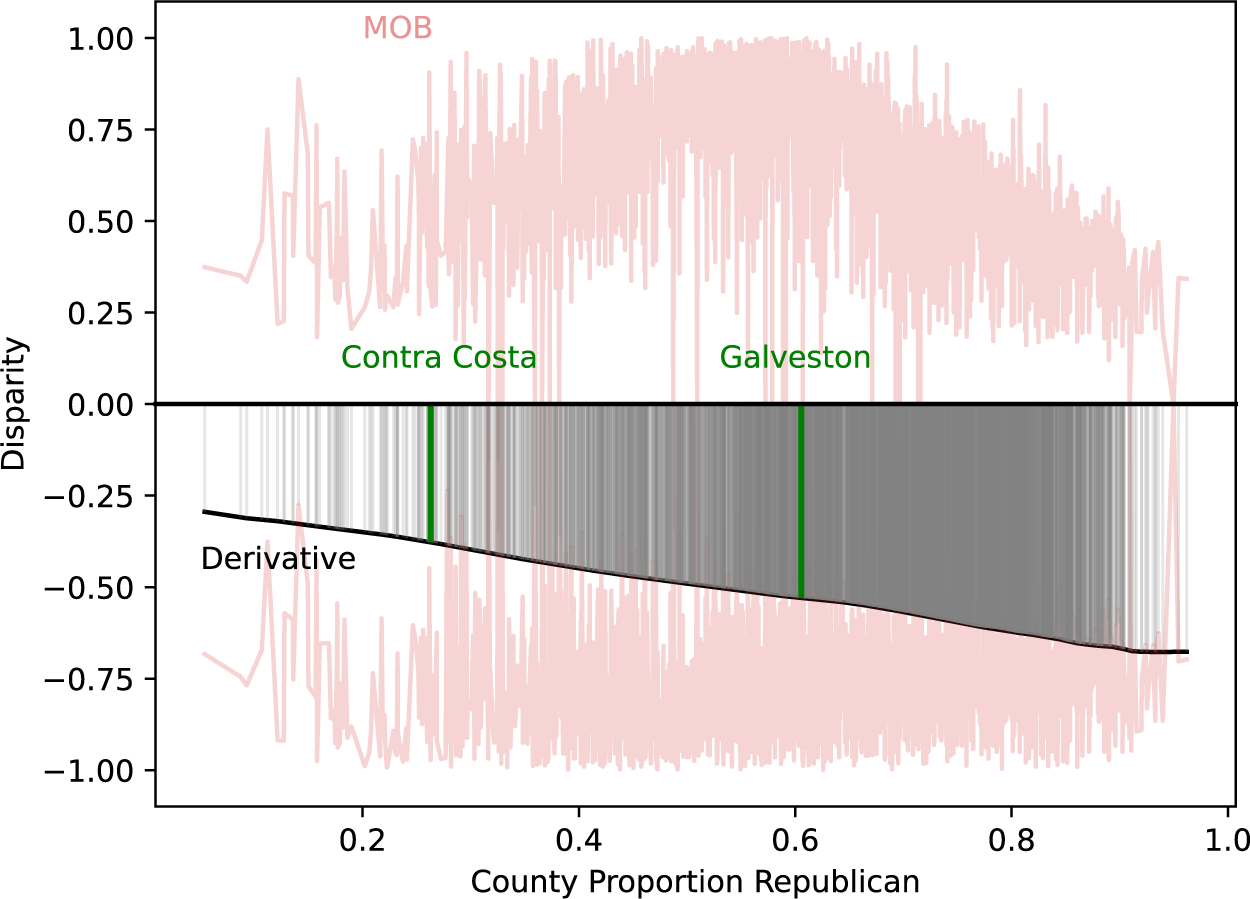
Finally, monotone EI may also be used to more precisely bound county-specific vaccine disparities. For purposes of this exercise, we assume that contextual reinforcement holds locally for each county: that is, $\delta _{B,n} \cdot \delta _{W,n}\geq 0$ for all n. To calculate the implied bounds from Proposition 9, we estimate $\mu '(X_n)$ using population-weighted local linear approximation (Figure S3 in the Supplementary Material). For Contra Costa County, which leans left-of-center politically, we estimate that the vaccination rate for Republican voters is between 0.50 and 0.77 and that the vaccination rate for Democratic voters is between 0.77 and 0.87. For Galveston County, which leans right-of-center politically, the respective bounds for Republicans and Democrats are from 0.36 to 0.57 and from 0.57 to 0.89. Each of these intervals is substantially narrower than the corresponding interval derived from the MOB (see Figure 4).

Figure 4

County-specific bounds.

Note: This figure shows the method of bounds for the partisan vaccination gap for each county (red). The county-level bounds, based on the assumptions in Proposition 9, are shown in gray, and the estimated derivative of the conditional expectation function of the vaccination rate by county partisan makeup is shown in black. The implied bounds for Contra Costa County, California, and Galveston County, Texas, are highlighted in green.

Figure 4. Long description

The x-axis is labeled County Proportion Republican, ranging from 0 to 1. The y-axis is labeled Disparity, ranging from -1 to 1. Two dense, jagged, connected red series labeled MOB form bands corresponding to the method of bounds for the partisan vaccination gap across counties and span roughly from -1 to 1. Vertical gray bars represent county-level bounds based on Proposition 9 assumptions, with a solid black line indicating the estimated derivative of the conditional expectation function of vaccination rate by county partisan makeup. Two vertical green lines highlight the positions of Contra Costa County, California (left, near 0.3), and Galveston County, Texas (right, near 0.6). The word Derivative appears in bold black text in the lower left. The overall trend in the derivative is a gradual decrease from left to right and is always negative, indicating a negative relationship between Republican proportion and vaccination rate disparity.