


1. Introduction
The knowledge of today's glacier ice thickness and parameters governing ice flow is crucial to initialize prognostic glacier or ice-sheet models (e.g. Perego and others, Reference Perego, Price and Stadler2014; Mosbeux and others, Reference Mosbeux, Gillet-Chaulet and Gagliardini2016; Goelzer and others, Reference Goelzer2018), which can predict their future evolution under climate change, and the resulting consequences, e.g. in terms of sea-level rise (Marzeion and others, Reference Marzeion2020; Edwards and others, Reference Edwards2021). Reconstructing the ice thickness of a glacier (or equivalently the bedrock elevation) is an active research topic in glaciology that involves direct measurement techniques – typically ground penetrating radar (Rutishauser and others, Reference Rutishauser, Maurer and Bauder2016) – and a large diversity of methods (see Farinotti and others, Reference Farinotti2017, for an overview) to produce estimates where no direct data are available. These methods usually rely on observable data such as surface ice topography, surface mass balance, surface ice flow speeds, ice thickness change or a combination of these.
The majority of the existing methods rely on the inversion of mass conservation and/or on the inversion of approximations of the conservation of momentum associated with Glen's flow law (Glen, Reference Glen1953). The two approaches are intrinsically very different as they take different input data (namely, mass balance and ice thickness change versus surface ice speeds) and involve two different types of equations. Advantageously, the conservation of momentum equation is time independent unlike mass conservation, avoiding dealing with climate variability when using the second approach. Choosing the first and/or the second is generally a matter of data availability.
In the first approach, a classical method (e.g. Farinotti and others, Reference Farinotti, Huss, Bauder, Funk and Truffer2009; Morlighem and others, Reference Morlighem2011; Fürst and others, Reference Fürst2018; Maussion and others, Reference Maussion2019) is used to reconstruct ice fluxes from the estimated mass balance/ice surface changes by integrating the divergence of the flux and deducing the ice thickness from the shallow ice approximation (SIA). A key advantage of this approach is that mass balance (unlike ice flow) can be estimated by modeling without any prior knowledge of the sought ice thickness, and this can be generalized at a global scale (Farinotti and others, Reference Farinotti2019). However, this approach suffers from uncertainties in the ice-flux reconstruction and shortcomings in the SIA. Indeed, the SIA neglects essential components of the stress in the case of mountain glaciers, which feature significant basal motion and/or steep bedrock even if the aspect ratio of the ice geometry is small (Le Meur and others, Reference Le Meur, Gagliardini, Zwinger and Ruokolainen2004).
In the second approach, there exist various inversions of the ice flow mechanics at different complexity levels including the SIA (e.g. Gantayat and others, Reference Gantayat, Kulkarni and Srinivasan2014; Michel-Griessera and others, Reference Michel-Griesser, Picasso, Farinotti, Funk and Blatter2014), the shallow shelf approximation (Goldberg and Heimbach, Reference Goldberg and Heimbach2013), or three-dimensional high-order models like Blatter or Stokes (Perego and others, Reference Perego, Price and Stadler2014). The inversion of non-SIA models is traditionally performed using an adjoint-based gradient method to iteratively calculate basal conditions that minimize the misfit with observations (Kirner, Reference Kirner2007). While these methods proved to be efficient in retrieving optimal basal friction conditions alone (e.g. Gagliardini and others, Reference Gagliardini2013; Morlighem and others, Reference Morlighem, Seroussi, Larour and Rignot2013; Mosbeux and others, Reference Mosbeux, Gillet-Chaulet and Gagliardini2016), the simultaneous optimization of ice thickness and sliding parametrization is rather rare (Goldberg and Heimbach, Reference Goldberg and Heimbach2013; Perego and others, Reference Perego, Price and Stadler2014). The latter work also includes a misfit of the flux divergence to account for mass conservation, which ensures an equilibrium between ice dynamics and mass balance, and limits nonphysical effects at the initialization of the transient model (referred to as ‘shock’ in the following discussion). However, adjoint methods present several difficulties: (1) the derivation of the adjoint problem is cumbersome, (2) purely deterministic gradient methods are prone to be locked into a local minimum affecting the robustness of the method to find the global minimum, and (3) the method is usually computationally expensive since it requires running the forward model many times until convergence is reached. To address the first issue, automatic differentiation has been successfully applied for parameter and state estimation in a time-dependent marine ice-sheet model (Goldberg and Heimbach, Reference Goldberg and Heimbach2013).
When available, surface ice-flow speed is a key measurement that is required when solving an inverse problem for ice thickness or/and basal conditions. Indeed, the dynamics of ice solely depend on the glacier geometry, basal conditions and internal viscosity at a given time, and has negligible dependence on time in the case of temperate glacier ice. Therefore, knowing the surface topography and velocities in three dimensions at a given time is theoretically sufficient to determine the ice thickness by inverting an ice flow model for the given ice flow parameters and under regularity assumptions. Furthermore, there is an inherent benefit in using glacier flow compared to surface ice fluxes as forcing data for the inversion because internal glacier fluxes are more stable than surface ice fluxes, which fluctuate with climate variability. Until recently, the observed surface ice flow field was sparsely available, explaining why these key data have been rarely exploited to date. However, recent advances in remote sensing techniques to capture horizontal glacial flow promise increasing observation coverage (e.g. Scambos and others, Reference Scambos, Fahnestock, Moon, Gardner and Klinger2016; Friedl and others, Reference Friedl, Seehaus and Braun2021; Millan and others, Reference Millan, Mouginot, Rabatel and Morlighem2022), opening new perspectives for ice thickness inference globally.
The complexity and computational costs of inversion methods for high-order ice flow models (Blatter or Stokes) as well as the lack of observed velocity data hinder their generalization at a large scale and the possibility to optimize several variables simultaneously. In this paper, we take advantage of a new global dataset for surface ice flow speeds (Millan and others, Reference Millan, Mouginot, Rabatel and Morlighem2022), and present a new method to simultaneously seek ice thickness and basal conditions of valley glaciers by inverting an emulated Stokes ice flow model in form of the convolutional neural network (CNN) proposed by Jouvet and others (Reference Jouvet2021). Doing so with a CNN emulator instead of a traditional Stokes model has two major advantages (i) automatic differentiation techniques avoid the manual derivation of an adjoint problem and (ii) once trained, CNNs are computationally inexpensive, especially with graphics processing unit (GPU) considerably speeding-up their evaluation. We test our method on ten of the largest glaciers in Switzerland, for which all necessary forcing and validation data are available.
Like in many other disciplines, machine learning has attracted a lot of interest in glaciology in the last few years for diverse applications such as the modeling of surface mass balance (Bolibar and others, Reference Bolibar, Rabatel, Gouttevin, Zekollari and Galiez2022) or the analysis of remote-sensing glacier-related products (Mohajerani and others, Reference Mohajerani, Wood, Velicogna and Rignot2019). The use of artificial neural networks (ANNs) for estimating basal conditions – and the bedrock location in particular – is not new (Clarke and others, Reference Clarke, Berthier, Schoof and Jarosch2009). Recently, Leong and Horgan (Reference Leong and Horgan2020) used a generative model based on a neural network to downscale existing reconstructed basal topography of Antarctica in high-resolution. Haq and others (Reference Haq, Azam and Vincent2021) used an ANN trained from a digital elevation model and glacier extent data to estimate the ice thickness of individual glaciers. A few studies have worked at including ice flow physics in data-driven neural networks to infer the bedrock topography (Monnier and Zhu, Reference Monnier and Zhu2021) or slippery information (Riel and others, Reference Riel, Minchew and Bischoff2021). Lastly, Brinkerhoff and others (Reference Brinkerhoff, Aschwanden and Fahnestock2021) used a neural network to emulate an expensive coupled ice flow/subglacial hydrology model, and infer the optimal parameters that best reproduce the observed surface velocities using a Bayesian approach.
In the following, we first describe our data assimilation method including the data generation with a Stokes model, the training and inversion of the resulting ice flow emulator. Then, we present ice thickness reconstructions for an ensemble of ten glaciers with different variants of the optimization method, and assess their performance. Lastly, we discuss our results and the potential of the method for global glacier modeling.
2. Methods
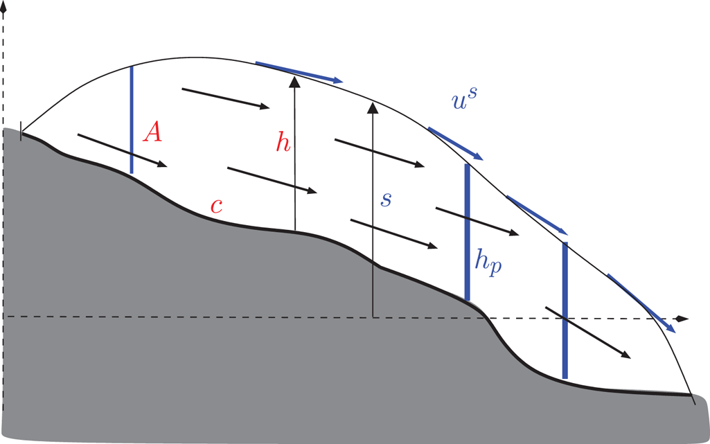
Here we denote b(x, y), h(x, y, t) and s(x, y, t) = b(x, y) + h(x, y, t) the bedrock elevation, ice thickness and ice surface elevation, respectively. We call $\bar {\bf u} = ( \bar {u},\; \, \bar {v})$ and us = (u s, v s) the vertically-averaged and surface horizontal ice velocity fields (Fig. 1). We assume the horizontally modeled domain to be a rectangle, which is subdivided by a regular 2D grid with uniform spacing in x and y – the variable h, s, b, $\bar {u}$
 , $\bar {v}$
 , u s, v s being defined at the center of each cell.
Cross-section of a glacier with annotations. The data assimilation consists of finding ice thickness distribution h and ice flow parametrization (c, A) (red) variables, which optimize the match with observational (blue) variables such as surface elevation, surface velocity (materialized by arrows) or measured ice thickness profiles.
In the following, we first review the Stokes instructor model, how it is used to generate data, and how the data are used to train the ice flow emulator. As this workflow was already described (Jouvet and others, Reference Jouvet2021), we refer to this paper for details and only provide a short description in the following section. Then, we describe our method to invert the ice flow emulator, which is the key contribution of this paper.
2.1. Stokes instructor model
To train our deep learning-based ice flow emulator, we carry out an ensemble of simulations to generate a large dataset of glacier dynamical states using a time-evolution glacier model based on Stokes equations (Jouvet and others, Reference Jouvet, Picasso, Rappaz and Blatter2008). The ice deformation is modeled by coupling the momentum conservation equation to Glen's flow law (Glen, Reference Glen1953):

where D is the strain rate tensor, τ is the deviatoric stress tensor, A is the so-called rate factor (a parameter that controls the ice viscosity), and n = 3 is Glen's exponent. On the other hand, basal sliding is modeled with a nonlinear sliding law – known as Weertman's law (Weertman, Reference Weertman1957):

where u b is the norm of the basal velocity, τ b is the basal shear stress, and c is a constant sliding coefficient.
While the Stokes equations are solved by finite elements, the glacier surface evolution is obtained by solving a transport equation for the volume of fluid, which proved to be a robust method to model the time evolution of complex glacier shapes (Jouvet and others, Reference Jouvet, Picasso, Rappaz and Blatter2008). Here, we used a simple mass-balance model, which is a linear function of the elevation with accumulation and ablation vertical gradients of 0.005 and 0.009 a−1, respectively, and maximum accumulation rates of 2 m a−1. The advance and retreat of the glacier is forced by the equilibrium line altitude (ELA).
The Stokes model has two critical parameters that control the ice flow; the sliding coefficient c and the rate factor A in Glen's law, which is a function of the ice temperature. The simultaneous inference of A and c from the observed surface velocity leads to nonunique solutions (both shearing or sliding dominant flows producing similar surface speeds) in the absence of additional discriminating data. Therefore an additional constraint on the relationship between A and c must be imposed on the problem in order to find a unique solution.
In this paper, we formulate this assumption from the following statement: basal motion is unlikely (respectively likely) to append when the ice is cold (respectively temperate) at bed. This translates into the assumption that either c = 0 km MPa−3 a−1 and A < 78 MPa−3 a−1 for cold ice, or c > 0 for A = 78 MPa−3 a−1, for temperate ice, which is the typical value at pressure-melting point (Cuffey and Paterson, Reference Cuffey and Paterson2010). Under this assumption, we can reduce the two parameters A and c to a single one

where λ = 1 km−1 is set arbitrarily (which is not a problem since $\tilde {A}$ is tuned to data), and therefore force the optimization problem to be well-posed. The new parameter $\tilde {A}$
 should be understood as a generic control on the ice flow strength; raising this parameter permits one to describe regimes from non-sliding and low shearing cold ice (low A, c = 0) to fast and sliding dominant temperate ice (A = 78 MPa−3 a−1, and high c), with $\tilde {A} = 78$
 MPa−3 a−1 representing a mid-way value corresponding to non-sliding and shearing temperate ice (A = 78 MPa−3 a−1, c = 0 km MPa−3 a−1), as represented in Figure 2. While $\tilde {A}$
 is defined by (3), (A, c) can be inferred from $\tilde {A}$
 :
:

While constant values for A and c (and then for $\tilde {A}$ ) are taken for training, we allow $\tilde {A}$
 to vary spatially (i.e. $\tilde {A} = \tilde {A}( x,\; \, y)$
 ) for the inversion later on to permit a local control of the ice flow strength. However, it must be stressed that $\tilde {A}$
 does not depend on z (i.e. it represents the depth-average value). The counterpart of this assumption is that the dynamics of an ice layer, which shows a cold surface and temperate base (Greve and Blatter, Reference Greve and Blatter2009), is approximated with an intermediate control value $\tilde {A}$
 , which averages low A (due to cold ice) and c > 0 (due to basal sliding). Note that the inversion method presented in this paper is not conditioned to this assumption, and that other constraints on the pair (A,c) can be enforced.
In this paper, the ice flow strength is controlled by a single parameter $\tilde {A} = A + \lambda c$ , where A is the rate factor in Glen's flow law that controls the ice shearing from cold-ice case (low A) to temperate ice case (A = 78 MPa−3 a−1), c is a sliding coefficient that controls the strength of basal motion from no sliding (c = 0) to high sliding (high c) and λ = 1 km−1 is a given parameter.

2.2. Data generation
Equipped with the Stokes instructor model, the goal is now to construct diverse dynamical states to obtain a heterogeneous dataset that describes large/narrow, thin/thick, flat/steep, long/small glaciers that can be met in future modeling. For that purpose, we have taken existing valleys from the European Alps and New Zealand, that are today ice-free but were likely covered by ice during the last glaciation, and prescribed mass-balance conditions to build glaciers there. In more detail, we have picked ten diverse valleys with drainage basins ranging from 80 to 700 km2, which have proved to produce an heterogeneous dataset (Jouvet and others, Reference Jouvet2021). For each one, we built a 100 m resolution two-dimensional structured mesh and projected it in three dimensions onto the digital elevation model (DEM) from the NASA Shuttle Radar Topographic Mission (SRTM, http://srtm.csi.cgiar.org/). A three-dimensional mesh was then vertically extruded with 10 m thick layers. All simulations were initialized with ice-free conditions, and the model was run forward-in-time for 100 years using a low ELA to allow glaciers to grow and advance. After 100 years, the glacier has spread over most of the drainage basin. Then, the ELA was raised for the next 100 years to let the glacier retreat. Runs were carried out with varying parameters (A, c) (or $\tilde {A}$ ):
):

or

to describe a large range of ice flow from slow shearing to rapid sliding (Fig. 2). Note that A =11, 30, 54, 78 MPa−3 a−1 corresponds to the rate factor for ice at − 10, − 5, − 2 and 0°C, respectively (Cuffey and Paterson, Reference Cuffey and Paterson2010).
2.3. Ice flow emulator
Following Jouvet and others (Reference Jouvet2021), our ice flow emulator predicts vertically average and surface horizontal velocity from ice thickness, surface slope and ice flow strength parameter $\tilde {A}$ :
:

where input and output are two-dimensional fields, which are defined over the discretized computational domain (or subparts) of size N X × N Y. The above emulator is the one introduced by Jouvet and others (Reference Jouvet2021) but augmented with the surface velocity in the output variable set as necessary to define a misfit with observations.
We approximate ${\cal F}$ by means of an ANN, which maps input to output variables using a sequence of network layers connected by trainable linear and non-linear operations with weights, which are adjusted (or trained) to a dataset. Here we use a CNN (Long and others, Reference Long, Shelhamer and Darrell2015), which is a special type of ANN that additionally includes local convolution operations to extract translation-invariant features as trainable objects and then learn spatially-variable relationships from given fields of data (LeCun and others, Reference LeCun, Bengio and Hinton2015). CNNs are therefore suitable to learn from a high-order ice flow model, that determines the velocity solution from topographical variables and their spatial variations.
Here, we used the network architecture from Jouvet and others (Reference Jouvet2021), which was found to be optimal in terms of model fidelity to number of parameters. At training, we minimize the sole L 1 loss function using a stochastic gradient method – the Adam optimizer (Kingma and Ba, Reference Kingma and Ba2014) – with a learning rate of 0.0001, a batch size of 64 and 200 epochs (or iterations) to reach convergence. As a result, the CNN is several orders of magnitude cheaper to evaluate than the original Stokes problem, with fidelity levels above 90% provided the solution is in the ‘hull'of the training dataset. In other words, one has to make sure that the glacier to be modeled has some close analogs in terms of size, thickness, slope and speed in the pool of training glaciers. Here our emulator is suitable for mountain glaciers thinner than 800 m, but not for thicker ice caps or ice sheets.
In contrast, fast flowing ice with a larger spatial dependence as found in tidewater glaciers and ice shelves (not considered here) might be better learned with more elaborated multiscale architectures such as the U-Net one (Ronneberger and others, Reference Ronneberger, Fischer and Brox2015). The latter has not been selected here as it did not show any superiority over CNNs for local mountain glacier-like flow. The Python code for training CNN and U-Net is publicly available at https://github.com/jouvetg/dle, and can be used to manufacture specific ice flow emulators from modeled data.
2.4. Inversion algorithm
In this section, we present the optimization method to simultaneously seek optimal input fields h, $\tilde {A}$ and s of the ice flow emulator (Eqn (4)) that fit the best given observations including: (i) observed ice surface velocities ${\bf u}^{{\rm obs}}_s = ( u_s^{{\rm obs}},\; \, v_s^{{\rm obs}})$
 , (ii) ice thickness profiles $\{ h_p^{{\rm obs}},\; \, p \in [ 0,\; \, \ldots ,\; \, P] \}$
 at given locations (each h p is defined along a given measured profile $\{ ( x^p_i,\; \, y^p_i) ,\; \, i = 1,\; \, \ldots ,\; \, M_p \}$
 ) (iii) top ice surface s obs, and (iv) an ice-free mask ${\cal M}^{\rm ice}\hbox{-}{\rm free}$
 , and/or (iv) observed flux divergence d obs obtained from surface mass balance and ice thickness change. Our choice to include the top ice surface field s as an optimization variable allows accounting for possible observation errors of s obs or time shift between data (e.g. ${\bf u}^{{\rm obs}}_s$
 and s obs may refer to slightly different years).
Here, we closely follow Perego and others (Reference Perego, Price and Stadler2014) by setting up a cost function ${\cal J}$ , which represents the difference between modeled and observed variables. The key difference with Perego and others (Reference Perego, Price and Stadler2014) is that the modeled velocity field is the output of a trained ANN instead of the direct solution of a physical ice flow model. As the problem is usually not well-posed (several combinations of ice thickness and ice flow parameters yield the same surface velocities), we additionally impose smoothness constraints to h and $\tilde {A}$
 by using regularization terms. The least square optimization problem consists of finding spatially varying fields h, $\tilde {A}$
 and s that minimize the cost function

where

is the misfit between modeled and observed surface ice velocities (${\cal F}$ is the output of (4)),

is the misfit between modeled and observed ice thickness profiles,

is the misfit between the modeled and observed top ice surface,

is a misfit term between the flux divergence $\nabla \cdot ( h {\bar {\bf u}})$ and its polynomial regression d poly with respect to the ice surface elevation s(x, y) to enforce smoothness with linear dependence to s,

is a regularization term to enforce anisotropic smoothness and convexity of h (see next paragraph),

is a regularization term to enforce smooth $\tilde {A}$ , and
, and

is a penalty term to enforce nonnegative ice thickness. Here $\tilde {{\bf u}}_s^{{\rm obs}}$ in Eqn (10) is the observed surface velocity field ${\bf u}_s^{{\rm obs}}$
 after applying a Gaussian smoothing (σ = 3) and normalizing, and $( \tilde {{\bf u}}_s^{{\rm obs}}) ^{\perp }$
 is its orthogonal field. Lastly, we denote σ u, σ h, σ d, σ s as the user-defined confidence levels (possibly spatially varying) errors of observations for ${\bf u}_s^{{\rm obs}}$
 , $h_p^{{\rm obs}}$
 , d obs and s obs, respectively, and $\alpha _h,\; \, \gamma ,\; \, \alpha _{\tilde {A}}> 0$
 , 0 < β < 1 are fixed parameters.
In the above definition of ${\cal J}$ , the choice of the regularization term ${\cal R}^h$
 of the ice thickness h defined by (10) is motivated by the following statements:
(i) Glacier beds (or equivalently ice thicknesses) are in general smoother along the ice flow direction than in the across direction due to glacial erosion.
(ii) In the absence of data for ice thickness, the convexity of ${\cal J}$
 can be artificially enforced in the early stages of the iterative optimization scheme to facilitate convergence.

To account for (i), we have projected the gradient of the ice thickness along flow direction and the orthogonal to obtain directional derivatives and enforce smoothing of h in an anisotropic way, i.e. we impose further smoothness along the ice flow direction – the anisotropy being controlled by user-defined parameter 0 < β < 1. To account for (ii), ${\cal R}^h$ includes the term $-\int _{\Omega } \gamma h$
 that aims at enforcing a slight convexity (controlled by parameter γ) of the ice thickness when no observational data are available to aid convergence without impacting the optimal solution. Heuristically, β = 1 minimizing ${\cal R}^h$
 (i.e. $\int \vert \nabla h \vert ^2 - \gamma h$
 ) is equivalent to solving the Euler–Lagrange equation − Δh = γ, which is the well-known Poisson problem with loading γ.
Lastly, we have imposed a smooth flux divergence through the regularization term ${\cal C}^{d}_{{\rm poly}}$ defined by (9) in ${\cal J}$
 to counter non-physical oscillations (Fig. 8). On the other hand, the linear dependence in z we imposed is a common feature of mass balance and elevation change of mountain glaciers. However, when observation of the divergence flux is available d obs, we may replace ${\cal C}^{d}_{{\rm poly}}$
 by:
by:

Note that the flux divergence $\nabla \cdot ( h {\bar {\bf u}})$ is approximated by finite-difference using an upwind first-order scheme similar to the solving of the mass conservation equation in the glacier evolution model (Appendix A, Jouvet and others, Reference Jouvet2021).
We have written the above optimization problem in the most general case for convenience, however, it is straightforward to optimize only for h or $\tilde {A}$ if information on one of the variables is already known, or in case the system is under-constrained by lack of data to define the cost function. Indeed, while ice surface velocity data ${\bf u}^{{\rm obs}}_s$
 are now available globally (Millan and others, Reference Millan, Mouginot, Rabatel and Morlighem2022), measured ice thickness profile data are only available for sparse sites. In case these data are not available, we would fix $\tilde {A}$
 and optimize for the ice thickness h only as it is a stronger control.
The above-mentioned optimization problem is solved using a stochastic gradient descent method with adaptive learning rate, namely, the Adam optimizer (Kingma and Ba, Reference Kingma and Ba2014). For that purpose, gradients of ${\cal J}$ with respect to the input variables $h,\; \, \tilde {A},\; \, s$
 are obtained by automatic differentiation. The optimization scheme is stopped when the cost function no longer decreases. The Adam scheme is initialized with zero ice thickness h = 0 and constant $\tilde {A} = 78$
 MPa−3 a−1, which corresponds to the neutral non-sliding temperate ice shearing case (Fig. 2), and observed ice surface s = s obs.
2.5. Implementation
The optimization is implemented within the framework of the ‘Instructed Glacier Model’ (IGM, https://github.com/jouvetg/igm) (Jouvet and others, Reference Jouvet2021), which is a Python open-source code based on the Tensorflow library (https://www.tensorflow.org), and which can be used for prognostic glacier simulations based on the ice flow emulator (Eqn (4)). IGM runs both on central and graphics processing units (CPU and GPU). To automatically differentiate ${\cal J}$ with respect to the input variables $h,\; \, \tilde {A},\; \, s$
 , TensorFlow records all operations and the derivatives from inputs to the cost function ${\cal J}$
 . Then, during the backward pass, TensorFlow goes through this list of operations in reverse order to compute gradients with a chain rule of derivatives.
3. Results
We tested our method on ten of the largest Swiss glaciers, which feature an impressive number of available measurements: Grosser Aletsch, Unteraar, Rhone, Corbassière, Oberaletsch, Zmutt, Findelen, Trift, Otemma and Zinal Glaciers. It must be stressed that none of these glaciers were used for training the ice flow emulator, however, all of them are in the ‘hull’ of the training dataset (i.e. they have close analogs in the dataset). While the Grosser Aletsch Glacier spreads over ~ 80 km2 and has ~ 12 km3 of ice, the nine others are several times smaller: their areas range between 12 and 22 km2, and their estimated volumes range between 0.7 and 3 km3 (Grab and others, Reference Grab2021). For all these glaciers, the following measurements are available:
(i) observed surface ice velocities (${\bf u}_s^{{\rm obs}}$
) from Millan and others (Reference Millan, Mouginot, Rabatel and Morlighem2022), corresponding to the 2017–2018 time period, and with σ u = 5 m a−1 as confidence level,(ii) glacier surface DEMS (s obs) from swisALTI3D (www.swisstopo.admin.ch), corresponding to the 2016–2017 time period, and with σ s = 5 m as confidence level,
(iii) ice thickness profiles ($h_p^{{\rm obs}}$
) and their confidence errors σ h from ground-penetrating radar from Grab and others (Reference Grab2021) (these ice thickness profiles were homogenized by subtracting glacier bed elevation profiles data from the swisALTI3D DEM so that they all refer to 2016–2017),(iv) glacier outlines, and resulting mask ${\cal M}^{\rm ice\hyphen free}$
from the Swiss Glacier Inventory 2016 (Linsbauer and others, Reference Linsbauer2021) (this inventory may refer to the years preceding 2016, which is justifiable, as the given outlines serve to discriminate ice-free areas, and all considered glaciers have been shrinking in the past recent years).


For a single experiment on the Rhone and Grosser Aletsch Glaciers, we additionally use mass-balance data averaged between 2001 and 2016–2017 from GLAMOS (2020) as well as ice thickness change data based on DEM differentiation (2001 and 2016–2017 available from SwissTopo, www.swisstopo.admin.ch) to produce an observed flux divergence field d obs with σ d = 1 m a−1 as the confidence level.
We now report the results of seven different optimization schemes (defined in Table 1) including the most general form (hereafter denoted Optimization O or Opt. O) and six variants that exclude terms in the cost function and in the pool of optimization variables (i.e. controls) to assess the added value of each. For convenience, we named variants with the general form name O, but specified in the index the variable or constraint that was removed with an explicit minus symbol (e.g. O −d) whenever possible. With exception of the second scheme (Opt. $O^\ast$ ) that is applied only to the Rhone and Grosser Aletsch Glaciers, while all others are performed for all ten glaciers:
(i) Opt. O is the most general optimization scheme, which consists of seeking $( h,\; \, \tilde {A},\; \, s)$
that minimize the full cost function ${\cal J}$ defined by (5).(ii) Opt. $O^\ast$
replaces ${\cal C}^{d}_{{\rm poly}}$ defined by (9) in Opt. O by ${\cal C}^{d}_{{\rm obs}}$ defined by (13) to impose data fitting of the flux divergence instead of smoothness. Here, the motivation is to verify how much prior knowledge on the flux divergence permits preserving the equilibrium between ice dynamics and mass balance better than an assumption on its spatial regularity.(iii) Opt. O −d removes the flux divergence ${\cal C}^{d}_{{\rm poly}}$
in the cost function of O to quantify the resulting disequilibrium between ice dynamics and mass balance and conclude the added-value of ${\cal C}^{d}_{{\rm poly}}$.(iv) Opt. O −s is a variant of O, which removes the ice surface term ${\cal C}^s$
from the cost function and variable s from controls to assess the impact of ice surface adjustment.(v) Opt. $O_{-\tilde {A}}$
assumes $\tilde {A} = 78$ MPa−3 a−1 and removes $\tilde {A}$ from controls of O to assess the importance of optimizing along ice flow strength parametrization $\tilde {A}$.(vi) Opt. $O_{-\tilde {A}, \, h}$
is a variant of $O_{-\tilde {A}}$, which further removes ${\cal C}^h$ from the cost function, i.e. it does not use any measured ice thickness profiles, considering that such data only exist for a restricted number of glaciers.(vii) Opt. $\overline {O}$
takes the reconstructed ice thickness h from Grab and others (Reference Grab2021), and optimizes the variables $\tilde {A}$ and s to fit observed ice surface and velocities while ensuring smooth flux divergence. The goal here is to verify if adjusting $( \tilde {A},\; \, s)$ from previously optimized ice thickness distributions is sufficient to assimilate the data with the same quality level.


Unless specified differently, we use parameters α h = 10.0, β = 0.2, γ = 0.001 and $\alpha _{\tilde {A}} = 1.0$ , and lead a sensitivity analysis to measure the impact of each one.
Name, data used and definition (controls and cost function) of all optimization schemes carried out in this paper. The first line indicates the reference scheme (O) to which other schemes are compared to. When h (respectively $\tilde {A}$ ) is not part of the optimization, we use the ice thickness reconstruction from Grab and others (Reference Grab2021) (respectively we assume constant $\tilde {A} = 78$
 MPa−3 a−1).

To measure the mass balance–ice dynamics equilibrium, we run the forward time-evolution model after optimization using the observed mass balance for 5 years from the optimal initial conditions, and track the ice thickness changes similarly to Perego and others (Reference Perego, Price and Stadler2014).
Figure 4 shows the evolution of the ice flow strength parametrization $\tilde {A}$ , the ice thickness distribution h, as well as the resulting surface ice flow velocity field us through the iterations of the optimization scheme O for the Rhone and Grosser Aletsch Glaciers, while Figure 5 shows the evolution of the ice thickness profiles towards the targeted ones for the Rhone Glacier. Figure 6 shows the evolution of each component of the cost function through the iterations of the optimization.
Observed velocity fields from Millan and others (Reference Millan, Mouginot, Rabatel and Morlighem2022), locations of ice thickness profiles compiled by Grab and others (Reference Grab2021) and of the outlines from Linsbauer and others (Reference Linsbauer2021) for the Rhone and Grosser Aletsch Glaciers.

Evolution of the ice flow strength parametrization $\tilde {A}$ (unit: MPa−3 a−1), the ice thickness distribution h (unit: m), as well as resulting surface ice flow velocity field us (unit: m a−1) through the iterations of the optimization problem (Opt. O) for the Rhone (a) and Grosser Aletsch (b) Glaciers. The mean value of $\tilde {A}$
 , as well as the standard deviation (STD) between modeled and observed fields is reported at each step.

Evolution of the ice thickness profiles (depicted in Fig. 3) through the iterations of the optimization problem (Opt. O).

Evolution of each component of the cost function ${\cal J}$ (once normalized between 0 and 1) through the iterations of the optimization problem (Opt. O) for the Rhone Glacier.

Figure 7 shows the optimal ice flow strength parametrization $\tilde {A}$ , ice thickness distribution h, as well as resulting surface ice flow velocity field us for the Rhone and Grosser Aletsch Glaciers, and for four optimization schemes (O, $O_{-\tilde {A}}$
 , $O_{-\tilde {A}, \, h}$
 and $\overline {O}$
 ). Figure 8 additionally shows the results of Opt. O, $O^\ast$
 , O −d, O −s for the Rhone Glacier, including further information in terms of flux divergence, ice top surface and equilibrium ice dynamics/mass balance. Figure 9 displays the ice thickness distribution of the eight other glaciers after optimization.
Optimal ice flow strength $\tilde {A}$ (unit: MPa−3 a−1), ice thickness h (unit: m), resulting surface velocity field us (unit: m a−1), and velocity difference based on Opt. O, $O_{-\tilde {A}}$
 , $O_{-\tilde {A}, \, h}$
 , and $\overline {O}$
 for the Rhone and Grosser Aletsch Glaciers.

Optimal ice flow strength $\tilde {A}$ (unit: MPa−3 a−1), ice thickness h (unit: m), ice velocity misfit (unit: m a−1), flux divergence misfit (unit: m a−1), ice surface misfit (unit: m), and ice thickness change over 5 years (unit: m) of forward model time integration based on Opt. O, $O^\ast$
 , O −d, O −s.

Ice thickness distribution of the eight remaining glaciers after optimization (Opt. O).

Lastly, Table 2 summarizes the results of optimizations O, $O_{-\tilde {A}}$ , $O_{-\tilde {A}, \, h}$
 and $\overline {O}$
 for all ten glaciers, i.e. it gives the standard deviation (STD) for ice thickness and ice velocity obtained at the end of the optimization procedure, as well as the ice volumes. Table 3 provides the same results for Opt. O, O −d, O −s with additional STDs for flux divergence and ice surface.
Results of optimizations O, $O_{-\tilde {A}}$ , $O_{-\tilde {A}, \, h}$
 and $\overline {O}$
 for all ten glaciers: Σh is the standard deviation (STD) between modeled and measured ice thickness profiles, $\Sigma _{u^s}$
 is the STD between modeled and measured ice surface velocities, ${{\cal V}}$
 is the total ice volume, $\bar {{\cal V}}^G$
 is the ice volume found by Grab and others (Reference Grab2021) relative to ${{\cal V}}$
 , $\Sigma _{h}^{G}$
 is the standard deviation between optimized thicknesses and the ones found by Grab and others (Reference Grab2021), $\bar {{\cal V}}$
 is the ice volume relative to ${{\cal V}}$
 . For Opt. $\overline {O}$
 we provide $\Sigma _{u^s}$
 without optimization ($\tilde {A} = 78$
 ) and after optimizing $\tilde {A}$
 .
.

Results of optimizations O, O −d, O −s for all ten glaciers. The meaning of each column is described in the caption of Table 2. In addition, $\oint \tilde {A}$ denotes the average of $\tilde {A}$
 over the glaciated area, Σd denotes the flux divergence STD and $\Sigma _{u^s}$
 denotes ice surface STD.

3.1. Reference optimization scheme O
For all glaciers, we found that the optimization scheme O converges efficiently (see examples in Figs 4 and 6) within a few hundred iterations with a smooth decrease and stabilization of cost components (the surface misfit and the regularization of $\tilde {A}$ take the longest to stabilize, Fig. 6). We additionally found that the descent scheme is robust with respect to initial states (not shown), i.e. taking different ice thicknesses h and ice flow strength $\tilde {A}$
 as the initial iterate leads to very similar final solutions. This shows that the regularization terms ensure the optimization problem to be well-posed and the algorithm to converge to a unique solution.
Inherent to the glacier size, STD between observations and optimized corresponding fields (called Σh, $\Sigma _{u^s}$ , Σd and Σs in Tables 2 and 3) demonstrate efficient data assimilation:
(i) The ice thickness STD Σh measuring the misfit in ice thickness varies between 4 and 11 m (Table 2). In the case of the Rhone Glacier, Figure 5 shows that the convergence of the ice thickness toward the targeted profiles is efficient except for the two last profiles, which show high variations and are underfitted – a situation that could be recovered by relaxing the regularity parameters α h and β.
(ii) The surface ice velocity STDs $\Sigma _{u^s}$
vary between 5 and 11 m a−1 (Table 2 and Fig. 7 for the Rhone and Grosser Aletsch Glaciers).(iii) Optimal solutions for the Rhone and Grosser Aletsch Glaciers show a fair match with the observed flux divergences (STDs are under 1 and 2 m a−1, respectively, Table 3), which implies the mass balance and the ice dynamics to be well balanced as witnessed by relatively small changes in the ice thickness after 5 years of integration of the forward model (Fig. 8).
(iv) The relaxation of the top ice surface (measured by the ice surface STD) always leads to relatively small adjustments within the uncertainty range σ s under 5 m, with two exceptions for Grosser Aletsch Glacier (9 m) and Unteraar (6 m).

Note that the higher misfit score of the Grosser Aletsch Glacier is simply the result of greater dimensions – both in terms of ice thickness and ice flow strength – as the scores are given in an absolute manner.
3.2. Ice flow strength parametrization
For all glaciers, the optimal ice flow strength parametrization field $\tilde {A}$ was found relatively close to the neutral value 78 MPa−3 a−1 on average (Table 3 and Fig. 4). Only the Grosser Aletsch Glacier shows a mean value higher than 78 ($\tilde {A}$
 =82), which is the consequence of high values over the tongue (Fig. 4) in the case of the Rhone Glacier. When fixing $\tilde {A} = 78$
 MPa−3 a−1, optimizing for the ice thickness and surface ice (h, s) only (Opt. $O_{-\tilde {A}}$
 ) does not significantly change the modeled ice thickness nor the ice flow field (Fig. 7) compared to Opt. O. Table 2 confirms the modest added-value of optimizing $\tilde {A}$
 in terms of STD reductions for the ice thickness of the ice velocity between Opts. O and $O_{-\tilde {A}}$
 (compare Σh and $\Sigma _{u^s}$
 in Table 2), and for all glaciers except Grosser Aletsch. Our results therefore support the fact that A = 78 and c = 0 are in general appropriate values to describe the ice flow of glaciers of the Alps, however, a higher value of c is preferable for Grosser Aletsch.
3.3. Ignoring ice thickness profile data
When fixing $\tilde {A} = 78$ MPa−3 a−1, optimizing for (h, s) only without using any ice profiles data in the cost function (Opt. $O_{-\tilde {A}, \, h}$
 ), the ice thickness reconstruction changes to some extent (Fig. 7): the ice thickness STD increases by a factor ~ 3 − 7 while the ice surface velocity STD remains fairly small (compare Σh and $\Sigma _{u^s}$
 for Opt. $O_{-\tilde {A}}$
 and $O_{-\tilde {A}, \, h}$
 in Table 2). The total volume estimate differs by 6%, with a variability of 14 % (Table 2), indicating a moderate bias. This is an important result as ice thickness profiles are in general rarely available at a global scale. Here we found that while ice profiles can strongly improve the estimation of the ice thickness locally, their relevance to retrieve the global ice volume is less significant at a global scale. Note that the remaining bias is directly controlled by our hypothesis on the $\tilde {A}$
 value; for instance, the +13% bias in terms of ice volume of the Grosser Aletsch Glacier between Opt. O and $O_{-\tilde {A}, \, h}$
 would be reduced to − 2% using the mean value $\tilde {A} = 82$
 MPa−3 a−1 found in Opt. O instead of $\tilde {A} = 78$
 MPa−3 a−1. Indeed, raising $\tilde {A}$
 induces an increase of the ice flow speed, which must be compensated by a decrease of the ice thickness to maintain the ice flux.
3.4. Added value of flux divergence and top surface constraints
Our reference scheme O imposes smoothness on the flux divergence without using any observational flux divergence data. Here we assess the added value of using mass-balance data (Opt. $O^\ast$ ), as well as the importance of these two terms (Opt. O −d and O −s). Our findings are:
(i) Comparing Opt. O and Opt. $O^\ast$
results show that both the flux divergence misfit ${\cal C}^{d}_{obs}$ and a well-tuned regularization term ${\cal C}^{d}_{poly}$ lead to a similar fit in terms of flux divergence STD and equilibrium between ice dynamics and mass balance as witnessed by the ice thickness change after 5 years of forward model time integration (Fig. 8).(ii) Not accounting for the flux divergence in the cost function (Opt. O −d) leads to nonphysical, high-frequency variations of the optimal flux divergence (Fig. 8) with a strong misfit with observations (Σd in Table 3), and this results in a strong shock when integrating the model over 5 years (Fig. 8).
(iii) Including the ice surface elevation as an additional control (allowing small adjustments within the uncertainty range) gives more slack to the optimization system and permits a better match of all targeted quantities such as ice surface velocity, ice thickness, and flux divergence (Fig. 8). In particular, small adjustments of the top ice surface greatly help in absorbing and damping the original high-frequency variations of the flux divergence (Fig. 8).


3.5. Comparison with other ice thickness reconstructions
Table 2 provides the resulting total ice volumes of the ten reconstructed glaciers (Fig. 9) and compares them with the reference volumes found by Grab and others (Reference Grab2021). As a result, the reference optimization scheme O yields to ice thickness distributions and ice volumes that are in line with those found by Grab and others (Reference Grab2021): STDs for the ice thickness are between 8 and 16 m, while the total ice volume is 7% lower on average with an STD of 14 % (Table 2). This relatively good match was expected as our two reconstructions involve the same ice profile data.
Figure 10 compares the ice thickness distribution obtained with Opt. $O_{-\tilde {A}}$ to reconstructions from Millan and others (Reference Millan, Mouginot, Rabatel and Morlighem2022), Grab and others (Reference Grab2021) and Farinotti and others (Reference Farinotti2019) for the Rhone and Grosser Aletsch Glaciers. Note that Millan and others (Reference Millan, Mouginot, Rabatel and Morlighem2022) used the surface ice flow speed data of Opt. $O_{-\tilde {A}}$
 , Grab and others (Reference Grab2021) used the ice thickness profile data of Opt. $O_{-\tilde {A}}$
 , while Farinotti and others (Reference Farinotti2019) derived a composite solution of several reconstructions. Again the distributed ice thicknesses from Grab and others (Reference Grab2021) are fairly in line with our reconstruction, while those from Farinotti and others (Reference Farinotti2019) show more discrepancies (the ice thickness distribution is less heterogeneous) but without significant bias. In contrast, the reconstruction of Millan and others (Reference Millan, Mouginot, Rabatel and Morlighem2022) is notably thicker.
The ice thickness distribution from Millan and others (Reference Millan, Mouginot, Rabatel and Morlighem2022), Grab and others (Reference Grab2021), Farinotti and others (Reference Farinotti2019) and the one optimized in this study, the corresponding modeled ice flow field, and the difference between the two. For the first ice thickness reconstruction, the results are shown with two parameters: $\tilde {A} = 78$ and $\tilde {A} = 25$
 MPa−3 a−1.

Additionally, Figure 10 compares the ice flow fields modeled with the Stokes-emulated model resulting from all ice thickness solutions. The difficulty of this comparison resides in the choice of $\tilde {A}$ : since all methods have their own calibration, the same value of the ice flow strength control $\tilde {A}$
 (assumed to be spatially constant here) may not be optimal for all reconstructions. A preliminary analysis has shown that $\tilde {A} = 78$
 MPa−3 a−1 was found close to optimal (in terms of STD between observed and modeled surface ice velocities) for both Grab and others (Reference Grab2021) and Farinotti and others (Reference Farinotti2019), but $\tilde {A}$
 had to be reduced to $\tilde {A} = 25$
 for Millan and others (Reference Millan, Mouginot, Rabatel and Morlighem2022) to compensate the thicker ice, otherwise the ice flow velocities are clearly too high (Fig. 10). Once this leveling is done, we compare all resulting ice flow patterns. As a result, the ice flow field from Millan and others (Reference Millan, Mouginot, Rabatel and Morlighem2022) is closer (STD 20 m a−1) to the targeted observation than Grab and others (Reference Grab2021) (STD 36 m a−1) and Farinotti and others (Reference Farinotti2019) (STD 30 m a−1) solutions. This was expected as only Millan and others (Reference Millan, Mouginot, Rabatel and Morlighem2022) make use of these observation data. For comparison, the solution obtained with Opts. $O_{-\tilde {A}}$
 (assuming $\tilde {A} = 78$
 ) and O (further optimizing $\tilde {A}$
 spatially) reduces this misfit to 14 and 11 m a−1, respectively. Note that our first observations of the Rhone and Grosser Aletsch Glaciers generalize to the entire glacier pool: STDs in ice flow speeds are twice higher with the ice thicknesses from Grab and others (Reference Grab2021) compared to those obtained with the $O_{-\tilde {A}}$
 scheme (Table 2).
Using the ice thickness distribution reconstructed by Grab and others (Reference Grab2021), we found that optimizing for $( \tilde {A},\; \, s)$ alone (Opt. $\overline {O}$
 ) permits reducing the misfit in ice surface velocities (Table 2), but not entirely compared to other schemes involving the ice thickness (compare Opt. O and $O_{-\tilde {A}}$
 to Opt. $\overline {O}$
 in Table 2). Additionally, the optimal field $\tilde {A}$
 is unrealistically high in some areas (Fig. 7), which can hardly be interpreted as the values may correct for imperfection of the ice thickness distribution. This experiment emphasizes that the ice thickness field h is a stronger control on the ice velocity than $\tilde {A}$
 and highlights the necessity to include h as a control for data assimilation.
3.6. Regularization parameter sensitivity analysis
Figure 11 shows the impact of each individual parameter among α h, β, γ, $\alpha _{\tilde {A}}$ and α d for Opt. O on the Rhone Glacier. Each snapshot shows the optimization result with default parameters α h = 10, β = 0.2, γ = 0.001, $\alpha _{\tilde {A}} = 0.1$
 with exception of the one investigated. As a result, our findings are:
(i) Values of α h, which controls the smoothness of the ice thickness, close to ten yield the optimal STD reduction.
(ii) Values of β, which controls the smoothness degree along the flow direction, between 0.1 and 0.2, yield to the optimal STD reduction.
(iii) Values of γ, which enforces the convexity of the cost function, below 0.002 have nearly no impact on the solution. Furthermore, we found that the algorithm never moves out h = 0 (the initial state) when γ = 0 and when performing an optimization, which does not use any ice thickness profile data, presumably because the gradients of ${\cal J}$
are zeros at h = 0 in this case. In this case, a small (but non-zero) γ avoids this issue, and therefore augment the domain of convergence of the optimization scheme.(iv) Values of $\alpha _{\tilde {A}}$
, which controls the smoothness of $\tilde {A}$, have a very limited impact on the solution. We arbitrarily selected $\alpha _{\tilde {A}} = 0.1$ as default since it permits smooth variation over the ice domain.


Effect of parameters α h, β, γ on the optimized ice thickness (the three top panels) and parameter $\alpha _{\tilde {A}}$ on the optimized field of $\tilde {A}$
 (forth panel) for Opt. O of the Rhone Glacier.

3.7. Dealing with missing data
In the last experiment, we have applied Opt. $O_{-\tilde {A}, \, h}$ (i.e. using constant $\tilde {A} = 78$
 MPa−3 a−1, and not using any ice thickness profiles) to the Rhone Glacier, and using only a partial amount of the observed velocity field. In more details, we have disregarded 50, 80 and 90% of the available data in ${\cal C}^u$
 to mimic gaps in observations – the kept/rejected data being picked randomly (but uniformly). Additionally, we carried out the same experiment by disregarding a geometrical half part of the data (Fig. 12, top panel). The results of these experiments are depicted in Figure 12.
Restricted observed ice velocity, modeled ice thickness, ice velocity and the difference between the two (observed and modeled) ice velocities when removing observed ice velocity data from the constraints in the optimization problem for Opt. $O_{-\tilde {A}, \, h}$ (constant $\tilde {A} = 78$
 MPa−3 a−1, and without using any ice profiles).

As a result, we found that removing data homogeneously does not significantly affect the quality of the reconstructed ice thickness and ice flow up to the 80% removal level. In other words, the ice thickness STD remains nearly the same, while the ice velocity STD increases by only ~ 10% (Fig. 12). Only with 90% removal does the deterioration of the reconstruction quality becomes clearly noticeable. As expected, removing the data non-homogeneously leads to an uneven reconstruction quality. In contrast with the part with disregarded data, the remaining part is well reconstructed.
3.8. Computational performances
All optimizations were performed using a Python code based on the TensorFlow library embedded in the IGM. Computations were performed on the laptop-integrated NVIDIA Quadro P3200 GPU card (1792 1.3 GHz cores) and on a CPU (Intel(R) Core(TM) i7-8850H CPU with 6 2.6 GHz cores) for comparison purposes. Solving one inversion scheme Opt. O takes about 1 min per glacier on GPU, and roughly 2–5 times more on CPU according to the glacier size (the larger the domain, the more advantageous the GPU).
4. Discussion
Data assimilation is a key and challenging step to initialize prognostic glacier or ice-sheet evolution models (e.g. Goelzer and others, Reference Goelzer2018; Seddik and others, Reference Seddik2019). In general, data from the glacier surface (typically surface elevation and flow speed) are available by remote sensing, while information from the inside of the glacier is rarely available as it requires in situ measurements or from near-field remote sensing. The data assimilation step consists of seeking the interior conditions (typically the location of the bedrock and slipperiness information) that can best explain the surface data from physical modeling (Fig. 1), which relies on ice flow mechanics and mass conservation (MacAyeal, Reference MacAyeal1992).
In view of prognostic modeling, it is crucial to use the same physical model for data assimilation and direct ice flow modeling. Indeed, our results have shown that the ice thickness reconstructed with other embedded mechanics leads to Stokes-modeled ice velocity fields that are very different (Fig. 10). Initializing a prognostic ice flow model with these reconstructions would result in a shock with nonphysical transients effects. In turn, this would require performing an artificial relaxation to adjust the glacier surface to the modeled mechanics (e.g. Seddik and others, Reference Seddik, Greve, Zwinger, Gillet-Chaulet and Gagliardini2012) while the bedrock should be adjusted to the mechanics. While the local aspect of the SIA makes its inversion a relatively easy task, it is usually oversimplified for mountain glaciers characterized by significant basal motion and/or steep slopes as it neglects essential horizontal shear stresses. By contrast, high-order models account for these stresses, but their inversion is a complex and computationally expensive task (Perego and others, Reference Perego, Price and Stadler2014). The approach that we introduce in this paper precisely aims to considerably ease and speed up this task using CNN and automatic differentiation.
For that purpose, our strategy is to work with the trained CNN emulator introduced by Jouvet and others (Reference Jouvet2021) instead of the primary Stokes equations. Indeed, the gradient descent directions of the optimization problem are available by automatic differentiation (within the TensorFlow framework) and without having to derive manually and solve any adjoint problem. Using a stochastic gradient descent method together with an extra convexity term when no ice thickness profile is used in the cost function ensures efficient and robust convergence (Figs 4 and 6). Second, evaluating a neural network is several orders of magnitude cheaper than solving a Stokes problem, especially on GPU. Lastly, the loss in accuracy (10 %) of using an emulator instead of the Stokes equations is comparatively small (especially smaller than the uncertainty of the data to fit) should it be used within the ‘hull’ defined by the training dataset. The implementation of the optimization algorithm and its automatic differentiation tools is fairly simple thanks to the TensorFlow library with a speed-up of several order of magnitude compared to true Stokes-based inversion similar to the forward model (Jouvet and others, Reference Jouvet2021).
Besides its low cost, our method can easily handle multivariable optimization if there is enough data available to act as a constraint. Here we seek simultaneously for the optimum ice thickness, ice flow strength parameterization and ice top surface that allows a Stokes-emulated ice flow model to match a set of observations. As a result, the optimal solutions generally show very good data assimilation scores. For instance, in the case of the Rhone Glacier, we simultaneously match the ice thickness profiles, surface ice speed, top ice surface and flux divergence with STDs of 10 m, 9 m a−1, 4 m and 1 m a−1, respectively. Furthermore, all five regularization parameters tuned to the Rhone Glacier were found to be robust, e.g. they successfully applied to the nine other glaciers.
In all our experiments, ice thickness was always found to be a very strong control of the ice flow, so that the optimization scheme must perform fine adjustments to reach the optimal state. As an illustration of this, the ice thickness reconstructions – the ones from Grab and others (Reference Grab2021) and the ones optimized here – are both based on the same ice thickness profile data and are therefore rather close to each other (STD ~ 11 m, Table 2). However, the ice thickness distribution from Grab and others (Reference Grab2021) leads to a modeled ice flow field that is twice more distant to observations than the ice thickness optimized here (Fig. 10). By contrast, the ice flow strength parameterization $\tilde {A}$ as well as the ice surfaces were found to be second-order controls, and their tuning can reduce the misfit with observations, but only to a certain extent.
In theory, flux divergence observations (inferred from mass balance and ice thickness change) and surface ice flow speed observations would match if the model and observations were free of any errors. In practice, over-constraining the ice flow inversion by adding a constraint on the flux divergence (${\cal C}^{d}_{{\rm poly}}$ or ${\cal C}^{d}_{{\rm obs}}$
 ) allows a compromised solution to be found, which matches at best both types of observations (possibly contradictory) while being consistent with the mechanical model (Perego and others, Reference Perego, Price and Stadler2014). In our results, ignoring the flux divergence in the cost function always led to nonphysical high-frequency variations with a subsequent shock in the forward model. This undesired effect is the direct result of model and/or observation errors as explained above. However, we found that this artifact can be strongly damped by either constraining the flux divergence to fit the observations (${\cal C}^{d}_{{\rm obs}}$
 ), or by imposing it to be smooth (${\cal C}^{d}_{{\rm poly}}$
 , this second option is of special interest as it does not require any data) – both approaches lead to fairly similar results. Additionally, we found that adding any of these constraints affects the data assimilation quality but to a very limited degree. This demonstrates a general coherence of the optimized ice flow model with both types of observations (dynamics and flux divergence). As a corollary, it is not advisable to include the observed flux divergence data as an additional constraint in general if surface ice flow data are available. Indeed, flux divergence data observations are more prone to errors (as indirectly reconstructed) and more fluctuating in time than surface ice flow data inferred by remote sensing in a direct way. In fact, forcing smooth or observed flux divergence does not perform any data assimilation here, but instead permits us to deal with its deteriorated regularity, which is expected after applying the divergence operator.
Our method allows inference of the optimal spatially varying field $\tilde {A}$ , or equivalently the rate factor A and sliding coefficient c (even if they were spatially-constant at the training stage). Although both show some spatial variability, their average values remain close to A = 78 and c = 0 (Table 3), which is a commonly-used value for non-sliding temperate ice. Temperate ice is an expected feature for most of Alpine glaciers (Suter and others, Reference Suter, Laternser, Haeberli, Frauenfelder and Hoelzle2001). Only the Grosser Aletsch Glacier shows a mean value notably higher than 78 ($\tilde {A}$
 =82, or c=4). A closer look at the optimized field $\tilde {A}$
 (Fig. 4) reveals that the highest values of $\tilde {A}$
 (and then of c) are found over the glacier tongue – a feature that may be explained by the presence of subglacial melt water in the ablation area, with the result of promoting basal sliding. Further interpretation of the physical meaning of the optimal field A and c is tricky as some patterns (like the error pattern of the flux divergence) probably reflect shortcomings in our mechanical model.
Here we have applied our method to an ensemble of ten Swiss glaciers, for which a number of measured ice thickness profiles exist. While there exists now a global dataset of surface ice flow velocities (Millan and others, Reference Millan, Mouginot, Rabatel and Morlighem2022), ice thickness profile data are only available for a relatively small number of glaciers worldwide. Therefore, our most general optimization scheme O cannot be applied globally. When no ice thickness profile data are available, we proposed to remove field $\tilde {A}$ from controls (Opt. $O_{-\tilde {A}, \, h}$
 ) to preserve a balance between the number of controls and constraints. Here under the assumption of $\tilde {A} = 78$
 MPa−3 a−1 this alternative scheme leads to less accurate ice thickness reconstruction than expected, however, the error pattern on the ice volume suffers from fairly small biases (Table 2). In fact, the bias is directly controlled by the assumption made on $\tilde {A}$
 . We have demonstrated that our approach is robust enough to cover gaps in data up to 80–90% levels showing that it can be used as a physically based method to fill in missing data. In conclusion, our method has a great potential for deriving ice thickness fields of grounded glaciers at a global scale consistently with high-order ice flow mechanics.
There are a few challenges that must be addressed in view of generalizing the method at a global scale (i.e. without relying on ice thickness profile data), especially to take into account the diversity of glaciers. First, in absence of ice thickness data the key challenge is to tune $\tilde {A}$ , which is expected to vary in from site to site to account for the discrepancy in ice flow dynamics (e.g. due to subglacial hydrology or the presence of cold ice) and uncontrolled model biases. By contrast, the regularization parameters involved in the cost function were found robust and of lesser effect. Additionally, while the ‘hull’ defined by the training dataset probably already covers a large number of glaciers worldwide (Jouvet and others, Reference Jouvet2021), it is likely that the largest and thickest glaciers (e.g. ice caps) are poorly represented calling for an augmentation of the training dataset. Similarly, tidewater glaciers or ice shelves that feature fast flowing ice could also be included. In this case the ice flow emulator may have to be improved to account for their larger spatial dependence (e.g. using a U-Net instead of a CNN). Lastly, the smallest glaciers feature slow ice flow in general, and probably higher uncertainty in the remote-sensing tracking of surface ice speeds, which is expected to affect the quality of the ice thickness inversion.
5. Conclusions
We have described an inversion method to infer an optimal ice thickness distribution, ice flow parametrization and ice surface elevation that are consistent with Stokes ice flow mechanics and fit the best observational data. We have tested our method on ten large-size mountain glaciers in the European Alps. We were able to simultaneously fit the ice thickness profiles, surface ice speeds, top ice surface and flux divergence with high scores (respectively, 7 m, 9 m a−1, 4 m, and 1 m a−1 in average) that guarantee an equilibrium between mass balance and ice flow mechanics, and subsequently a smooth (with a very limited initial shock) forward ice flow model. While our multivariable optimization method is generic, it can be easily adapted to a smaller set of controls if all data are not available. This is especially relevant for a global application as only a small number of glaciers worldwide have ice thickness measurements. When ignoring the ice thickness profile constraints, the induced error shows moderate bias, suggesting a high potential for a global scale generalization based solely on remote sensing ice flow observations. Our method is computationally efficient thanks to the CNN ice flow emulator and implementation on GPU. The inversion code as well as the emulator of this study are open-source and publicly available at https://github.com/jouvetg/igm. The code for training emulators is available at https://github.com/jouvetg/dle.
Acknowledgements
I thank Romain Millan for the dataset of ice flow velocities and reconstructed ice thicknesses in the Alps, Melchior Grab for the ice thickness profile dataset, Andreas Bauder for his support with ice thickness data around Konkordiaplatz, Martin Funk and Martin Lüthi for their valuable comments on the original manuscript, Daniel Goldberg as well as one anonymous referee for their careful reading and constructive comments, which contributed to improving the manuscript. This research got financial support from the Swiss National Science Foundation (project 200020_197015 / 1).


 Open access