





1. Introduction
The mountain cryosphere provides clean drinking water and hydropower resources to an estimated 1.6 billion people living downstream of mountainous areas (Immerzeel and others, Reference Immerzeel2020). The thinning and retreating of glaciers worldwide can have an immediate socio-economic implication in addition to the longer-term glacier contribution to sea level rise (Hock and others, Reference Hock2019). This is true even in Alaska, where the largest city, Anchorage, is critically dependent upon the meltwater of Eklutna Glacier in the western Chugach Mountains for both drinking water (~80% of the city's supply) and hydropower generation (10–15% of the city's supply; Moran and Galloway, Reference Moran and Galloway2006). The regional area-average glacier mass balance for all the western Chugach Mountains from 1962 to 2006 was −0.64 ± 0.07 m w.e. a−1 (Berthier and others, Reference Berthier, Schiefer, Clarke, Menounos and Rémy2010), and the geodetic mass balance of Eklutna Glacier calculated for the time periods 1957–2010 and 2010–15 was −0.52 ± 0.46 and −0.74 ± 0.10 m w.e. a−1, respectively (Sass and others, Reference Sass, Loso, Geck, Thoms and Mcgrath2017a). These results indicate an acceleration in mass loss. Reconstructing the annual variations of Eklutna Glacier's historic mass balance and resulting glacier discharge can help anticipate and mitigate future impacts on water resources.
Here, we calibrate a temperature index model with observations from 2011–15 and then reconstruct multi-decadal mass-balance variations of Eklutna Glacier to quantify the impacts of glacier change on discharge patterns. A novel approach combining in situ mass-balance measurements and observed snowlines from satellite imagery in conjunction with a geodetic mass balance is applied to calibrate the model parameters and identify an ensemble of the 250 best-performing model parameter combinations. This ensemble is then used to reconstruct the glacier's mass balance and discharge over the 35 mass-balance (hydrological) years 1985–2019 (e.g. hydrological year 1985 spans from 1 October 1984 to 30 September 1985).
2. Study site
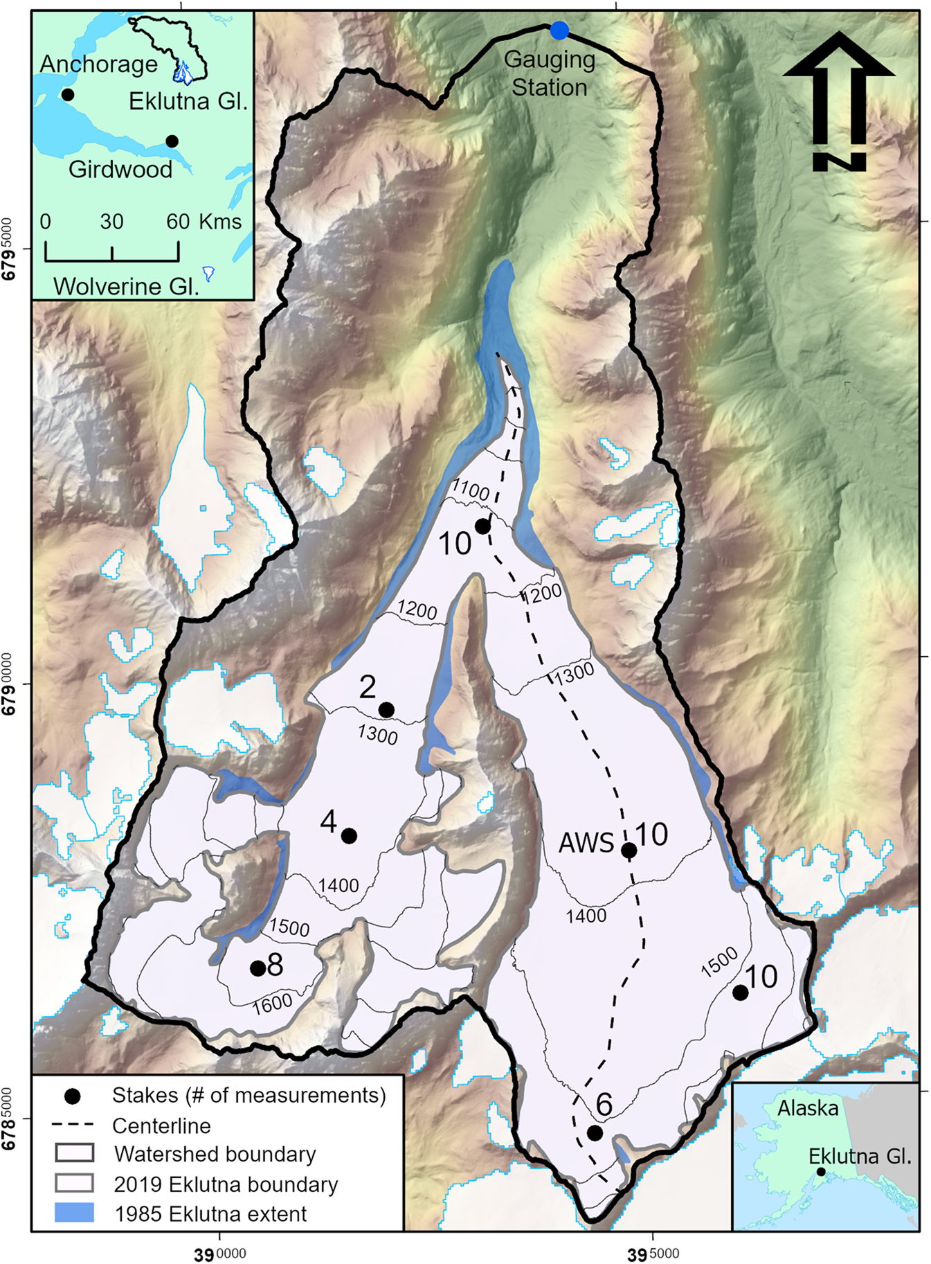
Ranging in elevation from 600 to 1700 m a.s.l., Eklutna Glacier (61.21°N, 148.98°W) is a ~29 km2 glacier located in the Western Chugach Mountains of south-central Alaska (Fig. 1). The glacier's tongue is fed by two branches: a larger main (east) branch (~16 km2) and a west branch (~13 km2). Ground-penetrating radar performed in 2010 indicated a mean ice thickness of 139 m with a maximum thickness of 430 m in the upper basin of the main branch (Sass, Reference Sass2011). The glacier is in a transitional maritime climate. An automated weather station (AWS) in coastal Girdwood (76 m a.s.l.), 25 km south of the glacier, shows a mean annual precipitation of 1907 mm from 1984 to 2014 (NOAA Cooperative Station #500243, www.wrcc.dri.edu). Measurements from an AWS operated close to the equilibrium line altitude (ELA) on the glacier from 2009 to 2015 indicate a mean melt season (May–September) air temperature of 2.2°C.
Map of Eklutna Glacier, its watershed and observation sites. The glacier area (year 2019) is shown in light grey, while the earlier 1985 extent consistent with legend is blue. Black dots represent stakes with the number of measurements over 2011–2015 calibration period. Elevation (2010) contours on glacier surface are at 100 m intervals. Black border depicts the model domain watershed. Tick marks represent easting/northing (UTM 6N, WGS84). Upper left inset map shows the location relative to Anchorage, Girdwood, Wolverine Glacier, Eklutna Glacier, and the surrounding Eklutna watershed boundary.
Eklutna Glacier has been subject to numerous research projects (Brabets, Reference Brabets1993; Larquier, Reference Larquier2011; Sass, Reference Sass2011; Sass and others, Reference Sass, Loso, Geck, Thoms and Mcgrath2017a). A field study conducted by the United States Geological Survey (USGS) for the mass-balance years 1984/85 to 1987/88 found that the annual glacier-wide mass-balance rate varied from −0.34 to 0.42 m w.e. a−1 (mean: −0.1 m w.e. a−1) and the accumulation-area ratio (AAR) ranged from 0.58 to 0.75 (mean: 0.63) (Brabets, Reference Brabets1993). For the hydrological years 1986–88, annual specific discharge (i.e. discharge per unit area of watershed area) at a gauging station (USGS 15277800 WF Eklutna) 3 km downstream from the glacier terminus ranged from 1.39 to 1.47 m (mean: 1.43 m). Alaska Pacific University has monitored both the glacier's mass balance and discharge since 2008 (Larquier, Reference Larquier2011; Sass, Reference Sass2011). Sass and others (Reference Sass, Loso and Geck2017b) found winter mass balance varied from 1.4 to 2.5 m w.e. a−1 (mean: 1.7 m w.e. a−1) and summer mass balance from −1.4 to −2.1 m w.e. a−1 (mean: −1.7 m w.e. a−1) over 2008–15.
3. Data sources and use
To model Eklutna Glacier's mass balance and discharge, a digital elevation model (DEM) of the glacier and DEM-derived slope, aspect and topographic shading, as well as climate datasets, were required. The model was forced with daily mean air temperature and precipitation observations from AWS. For calibration and validation, we used in situ surface mass-balance observations (point balances), a geodetic mass balance and snowline observations digitized from optical satellite imagery (Sass and others, Reference Sass, Loso, Geck, Thoms and Mcgrath2017a).
3.1 DEM, terrain layers and glacier boundaries
A LIDAR mission flown September 2010 with an Optech Gemini Airborne scanning system created a point-cloud with a nominal post spacing of 1.9 m and a vertical accuracy of 0.3 m (Sass and others, Reference Sass, Loso, Geck, Thoms and Mcgrath2017a). The USGS processed the point-cloud resulting in a 2.5 m gridded DEM (Sass and others, Reference Sass, Loso, Geck, Thoms and Mcgrath2017a). The DEM was used to derive surface slope, aspect, a hillshade layer, daily means of potential direct solar radiation and to delineate a watershed boundary (ArcGIS, vers. 10.6, ESRI, 2019). The hillshade layer was used to support the digitization of the 2010 glacier boundary. All layers were resampled (cubic convolution method) to a 25 m resolution for use as model input for computational efficiency while allowing spatial variations in mass balance to be captured. Glacier boundaries were manually digitized from Landsat satellite imagery for years 1985, 1993, 1999, 2006 and 2013 (Table S1). Specific years were chosen to establish a ~7-year interval over the simulation period allowing us to account for the retreat of the glacier in the simulations. Between 1985 and 2013, the glacier lost ~7% of its initial area.
3.2 Climate and weather data
Our model relies on two sources for temperature and precipitation: data from an AWS operated on the Eklutna glacier only during melt seasons (May–September) over 2011–19 and data from the nearest long-term year-round weather stations during 1984–2019. Transfer functions allowed the extension of the on-glacier temperature series to the entire period 1984–2019 for year-round model forcing.
The Eklutna Glacier AWS near the ELA (~1390 m a.s.l.) recorded hourly air temperature at 2 m above surface (Campbell Scientific, model CS215 temperature sensor) and liquid precipitation (Campbell Scientific, model TE525 tipping bucket precipitation sensor). We refer to these data as the ‘Eklutna data’.
The nearest long-term and year-round meteorological observations are from Girdwood, Alaska ~25 km south of Eklutna Glacier. We use the data from two stations as neither have a complete record of precipitation and air temperature data over the simulation period. An AWS located at the base of Alyeska Ski Resort in Girdwood recorded daily mean air temperature (76 m a.s.l., NOAA Cooperative Station #500243, www.wrcc.dri.edu) for the period October 1984–2016. A National Resource Conservation Service (NRCS) SNOTEL site also in Girdwood on Mt. Alyeska (470 m a.s.l., SNOTEL #1103, www.wcc.nrcs.usda.gov) has daily mean air temperature from 2010 to 2019. This SNOTEL site also has daily precipitation for the period October 1984–2019. We refer to the air temperature and precipitation data from the two sources as the ‘Girdwood data’.
To extend the Eklutna data temperature series (2012–19) to the entire period 1984–2019, we compared the Eklutna data to the Girdwood data to build transfer functions based on the common melt seasons of each of the Girdwood stations. An air temperature sensor failure for Eklutna data prevented the inclusion of the 2011 data observations. Since neither the NOAA nor the SNOTEL site data cover the entire period 1984–2019, we first regressed the Eklutna data against the NOAA Cooperative Station data (n = 479 days) and applied this transfer function to the NOAA Cooperative Station data 1984–2015 (Fig. 2a). Next, we regressed the Eklutna temperature data against the SNOTEL data (Fig. 2b) and applied this transfer function to the SNOTEL data for the melt seasons 2016–19. The SNOTEL daily precipitation data were used as model input without any adjustments and assumed to refer to the location (elevation) of the Eklutna AWS. Instead, biases were accounted for through a constant precipitation correction factor that was derived by model calibration (Section 2.1).
Daily mean air temperatures (°C) during the melt season (May–September) at the Eklutna AWS, T AWS, versus synthetic Eklutna temperatures, T Synthetic, derived from (a) the NOAA Cooperative Station (76 m a.s.l, 2012–2015) and (b) the SNOTEL site (470 m a.s.l., 2016–2019) in Girdwood. The synthetic data refer to temperatures after application of the transfer functions derived from regressing the measured Eklutna AWS temperatures with the NOAA and SNOTEL temperatures for the overlapping years. Transfer functions for each dataset are provided. The dashed line depicts the 1:1 line.

3.5 In situ point mass balances
Alaska Pacific University has maintained a glacier mass-balance monitoring program on both branches of Eklutna Glacier since 2008. Index sites and locations have evolved over the course of the program, with four to seven sites per year generally located near the glacier centerline and spanning the accumulation and ablation zones of each branch (Fig. 1). Point mass balances were derived at each site from measured ablation stake height, snow depth and snow pit densities (Sass and others, Reference Sass, Loso, Geck, Thoms and Mcgrath2017a, Reference Sass, Loso and Geck2017b). The sites were visited at least twice each year. In spring, snow depth was measured and snow density derived from snow pit measurements to calculate winter balances. Stakes were also installed in spring and measured again in fall to observe the summer balance. Seasonal mass balances thus refer to the floating (summer balance) and combined time system (winter balance, Cogley and others, Reference Cogley2011). For model calibration, we used observations from 2011–15, resulting in a total of 50 summer (n = 25) and winter point balances (n = 25). The point mass-balance data for the period 2011–2015 are given in Sass and others (Reference Sass, Loso, Geck, Thoms and Mcgrath2017a, Reference Sass, Loso and Geck2017b).
3.6 River discharge
River discharge was monitored on the West Fork Eklutna River ~3 km downstream from the glacier terminus. The corresponding subwatershed is 46% glacierized. A non-vented submersible pressure transducer (Onset Hobo, U20) mounted to a boulder in the river recorded the stage (water level) at hourly intervals and was verified to gage datum by standard wire-weight gage on the bridge (Rantz and others, Reference Rantz1982). Water pressures were adjusted to reflect atmospheric pressure variations (Onset Hobo, U20L) measured concurrently at the gage site. Discharge was measured by mid-section velocity measurements using a mechanical current meter (Price AA) and sounding weight (34 kg) or wading per USGS standards (Rantz and others, Reference Rantz1982). We constructed a stage–discharge relationship from 23 observations over the years 2015–19 (Fig. 3); the relationship between stage and discharge is well established for discharge <25 m3 s−1. An hourly discharge time series for the melt seasons were aggregated as daily averages to compare with model output. Historic discharge data from the USGS for 1985–1988 were also used for validation (Brabets, Reference Brabets1993; Site #15277800, https://waterdata.usgs.gov/nwis).
Stage-discharge rating curve constructed using 23 measurements (diamonds) at the watershed's gauging station (Fig. 1) of the West Fork Eklutna River for 2015–19. Dashed lines indicate ±1 sd.

3.7 Snowline position
Transient snowlines were digitized from satellite imagery over the June to September period between 1985 and 2015 (Table S1). Cloud-free satellite scenes with clearly visible snowlines were selected from Landsat 4–8 (30–60 m spatial resolution) and SPOT (5 m) as available from the USGS Earth Explorer website (earthexplorer.usgs.gov). Within a GIS (ArcGIS Ver. 10.6, ESRI, 2019), snowlines were manually digitized for each satellite melt season period scene (n = 61 snowlines; Table S1; June: 23 scenes, July: 26 scenes, August: 12 scenes). For model calibration, we created a centerline profile along the main (east) branch (Fig. 1). We then determined the centerline distance from the high point of the centerline at the glacier head to the intersection of each snowline with the centerline. This distance is used to compare modeled results with observations (henceforth referred to as snowline position). This centerline method avoids potential border effects along glacier margins from shadows, avalanche input and wind deposition. Because of difficulty discriminating snow from firn surfaces, we delineated snowlines only below the firn line (Kienholz and others, Reference Kienholz, Hock, Truffer, Bieniek and Lader2017). Field observations and late season satellite imagery allowed identification of the approximate location of the firn line. We assume a ±60 m horizontal digitizing accuracy, reflecting the coarsest satellite resolution.
4. Methods
4.1 Mass-balance and discharge model
We used the open access Distributed Enhanced Temperature Index Model (DETIM, Hock, Reference Hock1999; http://regine.github.io/meltmodel) to recreate a 35-year (1985–2019) record of surface mass balance and discharge from Eklutna Glacier. At each gridcell of the 25 m resolution DEM and at a daily time step, DETIM simulates snow accumulation, melt through a temperature index method and resulting discharge via a linear reservoir approach (Baker and others, Reference Baker, Escher-Vetter, Moser, Oerter and Reinwarth1982). Accumulation is computed from precipitation using a threshold temperature to discriminate between rain and snow. Precipitation is distributed across the glacier using a linear precipitation gradient relative to the site and elevation of the on-glacier Eklutna weather station. Melt, M (mm d−1), is calculated from daily average air temperature, T (°C), as

where f m is a melt factor (mm d−1°C−1), r ice/snow (mm m2 W−1 d−1°C−1) represents a radiation factor for snow/firn and ice surfaces, and R is the potential clear-sky direct solar radiation (W m−2).
We compute mean daily discharge from the entire watershed defined by the gauging station (i.e. including the glacier and non-glacierized areas; Fig. 1) using a linear reservoir approach (Baker and others, Reference Baker, Escher-Vetter, Moser, Oerter and Reinwarth1982). The method assumes that, at any time, t, the reservoir volume, V(t), is proportional to the reservoir discharge, Q(t)

where k is a reservoir-specific storage constant with the unit of time. Solving Eqn (2) for Q and accounting for volume changes through input to the reservoir from melt and rainwater (I), hourly discharge from the reservoir is given by:

Following Hock and Noetzli (Reference Hock and Noetzli1997), we use three linear reservoirs defined by surface type (firn, snow, ice) to account for the markedly different hydraulic properties and associated water transit velocities of these zones. The firn reservoir reflects the glacier area above a user-defined firn line which is kept constant. The snow reservoir includes any area (on or outside the glacier) with snow present at the surface but excluding the glacier firn area; the ice reservoir includes the bare ice and snow-free non-glacierized area. Ice and snow-free areas outside the glacier are treated as one single reservoir since flow velocities from ice surfaces and the generally rocky and vegetation-free non-glacierized terrain are assumed to be of similar magnitude, and we aimed to keep the number of model parameters to a minimum. On the glacier, the firn reservoir has the greatest k-value, in the order of hundreds of hours, while values for snow typically are tens of hours, and ice <30 h (Hock and others, Reference Hock, Jansson and Braun2005). K-values are obtained by calibration (Section 4.2).
For each time step, melt and rain over all catchment grid cells defining the firn, snow and ice reservoirs are summed up, and Eqn (3) is applied separately for each reservoir. Finally, each reservoir's total discharge is summed to obtain the total discharge at the location of the gauging station.
4.2 Model calibration
The mass-balance model was calibrated by optimizing six model parameters over the period 2011–15 including the temperature lapse rate (ϒ), melt factor (f m), radiation factors for ice (r ice) and snow (r snow), precipitation correction factor (p cor) and a precipitation gradient (p grad). A grid search for the best-performing mass-balance parameter combinations was applied by running the model with all parameter combinations inside a prescribed parameter space of defined increments established by preliminary testing. This resulted in a total of 257 040 model runs (Fig. 4). Each model run covered the period 1 October 2010 to 30 September 2015 (i.e. the five mass-balance years 2011–15). This period is closely aligned with the period of the geodetic mass balance reported by Sass and others (Reference Sass, Loso, Geck, Thoms and Mcgrath2017a, Reference Sass, Loso and Geck2017b) (16 September 2010–24 August 2015).
Parameter values of the 250 best-performing parameter combinations superimposed on the search parameter space. ϒ is the temperature lapse rate, f m is the melt factor, r snow and r ice are the radiation factors of ice and snow (Eqn (1)), p grad is the precipitation gradient, and p cor is the precipitation correction factor. Numbers on the left and right sides indicate the range of the parameter space and black dots mark the parameter values tested. Grey lines connect the parameter combinations of each of the 250 best-performing parameter sets. The values above each point reflect the number of successful combinations through a tested parameter (only shown if >0).

To select the best-performing parameter combinations, we first selected all parameter sets that calculated a geodetic mass balance rate that matched (within uncertainties) the 2010–2015 geodetic mass balance (−0.74 ± 0.10 m w.e. a−1) found by Sass and others (Reference Sass, Loso, Geck, Thoms and Mcgrath2017a, Reference Sass, Loso and Geck2017b). This reduced the number of potential parameter combinations to 25 062 from our original total of 257 040. Next, we performed a multi-criteria calibration by comparing the results of each remaining DETIM parameter set with both summer and winter point balance measurements and snowline positions. For each stake location, the point balance was extracted from the continuous model runs for the exact same period the measurement refers to, thus allowing direct comparability of the 50 point balances. We calibrated the model to the combined dataset of summer and winter point balances to capture the effects that melt parameters have on winter balance, for example, due to winter melt events, and precipitation parameters on summer balance, for example, due to summer snowfall events.
A total of 20 snowline positions obtained from satellite imagery were available during the calibration period (Table S1). For both variables, we quantified the agreement between modeled and observed values by calculating standard z-scores as:

where RMSEi is the root mean square error from the ith parameter set, $\overline {\rm RMSE}$ is the mean RMSE averaged across all remaining 25 062 parameter sets, and sd is the std dev of RMSE. Hence, the unitless z-score represents each parameter set's departure from the mean performance in std dev. for each variable, i.e. the point balance at index sites (in m w.e.) and distance along the glacier centerline (in m) for the snowline positions. A z-score of zero indicates an ‘average’ error; a negative z-score indicates a parameter set with less error than average, and vice versa.The z-scores of better performing parameter sets (i.e., negative z-scores) were then normalized to range between zero and one, both to allow equal weighting between variables of different units and so that larger positive values represented better fitting parameter sets than those closer to zero.
We found that a total of 7051 parameter sets (~28% of those reproducing the observed geodetic balance by Sass and others (Reference Sass, Loso, Geck, Thoms and Mcgrath2017a, Reference Sass, Loso and Geck2017b)) performed better than average for both variables. The mean z-score (±1 sd) for these 7051 parameters sets of stakes and snowline location were 0.47 ± 0.25 and 0.23 ± 0.16, respectively. For each variable, the normalized z-score maximum value of one indicates the best possible agreement between modeled and observed. Since the observations have errors and the model is overparameterized, it is not possible to determine a single best model run. Different parameter combinations can perform equally well in reproducing the observations. For example, overestimation of melt due to an overestimated degree-day factor can be compensated by an underestimated precipitation correction factor. Therefore, following previous studies (Trüssel and others, Reference Trüssel, Motyka, Truffer and Larsen2015; Kienholz and others, Reference Kienholz, Hock, Truffer, Bieniek and Lader2017), we use an ensemble of the best-performing parameter sets for further analysis and present results in terms of ensemble mean and std dev. We chose the best 250 parameter sets, thus considerably more than the ensemble of 15 and 40 best parameter sets used by Trüssel and others (Reference Trüssel, Motyka, Truffer and Larsen2015) and Kienholz and others (Reference Kienholz, Hock, Truffer, Bieniek and Lader2017), respectively.
The 250 parameter sets were chosen so that the same minimum z-score threshold was exceeded for both variables. Figure 5 demonstrates how some parameter sets perform well for point balances (high z-score) and poorly for snowlines (low z-score), and vice versa. Thus, we only retain parameter sets that yield high z-scores for both point balances and snowlines. A threshold of 0.5 yielded 250 parameter sets (Fig. 5).
Normalized z-scores for ablation stakes versus normalized z-scores of snowline positions for 7051 parameter sets. Values >0.5 for both variables (marked in red) corresponded to the 250 best-performing parameter sets. Grey lines mark the threshold of 0.5.

Figure 4 depicts the frequency of the top 250 best-performing parameter sets for the tested parameter space of each parameter. The temperature lapse rate among the best parameter sets ranged from −0.6 to −0.2°C (100 m)−1 with a mean of −0.3°C (100 m)−1 and a mode of −0.2°C (100 m)−1. All melt factors ranged from 3.75 to 6.00 mm d−1°C−1 with the most frequent values being 5.75 and 6.00 mm d−1°C−1. The radiation factor for ice was distributed across three values between 0.0242 and 0.414 m2 W−1 mm d−1°C−1 while the radiation factor for snow was most frequent in the range of 0.005 and 0.0098 m2 W−1 mm d−1°C−1. The precipitation gradient of 15% (100 m)−1 and a precipitation correction factor of 0 and 5% dominated among the best parameter sets.
In a final step, we calibrated the three storage constants k (Eqn (2)) using the 250 best-performing sets of mass-balance parameters. The coefficient does not affect the annual amounts of discharged water but modifies the seasonality of discharge by increased (higher k-values) or decreased (lower k-values) flow speed of water through the firn, snow and ice reservoirs. The k-values were determined by varying them within established ranges (Hock and others, Reference Hock, Jansson and Braun2005). Tested values for k firn, k snow and k ice ranged from 240 to 400 h (using 20 h intervals), 30–200 h (10 h intervals) and 5–25 h (1 h interval), respectively. The k-values were calibrated over 1 September 2010 to 30 August 2015 (3402 daily discharge values). A Nash–Sutcliffe model efficiency coefficient (R 2, Nash and Sutcliffe, Reference Nash and Sutcliffe1970) was calculated between modeled and observed daily discharge to assess model performance. R 2 values are typically used to assess the efficiency of hydrological model results (Krause and others, Reference Krause, Boyle and Bäse2005). Values can be negative, thus differing from the coefficient of determination r 2. These best-performing k-values (k firn = 300 h, k snow = 70 h and k ice = 15 h) were then used for all model runs.
4.3 Model validation
We cross-validated the 250 best-performing model parameter sets using (i) snowline positions, and (ii) discharge observations over periods excluded from calibration. Modeled snowline locations were compared to observations on 41 melt season days between 1985 and 2010 (Figs 6, 7). There is a tendency for the model to over-predict snow cover extent early in the season and to under-predict at the end of the season. This discrepancy may at least partially be caused by the darkening of the snow surface over the melt season, for example, through particulate and biota accumulation which is not accounted for in the model (Skiles and others, Reference Skiles, Flanner, Cook, Dumont and Painter2018). Additionally, daily mean modeled discharge was compared to observed discharge over the periods 1985–88 (Brabets, Reference Brabets1993) and 2016–19 (Fig. 7). Nash-Sutcliffe efficiency values R 2 for the hydrological years ranged from 0.66 to 0.85 (mean of best-performing 250 parameter sets) with a value of 0.77 averaged over all 8 years.
Modeled and observed snowline locations for 41 days during the melt seasons 1985–2010 for the best-performing parameter combination (ϒ = −0.2 °C (100 m)−1, M f = 5.5 mm°C−1 d−1, r ice = 0.0414 m2 W−1 mm d−1(°C)−1, r snow = 0.0098 m2 W−1 mm d−1 (°C)−1, p cor = 15% and p grad = 25% (100 m)−1). Modeled snow-covered glacier area is shown in grey, observed snowlines are depicted by blue lines, and centerline is white line. Lower right plot depicts the 41 observed (x-axis) versus modeled (y-axis) snowline positions as measured along the centerline profile (in units of 1 000 m) including the 1:1 line (grey).

Daily mean discharge during the melt seasons (May–September) for 1985–88 and 2016–19 calculated from the 250 best-performing parameter sets. The grey shading represents the range of modeled discharges with the black line representing observed discharge. Nash–Sutcliffe efficiency values (R 2) and the ratio of the modeled and observed discharge expressed in percent are provided. The blue bars reflect unaltered daily precipitation (SNOTEL #1103, www.wcc.nrcs.usda.gov). Ticks mark the first day of each month.

5. Results
5.1 Mass balance
Using the 250 best-performing mass-balance parameter sets and forcing the model with the synthetic meteorological time series derived from the observations from the Girdwood stations, we hindcast surface mass balance for the mass-balance years from 1985 to 2019 (Fig. 8). A fixed date system was applied for computing winter and summer balances with 12 May marking the end of winter and 17 September the end of summer. These dates were determined from the average annual maxima and minima of modeled cumulative mass balances (daily resolution) derived from preliminary model runs.
Modeled winter, summer and annual surface mass balance (m w.e.) for the mass-balance years 1985–2019. Results refer to mean values from the 250 best-performing parameter sets. Vertical black lines show ±1 sd (only winter and summer balances).

The mean annual surface mass balance averaged over the 250 parameter sets was −0.62 ± 0.06 m w.e. (±1 sd). The maximum annual balance (0.83 m w.e.) occurred in 1988 and the minimum (−2.3 m w.e.) in 2004 (Fig. 8). Throughout the time series, results suggest the annual surface mass balances were mostly negative. From 1985 to 2019, there is a statistically significant negative trend in annual mass balance (−0.31 m w.e. decade−1, p = 0.02; Fig. 9), due mostly to a significant negative trend in summer balance (−0.26 m w.e. decade−1, p < 0.01). No trend in winter balance was found (−0.05 m w.e. decade−1, p = 0.45).
Modeled winter (blue), summer (red) and annual (black) mass balance (m w.e.) for the mass-balance years 1985–2019. Dots show the mean of the 250 best-performing parameter sets (±1 sd) and lines show the linear trends.

Modeled glacier melt increased steadily over the near-decadal periods from 1985 to 2019 (Fig. 10). Changes in mean annual cumulative melt (hydrological year) over four consecutive 8–9-year periods (1985–93, 1994–2001, 2002–10 and 2011–19) demonstrated a 17% increase from the earliest to the latest period. In addition, the day of the year when 5 and 95% of melt have occurred is 7 days earlier in spring and 5 days later in fall in the latest period than in the earliest period, demonstrating a prolongation of the melt season. Like the near-decadal trends in annual melt, we found considerable changes over time in transient and annual AAR, computed as the ratio of snow-covered and total glacier area (Fig. 11). Annual AARs (defined by the annual AAR minima for the year) decreased from ~65% during the earliest period (1985–93) to ~45% during the latest period (2011–19). Transient AARs indicate that the glacier's winter snow cover extent is depleted faster in each consecutive period.
Modeled cumulative glacier melt between 25 April and 30 September averaged over four consecutive periods from 1985 to 2019. Cumulative melt for each year is relative to the start of the mass-balance year, i.e. 1 October of the previous calendar year. Lines give ensemble means and shading indicates ±1 sd for the 250 best-performing parameter sets. Black dots indicate when 5 and 95% of annual cumulative melt is reached. Ticks mark the first day of each month.

Modeled transient accumulation-area ratio, AAR (%) averaged over four consecutive periods between 1985 and 2019. Lines show the ensemble mean of the 250 best-performing parameter sets and shading indicates ±1 sd for the 250 best-performing parameter sets. Black dots depict the date and value of the annual AAR at the time of its minimum. Ticks mark the first day of each month.

5.2 Discharge
The modeled daily mean discharge over the melt season (May–September) increased by 17% between the 1985–1993 and the 2011–2019 interval (Figs 12, 13). The mean specific discharge averaged over the melt season period from 1985 to 2019 was 2.1 ± 0.11 m (±1 sd) with the greatest modeled specific discharge most recently (2.7 ± 0.14 m in 2019) and the lowest in 1985 (1.5 ± 0.07 m). Four of the five highest discharge years for the model period occurred after 2000 (2004, 2005, 2016 and 2019). Despite strong day-to-day variability due to differences in amount and timing of daily precipitation and melt, we find a significant trend of increasing modeled specific discharge within the melt season (0.14 m per decade, p < 0.01). Modeled melt season mean discharge represented 88 ± 3% of annual discharge over the 1985–2019 time period. The strongest increase in discharge occurred in the main melt season and fall. Summer precipitation showed no trend (p = 0.83) while temperature had an increasing trend (0.23°C per decade, p < 0.01; Fig. 12). This reinforces the notion that increasing melt dominated the discharge trend.
Mean specific discharge (a), mean air temperature (b), and total precipitation (c) during the melt season (May–September) from 1985 to 2019. Specific discharge refers to the mean of the 250 best-performing parameter sets (±1 sd). Air temperature and precipitation data reflect the data used to force the model (Section 1.5), i.e. air temperature depicts the record for the AWS site on the Eklutna Glacier extended to the entire period based on transfer functions with nearby weather stations, and precipitation refers to the nearby weather station record prior to applying the calibrated precipitation correction factor (Section 3.2). Lines show the linear trends. Vertical dotted lines mark the four averaging periods used in Figures 10, 11, 13.

Modeled daily mean discharge (m3 s−1) for the 250 best-performing parameter sets during the melt seasons (May–September) of the period 1985–2019. Four intervals are depicted: 1985–93, 1994–2001, 2002–10, 2011–19. Mean melt season precipitation for each interval is given in the legend. Shading indicates ±1 sd for the 250 best-performing parameter sets. Peaks in late fall reflect large precipitation driven flood events on 21 September 1995 and 3 October 2003. Ticks mark the first day of each month.

The entire time series was used to calculate standard hydrological metrics following Fleming and Clarke (Reference Fleming and Clarke2005), including annual median daily discharge, total annual discharge, annual maximum daily discharge and the centroid of annual hydrograph (half the year's total flow volume). Both the median daily discharge evaluated over the melt season and total annual discharge have positive significant correlations (median discharge = 0.319 × year – 57.9; p = 0.02: total annual flow = 11.8 × year – 112.77; p < 0.01). The annual maximum daily discharge and the centroid of the annual hydrograph both showed a positive trend, though not significantly correlated (max daily discharge = 0.109 × year – 191.4; p = 0.44; centroid day of year (DOY) = 0.046 × year + 114.92; p = 0.54).
6. Discussion
6.1 Model calibration
Results from model calibration indicate the value of using multi-criteria validation that includes the use of a geodetic mass-balance constraint, point balances and snowline positions. Even after a geodetic constraint, the point balances alone were not well-constrained, as the comparison between modeled and predicted point balances found 95% of individual parameter set model runs had an r 2 > 0.90 (n = 25 062). This suggests that selecting the best model parameters based solely on point balances is not sufficient. Point balances have frequently been used for melt model calibration (Hock, Reference Hock1999; Schuler and others, Reference Schuler2005), while the use of snowlines is becoming more common (Evans and others, Reference Evans, Essery and Lucas2008; Ziemen and others, Reference Ziemen2016; Kienholz and others, Reference Kienholz, Hock, Truffer, Bieniek and Lader2017; Barandun and others, Reference Barandun2018). Using only snowline observations would result in selecting different model parameter sets; however, this is expected to lead to decreased agreement between modeled and measured point mass balances as evident from Figure 5. Barandun and others (Reference Barandun2018) found the inclusion of snowlines within mass-balance modeling significantly narrowed uncertainty. Calculating a normalized z-score for each variable (point balances and snowlines) allowed equal weighting between the two variables of different units. Setting the threshold value of 0.5 allowed selecting an ensemble of 250 parameters where agreement was good for both point balances and snowlines (Fig. 4). The inclusion of both variables in addition to the geodetic balance proved necessary to provide a more robust calibration.
Model parameter values vary widely within the set of 250 best-performing parameters; however, the range in the modeled variables of the ensemble is relatively narrow for most variables (Figs 9–12). This provides confidence that the modeled trends are robust. Obviously, individual model parameter values combine to yield similar responses.
6.2 Mass balance
Eklutna Glacier mass-balance results were compared to the USGS benchmark glaciers Wolverine and Gulkana, which have been studied since the 1960s (O'Neel and others, Reference O'Neel2019). Wolverine Glacier (15.6 km2) is located within a maritime climate (Bieniek and others, Reference Bieniek2012) on the Kenai Mountains, ~90 km south of Eklutna Glacier. Gulkana Glacier (16 km2) is in a continental climate in the eastern Alaska Range, ~290 km northeast of Eklutna. The ensemble mean of the modeled annual mass balance for Eklutna Glacier is strongly correlated with the observed mass balance of Wolverine Glacier from 1985 to 2019 (r 2 = 0.73, p < 0.01, n = 35 years) and moderately correlated to the observed mass balance of Gulkana Glacier (r 2 = 0.33; p < 0.01, n = 35 years; Figs 14, 15). Some of the scatter can be attributed to the different methodologies in determining the balances including different time systems. Nevertheless, the significant correlations indicate spatially coherent climatic drivers of annual mass change. The lower correlation with Gulkana is expected given its distant location and different climatic setting. Eklutna and Wolverine glaciers are 90 km apart and each are >35 km from the Gulf of Alaska. Eklutna Glacier's annual mass balances are on average slightly higher than Wolverine. This is possibly due to Eklutna's northerly versus Wolverine's southerly orientation, and the generally cooler, somewhat transitional climate of Eklutna compared to the more maritime climate of Wolverine Glacier. While both are near the ocean, Eklutna is on the lee side of the Chugach Mountains and Wolverine on the coastal side of the Kenai Mountains.
Modeled annual mass balance (m w.e.) for Eklutna and observed balances for Wolverine and Gulkana glaciers (O'Neel and others, Reference O'Neel2019) over the period 1985–2019. Balances for Eklutna 2008–15 based on the glaciological method are also shown (Sass and others, Reference Sass, Loso, Geck, Thoms and Mcgrath2017a) correlating well with the modeled annual balances (r 2 = 0.89, p < 0.01, bias = −0.05 m w.e.).

Modeled annual mass balance (m w.e.) for Eklutna Glacier versus reported balances from (a) Wolverine Glacier and (b) Gulkana Glacier (O'Neel and others, Reference O'Neel2019) over mass-balance years 1985–2019. The grey dashed line depicts the 1:1 line.

Disagreements between modeled Eklutna and Wolverine Glacier mass-balance results in 1990 and 2009 coincide with Redoubt volcanic eruptions. Redoubt Volcano (~220 km away) erupted throughout the winter of 1989/1990 and spring of 2009 and deposited substantial amounts of volcanic ash on glacier surfaces across parts of Alaska (Waythomas and Nye, Reference Waythomas and Nye2002; Schaefer and Wallace, Reference Schaefer and Wallace2012). The largest deposit occurred in 1992 from Spurr Volcano with an estimated 500–1 000 g m−2 deposition on Eklutna Glacier and no deposition on Wolverine Glacier (McGimsey and others, Reference McGimsey, Neal and Riley2001). Such ash deposits may influence surface albedo across multiple years. DETIM as implemented here did not consider these altered surface conditions.
6.3 Discharge
The modeled increase in annual discharge over the simulation period is consistent with the negative trend in summer mass balances coincident with increasing temperatures (Fig. 12). Since summer precipitation shows no significant trend, we attribute the increase in melt season discharge to the increasingly negative glacier mass balances, and thus to the additional water released from the glacier. Changes in seasonal snow storage or precipitation over the non-glacierized catchment area may also affect the discharge trend; however, model results do not support an increase in snow accumulation outside the glacier that could have increased melt season discharge.
Results also show a lengthening of melt season (Figs 10, 13). A positive feedback may be occurring where more melt causes larger bare ice areas, exposing lower albedo ice and leading to more melt. More exposed glacier ice surface also leads to a faster throughflow of water (Hock and others, Reference Hock, Jansson and Braun2005). Hence, one can expect increases in flood peaks, especially when coincident with heavy precipitation events.
Our model results are consistent with the observations and also with other glacier discharge studies in Alaska (O'Neel and others, Reference O'Neel, Hood, Arendt and Sass2014; Beamer and others, Reference Beamer, Hill, Arendt and Liston2016). Beamer and others (Reference Beamer, Hill, Arendt and Liston2016) found glacier volume loss within the Gulf of Alaska watershed contributed 760 km3 a−1 (8%) to mean annual discharge over the period 1980–2014. O'Neel and others (Reference O'Neel, Hood, Arendt and Sass2014) found Wolverine Glacier's mass loss over the 1966–2011 period caused a 23% increase in discharge. Annual glacier discharge typically first increases as mass balances become more negative but then tends to decrease as the glacier becomes smaller (Huss and Hock, Reference Huss and Hock2018).
The positive trend in annual discharge indicates that peak water, i.e. the year when annual discharge reaches a maximum due to glacier retreat, has not been reached within the Eklutna watershed. This is consistent with the model and observational studies elsewhere in Alaska (see Hock and others (Reference Hock2019) for summary). Valentin and others (Reference Valentin, Hogue and Hay2018) project that in Eastern Alaska's Copper River watershed (60 800 km2), glacier discharge may peak in 2070 using the moderate emission scenario RCP 4.5. Global-scale projections indicate that peak water in Alaska will be reached later in the 21st century than elsewhere in the world (Huss and Hock, Reference Huss and Hock2018).
The anticipated peak water has implications for Eklutna watershed water resources. The negative mass balance currently generates water for power generation and fresh water supply above precipitation inputs; however, this surplus will decrease as glacier volume further diminishes. The earlier spring melt will provide additional water in the near term, but will not be sustainable after peak flow, as melt depletes the glacier ice reservoir. A recent study of headwater glaciers of the Columbia River found that meltwater contribution there has already reached peak flow (Moore and others, Reference Moore, Pelto, Menounos and Hutchinson2020). A future study could apply the model developed here to forecast when peak flow is reached in the Eklutna watershed under various climate change scenarios.
7. Conclusion
We calibrated the mass-balance and discharge model DETIM using a combination of geodetic and point mass-balance observations as well as snowline data. Results indicate that a multi-criteria optimization including diverse types of observations is necessary to constrain model parameters. The calibrated model allowed us to reconstruct the mass balance and glacier discharge history of Eklutna Glacier over the 35-year period 1985–2019.
Despite a wide range of model parameter values within the set of 250 best-performing model parameters, the range of the ensemble's modeled mass balance and discharge was relatively small compared to the modeled changes over time. Significant positive trends in modeled discharge are consistent with positive trends in air temperature, modeled melt season water production and prolongation of the melt season, as well as modeled negative trends in summer mass balance and AAR. The lack of significant trends in winter balance and summer precipitation suggests that the increased discharge from the highly glacierized catchment is driven by the loss of glacier mass. The modeled increase in melt season discharge throughout the simulation period indicates that peak water has not been reached. The negative trend in annual mass balance and the associated increase in discharge show that warming summers ‘mined’ the glacier’s stored water. This will have implications for water managers who seek to maximize water resources for hydropower needs as glaciers retreat and thin under a warmer climate (Hock and Jansson, Reference Hock, Jansson, Anderson and McDonnell2005). Continued monitoring of both Eklutna Glacier mass balance and discharge as model input and validation will better inform predictive models of future glacier mass and discharge as well as peak water timing.
While we found fairly good agreement between observed and predicted discharge, improvements could include the effect of variable albedos to capture the volcanic tephra deposited on Eklutna Glacier during several eruptions during the simulation period (McGimsey and others, Reference McGimsey, Neal and Riley2001; Schaefer and Wallace, Reference Schaefer and Wallace2012). Such efforts will require documenting the extent and amounts of the tephra and their impact on melt.
Supplementary material
The supplementary material for this article can be found at https://doi.org/10.1017/jog.2021.41.
Acknowledgements
S. O'Neel, H. Jiskoot, and three anonymous reviewers provided constructive criticism which led to major improvements in the manuscript. We are grateful for funding provided by NSF ARCSS (grant #1418032), National Institute for Water Resources (#2017AK137B), NASA Alaska Space Higher Education Grants and an EPSCoR RID Grant. We thank all the past students within the Alaska Pacific University (APU) Glaciology and Glacier Travel and Survey and Methods in Environmental Science field courses and other students/faculty that have helped with glacier and river fieldwork. Special thanks to past APU graduate students Ann Marie Larquier and Louis Sass. Thanks for support from the USGS Alaska Science Center, Municipal Light and Power, and Anchorage Water and Wastewater Utility. For thousands of years, the Dena'ina people have cared for this place now known as Indlu Bena (Eklutna Lake). Their sustainable and symbiotic relationships with the animals, waters and land have made this study site what it is today. These relationships are embedded in the Dena'ina language.


 Open access

