


1 INTRODUCTION
Consider the high-dimensional (HD) linear model
 $$ \begin{align} Y = X\beta + U, \end{align} $$
where the rows of the response random vector
 $Y \in \mathbb {R}^n$
are independent and identically distributed (i.i.d.) and square-integrable. The rows
$Y \in \mathbb {R}^n$
are independent and identically distributed (i.i.d.) and square-integrable. The rows
 $X_j$
,
$X_j$
,
 $1 \leq j \leq n$
, of the random covariate matrix
$1 \leq j \leq n$
, of the random covariate matrix
 $X \in \mathbb {R}^{n \times p}$
are also i.i.d. and square-integrable, with the number of observations smaller than the number of covariates (
$X \in \mathbb {R}^{n \times p}$
are also i.i.d. and square-integrable, with the number of observations smaller than the number of covariates (
 $n < p$
). Assume that
$n < p$
). Assume that
 $\mathbb {E}(X_1 U_1) = 0$
, so that the model expresses
$\mathbb {E}(X_1 U_1) = 0$
, so that the model expresses
 $Y_1$
as the sum of its projection onto the
$Y_1$
as the sum of its projection onto the
 $L_2$
space of equivalence classes of linear functions of
$L_2$
space of equivalence classes of linear functions of
 $X_1$
and an orthogonal residual
$X_1$
and an orthogonal residual
 $U_1$
.
$U_1$
.
The contribution of this article is twofold. First, we establish a new identification result showing that
 $\beta $
can be expressed as a solution to a specific generalized eigenvalue problem (GEP). Second, we leverage this result to develop a novel estimator of
$\beta $
can be expressed as a solution to a specific generalized eigenvalue problem (GEP). Second, we leverage this result to develop a novel estimator of
 $\beta $
and analyze its statistical properties.
$\beta $
and analyze its statistical properties.
GEPs involve two matrices
 $A, B \in \mathbb {R}^{p \times p}$
. Their solutions consist of scalars
$A, B \in \mathbb {R}^{p \times p}$
. Their solutions consist of scalars
 $\lambda _i$
and vectors
$\lambda _i$
and vectors
 $v_i$
that satisfy
$v_i$
that satisfy
 $$ \begin{align} A v_i = \lambda_i B v_i, \quad \text{for} \quad i = 1, \dots, p, \end{align} $$
where the
 $\lambda _i$
are called generalized eigenvalues and the
$\lambda _i$
are called generalized eigenvalues and the
 $v_i$
are the corresponding generalized eigenvectors. For a given
$v_i$
are the corresponding generalized eigenvectors. For a given
 $\lambda _i$
, the subspace spanned by all associated generalized eigenvectors is called the generalized eigenspace corresponding to
$\lambda _i$
, the subspace spanned by all associated generalized eigenvectors is called the generalized eigenspace corresponding to
 $\lambda _i$
. When B is the identity matrix, the GEP reduces to the standard eigenvalue problem (Ghojogh, Karray, and Crowley, Reference Ghojogh, Karray and Crowley2019).
$\lambda _i$
. When B is the identity matrix, the GEP reduces to the standard eigenvalue problem (Ghojogh, Karray, and Crowley, Reference Ghojogh, Karray and Crowley2019).
In Theorem 1, we show that the direction of the parameter
 $\beta $
in model (1)—that is, the subspace spanned by all vectors collinear with
$\beta $
in model (1)—that is, the subspace spanned by all vectors collinear with
 $\beta $
—is identified as the generalized eigenspace corresponding to the unique nonzero generalized eigenvalue of a pair of measurable matrices.
$\beta $
—is identified as the generalized eigenspace corresponding to the unique nonzero generalized eigenvalue of a pair of measurable matrices.
A key consequence of this identification result is that it expands the class of estimators for linear models to include those available for the GEP. As the remainder of the article shows, this is particularly advantageous in HD settings.
In HD models, the dimension of the parameter
 $\beta $
, denoted by p, exceeds the number of observations n, often because p grows with n. Estimating
$\beta $
, denoted by p, exceeds the number of observations n, often because p grows with n. Estimating
 $\beta $
in HD contexts is challenging and of significant theoretical and practical interest. The high dimensionality implies that the empirical second-moment matrix of the covariates is singular, rendering consistent estimation of
$\beta $
in HD contexts is challenging and of significant theoretical and practical interest. The high dimensionality implies that the empirical second-moment matrix of the covariates is singular, rendering consistent estimation of
 $\beta $
by ordinary least squares impossible. Nevertheless, cases with
$\beta $
by ordinary least squares impossible. Nevertheless, cases with
 $p> n$
arise frequently in fields, such as economics, finance, health studies, and machine learning (Fan and Li, Reference Fan and Li2006), motivating the development of efficient estimation methods.
$p> n$
arise frequently in fields, such as economics, finance, health studies, and machine learning (Fan and Li, Reference Fan and Li2006), motivating the development of efficient estimation methods.
There is no unique way to address the problem of consistently estimating the parameters of an HD linear model. One major line of research builds on the idea of sparsity. Box and Daniel Meyer (Reference Box and Daniel Meyer1986) originally coined the term factor sparsity to describe models in which most covariates have no effect. Since then, substantial work has focused on estimating parameters in HD sparse linear models (HDSLMs), that is, models in which only a subset of elements in
 $\beta $
are nonzero (e.g., Belloni, Chernozhukov, and Hansen, Reference Belloni, Chernozhukov and Hansen2013; van de Geer, Reference van de Geer2016). In this context, saying that a model is (exactly) sparse means that
$\beta $
are nonzero (e.g., Belloni, Chernozhukov, and Hansen, Reference Belloni, Chernozhukov and Hansen2013; van de Geer, Reference van de Geer2016). In this context, saying that a model is (exactly) sparse means that
 $$ \begin{align*} \|\beta\|_0 = s < n < p, \end{align*} $$
where s denotes the sparsity level and
 $\|v\|_0 = \sum _{i=1}^p \textbf {1}_{|v_i|> 0}$
is the
$\|v\|_0 = \sum _{i=1}^p \textbf {1}_{|v_i|> 0}$
is the
 $l_0$
-pseudonorm, which counts the number of nonzero entries in a vector.
$l_0$
-pseudonorm, which counts the number of nonzero entries in a vector.
To estimate sparse linear models, the best subset selection problem (3) arises by combining the sparsity assumption with the least squares principle:
 $$ \begin{align} \hat{\beta} \in \operatorname{\mathrm{\arg\!\min}}_{b \in \mathbb{R}^p} \frac{1}{n} \|Y - Xb\|_2^2 \quad \text{subject to} \quad \|b\|_0 \leq k, \end{align} $$
where
 $k \in \mathbb {N}$
is the maximum number of nonzero elements in b, and
$k \in \mathbb {N}$
is the maximum number of nonzero elements in b, and
 $\|v\|_2 = \left (\sum _{i=1}^p |v_i|^2\right )^{1/2}$
denotes the
$\|v\|_2 = \left (\sum _{i=1}^p |v_i|^2\right )^{1/2}$
denotes the
 $l_2$
norm of a vector v. Because of the
$l_2$
norm of a vector v. Because of the
 $l_0$
constraint, this optimization is NP-hard (Natarajan, Reference Natarajan1995), so no polynomial-time algorithm is known to solve it. Despite these computational challenges, theoretical results suggest that best subset selection remains an attractive estimator for sparse regression (e.g., Greenshtein, Reference Greenshtein2006; Raskutti, Wainwright, and Yu, Reference Raskutti, Wainwright and Yu2011; Zhang and Zhang, Reference Zhang and Zhang2012; Shen et al., Reference Shen, Pan, Zhu and Zhou2013; Zhang, Wainwright, and Jordan, Reference Zhang, Wainwright and Jordan2014; Bertsimas, King, and Mazumder, Reference Bertsimas, King and Mazumder2016). Recently, optimal or near-optimal solutions have been proposed by Bertsimas et al. (Reference Bertsimas, King and Mazumder2016), who reformulate problem (3) as a mixed integer optimization problem. Implementing this method relies on the licensed GUROBI solver and becomes increasingly demanding in computing time as the dimension of the model grows. For a critical review, see, for example, Hastie, Tibshirani, and Tibshirani (Reference Hastie, Tibshirani and Tibshirani2020).
$l_0$
constraint, this optimization is NP-hard (Natarajan, Reference Natarajan1995), so no polynomial-time algorithm is known to solve it. Despite these computational challenges, theoretical results suggest that best subset selection remains an attractive estimator for sparse regression (e.g., Greenshtein, Reference Greenshtein2006; Raskutti, Wainwright, and Yu, Reference Raskutti, Wainwright and Yu2011; Zhang and Zhang, Reference Zhang and Zhang2012; Shen et al., Reference Shen, Pan, Zhu and Zhou2013; Zhang, Wainwright, and Jordan, Reference Zhang, Wainwright and Jordan2014; Bertsimas, King, and Mazumder, Reference Bertsimas, King and Mazumder2016). Recently, optimal or near-optimal solutions have been proposed by Bertsimas et al. (Reference Bertsimas, King and Mazumder2016), who reformulate problem (3) as a mixed integer optimization problem. Implementing this method relies on the licensed GUROBI solver and becomes increasingly demanding in computing time as the dimension of the model grows. For a critical review, see, for example, Hastie, Tibshirani, and Tibshirani (Reference Hastie, Tibshirani and Tibshirani2020).
Other approaches to the best subset selection problem exist, in particular by solving a Lagrangian version of (3). However, this is not an equivalent problem because of the
 $l_0$
constraint. Within this line of research, Huang et al. (Reference Huang, Jiao, Liu and Lu2018) propose a method that, although it approximates the penalized version of (3), still allows one to fix the number of nonzero coordinates in the estimates. Hazimeh and Mazumder (Reference Hazimeh and Mazumder2020) follow a similar approach but combine the
$l_0$
constraint. Within this line of research, Huang et al. (Reference Huang, Jiao, Liu and Lu2018) propose a method that, although it approximates the penalized version of (3), still allows one to fix the number of nonzero coordinates in the estimates. Hazimeh and Mazumder (Reference Hazimeh and Mazumder2020) follow a similar approach but combine the
 $l_0$
penalty with an additional
$l_0$
penalty with an additional
 $l_q$
penalty to achieve improved algorithmic performance.
$l_q$
penalty to achieve improved algorithmic performance.
Following an approach similar to that leading to the formulation of the best subset selection, we leverage our identification result to define an estimator for the direction of
 $\beta $
under a sparsity constraint. We begin by noting that the generalized eigenvector associated with the largest generalized eigenvalue of the GEP (2) is the solution to the maximization of the following Rayleigh quotient:
$\beta $
under a sparsity constraint. We begin by noting that the generalized eigenvector associated with the largest generalized eigenvalue of the GEP (2) is the solution to the maximization of the following Rayleigh quotient:
 $$ \begin{align*} \operatorname{\mathrm{\arg\!\max}}_{v \in \mathbb{R}^p} \frac{v^\top A v}{v^\top B v}, \end{align*} $$
see, e.g., Golub and Van Loan (Reference Golub and Van Loan2013). Our identification result in Theorem 1 combines this fact with the sparsity assumption to define a sparse estimator:
 $$ \begin{align} \operatorname{\mathrm{\arg\!\max}}_{\phi \in \mathbb{R}^p} \frac{\phi^\top X^\top Y Y^\top X \phi}{n \, \phi^\top X^\top X \phi} \quad \text{subject to} \quad \|\phi\|_0 \leq k, \end{align} $$
where
 $k \in \mathbb {N}$
. We refer to (4) as the directional best subset selection problem. Our results show that for any solution of (4), say v, the product of v with the orthogonal projection of Y onto
$k \in \mathbb {N}$
. We refer to (4) as the directional best subset selection problem. Our results show that for any solution of (4), say v, the product of v with the orthogonal projection of Y onto
 $Xv$
also solves the best subset selection problem (3). Consequently, solving (4) allows us to solve (3). Furthermore, Proposition 2 below implies that both problems share the same minimax convergence rate in the
$Xv$
also solves the best subset selection problem (3). Consequently, solving (4) allows us to solve (3). Furthermore, Proposition 2 below implies that both problems share the same minimax convergence rate in the
 $l_2$
norm, specifically
$l_2$
norm, specifically
 $(s \log (p/s)/n)^{1/2}$
in the sub-Gaussian setting (Raskutti et al., Reference Raskutti, Wainwright and Yu2011).
$(s \log (p/s)/n)^{1/2}$
in the sub-Gaussian setting (Raskutti et al., Reference Raskutti, Wainwright and Yu2011).
Building on these ideas, we propose an efficient estimator for the direction of
 $\beta $
in model (1), specifically designed for HDSLMs. Our estimator is a modified version of the well-established RIFLE algorithm, originally introduced by Tan et al. (Reference Tan, Wang, Liu and Zhang2018) to approximate the solution to the GEP under an
$\beta $
in model (1), specifically designed for HDSLMs. Our estimator is a modified version of the well-established RIFLE algorithm, originally introduced by Tan et al. (Reference Tan, Wang, Liu and Zhang2018) to approximate the solution to the GEP under an
 $l_0$
constraint—an NP-hard problem (Moghaddam, Weiss, and Avidan, Reference Moghaddam, Weiss and Avidan2006)—in settings where
$l_0$
constraint—an NP-hard problem (Moghaddam, Weiss, and Avidan, Reference Moghaddam, Weiss and Avidan2006)—in settings where
 $p> n$
. We show that our estimator attains the minimax convergence rate with high probability in the sub-Gaussian setting. Finally, we establish a central limit theorem (CLT) for our estimator, addressing the nontrivial challenges arising from its nonlinearity. To do so, we prove a theorem providing sufficient conditions for the convergence in probability of a Cauchy product, which may be of independent interest.
$p> n$
. We show that our estimator attains the minimax convergence rate with high probability in the sub-Gaussian setting. Finally, we establish a central limit theorem (CLT) for our estimator, addressing the nontrivial challenges arising from its nonlinearity. To do so, we prove a theorem providing sufficient conditions for the convergence in probability of a Cauchy product, which may be of independent interest.
GEPs have previously been applied to models with many covariates. In particular, the sufficient dimension reduction framework, introduced by Dennis Cook (Reference Dennis Cook1994), uses moment-based methods that can be formulated as GEPs to replace the original covariates with a minimal set of linear combinations while preserving the relevant information (Li, Reference Li2007). Although these methods were not specifically designed for HDSLMs or for the best subset selection problem, Chen, Zou, and Cook (Reference Chen, Zou and Cook2010) proposed a method to induce sparsity in the estimated linear combinations of covariates, thereby achieving variable selection de facto.
Like the RIFLE algorithm, our estimator requires an initial solution, which it then iteratively refines until convergence. We conclude with a series of Monte Carlo experiments demonstrating the superior performance of our estimator when initialized with the Lasso method, which is the Lagrangian form of the
 $l_1$
-relaxation of problem (3) Tibshirani, Reference Tibshirani1996; Chen, Donoho, and Saunders, Reference Chen, Donoho and Saunders1998. Although the Lasso often selects an excessive number of variables when optimized for prediction accuracy Bertsimas et al., Reference Bertsimas, King and Mazumder2016; Hastie et al., Reference Hastie, Tibshirani and Tibshirani2020, our experiments show that for realistic signal-to-noise ratios (SNRs), our estimator achieves more reliable variable selection and estimation than existing
$l_1$
-relaxation of problem (3) Tibshirani, Reference Tibshirani1996; Chen, Donoho, and Saunders, Reference Chen, Donoho and Saunders1998. Although the Lasso often selects an excessive number of variables when optimized for prediction accuracy Bertsimas et al., Reference Bertsimas, King and Mazumder2016; Hastie et al., Reference Hastie, Tibshirani and Tibshirani2020, our experiments show that for realistic signal-to-noise ratios (SNRs), our estimator achieves more reliable variable selection and estimation than existing
 $l_0$
-constrained estimators.
$l_0$
-constrained estimators.
The performance of the proposed inference method, termed Loaded-RIFLE (LR), is benchmarked against three alternatives: the Lasso and two
 $l_0$
-constrained or penalized estimators. The first is the two-stage iterative hard thresholding (two-stage IHT; Jain, Tewari, and Kar, Reference Jain, Tewari, Kar, Ghahramani, Welling, Cortes, Lawrence and Weinberger2014), which extends the well-known iterative hard thresholding to approximate problem (3). The second is the support detection and root finding (SDAR) method of Huang et al. (Reference Huang, Jiao, Liu and Lu2018), which approximates the solution to the Lagrangian form of problem (3).
$l_0$
-constrained or penalized estimators. The first is the two-stage iterative hard thresholding (two-stage IHT; Jain, Tewari, and Kar, Reference Jain, Tewari, Kar, Ghahramani, Welling, Cortes, Lawrence and Weinberger2014), which extends the well-known iterative hard thresholding to approximate problem (3). The second is the support detection and root finding (SDAR) method of Huang et al. (Reference Huang, Jiao, Liu and Lu2018), which approximates the solution to the Lagrangian form of problem (3).
These existing methods have well-established minimax convergence rates and the sure screening property Jain et al., Reference Jain, Tewari, Kar, Ghahramani, Welling, Cortes, Lawrence and Weinberger2014; Huang et al., Reference Huang, Jiao, Liu and Lu2018; Guo, Zhu, and Fan, Reference Guo, Zhu and Fan2020. However, to the best of our knowledge, no CLT has yet been established for any of them.
Section 4 reports Monte Carlo experiments comparing these estimators in terms of estimation, variable selection, and prediction. Our results show that LR consistently outperforms its competitors across these metrics in many cases. In particular, LR achieves more accurate variable selection, recovering a substantial share of the true support even under low SNR conditions. Moreover, its prediction accuracy, measured by relative risk, remains robust in low-SNR regimes, highlighting its practical relevance for applications such as financial analysis, where low SNRs are common. Overall, these findings suggest that LR offers a promising alternative for reliable estimation and prediction in noisy HD settings.
The organization of the article is as follows. Section 2 establishes the identification of the direction of
 $\beta $
as the solution to a particular GEP. Section 3 builds on this result to estimate the direction of
$\beta $
as the solution to a particular GEP. Section 3 builds on this result to estimate the direction of
 $\beta $
under a sparsity assumption. We first introduce our algorithm, LR. We then provide a nonasymptotic bound on its
$\beta $
under a sparsity assumption. We first introduce our algorithm, LR. We then provide a nonasymptotic bound on its
 $l_2$
estimation error and derive its convergence rate in sub-Gaussian settings. Next, we show that this rate is minimax optimal in the sub-Gaussian case. Finally, we establish a CLT for the estimator. Section 4 presents Monte Carlo experiments that illustrate the competitiveness of LR in practice. Section 5 concludes. The Appendix collects the proofs of all results, except for the proof of the identification theorem, which is presented in Section 2. It also includes a description of the RIFLE algorithm. Technical lemmas and several standard results used throughout the proofs are provided in the Supplementary Material, where they are proved in full detail. For the convenience of the reader, a Notational Glossary is provided after the Appendix.
$l_2$
estimation error and derive its convergence rate in sub-Gaussian settings. Next, we show that this rate is minimax optimal in the sub-Gaussian case. Finally, we establish a CLT for the estimator. Section 4 presents Monte Carlo experiments that illustrate the competitiveness of LR in practice. Section 5 concludes. The Appendix collects the proofs of all results, except for the proof of the identification theorem, which is presented in Section 2. It also includes a description of the RIFLE algorithm. Technical lemmas and several standard results used throughout the proofs are provided in the Supplementary Material, where they are proved in full detail. For the convenience of the reader, a Notational Glossary is provided after the Appendix.
2 IDENTIFICATION OF THE DIRECTION OF
 $\beta $

The purpose of this section is to identify the direction of
 $\beta $
in model (1) in terms of the moments of
$\beta $
in model (1) in terms of the moments of
 $Y_1$
and
$Y_1$
and
 $X_1$
.
$X_1$
.
First, observe that in the model, since the rows of Y and X are i.i.d. in
 $L_2$
, and because
$L_2$
, and because
 $\mathbb {E}(X_1U_1)=0$
, one easily obtains normal equations
$\mathbb {E}(X_1U_1)=0$
, one easily obtains normal equations
 $\mathbb {E}(X_1Y_1)=\mathbb {E}(X_1X_1^\top )\beta $
. For every
$\mathbb {E}(X_1Y_1)=\mathbb {E}(X_1X_1^\top )\beta $
. For every
 $\beta \not \in \mathrm {Ker}(\Sigma _X):=\{v\in \mathbb {R}^p; \|\Sigma _X v\|_{2}=0\}$
, that is for every
$\beta \not \in \mathrm {Ker}(\Sigma _X):=\{v\in \mathbb {R}^p; \|\Sigma _X v\|_{2}=0\}$
, that is for every
 $\beta $
not belonging to the
$\beta $
not belonging to the
 ${kernel}$
of the second moment of
${kernel}$
of the second moment of
 $X_1$
, the latter denoted hereafter
$X_1$
, the latter denoted hereafter
 $\Sigma _X:=\mathbb {E}(X_1X_1^\top )$
, one implication of these normal equations is
$\Sigma _X:=\mathbb {E}(X_1X_1^\top )$
, one implication of these normal equations is
 $$ \begin{align*} \|\beta\|_2=\frac{\phi^\top \Sigma_{XY}}{\phi^\top \Sigma_X \phi} \end{align*} $$
with
 $\Sigma _{XY}:=\mathbb {E}(X_1Y_1)$
and
$\Sigma _{XY}:=\mathbb {E}(X_1Y_1)$
and
 $\phi :=\beta /\|\beta \|_2$
. Hence, rewriting
$\phi :=\beta /\|\beta \|_2$
. Hence, rewriting
 $\beta $
in terms of
$\beta $
in terms of
 $\phi $
and
$\phi $
and
 $\|\beta \|_2$
, one obtains after standard computations that
$\|\beta \|_2$
, one obtains after standard computations that
 $$ \begin{align} \mathbb{E}[Y_1-X_1^\top\beta]^2 &=\mathbb{E}(Y_1^2)-\frac{\phi^\top \Sigma_{XY}\Sigma_{YX}\phi}{\phi^\top \Sigma_X \phi} \end{align} $$
with
 $\Sigma _{YX}:=\Sigma _{XY}^\top $
. The condition
$\Sigma _{YX}:=\Sigma _{XY}^\top $
. The condition
 $\mathbb {E}(X_1U_1)=0$
means that
$\mathbb {E}(X_1U_1)=0$
means that
 $X_1\beta $
is the orthogonal projection of
$X_1\beta $
is the orthogonal projection of
 $Y_1$
onto the
$Y_1$
onto the
 $L^2$
subspace of linear functions of
$L^2$
subspace of linear functions of
 $X_1$
, therefore the Projection theorem (e.g., Parthasarathy, Reference Parthasarathy1977) implies that
$X_1$
, therefore the Projection theorem (e.g., Parthasarathy, Reference Parthasarathy1977) implies that
 $$ \begin{align} \beta \in \operatorname{\mathrm{\arg\!\min}}_{b\in \mathbb{R}^p} \mathbb{E}[Y_1-X_1^\top b]^2 \end{align} $$
and thus
 $$ \begin{align} \phi \in \operatorname{\mathrm{\arg\!\max}}_{b\in \mathbb{R}^p} \frac{b^\top \Sigma_{XY}\Sigma_{YX}b}{b^\top \Sigma_X b}. \end{align} $$
As appears readily, if
 $\phi $
satisfies Equation (7), so is every vector in
$\phi $
satisfies Equation (7), so is every vector in
 $\Phi =\{\alpha \beta | \alpha \in \mathbb {R}\}$
(the direction of
$\Phi =\{\alpha \beta | \alpha \in \mathbb {R}\}$
(the direction of
 $\beta $
) that is not the zero vector. Hence, the identification of
$\beta $
) that is not the zero vector. Hence, the identification of
 $\beta $
, for instance via the assumption
$\beta $
, for instance via the assumption
 $\mathrm {Ker}(\Sigma _X)=\{0\}$
, ensures the identification of
$\mathrm {Ker}(\Sigma _X)=\{0\}$
, ensures the identification of
 $\Phi $
. In contrast, the identification of
$\Phi $
. In contrast, the identification of
 $\beta $
is obtained from the identification of
$\beta $
is obtained from the identification of
 $\Phi $
by orthogonally projecting
$\Phi $
by orthogonally projecting
 $Y_1$
onto the
$Y_1$
onto the
 $L_2$
subspace of linear functions of
$L_2$
subspace of linear functions of
 $X_1^\top \phi $
for any
$X_1^\top \phi $
for any
 $\phi \in \Phi $
. This subspace is closed and convex, which ensures the uniqueness of the orthogonal projection. It is also contained in the subspace of the linear function of
$\phi \in \Phi $
. This subspace is closed and convex, which ensures the uniqueness of the orthogonal projection. It is also contained in the subspace of the linear function of
 $X_1$
. Hence, considering the orthogonal projection of
$X_1$
. Hence, considering the orthogonal projection of
 $Y_1$
as an element of this latter space uniquely identifies the solution of Equation (6), that is,
$Y_1$
as an element of this latter space uniquely identifies the solution of Equation (6), that is,
 $\beta $
in model (1).
$\beta $
in model (1).
The previous paragraph implies the following identification theorem.
Theorem 1. In model (1), assume that
 $\Sigma _X$
is positive definite, and let
$\Sigma _X$
is positive definite, and let
 $\Phi =\{\alpha \beta | \alpha \in \mathbb {R}\}$
be the direction of
$\Phi =\{\alpha \beta | \alpha \in \mathbb {R}\}$
be the direction of
 $\beta $
. Then,
$\beta $
. Then,
 $$ \begin{align} \Phi&= \mathrm{Ker}(\Sigma_{XY} \Sigma_{YX} - \Sigma_X \lambda_{\max}), \end{align} $$
where
 $\lambda _{\max }$
denotes the largest generalized eigenvalue, defined by
$\lambda _{\max }$
denotes the largest generalized eigenvalue, defined by
 $$\begin{align*}\lambda_{\max} = \max_{\phi \in \mathbb{R}^p} \frac{\phi^\top \Sigma_{XY} \Sigma_{YX} \phi}{\phi^\top \Sigma_X \phi}. \end{align*}$$
Equation (8) can be obtained by explicitly solving the maximization (7). The calculations are given in the Appendix. Hence, in this section, we have identified
 $\Phi $
as the solution set of a generalized Rayleigh quotient given in the argument of Equation (7), or equivalently, as the generalized eigenspace associated with the largest generalized eigenvalue of the matrix pair
$\Phi $
as the solution set of a generalized Rayleigh quotient given in the argument of Equation (7), or equivalently, as the generalized eigenspace associated with the largest generalized eigenvalue of the matrix pair
 $(\Sigma _{XY}\Sigma _{YX}, \Sigma _{X})$
(Equation (8)).
$(\Sigma _{XY}\Sigma _{YX}, \Sigma _{X})$
(Equation (8)).
This result highlights a general geometric property of linear models, which, to the best of our knowledge, has not been explicitly noted in the literature. However, we mention that a similar equation appears in the context of partial least squares in Sun, Ji, and Ye (Reference Sun, Ji and Ye2009).
3 ESTIMATION UNDER SPARSITY
In this section, we use the identification result of Section 2 to produce a theory of estimation of the parameter
 $\beta $
in model (1) under the assumption of sparsity. Although the literature has proposed solving specific GEPs using various least-squares formulations (e.g., Moghaddam et al., Reference Moghaddam, Weiss and Avidan2006, Sun et al., Reference Sun, Ji and Ye2009, Golub and Van Loan, Reference Golub and Van Loan2013), an original aspect of our approach is to employ a GEP to estimate the parameters of a linear model, a task typically achieved by solving least-squares problems.
$\beta $
in model (1) under the assumption of sparsity. Although the literature has proposed solving specific GEPs using various least-squares formulations (e.g., Moghaddam et al., Reference Moghaddam, Weiss and Avidan2006, Sun et al., Reference Sun, Ji and Ye2009, Golub and Van Loan, Reference Golub and Van Loan2013), an original aspect of our approach is to employ a GEP to estimate the parameters of a linear model, a task typically achieved by solving least-squares problems.
Theorem 1 suggests a directional estimation of
 $\beta $
involving two steps. First, obtain an estimation of the direction
$\beta $
involving two steps. First, obtain an estimation of the direction
 $\beta $
, say
$\beta $
, say
 $\hat {\Phi }$
, via GEP. Second, projecting Y to the span of
$\hat {\Phi }$
, via GEP. Second, projecting Y to the span of
 $X\hat {\phi }$
, for
$X\hat {\phi }$
, for
 $\hat {\phi }\in \hat {\Phi }$
and
$\hat {\phi }\in \hat {\Phi }$
and
 $\|\hat {\phi }\|_2=1$
, to obtain (say)
$\|\hat {\phi }\|_2=1$
, to obtain (say)
 $\hat {\nu }$
, an estimate of
$\hat {\nu }$
, an estimate of
 $\|\beta \|_2$
, and thus obtaining an estimator of
$\|\beta \|_2$
, and thus obtaining an estimator of
 $\beta $
by applying the Slutsky lemma to the product
$\beta $
by applying the Slutsky lemma to the product
 $\hat {\phi }\hat {\nu }$
.
$\hat {\phi }\hat {\nu }$
.
If model (1) is sparse, that is,
 $\|\beta \|_0=s<n<p$
, one may, in principle, employ the directional best subset section defined in (4) to achieve the first step of the directional estimation. As detailed in Proposition A1 in the Appendix, the solution of the best subsets selection (3) would then be exactly recovered after the second step of the procedure. Nevertheless, as stated in the Introduction, both of these problems are NP-Hard, thus, up to the time when the conjecture
$\|\beta \|_0=s<n<p$
, one may, in principle, employ the directional best subset section defined in (4) to achieve the first step of the directional estimation. As detailed in Proposition A1 in the Appendix, the solution of the best subsets selection (3) would then be exactly recovered after the second step of the procedure. Nevertheless, as stated in the Introduction, both of these problems are NP-Hard, thus, up to the time when the conjecture
 $P=NP$
has been (dis)proved, the best one can generally hope for in polynomial time is to approximate their solution. This is exactly our suggestion.
$P=NP$
has been (dis)proved, the best one can generally hope for in polynomial time is to approximate their solution. This is exactly our suggestion.
The key point relative to estimation is that Theorem 1 allows to leverage the computational ideas developed in the GEP literature to estimate
 $\beta $
in model (1). We introduce a competitive estimator based on the truncated Rayleigh flow method (called RIFLE) introduced by Tan et al. (Reference Tan, Wang, Liu and Zhang2018) to estimate the solution of GEP in HD under a sparsity constraint. This new estimator is described in Algorithm 1 below and is called Loaded-RIFLE (LR) because it is a modified version of RIFLE.
$\beta $
in model (1). We introduce a competitive estimator based on the truncated Rayleigh flow method (called RIFLE) introduced by Tan et al. (Reference Tan, Wang, Liu and Zhang2018) to estimate the solution of GEP in HD under a sparsity constraint. This new estimator is described in Algorithm 1 below and is called Loaded-RIFLE (LR) because it is a modified version of RIFLE.
Starting from an initial solution, the RIFLE as introduced by Tan et al. (Reference Tan, Wang, Liu and Zhang2018) approximates the solution of a GEP under a sparsity constraint when
 $p> n$
. The approach involves iteratively updating the estimated vector in its ascending direction, normalizing it, truncating it so that only the k coefficients with the largest absolute values remain, and then normalizing again. The resulting algorithm is detailed in the Appendix and is referred to in the main text as Algorithm 2. Our experience with RIFLE suggests that under certain conditions (specifically when the step size parameter denoted by
$p> n$
. The approach involves iteratively updating the estimated vector in its ascending direction, normalizing it, truncating it so that only the k coefficients with the largest absolute values remain, and then normalizing again. The resulting algorithm is detailed in the Appendix and is referred to in the main text as Algorithm 2. Our experience with RIFLE suggests that under certain conditions (specifically when the step size parameter denoted by
 $\eta $
is small, as expected, at least according to the theory of Tan et al. (Reference Tan, Wang, Liu and Zhang2018)), the selection of variables performed by the algorithm heavily depends on the order of the absolute values in the initial vector
$\eta $
is small, as expected, at least according to the theory of Tan et al. (Reference Tan, Wang, Liu and Zhang2018)), the selection of variables performed by the algorithm heavily depends on the order of the absolute values in the initial vector
 $\phi _0$
. In most cases, we find that this dependency limits the accuracy of the estimate. To mitigate this effect, we introduce a variant of RIFLE, that is LR.
$\phi _0$
. In most cases, we find that this dependency limits the accuracy of the estimate. To mitigate this effect, we introduce a variant of RIFLE, that is LR.
Hereafter, let
 $\hat {\Sigma }_X := X^\top X / n$
,
$\hat {\Sigma }_X := X^\top X / n$
,
 $\hat {\Sigma }_{XY} := X^\top Y / n$
, and
$\hat {\Sigma }_{XY} := X^\top Y / n$
, and
 $\hat {\Sigma }_{YX} := (\hat {\Sigma }_{XY})^\top $
serve as estimators for
$\hat {\Sigma }_{YX} := (\hat {\Sigma }_{XY})^\top $
serve as estimators for
 $\Sigma _X$
,
$\Sigma _X$
,
 $\Sigma _{XY}$
, and
$\Sigma _{XY}$
, and
 $\Sigma _{YX}$
, respectively. Moreover, for any vector
$\Sigma _{YX}$
, respectively. Moreover, for any vector
 $v \in \mathbb {R}^p$
and subset
$v \in \mathbb {R}^p$
and subset
 $\mathcal {K} \subset \{1, \dots , p\}$
, we define
$\mathcal {K} \subset \{1, \dots , p\}$
, we define
 $\text {Truncate}(v, \mathcal {K})$
as the vector in
$\text {Truncate}(v, \mathcal {K})$
as the vector in
 $\mathbb {R}^p$
given by
$\mathbb {R}^p$
given by
 $$ \begin{align*} \left(\text{Truncate}(v, \mathcal{K})\right)_i = \left\{ \begin{array}{ll} v_i, & \text{if } i \in \mathcal{K}, \\ 0, & \text{otherwise}. \end{array} \right. \end{align*} $$
Algorithm 1. Loaded and truncated Rayleigh flow method (Loaded-RIFLE).

LR can be seen as a kind of backward stepwise RIFLE. It basically runs RIFLE for
 $k=\overline {k}$
and then uses the output as input of a new run of RIFLE with
$k=\overline {k}$
and then uses the output as input of a new run of RIFLE with
 $k=\overline {k}-1$
. The algorithm proceeds as such until
$k=\overline {k}-1$
. The algorithm proceeds as such until
 $k=\underline {k}$
. The only difference lies in the IF condition in Step 4.(b)v., which ensures a somewhat smooth update of the set of selected variables. This step is important in extending the RIFLE theory developed by Tan et al. (Reference Tan, Wang, Liu and Zhang2018) to LR.
$k=\underline {k}$
. The only difference lies in the IF condition in Step 4.(b)v., which ensures a somewhat smooth update of the set of selected variables. This step is important in extending the RIFLE theory developed by Tan et al. (Reference Tan, Wang, Liu and Zhang2018) to LR.
The parameter
 $\underline {k}$
is a tuning parameter, typically expected to be larger than the true sparsity level s. In the absence of prior knowledge about s,
$\underline {k}$
is a tuning parameter, typically expected to be larger than the true sparsity level s. In the absence of prior knowledge about s,
 $\underline {k}$
can be selected using standard tuning procedures (see, e.g., Chetverikov, Reference Chetverikov2024). In the next section, we provide an example and a simulation study illustrating the effectiveness of cross-validation for this purpose.
$\underline {k}$
can be selected using standard tuning procedures (see, e.g., Chetverikov, Reference Chetverikov2024). In the next section, we provide an example and a simulation study illustrating the effectiveness of cross-validation for this purpose.
The theoretical results of the following section suggest that
 $\overline {k}$
should be chosen such that
$\overline {k}$
should be chosen such that
 $\overline {k} = Cs$
, for some sufficiently large constant C. However, since s is unknown in practice, we propose the following heuristic:
$\overline {k} = Cs$
, for some sufficiently large constant C. However, since s is unknown in practice, we propose the following heuristic:
 $\overline {k}$
should be selected to balance the computational cost and the model’s capacity to include all relevant variables. For example, when assuming the prior
$\overline {k}$
should be selected to balance the computational cost and the model’s capacity to include all relevant variables. For example, when assuming the prior
 $s \ll n < p$
, the choice
$s \ll n < p$
, the choice
 $\overline {k} \approx \frac {3}{4}n$
performs well in practice.
$\overline {k} \approx \frac {3}{4}n$
performs well in practice.
3.1 Minimax Rate of Convergence
Using techniques from Tan et al. (Reference Tan, Wang, Liu and Zhang2018) to study the convergence of RIFLE, we derive a non-asymptotic bound on the
 $l_2$
distance between the output of LR and the population target vector, defined hereafter
$l_2$
distance between the output of LR and the population target vector, defined hereafter
 $\phi ^\star :=\beta /\|\beta \|_2$
for
$\phi ^\star :=\beta /\|\beta \|_2$
for
 $\beta $
in model (1). Based on this bound, we establish the convergence rate of the estimator in a sub-Gaussian setting and demonstrate that it is minimax. Before presenting the theorems, we introduce additional notations, some of which are specific to GEP and some non-standard but useful within the context of this article.
$\beta $
in model (1). Based on this bound, we establish the convergence rate of the estimator in a sub-Gaussian setting and demonstrate that it is minimax. Before presenting the theorems, we introduce additional notations, some of which are specific to GEP and some non-standard but useful within the context of this article.
For any
 $Z\in \mathbb {R}^{p\times p}$
and
$Z\in \mathbb {R}^{p\times p}$
and
 $k\in \mathbb {N}$
s.t.
$k\in \mathbb {N}$
s.t.
 $k\leq p$
, let
$k\leq p$
, let
 $$ \begin{align*} \rho(Z,k):=\sup_{\|v\|_{2}=1, \|v\|_0\leq k} |v^\top Z v|. \end{align*} $$
For fixed k,
 $\rho (\cdot ,k):\mathbb {R}^{p\times p} \rightarrow \mathbb {R}$
is a norm on
$\rho (\cdot ,k):\mathbb {R}^{p\times p} \rightarrow \mathbb {R}$
is a norm on
 $\mathbb {R}^{p\times p}$
over
$\mathbb {R}^{p\times p}$
over
 $\mathbb {R}$
, if Z is symmetric, then
$\mathbb {R}$
, if Z is symmetric, then
 $\rho (Z,k)$
is the supremum on a set of maximum eigenvalues of submatrices of Z.
$\rho (Z,k)$
is the supremum on a set of maximum eigenvalues of submatrices of Z.
For any
 $k\in \mathbb {N}$
such that
$k\in \mathbb {N}$
such that
 $k\leq p$
let
$k\leq p$
let
 $\mathcal {F}(p,k):=\{ F\subset \{1,\ldots ,p\}; \mathrm {Card}(F)=k\}$
be the set of sets containing k different integers between
$\mathcal {F}(p,k):=\{ F\subset \{1,\ldots ,p\}; \mathrm {Card}(F)=k\}$
be the set of sets containing k different integers between
 $1$
and p. Moreover, let
$1$
and p. Moreover, let
 $\{e_i\}_{i=1}^p$
be the canonical basis in
$\{e_i\}_{i=1}^p$
be the canonical basis in
 $\mathbb {R}^p$
(i.e.,
$\mathbb {R}^p$
(i.e.,
 $e_i$
has zeros on all its elements except on the
$e_i$
has zeros on all its elements except on the
 $i^{th}$
position which contains a one) and let
$i^{th}$
position which contains a one) and let
 $\mathcal {P}\big (\mathcal {F}(p,k)\big )$
be
$\mathcal {P}\big (\mathcal {F}(p,k)\big )$
be
 $$ \begin{align*} \bigg\{P_{(F)}:=(e_{\alpha_1},\ldots,e_{\alpha_k})\in \mathbb{R}^{p\times k} \bigg| F\in \mathcal{F}(p,k); \alpha_i\in F; \alpha_1 < \alpha_2<\cdots< \alpha_k\bigg\}, \end{align*} $$
that is, the set of orthogonal projectors from
 $\mathbb {R}^p$
to its k-dimensional subspaces that are spanned by the subsets of
$\mathbb {R}^p$
to its k-dimensional subspaces that are spanned by the subsets of
 $\{e_1,\ldots ,e_p\}$
whose cardinalities equal k and that preserve the order of the indexes. This set is useful since for any
$\{e_1,\ldots ,e_p\}$
whose cardinalities equal k and that preserve the order of the indexes. This set is useful since for any
 $v\in \mathbb {R}^p$
such that
$v\in \mathbb {R}^p$
such that
 $\|v\|_0 = k$
then
$\|v\|_0 = k$
then
 $\mathcal {P}\big (\mathcal {F}(p,k)\big )$
contains a matrix P such that
$\mathcal {P}\big (\mathcal {F}(p,k)\big )$
contains a matrix P such that
 $w=P^\top v$
,
$w=P^\top v$
,
 $w\in \mathbb {R}^k$
and w is equal to v if the former is embodied in
$w\in \mathbb {R}^k$
and w is equal to v if the former is embodied in
 $\mathbb {R}^p$
. It is easy to check that any of these P satisfies
$\mathbb {R}^p$
. It is easy to check that any of these P satisfies
 $P^\top P= I_{k\times k}$
,
$P^\top P= I_{k\times k}$
,
 $\|PP^\top \|_{\mathrm {spec}}=1$
and
$\|PP^\top \|_{\mathrm {spec}}=1$
and
 $\|P\|_{\mathrm {spec}}=1$
, where for any
$\|P\|_{\mathrm {spec}}=1$
, where for any
 $Z\in \mathbb {R}^{p\times p}$
,
$Z\in \mathbb {R}^{p\times p}$
,
 $\|Z\|_{\mathrm {spec}}:= \max _{\|v\|_2=1} \|Zv\|_2$
is the spectral norm of Z.
$\|Z\|_{\mathrm {spec}}:= \max _{\|v\|_2=1} \|Zv\|_2$
is the spectral norm of Z.
For any
 $m \in \mathbb {N}$
and
$m \in \mathbb {N}$
and
 $Z\in \mathbb {R}^{m\times m}$
, let
$Z\in \mathbb {R}^{m\times m}$
, let
 $\lambda _{\mathrm {max}}(Z), \lambda _{\mathrm {min}}(Z), \text { and } \lambda _i(Z)$
be, respectively, the maximum, minimum, and
$\lambda _{\mathrm {max}}(Z), \lambda _{\mathrm {min}}(Z), \text { and } \lambda _i(Z)$
be, respectively, the maximum, minimum, and
 $i^{th}$
(in descending order) eigenvalues of Z. If Z is positive definite, let
$i^{th}$
(in descending order) eigenvalues of Z. If Z is positive definite, let
 $\kappa (Z) = \lambda _{\mathrm {max}}(Z) / \lambda _{\mathrm {min}}(Z)$
be the condition number of Z (e.g., Golub and Van Loan, Reference Golub and Van Loan2013).
$\kappa (Z) = \lambda _{\mathrm {max}}(Z) / \lambda _{\mathrm {min}}(Z)$
be the condition number of Z (e.g., Golub and Van Loan, Reference Golub and Van Loan2013).
For any
 $k\in \mathbb {N}$
s.t.
$k\in \mathbb {N}$
s.t.
 $k\leq p$
and any
$k\leq p$
and any
 $F\in \mathcal {F}(k,p)$
, let
$F\in \mathcal {F}(k,p)$
, let
 $\lambda _i$
,
$\lambda _i$
,
 $\lambda _i(F)$
,
$\lambda _i(F)$
,
 $\hat {\lambda }_i$
, and
$\hat {\lambda }_i$
, and
 $\hat {\lambda }_i(F)$
be the
$\hat {\lambda }_i(F)$
be the
 $i^{th}$
(in descending order) generalized eigenvalues of, respectively, the pairs of matrices
$i^{th}$
(in descending order) generalized eigenvalues of, respectively, the pairs of matrices
 $\big (\Sigma _{XY}\Sigma _{YX}$
,
$\big (\Sigma _{XY}\Sigma _{YX}$
,
 $\Sigma _X \big )$
,
$\Sigma _X \big )$
,
 $\big (P_{(F)}^\top \Sigma _{XY}\Sigma _{YX}P_{(F)}$
,
$\big (P_{(F)}^\top \Sigma _{XY}\Sigma _{YX}P_{(F)}$
,
 $P_{(F)}^\top \Sigma _X P_{(F)} \big )$
,
$P_{(F)}^\top \Sigma _X P_{(F)} \big )$
,
 $\big (\hat {\Sigma }_{XY}\hat {\Sigma }_{YX}$
,
$\big (\hat {\Sigma }_{XY}\hat {\Sigma }_{YX}$
,
 $\hat {\Sigma }_X\big ),$
and finally
$\hat {\Sigma }_X\big ),$
and finally
 $\big (P_{(F)}^\top \hat {\Sigma }_{XY}\hat {\Sigma }_{YX} P_{(F)}$
,
$\big (P_{(F)}^\top \hat {\Sigma }_{XY}\hat {\Sigma }_{YX} P_{(F)}$
,
 $P_{(F)}^\top \hat {\Sigma }_X P_{(F)} \big )$
.
$P_{(F)}^\top \hat {\Sigma }_X P_{(F)} \big )$
.
For any
 $p\in \mathbb {N}$
and any symmetric matrices
$p\in \mathbb {N}$
and any symmetric matrices
 $A,B \in \mathbb {R}^{p\times p}$
, let
$A,B \in \mathbb {R}^{p\times p}$
, let
 $$ \begin{align*} Cr(A,B)=\min_{\|v\|_2=1}\bigg( \big(v^\top A v\big)^2 + \big(v^\top B v )^2\bigg)^{1/2} \end{align*} $$
be the Crawford number of
 $(A,B)$
. Stewart (Reference Stewart1979) shows that if
$(A,B)$
. Stewart (Reference Stewart1979) shows that if
 $Cr(A,B)>0,$
the GEP associated with
$Cr(A,B)>0,$
the GEP associated with
 $(A,B)$
is definite, namely, it has a complete system of generalized eigenvectors and all its generalized eigenvalues are real.
$(A,B)$
is definite, namely, it has a complete system of generalized eigenvectors and all its generalized eigenvalues are real.
For any
 $k\in \mathbb {N}$
such that
$k\in \mathbb {N}$
such that
 $k\leq p$
define
$k\leq p$
define
 $$ \begin{align*} \Delta(k):= \inf_{P\in \{\cup_{i=1}^k \mathcal{P}(\mathcal{F}(p,i))\}} Cr(P^\top \Sigma_{XY}\Sigma_{YX} P, P^\top \Sigma_X P ). \end{align*} $$
and
 $$ \begin{align*} \varepsilon(k):= \bigg( \rho (\hat{\Sigma}_{XY}\hat{\Sigma}_{YX}-\Sigma_{XY}\Sigma_{YX},k)^2 + \rho(\hat{\Sigma}_X-\Sigma_X,k)^2 \bigg)^{1/2}. \end{align*} $$
In the next results, we have employed the techniques developed in Tan et al. (Reference Tan, Wang, Liu and Zhang2018) to provide a non-asymptotic bound on the
 $l_2$
error of LR.
$l_2$
error of LR.
Theorem 2. In model (1), assume
 $\Sigma _X$
is positive definite and that
$\Sigma _X$
is positive definite and that
 $\|\beta \|_0=s$
. Let
$\|\beta \|_0=s$
. Let
 $\hat {\phi }(t)$
denote the output of Algorithm 1 after t iterations of the last step,
$\hat {\phi }(t)$
denote the output of Algorithm 1 after t iterations of the last step,
 $\phi _{0}$
represent the initial truncated vector as specified in Step
$\phi _{0}$
represent the initial truncated vector as specified in Step
 $2$
of Algorithm 1 and
$2$
of Algorithm 1 and
 $\phi ^\star =\beta /\|\beta \|_2$
stand for the population target vector. Consider the following parameterization for Algorithm 1:
$\phi ^\star =\beta /\|\beta \|_2$
stand for the population target vector. Consider the following parameterization for Algorithm 1:
 $\underline {k} = C's<p$
with
$\underline {k} = C's<p$
with
 $C'> 1$
,
$C'> 1$
,
 $\overline {k} = C" \underline {k}<p-s$
with
$\overline {k} = C" \underline {k}<p-s$
with
 $C"> 1$
, and
$C"> 1$
, and
 $k' = \overline {k} + s$
. Under this parametrization, select a constant
$k' = \overline {k} + s$
. Under this parametrization, select a constant
 $c> 0$
and a step size
$c> 0$
and a step size
 $\eta $
such that
$\eta $
such that
 $$ \begin{align} \eta \lambda_{\max}(\Sigma_X) &< \frac{1}{1 + c}, \end{align} $$
 $$ \begin{align} \nu &= \left( 1 + \sqrt{\frac{s}{\underline{k}}} \right) \left( 1 - \frac{1 + c}{8} \eta \lambda_{\min}(\Sigma_X) \frac{1}{C_\diamond \kappa(\Sigma_X)} \right)^{1/2} < 1, \end{align} $$
where
 $C_\diamond = (1 + c)/(1 - c)$
. Define
$C_\diamond = (1 + c)/(1 - c)$
. Define
 $\Lambda := \lambda _{\mathrm {max}} / (1 + \lambda _{\mathrm {max}}^2)$
. Then, conditioned on the events where
$\Lambda := \lambda _{\mathrm {max}} / (1 + \lambda _{\mathrm {max}}^2)$
. Then, conditioned on the events where
 $$ \begin{align} \frac{\varepsilon(k')}{\Delta(k')} &< \frac{\Lambda(1 - \nu) \sqrt{\xi}}{4 \sqrt{10} + \Lambda(1 - \nu) \sqrt{\xi}}, \end{align} $$
 $$ \begin{align} \rho (\hat{\Sigma}_X - \Sigma_X, k') &\leq c \lambda_{\min}(\Sigma_X), \end{align} $$
 $$ \begin{align} |\langle \phi^\star, \phi_{0} \rangle_2 | &\geq 1 - \nu^2 \xi, \end{align} $$
with
 $\xi $
is defined as
$\xi $
is defined as
 $$\begin{align*}\xi := \min \left\{ \frac{1}{8 C_\diamond \kappa(\Sigma_X)}, \frac{1}{30 (1 + c) C_\diamond^3 \eta \lambda_{\max} \kappa^3(\Sigma_X)} \right\}, \end{align*}$$
the upper bound
 $$ \begin{align} \sqrt{1 - |(\phi^\star)^\top \hat{\phi}(t)|} \leq \nu^{t} \sqrt{\xi} + \frac{1}{(1 - \nu)^2} \frac{2\sqrt{5}}{\Lambda \big(\Delta(k') - \varepsilon(k')\big)} \varepsilon(k') \end{align} $$
is satisfied almost surely.
Since the theorem extends a known result from Tan et al. (Reference Tan, Wang, Liu and Zhang2018) (originally developed for RIFLE) to LR, we provide a complete proof in the Supplementary Material. This proof also fixes the proof of the theorem for RIFLE given in Tan et al. (Reference Tan, Wang, Liu and Zhang2018). (Our proof is given in the context of our article, but is readily generalizable to the setup of Tan et al. (Reference Tan, Wang, Liu and Zhang2018).)
Theorem 2 enables us to bound the
 $l_2$
norm between
$l_2$
norm between
 $\phi ^\star $
and
$\phi ^\star $
and
 $\hat {\phi }(t)$
. Specifically, when the inner product
$\hat {\phi }(t)$
. Specifically, when the inner product
 $\langle \phi ^\star , \hat {\phi }(t) \rangle _2 \geq 0$
, we have
$\langle \phi ^\star , \hat {\phi }(t) \rangle _2 \geq 0$
, we have
 $\sqrt {1 - |(\phi ^\star )^\top \hat {\phi }(t)|} = 1/\sqrt {2} \|\phi ^\star - \hat {\phi }(t)\|_2$
.
$\sqrt {1 - |(\phi ^\star )^\top \hat {\phi }(t)|} = 1/\sqrt {2} \|\phi ^\star - \hat {\phi }(t)\|_2$
.
The first term on the right-hand side,
 $\nu ^{t} \sqrt {\xi }$
, represents the optimization error, while the second term represents the statistical error (Tan et al., Reference Tan, Wang, Liu and Zhang2018).
$\nu ^{t} \sqrt {\xi }$
, represents the optimization error, while the second term represents the statistical error (Tan et al., Reference Tan, Wang, Liu and Zhang2018).
Assumptions (11) and (12) control the estimation error for the (generalized) spectrum of the matrix pair. Specifically, these assumptions provide bounds on the condition number of
 $\Sigma _X$
, on the spectra of submatrices of
$\Sigma _X$
, on the spectra of submatrices of
 $\hat {\Sigma }_X$
, and on
$\hat {\Sigma }_X$
, and on
 $\hat {\lambda }_i(F)$
for any
$\hat {\lambda }_i(F)$
for any
 $F \in \mathcal {F}(p, k')$
and
$F \in \mathcal {F}(p, k')$
and
 $i = 1, \dots , k'$
; details can be found in Tan et al. (Reference Tan, Wang, Liu and Zhang2018). As shown later, if
$i = 1, \dots , k'$
; details can be found in Tan et al. (Reference Tan, Wang, Liu and Zhang2018). As shown later, if
 $Y_1$
and
$Y_1$
and
 $X_1$
are sub-Gaussian, there exist ratios among n,
$X_1$
are sub-Gaussian, there exist ratios among n,
 $p(n)$
, and
$p(n)$
, and
 $s(n)$
such that the probability of events where these assumptions fail converges to zero as
$s(n)$
such that the probability of events where these assumptions fail converges to zero as
 $n \rightarrow \infty $
.
$n \rightarrow \infty $
.
Theorem 2 also requires certain theoretical conditions on the input parameters of Algorithm 1.
Inequalities (9) and (10) impose technical restrictions on step size
 $\eta $
. Currently, there is no known method to select
$\eta $
. Currently, there is no known method to select
 $\eta $
that consistently meets these theoretical criteria. However, both experience and Assumption (9) from Tan et al. (Reference Tan, Wang, Liu and Zhang2018) suggest selecting
$\eta $
that consistently meets these theoretical criteria. However, both experience and Assumption (9) from Tan et al. (Reference Tan, Wang, Liu and Zhang2018) suggest selecting
 $\eta $
small enough to satisfy
$\eta $
small enough to satisfy
 $\eta \lambda (\hat {\Sigma }_X) < 1$
.
$\eta \lambda (\hat {\Sigma }_X) < 1$
.
Furthermore, Equation (13) requires that the cosine between the target vector (population)
 $\phi ^\star $
and the input vector
$\phi ^\star $
and the input vector
 $\phi _0$
be sufficiently large. We discuss the choice of the initial vector in the following result and example. This result gives an explicit convergence rate depending on the initialization of Algorithm 1. The next example shows how this result applies in practice.
$\phi _0$
be sufficiently large. We discuss the choice of the initial vector in the following result and example. This result gives an explicit convergence rate depending on the initialization of Algorithm 1. The next example shows how this result applies in practice.
Proposition 1. In model (1) assume that
 $Y_1$
,
$Y_1$
,
 $X_{1,1}, \dots , X_{1,p(n)}$
are sub-Gaussian, that
$X_{1,1}, \dots , X_{1,p(n)}$
are sub-Gaussian, that
 $\Sigma _X := \mathbb {E}(X_1 X_1^\top )$
is positive definite and that
$\Sigma _X := \mathbb {E}(X_1 X_1^\top )$
is positive definite and that
 $\|\beta \|_0 = s$
. Let
$\|\beta \|_0 = s$
. Let
 $\hat {\phi }(t)$
denote the output of Algorithm 1 after t iterations in the last step. Let
$\hat {\phi }(t)$
denote the output of Algorithm 1 after t iterations in the last step. Let
 $\phi _{0}$
be the initial truncated vector as specified in Step
$\phi _{0}$
be the initial truncated vector as specified in Step
 $2$
of Algorithm 1 and
$2$
of Algorithm 1 and
 $\phi ^\star =\beta /\|\beta \|_2$
represent the population target vector. Suppose that
$\phi ^\star =\beta /\|\beta \|_2$
represent the population target vector. Suppose that
 $\langle \phi ^\star , \hat {\phi }(t) \rangle _2 \geq 0$
a.s. and that
$\langle \phi ^\star , \hat {\phi }(t) \rangle _2 \geq 0$
a.s. and that
 $s\log (p/s)/n=o(1)$
and
$s\log (p/s)/n=o(1)$
and
 $s/p=o(1)$
. Then, under assumptions (9) and (10) of Theorem 2 if
$s/p=o(1)$
. Then, under assumptions (9) and (10) of Theorem 2 if
 $$\begin{align*}\|\phi^\star - \phi_{0}\|_2 = O_p(\alpha_n) \end{align*}$$
with
 $\alpha _n = o(1)$
, then there exists a choice of
$\alpha _n = o(1)$
, then there exists a choice of
 $t = t(n)$
such that
$t = t(n)$
such that
 $$\begin{align*}\|\phi^\star - \hat{\phi}(t)\|_2 = O_p \left( \sqrt{\frac{s \log(p/s)}{n}} \right). \end{align*}$$
The proof is given in the Appendix. An estimate of the magnitude of
 $\beta $
can then be obtained by regressing Y onto the span of
$\beta $
can then be obtained by regressing Y onto the span of
 $X\hat {\phi }(t)$
. Let
$X\hat {\phi }(t)$
. Let
 $\hat {\upsilon }$
be this estimator, and let
$\hat {\upsilon }$
be this estimator, and let
 $\hat {\beta }$
denote the estimator of
$\hat {\beta }$
denote the estimator of
 $\beta $
obtained as the product of
$\beta $
obtained as the product of
 $\hat {\phi }(t)$
and
$\hat {\phi }(t)$
and
 $\hat {\upsilon }$
. Proposition 2 below tells us that for
$\hat {\upsilon }$
. Proposition 2 below tells us that for
 $t = t(n)$
growing sufficiently fast, we have
$t = t(n)$
growing sufficiently fast, we have
 $\|\hat {\beta } - \beta \|_2 = O_p\big ((s \log (p / s) / n)^{1/2}\big )$
, which is minimax (Raskutti et al., Reference Raskutti, Wainwright and Yu2011).
$\|\hat {\beta } - \beta \|_2 = O_p\big ((s \log (p / s) / n)^{1/2}\big )$
, which is minimax (Raskutti et al., Reference Raskutti, Wainwright and Yu2011).
Example 1 [Loaded-RIFLE-post-Lasso].
To obtain a reliable initial vector, one might follow the heuristic suggested in Tan et al. (Reference Tan, Wang, Liu and Zhang2018) by using a solution from an
 $l_1$
relaxation of the
$l_1$
relaxation of the
 $l_0$
constrained problem as the initial vector, specifically the Lasso solution for the problem (3) Bertsimas et al., Reference Bertsimas, King and Mazumder2016; Hastie et al., Reference Hastie, Tibshirani and Tibshirani2020.
$l_0$
constrained problem as the initial vector, specifically the Lasso solution for the problem (3) Bertsimas et al., Reference Bertsimas, King and Mazumder2016; Hastie et al., Reference Hastie, Tibshirani and Tibshirani2020.
This choice of initialization is particularly suitable since the Lasso is known to select a large number of covariates when optimized for predictive accuracy. Using its (normalized) solution as the initial vector for Algorithm 1 enables us to reduce the size of the selected support while improving the accuracy of the estimation. As demonstrated in the Monte Carlo experiments in Section 5, this procedure outperforms the other
 $l_0$
-constrained estimators considered in this article.
$l_0$
-constrained estimators considered in this article.
The theoretical validity of this initialization procedure depends on how the Lasso is tuned. For example, Chetverikov, Liao, and Chernozhukov (Reference Chetverikov, Liao and Chernozhukov2021) established that the
 $l_2$
error of cross-validated Lasso is
$l_2$
error of cross-validated Lasso is
 $O_p\big ((s \log (p/s) / n)^{1/2} \times \log (pn)\big )$
. This error rate ensures that the probability of events where the assumptions on
$O_p\big ((s \log (p/s) / n)^{1/2} \times \log (pn)\big )$
. This error rate ensures that the probability of events where the assumptions on
 $\phi _0$
in Theorem 2 are violated converges to zero. Other tuning methods for the Lasso that provide similar guarantees are available. For example, one alternative to cross-validation could be to set the penalty parameter based on the self-normalized moderate deviation theory, as proposed in Belloni et al. (Reference Belloni, Chen, Chernozhukov and Hansen2012).
$\phi _0$
in Theorem 2 are violated converges to zero. Other tuning methods for the Lasso that provide similar guarantees are available. For example, one alternative to cross-validation could be to set the penalty parameter based on the self-normalized moderate deviation theory, as proposed in Belloni et al. (Reference Belloni, Chen, Chernozhukov and Hansen2012).
To finalize the theoretical analysis of the convergence of LR, we demonstrate that the convergence rate obtained in Proposition 1 in the sub-Gaussian setting is actually optimal, in the sense that it is the minimax convergence rate of the selection of the directional best subset selection defined by Equation (4). To demonstrate this statement, the following proposition connects the estimation error of
 $\beta $
in the model (1) under the assumption of sparsity to the estimation error of
$\beta $
in the model (1) under the assumption of sparsity to the estimation error of
 $\phi ^\star $
, thus linking the minimax convergence rates of the two estimators.
$\phi ^\star $
, thus linking the minimax convergence rates of the two estimators.
Proposition 2. In model (1) suppose that
 $\Sigma _X := \mathbb {E}(X_1 X_1^\top )$
is positive definite and that
$\Sigma _X := \mathbb {E}(X_1 X_1^\top )$
is positive definite and that
 $\|\beta \|_0 = s$
. Let
$\|\beta \|_0 = s$
. Let
 $\hat {\phi } \in \mathbb {R}^p$
be an estimator of
$\hat {\phi } \in \mathbb {R}^p$
be an estimator of
 $\phi ^\star :=\beta /\|\beta \|_2$
that satisfies the following conditions a.s.:
$\phi ^\star :=\beta /\|\beta \|_2$
that satisfies the following conditions a.s.:
 $$\begin{align*}\langle \hat{\phi}, \phi^\star \rangle_2 \geq 0, \quad \|\hat{\phi}\|_2 = 1, \quad \|\hat{\phi}\|_0 = Cs \text{ with }C\geq 1, \end{align*}$$
the convergence rate
 $\|\hat {\phi } - \phi ^\star \|_2 = O_p(\alpha _n)$
, where
$\|\hat {\phi } - \phi ^\star \|_2 = O_p(\alpha _n)$
, where
 $\alpha _n = o(1)$
and
$\alpha _n = o(1)$
and
 $(2s / n)^{1/2} / \alpha _n = o(1)$
, and let
$(2s / n)^{1/2} / \alpha _n = o(1)$
, and let
 $\hat {\upsilon } = \operatorname {\mathrm {\arg \!\min }}_{m \in \mathbb {R}} \|Y - X \hat {\phi } m\|_2^2$
be an estimator of
$\hat {\upsilon } = \operatorname {\mathrm {\arg \!\min }}_{m \in \mathbb {R}} \|Y - X \hat {\phi } m\|_2^2$
be an estimator of
 $\|\beta \|_2$
. Assume that there exist constants
$\|\beta \|_2$
. Assume that there exist constants
 $0 < \underline {\kappa } \leq \overline {\kappa } < \infty $
such that, for all
$0 < \underline {\kappa } \leq \overline {\kappa } < \infty $
such that, for all
 $u \in \mathbb {R}^p$
with
$u \in \mathbb {R}^p$
with
 $\|u\|_2 = 1$
and
$\|u\|_2 = 1$
and
 $\|u\|_0 = \min \{2s, p\}$
, the inequality
$\|u\|_0 = \min \{2s, p\}$
, the inequality
 $$ \begin{align} \underline{\kappa} \leq u^\top \hat{\Sigma}_X u \leq \overline{\kappa} \end{align} $$
holds true almost surely. Then, if
 $\hat {\beta } \in \mathbb {R}^p$
is an estimator of
$\hat {\beta } \in \mathbb {R}^p$
is an estimator of
 $\beta $
satisfying
$\beta $
satisfying
 $\hat {\beta } = \hat {\phi } \hat {\upsilon }$
a.s., we have
$\hat {\beta } = \hat {\phi } \hat {\upsilon }$
a.s., we have
 $$\begin{align*}\|\hat{\beta} - \beta \|_2^2 = c \|\hat{\phi} - \phi^\star\|_2^2 + O_p\big(\alpha_n^2\big) \hspace{5mm} \text{ a.s.}, \end{align*}$$
where
 $c = O_p(1)$
.
$c = O_p(1)$
.
The proof is given in the Appendix. The proposition provides sufficient conditions to ensure that the
 $l_2$
convergence rate of
$l_2$
convergence rate of
 $\hat {\beta }$
is dominated by the
$\hat {\beta }$
is dominated by the
 $l_2$
convergences of the direction estimator
$l_2$
convergences of the direction estimator
 $\hat {\phi }$
.
$\hat {\phi }$
.
This result is important because it implies that the minimax convergence rate in the loss
 $l_2$
of the directional best subset selection (4) is the same as that of the best subset selection (3). Raskutti et al. (Reference Raskutti, Wainwright and Yu2011) have proven that in a Gaussian fixed design (that is, restricting oneself to an analysis conditionally on X), if a version of assumption (15) holds, the minimax convergence rate of
$l_2$
of the directional best subset selection (4) is the same as that of the best subset selection (3). Raskutti et al. (Reference Raskutti, Wainwright and Yu2011) have proven that in a Gaussian fixed design (that is, restricting oneself to an analysis conditionally on X), if a version of assumption (15) holds, the minimax convergence rate of
 $\|\hat {\beta }-\beta \|_2$
is
$\|\hat {\beta }-\beta \|_2$
is
 $(s\log (p/s)/n)^{1/2}$
(since
$(s\log (p/s)/n)^{1/2}$
(since
 $\hat {\beta }$
is the best selection of subsets). Given that this rate is obtained in fixed design, it is actually a lower bound on the unconditioned convergence of the best subset selection defined in Equation (3), and thus by Proposition 2 of the directional best subset selection in (4). Since by Proposition 1, LR actually achieves this rate in the sub-Gaussian, unconditioned setting, it must be that the rate obtained in Raskutti et al. (Reference Raskutti, Wainwright and Yu2011) is actually the minimax rate of convergence of the directional best subset selection, thus concluding the demonstration of our claim of optimality of LR.
$\hat {\beta }$
is the best selection of subsets). Given that this rate is obtained in fixed design, it is actually a lower bound on the unconditioned convergence of the best subset selection defined in Equation (3), and thus by Proposition 2 of the directional best subset selection in (4). Since by Proposition 1, LR actually achieves this rate in the sub-Gaussian, unconditioned setting, it must be that the rate obtained in Raskutti et al. (Reference Raskutti, Wainwright and Yu2011) is actually the minimax rate of convergence of the directional best subset selection, thus concluding the demonstration of our claim of optimality of LR.
3.2 Central Limit Theorem
In this section, we establish a CLT for the output of LR. Before presenting the results, we introduce the following definition, which is essential for the statement and proof of the theorem.
Definition 1. In model (1), let
 $\phi ^\star :=\beta /\|\beta \|_2$
as above, and
$\phi ^\star :=\beta /\|\beta \|_2$
as above, and
 $\|\beta \|_0<k\in \mathbb {N}$
. Hereafter, we reserve the notation
$\|\beta \|_0<k\in \mathbb {N}$
. Hereafter, we reserve the notation
 $\mathcal {Q}^\star $
for the set of matrices defined by
$\mathcal {Q}^\star $
for the set of matrices defined by
 $$ \begin{align*} \mathcal{Q}^\star:=\{Q=PP^\top | P\in \cup_{i=\|\phi\|_0}^k \mathcal{P}\big(\mathcal{F}(p,i)\big), Q\phi^\star=\phi^\star\}. \end{align*} $$
Moreover, hereafter, we define for any output of Algorithm 2 noted
 $\hat {\phi }(t)$
 $$ \begin{align*} Q\big(\hat{\phi}(t)\big)=Q_t=P_tP_t^\top, \end{align*} $$
where
 $P_t$
is the element of
$P_t$
is the element of
 $\mathcal {P}(\mathcal {F}(p,\|\hat {\phi }(t)\|_0))$
that is such that if
$\mathcal {P}(\mathcal {F}(p,\|\hat {\phi }(t)\|_0))$
that is such that if
 $w= P_t^\top \hat {\phi }(t),$
then w is equal to
$w= P_t^\top \hat {\phi }(t),$
then w is equal to
 $\hat {\phi }(t)$
if the former is embodied in
$\hat {\phi }(t)$
if the former is embodied in
 $\mathbb {R}^p$
.
$\mathbb {R}^p$
.
We note that any output of Algorithm 1, say
 $\hat {\phi }(t)$
, that is such that
$\hat {\phi }(t)$
, that is such that
 $Q\big (\hat {\phi }(t)\big )\in \mathcal {Q}^\star $
, has a support containing the support of
$Q\big (\hat {\phi }(t)\big )\in \mathcal {Q}^\star $
, has a support containing the support of
 $\phi ^{\star }$
. From Lemma A5 in the Appendix, one can show that in the sub-Gaussian setting, for
$\phi ^{\star }$
. From Lemma A5 in the Appendix, one can show that in the sub-Gaussian setting, for
 $t=t(n)$
fast enough,
$t=t(n)$
fast enough,
 $Q\big (\hat {\phi }(t)\big )\in \mathcal {Q}^\star $
with probability tending to one, i.e., LR possesses sure screening property Fan and Lv, Reference Fan and Lv2008; Guo et al., Reference Guo, Zhu and Fan2020.
$Q\big (\hat {\phi }(t)\big )\in \mathcal {Q}^\star $
with probability tending to one, i.e., LR possesses sure screening property Fan and Lv, Reference Fan and Lv2008; Guo et al., Reference Guo, Zhu and Fan2020.
In the following, we make use of the following convention.
Notation 1. Let
 $\{a_\alpha \}_{\alpha \in \mathbb {N}}$
be a family of operators in a vector space, if
$\{a_\alpha \}_{\alpha \in \mathbb {N}}$
be a family of operators in a vector space, if
 $j<i,$
then
$j<i,$
then
 $\prod _{\alpha =i}^j a_\alpha =1$
. where in the above expression,
$\prod _{\alpha =i}^j a_\alpha =1$
. where in the above expression,
 $1$
represents the unitary operator in the vector space. If
$1$
represents the unitary operator in the vector space. If
 $j \geq i,$
the symbol
$j \geq i,$
the symbol
 $\prod $
is used conventionally.
$\prod $
is used conventionally.
We now state the CLT for the output of Algorithm 1.
Theorem 3. In model (1), suppose that
 $ \Sigma _X := \mathbb {E}(X_1 X_1^\top ) $
is positive definite and
$ \Sigma _X := \mathbb {E}(X_1 X_1^\top ) $
is positive definite and
 $ \|\beta \|_0=s $
.
$ \|\beta \|_0=s $
.
Let
 $ \sigma ^2 = \operatorname {Var}(U_1) $
,
$ \sigma ^2 = \operatorname {Var}(U_1) $
,
 $ \phi ^\star := \beta / \|\beta \|_{2} $
and
$ \phi ^\star := \beta / \|\beta \|_{2} $
and
 $\hat {\phi }(t)$
be the output of Algorithm 1 after t iteration of the last step. Moreover, let
$\hat {\phi }(t)$
be the output of Algorithm 1 after t iteration of the last step. Moreover, let
 $\eta, \phi_{t-1} $
and
$\eta, \phi_{t-1} $
and
 $ C_{t-1} $
be as in Algorithm 2 and let
$ C_{t-1} $
be as in Algorithm 2 and let
 $ \tilde {\phi _t} := C_{t-1} \phi _{t-1} $
. Assume
$ \tilde {\phi _t} := C_{t-1} \phi _{t-1} $
. Assume
 $ t $
is an increasing function of
$ t $
is an increasing function of
 $ n $
and that
$ n $
and that
 $ \langle \phi ^\star , \hat {\phi }(t) \rangle _2 \geq 0 $
holds almost surely.
$ \langle \phi ^\star , \hat {\phi }(t) \rangle _2 \geq 0 $
holds almost surely.
Suppose there exist constants
 $ \xi> 0 $
and
$ \xi> 0 $
and
 $ \nu < 1 $
such that
$ \nu < 1 $
such that
 $$ \begin{align} \|\phi^\star - \hat{\phi}(t)\|_2 &\leq \nu^t \sqrt{\xi} + O_p\bigg(\sqrt{\frac{s \log(p/s)}{n}}\bigg), \end{align} $$
and that
 $ \inf _{\|v\|_{2} = 1, \|v\|_0 = k} |v^\top \Sigma _{XY}|> 0 $
with
$ \inf _{\|v\|_{2} = 1, \|v\|_0 = k} |v^\top \Sigma _{XY}|> 0 $
with
 $ \log (n)/t(n) = o(1) $
.
$ \log (n)/t(n) = o(1) $
.
Then, conditionally on
 $ X $
, there exists a matrix
$ X $
, there exists a matrix
 $ Q^\star \in \mathcal {Q}^\star $
and a constant
$ Q^\star \in \mathcal {Q}^\star $
and a constant
 $ K> 0 $
such that if
$ K> 0 $
such that if
 $ \eta < K $
, then for any unit vector
$ \eta < K $
, then for any unit vector
 $ w \in \mathbb {R}^p, \|w\|_0 \leq \|\hat {\phi }(t)\|_0 $
, we have
$ w \in \mathbb {R}^p, \|w\|_0 \leq \|\hat {\phi }(t)\|_0 $
, we have
 $$\begin{align*}\sqrt{n} \langle w, \hat{\phi}(t) - \phi^\star + \gamma_n \rangle_{2} \end{align*}$$
is asymptotically normal,
 $$\begin{align*}\mathcal{AN}\left( 0, w^\top [(I - Q^\star) + \eta \hat{\Sigma}_X Q^\star]^{-1} \eta^2 \hat{\Sigma}_X[(I - Q^\star) + \eta \hat{\Sigma}_X Q^\star]^{-1} w \frac{\sigma^2}{\|\beta\|_{2}^2} \bigg| X \right), \end{align*}$$
with
 $ \|\gamma _n\|_2 = o_p(1) $
, where
$ \|\gamma _n\|_2 = o_p(1) $
, where
 $ \gamma _n := \kappa _n + \tau _n $
.
$ \gamma _n := \kappa _n + \tau _n $
.
Here,
 $$\begin{align*}\kappa_n = \sum_{m=0}^{t-1} \left( \prod_{l=1}^m (I_{p \times p} - \eta \hat{\Sigma}_X) Q_{t-l} \right)(\phi_{t-l} - \tilde{\phi}_{t-l}), \end{align*}$$
and
 $$\begin{align*}\tau_n = \left[ \sum_{m=0}^{t-1} \left( \prod_{l=1}^m (I_{p \times p} - \eta \hat{\Sigma}_X) Q_{t-l} g_{t-1-m} \right) \big( (I - Q^{\star}) + \eta \hat{\Sigma}_X Q^{\star} \big) - I_{p \times p} \right] \phi^\star, \end{align*}$$
with
 $$\begin{align*}g_{t-1-m} = \frac{\phi_{t-1-m}^\top \hat{\Sigma}_X \phi_{t-1-m}}{\phi_{t-1-m}^\top \hat{\Sigma}_X \phi^\star + \phi_{t-1-m}^\top \frac{X^\top U}{\|\beta\|_{2} n}}. \end{align*}$$
The proof of this result is provided in the Appendix. The bias term
 $\gamma _n$
consists of two parts:
$\gamma _n$
consists of two parts:
 $\kappa _n$
, which is observable (and therefore correctable), and
$\kappa _n$
, which is observable (and therefore correctable), and
 $\tau _n$
, which is unobservable. In the proof, we show that both terms converge to zero, although we cannot determine their exact rates of convergence. From Assumption (16) (which can be verified in the sub-Gaussian, see Proposition 1), we conclude that
$\tau _n$
, which is unobservable. In the proof, we show that both terms converge to zero, although we cannot determine their exact rates of convergence. From Assumption (16) (which can be verified in the sub-Gaussian, see Proposition 1), we conclude that
 $\gamma _n$
converges to zero at a slower rate than
$\gamma _n$
converges to zero at a slower rate than
 $n^{-1/2}$
.
$n^{-1/2}$
.
The term
 $\kappa _n$
accounts for the effects of normalization in Step 3.c) and truncation in Step 3.e) of Algorithm 2. The term
$\kappa _n$
accounts for the effects of normalization in Step 3.c) and truncation in Step 3.e) of Algorithm 2. The term
 $\tau _n$
arises primarily from the difference in supports between
$\tau _n$
arises primarily from the difference in supports between
 $\hat {\phi }(t)$
and
$\hat {\phi }(t)$
and
 $\phi ^\star $
and can be seen as a bias introduced by regularizing the inverse problem posed by the ill-conditioned matrix
$\phi ^\star $
and can be seen as a bias introduced by regularizing the inverse problem posed by the ill-conditioned matrix
 $\hat {\Sigma }_X$
when estimating
$\hat {\Sigma }_X$
when estimating
 $\phi ^\star $
in HD settings.
$\phi ^\star $
in HD settings.
The proof of Theorem 3 is based on three propositions: Propositions A3–A5 stated and proved in the Appendix. Proposition A3 provides conditions for the convergence in probability of a stochastic Cauchy product and may be of independent interest. Propositions A4 and A5 analyze LR in depth and are also discussed in the Appendix.
4 MONTE CARLO EXPERIMENTS
The performances of LR are compared against the cross-validated Lasso, as well as two well-studied
 $l_0$
-constrained estimators of
$l_0$
-constrained estimators of
 $\beta $
: the SDAR (Huang et al., Reference Huang, Jiao, Liu and Lu2018) and the two-stage IHT (Jain et al., Reference Jain, Tewari, Kar, Ghahramani, Welling, Cortes, Lawrence and Weinberger2014).
$\beta $
: the SDAR (Huang et al., Reference Huang, Jiao, Liu and Lu2018) and the two-stage IHT (Jain et al., Reference Jain, Tewari, Kar, Ghahramani, Welling, Cortes, Lawrence and Weinberger2014).
4.1 Setup
The following experiment is reproduced
 $100$
times. In each experiment, we set
$100$
times. In each experiment, we set
 $n = 100$
,
$n = 100$
,
 $p = 1,000$
and generate
$p = 1,000$
and generate
 $X \in \mathbb {R}^{n \times p}$
with i.i.d. rows such that
$X \in \mathbb {R}^{n \times p}$
with i.i.d. rows such that
 $ X_1 \sim \mathcal {N}_p(0, \Sigma ) $
. We generate
$ X_1 \sim \mathcal {N}_p(0, \Sigma ) $
. We generate
 $ Y | X \in \mathbb {R}^n $
according to
$ Y | X \in \mathbb {R}^n $
according to
 $ Y \sim \mathcal {N}_n(X\beta , \beta ^\top \Sigma \beta / m) $
, where m represents SNR (Hastie et al., Reference Hastie, Tibshirani and Tibshirani2020). The vector
$ Y \sim \mathcal {N}_n(X\beta , \beta ^\top \Sigma \beta / m) $
, where m represents SNR (Hastie et al., Reference Hastie, Tibshirani and Tibshirani2020). The vector
 $\beta $
is generated with sparsity
$\beta $
is generated with sparsity
 $\|\beta \|_0 = s = 10$
, where each element of
$\|\beta \|_0 = s = 10$
, where each element of
 $\beta $
has an equal probability of being assigned a value of
$\beta $
has an equal probability of being assigned a value of
 $1$
.
$1$
.
We consider three design setups, ranging from the least correlated design to a highly correlated design.
Setup 1. The covariates are uncorrelated, with an identity covariance matrix
 $\Sigma = I_{p \times p}$
.
$\Sigma = I_{p \times p}$
.
Setup 2. The covariates have an exponentially decaying correlation structure, with
 $\Sigma _{i,j} = 0.5^{|i - j|}$
.
$\Sigma _{i,j} = 0.5^{|i - j|}$
.
Setup 3. The covariates follow a high-correlation structure. To construct
 $\Sigma $
, we set
$\Sigma $
, we set
 $W \in \mathbb {R}^{p \times p}$
such that
$W \in \mathbb {R}^{p \times p}$
such that
 $W_{i,j} = 0.9^{|i - j|}$
and define
$W_{i,j} = 0.9^{|i - j|}$
and define
 $\Sigma = U^\top D U$
, where U is the matrix of eigenvectors of W,
$\Sigma = U^\top D U$
, where U is the matrix of eigenvectors of W,
 $D_{j,j} = 10 / \sqrt {j}$
, and
$D_{j,j} = 10 / \sqrt {j}$
, and
 $D_{i,j} = 0$
for
$D_{i,j} = 0$
for
 $i \neq j$
.
$i \neq j$
.
As noted in Hastie et al. (Reference Hastie, Tibshirani and Tibshirani2020), the performance of estimators can vary significantly with the SNR. An estimator may outperform others at high SNR levels, while underperforming in low SNR settings. Therefore, we consider a range of ten SNRs across the three scenarios. Since the relative performance of the algorithms often changes around an SNR level of 1, we select five values between
 $0.1$
and
$0.1$
and
 $1$
, and four values strictly greater than
$1$
, and four values strictly greater than
 $1$
and below
$1$
and below
 $6$
(see Table 1). For each competitor, the sparsity level of the estimated vector is chosen using a ten-fold cross-validation.
$6$
(see Table 1). For each competitor, the sparsity level of the estimated vector is chosen using a ten-fold cross-validation.
Signal-to-noise ratios considered in the four scenarios
4.2 Accuracy metrics
The performance of the estimators was evaluated on three features. First, the performance of the estimators as approximations of the population target vector (the estimation metric). Second, the performance of the estimators as predictors (the prediction metric). Third, the performance of the estimator as a classifier, that is, their ability to recover the support of the population target vector (the selection metrics). The following describes each metric for
 $\hat {\beta }$
an estimate of
$\hat {\beta }$
an estimate of
 $\beta $
the population target vector.
$\beta $
the population target vector.
-
• The estimation metric measures the
$l_2$
error of estimation of the direction target vector
$\phi ^\star =\beta /\|\beta \|_2$
by measuring
$\hat {\beta }/\|\hat {\beta }\|_{2}-\beta /\|\beta \|_{2}$
. The results for this metric are provided in Table 2.Table 2Summary of direction error per method and SNR
Note: Bold indicates best per column.
-
• The prediction metric measures the relative risk (e.g., Bertsimas et al., Reference Bertsimas, King and Mazumder2016, Hastie et al., Reference Hastie, Tibshirani and Tibshirani2020), that is,
$\mathbb {E}[X_1^\top \hat {\beta }-X_1^\top \beta ]^2/\mathbb {E}[X_1^\top \beta ]^2=(\hat {\beta }-\beta )^\top \Sigma (\hat {\beta }-\beta )/\beta ^\top \Sigma \beta $
. The results for these metrics are provided in Table 3.Table 3Summary of relative risk per method and SNR
Note: Bold indicates best per column.
-
• For selection metrics, we acknowledge the trade-off between type I and type II errors and consider two metrics. Let
$S^\star $
be the support of
$\beta $
and
$\hat {S}$
be the support of
$\hat {\beta }$
. Let
$TP$
be the cardinality of
$S^\star \cap \hat {S}$
(the number of true positives), let
$FP$
be the cardinality of
$(S^\star )^C \cap \hat {S}$
(the number of fake positives) and
$FN$
be the cardinality of
$S^\star \cap \hat {S}^C$
(the number of fake negatives). The precision metric records
$TP/(TP+FP)$
. This metric measures the precision of the selection: It gives a perfect score of
$1$
to every estimated support that is a subset of the target support. The recall metric records
$TP/(TP+FN)$
. This second metric measures how complete was the selection, giving a perfect score of
$1$
if the target support is a subset of the estimated support. Both metrics are recorded for each replication of the experiments.


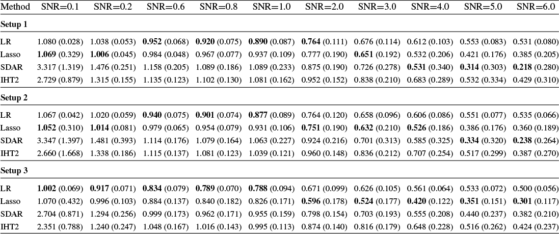


The performances of the estimators are compared in terms of the frequency at which they attained a given score. In Tables 4–6, the results for Setups 1–3 are provided. In each table, the frequency of a perfect score, as well as the score attained at the third, second, and first quantiles are exposed.
Experiment results for the two selection metrics (first setup)
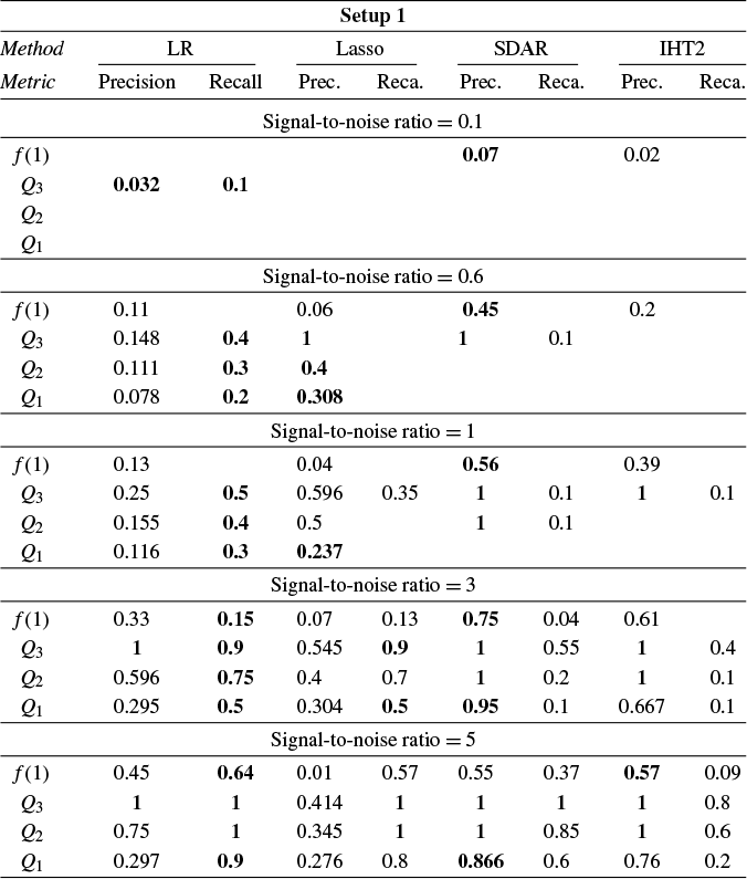
Note: Rows
 $f(1)$
and
$f(1)$
and
 $Q_i$
(
$Q_i$
(
 $i=1,2,3$
) show the frequency of reaching
$i=1,2,3$
) show the frequency of reaching
 $1$
and the third, second, and first quantiles. Blank cells =
$1$
and the third, second, and first quantiles. Blank cells =
 $0$
, and bold cells are the best values.
$0$
, and bold cells are the best values.
Experiment results for the two selection metrics (second setup)

Note: Rows
 $f(1)$
and
$f(1)$
and
 $Q_i$
(
$Q_i$
(
 $i=1,2,3$
) show the frequency of reaching
$i=1,2,3$
) show the frequency of reaching
 $1$
and the third, second, and first quantiles. Blank cells =
$1$
and the third, second, and first quantiles. Blank cells =
 $0$
, and bold cells are the best values.
$0$
, and bold cells are the best values.
Experiment results for the two selection metrics (third setup)

Note: Rows
 $f(1)$
and
$f(1)$
and
 $Q_i$
(
$Q_i$
(
 $i=1,2,3$
) show the frequency of reaching
$i=1,2,3$
) show the frequency of reaching
 $1$
and the third, second, and first quantiles. Blank cells =
$1$
and the third, second, and first quantiles. Blank cells =
 $0$
, and bold cells are the best values.
$0$
, and bold cells are the best values.
4.3 Implementations of the algorithms
For reproducibility, the code that generated the results of the experiment is provided on the website of the corresponding author. In the following paragraphs, the particular implementation of each algorithm is described.
-
• Loaded-Rifle. As suggested theoretically in Example 1, Algorithm 1 is initialized with the solution of a ten-fold cross-validated Lasso if the solution of the former is the nonzero vector. When the cross-validated Lasso is the zero vector, Algorithm 1 is initialized with a solution of Lasso tuned for having
$\overline {k}$
nonzero components (in the experiment, we fixed
$\overline {k}=36$
). The sparsity level of the output of Algorithm 1 is then selected through an additional ten-fold cross-validation. For each instance of LR, we set the step size
$\eta = 0.5 / \|\hat {\Sigma }_X\|_{\text {spec}}$
. -
• Two-Stage IHT. The two-stage IHT depends on a parameter fixing the dimension of a larger support on which the solution is pre-optimized. For comparability, we also fixed this parameter to
$k<\overline {k}=38$
, where k is selected by cross-validation. -
• SDAR. Following the theoretical and practical recommendations in Huang et al. (Reference Huang, Jiao, Liu and Lu2018), SDAR is initialized with the solution of a ridge regression with a tuning parameter
$2s \log (p) / n$
. Moreover, following the same recommendations, we preprocessed SDAR by dividing X and Y by
$\sqrt {n}$
(it appears in our experiments that SDAR is particularly sensitive to this transformation).


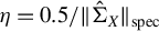


4.4 Results
Our evaluation of the LR method in estimating, prediction, and selection metrics in various experimental scenarios positions it as an effective, competitive, and often superior option for
 $l_0$
estimation, particularly in settings requiring both reliable variable selection and accurate estimation, even under limited SNR conditions.
$l_0$
estimation, particularly in settings requiring both reliable variable selection and accurate estimation, even under limited SNR conditions.
In terms of estimation accuracy, LR generally exhibits a favorable trend, with relative errors decreasing as SNR increases. In particular, for SNR values greater than 2, LR consistently achieves the lowest estimation errors, underscoring its effectiveness compared to other methods. Furthermore, the robustness of the LR estimates is reflected in its lower standardized errors compared to other estimators
 $l_0$
. These results highlight the suitability of LR variants for accurate parameter estimation tasks when moderate to high SNRs are attainable.
$l_0$
. These results highlight the suitability of LR variants for accurate parameter estimation tasks when moderate to high SNRs are attainable.
Prediction Accuracy: Prediction accuracy, measured by relative risk, reveals another strength of the LR. As soon as the SNR becomes sufficiently high for Lasso to outperform the null model (i.e., achieving a relative risk lower than that of the zero vector), but remains below one, LR surpasses all competing methods. This advantage is even more pronounced when covariates are highly correlated: in the third experimental setup, LR outperforms all competitors across all SNRs below one. These results make LR particularly appealing for predictive tasks in low-SNR and high-correlation environments, such as financial modeling (Hastie et al., Reference Hastie, Tibshirani and Tibshirani2020).
Selection Accuracy: The selection metrics clearly show that LR frequently outperforms its competitors in terms of recall. While other methods tend to prioritize precision, reducing false positives at the cost of increasing false negatives, LR adopts a more balanced strategy. Starting from a Lasso solution, it simultaneously reduces false positives and increases true positives. This behavior enables LR to recover part or all of the true support, even in low SNR regimes. Its superior performance in variable selection probably contributes to its advantages in both estimation and prediction. These findings support the adoption of LR in sparse recovery applications, where the accurate identification of relevant variables is critical.
In summary, LR demonstrates significant improvements in the accuracy of estimation, prediction, and selection over standard estimators
 $l_0$
and cross-validated Lasso. Its robustness in multiple metrics and SNR conditions suggests that LR variants offer substantial benefits for applications requiring strong statistical performance, particularly in domains characterized by low SNRs.
$l_0$
and cross-validated Lasso. Its robustness in multiple metrics and SNR conditions suggests that LR variants offer substantial benefits for applications requiring strong statistical performance, particularly in domains characterized by low SNRs.
5 CONCLUSION
This article proposes interpreting the parameter vector of the HDSLM as the product of a direction of interest, identified as the generalized eigenspace of a pair of measurable matrices, and a magnitude relative to this direction. This perspective offers new insights into linear regression and introduces a parameterization naturally aligned with several core ideas in economic theory.
For example, in a Cobb–Douglas production function, the logarithmic output Y can be written as
 $Y = X^\top \phi \nu $
, where
$Y = X^\top \phi \nu $
, where
 $\phi $
specifies factor shares summing to one and
$\phi $
specifies factor shares summing to one and
 $\nu $
reflects returns to scale. In the Cambridge equation (Fisher and Brown, Reference Fisher and Brown1911; Pigou, Reference Pigou1917), Y may represent money demand, X a vector of goods,
$\nu $
reflects returns to scale. In the Cambridge equation (Fisher and Brown, Reference Fisher and Brown1911; Pigou, Reference Pigou1917), Y may represent money demand, X a vector of goods,
 $\phi $
a price vector, and
$\phi $
a price vector, and
 $\nu $
the inverse of the velocity of money. In a currency context, Y could be a dollar amount, X quantities of goods, and
$\nu $
the inverse of the velocity of money. In a currency context, Y could be a dollar amount, X quantities of goods, and
 $\phi $
prices in euros, with
$\phi $
prices in euros, with
 $\nu $
representing the exchange rate. These examples illustrate that the choice of
$\nu $
representing the exchange rate. These examples illustrate that the choice of
 $\phi $
is context-specific and that normalizations, such as
$\phi $
is context-specific and that normalizations, such as
 $\|\phi \| = 1,$
are possible but not unique.
$\|\phi \| = 1,$
are possible but not unique.
Beyond its interpretive value, our approach connects linear regression to the GEP, expanding the class of estimators for linear models to include those suited to HD sparse settings. We exploit this connection by addressing the best subset selection problem through what we call the directional best subset selection, for which we establish a theoretical link to the classical formulation and derive the minimax convergence rate in the
 $l_2$
norm. Building on this, we adapt the RIFLE algorithm Tan et al., Reference Tan, Wang, Liu and Zhang2018 to construct an efficient estimator, LR, which achieves the minimax rate under sub-Gaussian assumptions and admits a CLT. To obtain this result, Proposition A3 in the Appendix provides sufficient conditions for the convergence in probability of a stochastic Cauchy product; this result may be of independent interest. These results are derived under the assumption of an exact sparsity structure for the parameter of interest
$l_2$
norm. Building on this, we adapt the RIFLE algorithm Tan et al., Reference Tan, Wang, Liu and Zhang2018 to construct an efficient estimator, LR, which achieves the minimax rate under sub-Gaussian assumptions and admits a CLT. To obtain this result, Proposition A3 in the Appendix provides sufficient conditions for the convergence in probability of a stochastic Cauchy product; this result may be of independent interest. These results are derived under the assumption of an exact sparsity structure for the parameter of interest
 $\beta $
. While common in the theoretical literature, this assumption can be overly restrictive in practical applications. A natural direction for future research is to extend our results to more general forms of approximate sparsity. Another important avenue is to address the unobservable bias identified in the CLT, either by characterizing its exact rate of convergence or by constructing a debiased version of the estimator.
$\beta $
. While common in the theoretical literature, this assumption can be overly restrictive in practical applications. A natural direction for future research is to extend our results to more general forms of approximate sparsity. Another important avenue is to address the unobservable bias identified in the CLT, either by characterizing its exact rate of convergence or by constructing a debiased version of the estimator.
Simulation results show that LR performs competitively, often outperforming existing
 $l_0$
-constrained estimators in estimation, variable selection, and prediction, while remaining computationally efficient even for large-scale problems. This combination of theoretical optimality and practical speed is rare in the current literature.
$l_0$
-constrained estimators in estimation, variable selection, and prediction, while remaining computationally efficient even for large-scale problems. This combination of theoretical optimality and practical speed is rare in the current literature.
While our focus has been on
 $l_0$
constraints and the RIFLE-based estimator, the identification result in Theorem 1 has broader implications. It suggests that other GEP estimators (e.g., Safo et al., Reference Safo, Ahn, Jeon and Jung2018; Jung, Ahn, and Jeon, Reference Jung, Ahn and Jeon2019; Yuan, Shen, and Zheng, Reference Yuan, Shen and Zheng2019) could be adapted to least squares problems constrained by other norms. More generally, the connection between least squares and GEP opens avenues for incorporating advanced numerical methods into HD estimation.
$l_0$
constraints and the RIFLE-based estimator, the identification result in Theorem 1 has broader implications. It suggests that other GEP estimators (e.g., Safo et al., Reference Safo, Ahn, Jeon and Jung2018; Jung, Ahn, and Jeon, Reference Jung, Ahn and Jeon2019; Yuan, Shen, and Zheng, Reference Yuan, Shen and Zheng2019) could be adapted to least squares problems constrained by other norms. More generally, the connection between least squares and GEP opens avenues for incorporating advanced numerical methods into HD estimation.
The scope of the theory presented in this article relies on several strong assumptions. Most notably, we work under an i.i.d. linear model. These assumptions are central to the spectral structure exploited by the GEP and to the identification arguments underlying our main results. Relaxing them—for instance, to allow for dependence, heteroskedasticity, or nonlinear structural relationships—would raise nontrivial theoretical challenges and falls outside the scope of the present analysis. Finally, although we have assumed exogeneity of the model throughout, extending Theorem 1 to instrumental variable (IV) settings remains a promising direction. Recent work (e.g., Belloni et al., Reference Belloni, Chen, Chernozhukov and Hansen2012; Fan and Liao, Reference Fan and Liao2014; Florens and Van Bellegem, Reference Florens and Van Bellegem2015; Chernozhukov, Hansen, and Spindler, Reference Chernozhukov, Hansen and Spindler2015; Gold, Lederer, and Tao, Reference Gold, Lederer and Tao2020) highlights the challenges of endogeneity in high dimensions. Extending our framework to IV models or systems of simultaneous equations, possibly allowing for vector-valued dependent variables and higher-rank GEPs, could substantially broaden its scope and impact.
COMPETING INTEREST STATEMENT
The authors declare no competing interests exist.
FUNDING STATEMENT
The authors received no specific funding for the work described in this article.
SUPPLEMENTARY MATERIAL
Sauvenier, M., & Van Bellegem, S. (2025). Supplementary Material on “Direction Identification and Minimax Estimation in High-Dimensional Sparse Regression via a Generalized Eigenvalue Approach.” To view, please visit: https://doi.org/10.1017/S0266466626100334.
A APPENDIX
This Appendix presents the proofs of all the results, except for the proof of Theorem 1, which is provided in Section 2. It also includes a detailed description of the RIFLE algorithm. The material is organized in the same order as in the main text. Technical lemmas and several standard auxiliary results used in the proofs are stated here, while their complete proofs are deferred to the Supplementary Material.
We note that the proof of Theorem 2, while correcting and extending the results in Tan et al. (Reference Tan, Wang, Liu and Zhang2018), employs the same techniques as in that paper and is therefore provided in the Supplementary Material. The proof of Proposition A2 relies on standard arguments as well, and is likewise presented in the Supplementary Material.
A.1 Proof of Theorem 1
Let
 $\mathcal {S}$
be the solution set of Problem (7) and observe that it is closed under scalar multiplication. Let
$\mathcal {S}$
be the solution set of Problem (7) and observe that it is closed under scalar multiplication. Let
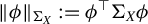 $\|\phi \|_{\Sigma _X}:=\phi ^\top \Sigma _X \phi $
, that is, the norm induced by
$\|\phi \|_{\Sigma _X}:=\phi ^\top \Sigma _X \phi $
, that is, the norm induced by
 $\Sigma _X$
and
$\Sigma _X$
and
 $\mathcal {S}_1:=\{\phi \in \mathcal {S}\text { s.t. } \phi=1\}$
and
$\mathcal {S}_1:=\{\phi \in \mathcal {S}\text { s.t. } \phi=1\}$
and
 $\mathcal {S}_2:=\{\phi \in \mathcal {S}\text { s.t. }\|\phi \|_{\Sigma _{X}}\not =1\}$
, hence we have
$\mathcal {S}_2:=\{\phi \in \mathcal {S}\text { s.t. }\|\phi \|_{\Sigma _{X}}\not =1\}$
, hence we have
 $$ \begin{align*} &\mathcal{S}=\mathcal{S}_1\sqcup \mathcal{S}_2 \text{ (disjoint union),}\\ &\text{if } \phi\in \mathcal{S}_2,\text{ then }\frac{\phi}{\|\phi\|_{\Sigma_{X}}}\in \mathcal{S}_1, \text{ and }\\ &\text{if }\phi\in \mathcal{S}_1, \text{ then }\alpha\phi\in \mathcal{S}_2\text{ for all }\alpha\not = 1. \end{align*} $$
Consider now the following problem whose solution set is equal to
 $\mathcal {S}_1$
:
$\mathcal {S}_1$
:
 $$ \begin{align} \operatorname{\mathrm{\arg\!\max}}_{\phi\in \mathbb{R}^p} \phi^\top \Sigma_{XY}\Sigma_{YX}\phi \hspace{5mm} \text{ such that } \|\phi\|_{\Sigma_{X}}^2=1. \end{align} $$
By the definition of
 $\|.\|_{\Sigma _{X}}$
, the Lagrangian of problem (A.1) is
$\|.\|_{\Sigma _{X}}$
, the Lagrangian of problem (A.1) is
 $$ \begin{align*} \mathcal{L}= \phi^\top \Sigma_{XY}\Sigma_{YX}\phi-\lambda(\phi^\top \Sigma_{X} \phi-1){.} \end{align*} $$
Computing
 $\nabla _\phi \mathcal {L}=0$
leads to
$\nabla _\phi \mathcal {L}=0$
leads to
 $$ \begin{align} \Sigma_{XY}\Sigma_{YX}\phi=\Sigma_{X}\phi\lambda, \end{align} $$
which is a scalar equation of the GEP of the matrix pair
 $\big (\Sigma _{XY}\Sigma _{YX}, \Sigma _{X}\big )$
. Pre-multiplying each side of this equation by
$\big (\Sigma _{XY}\Sigma _{YX}, \Sigma _{X}\big )$
. Pre-multiplying each side of this equation by
 $\phi ^\top $
identifies
$\phi ^\top $
identifies
 $\lambda $
as the maximum generalized eigenvalue, which is why we symbolize it by
$\lambda $
as the maximum generalized eigenvalue, which is why we symbolize it by
 $\lambda _{\max }$
. Observe that if
$\lambda _{\max }$
. Observe that if
 $\phi $
satisfies (A.2), then
$\phi $
satisfies (A.2), then
 $\alpha \phi $
also satisfies this equation for any
$\alpha \phi $
also satisfies this equation for any
 $\alpha \in \mathbb {R}$
. This last remark allows us to conclude that
$\alpha \in \mathbb {R}$
. This last remark allows us to conclude that
 $$ \begin{align*} \mathrm{Ker} \big(\Sigma_{XY}\Sigma_{YX}-\lambda_{\max}\Sigma_{X}\big)=\mathcal{S}_1\sqcup\mathcal{S}_2=\mathcal{S}, \end{align*} $$
which is the result to be proven.
A.2 Statement and Proof of Proposition A1
The following proposition confirms that the solution set
 $\hat {\Phi }$
identifies the direction of the best subset selection solution.
$\hat {\Phi }$
identifies the direction of the best subset selection solution.
Proposition A1. Let
 $Y \in \mathbb {R}^n$
and
$Y \in \mathbb {R}^n$
and
 $X \in \mathbb {R}^{n \times p}$
. For a fixed integer
$X \in \mathbb {R}^{n \times p}$
. For a fixed integer
 $k \in \mathbb {N}$
, let
$k \in \mathbb {N}$
, let
 $\hat {\beta }$
denote a solution of the best subset selection problem defined in (3), and let
$\hat {\beta }$
denote a solution of the best subset selection problem defined in (3), and let
 $\hat {\phi }$
denote a solution of the directional best subset selection defined in (4). Then, conditionally on the uniqueness of
$\hat {\phi }$
denote a solution of the directional best subset selection defined in (4). Then, conditionally on the uniqueness of
 $\hat {\beta }$
and on
$\hat {\beta }$
and on
 $\min _{v \in \mathbb {R}^p, \|v\|_0 \leq k} v^\top \hat {\Sigma }_X v> 0$
, it holds
$\min _{v \in \mathbb {R}^p, \|v\|_0 \leq k} v^\top \hat {\Sigma }_X v> 0$
, it holds
 $\hat {\beta }/\|\hat {\beta }\|_2 = \hat {\phi }/\|\hat {\phi }\|_2$
almost surely. Furthermore, if
$\hat {\beta }/\|\hat {\beta }\|_2 = \hat {\phi }/\|\hat {\phi }\|_2$
almost surely. Furthermore, if
 $\hat {\upsilon } = \operatorname {\mathrm {\arg \!\min }}_{m \in \mathbb {R}} n^{-1} \|Y - X \hat {\phi } m\|_2^2$
, then
$\hat {\upsilon } = \operatorname {\mathrm {\arg \!\min }}_{m \in \mathbb {R}} n^{-1} \|Y - X \hat {\phi } m\|_2^2$
, then
 $\hat {\phi }\hat {\upsilon } = \hat {\beta }$
almost surely.
$\hat {\phi }\hat {\upsilon } = \hat {\beta }$
almost surely.
Proof. Let
 $\mathcal {O}(p,k):=\{v\in \mathbb {R}^p; \|v\|_0=k\}$
. Observe that for any
$\mathcal {O}(p,k):=\{v\in \mathbb {R}^p; \|v\|_0=k\}$
. Observe that for any
 $v\in \mathcal {O}(p,k),$
there exists an infinity of
$v\in \mathcal {O}(p,k),$
there exists an infinity of
 $(\phi ,m)\in \mathcal {O}(p,k) \times \mathbb {R}$
such that
$(\phi ,m)\in \mathcal {O}(p,k) \times \mathbb {R}$
such that
 $\phi m=v$
. Hence, note that if
$\phi m=v$
. Hence, note that if
 $(\hat {\phi },\hat {m}) \in \operatorname {\mathrm {\arg \!\min }} _{(\phi ,m)\in \mathcal {O}(p,k) \times \mathbb {R}} n^{-1} \|Y-X \phi m\|_2^2$
, then
$(\hat {\phi },\hat {m}) \in \operatorname {\mathrm {\arg \!\min }} _{(\phi ,m)\in \mathcal {O}(p,k) \times \mathbb {R}} n^{-1} \|Y-X \phi m\|_2^2$
, then
 $\hat {\beta }= \hat {\phi } \hat {m}$
almost surely. Now, observe that for any
$\hat {\beta }= \hat {\phi } \hat {m}$
almost surely. Now, observe that for any
 $\phi \in \mathcal {O}(p,k)$
, we have
$\phi \in \mathcal {O}(p,k)$
, we have
 $$ \begin{align*} \operatorname{\mathrm{\arg\!\min}}_{m\in \mathbb{R}}\frac{1}{n} \|Y-X\phi m\|_2^2 = \frac{\phi^\top X^\top Y}{\phi^\top X^\top X \phi}. \end{align*} $$
Then, in particular, if
 $\hat {\phi }\in \operatorname {\mathrm {\arg \!\min }}_{\phi \in \mathcal {O}(p,k)}n^{-1}\|Y-(X\phi \phi ^\top X Y)/\phi ^\top X^\top X\phi )\|_2^2$
, we have
$\hat {\phi }\in \operatorname {\mathrm {\arg \!\min }}_{\phi \in \mathcal {O}(p,k)}n^{-1}\|Y-(X\phi \phi ^\top X Y)/\phi ^\top X^\top X\phi )\|_2^2$
, we have
 $\hat {\beta }/\|\hat {\beta }\|_2 = \hat {\phi }/\|\hat {\phi }\|_2$
a.s. Finally, computations similar to the ones in the proof of Theorem 1 lead to
$\hat {\beta }/\|\hat {\beta }\|_2 = \hat {\phi }/\|\hat {\phi }\|_2$
a.s. Finally, computations similar to the ones in the proof of Theorem 1 lead to
 $$ \begin{align*} \operatorname{\mathrm{\arg\!\min}}_{\hat{\phi} \in \mathcal{O}(p,k)}\frac{1}{n}\|Y-\frac{X\hat{\phi} \hat{\phi}^\top X Y}{\hat{\phi}^\top X^\top X\hat{\phi}}\|_2^2 = \operatorname{\mathrm{\arg\!\max}} _{\hat{\phi} \in \mathcal{O}(p,k)} \frac{\hat{\phi}^\top X^\top Y Y^\top X \hat{\phi}}{\hat{\phi}^\top X^\top X \hat{\phi}n}, \end{align*} $$
that gives the result.
A.3 Algorithm: Truncated Rayleigh flow method (RIFLE)
Algorithm 2. Truncated Rayleigh flow method (RIFLE).
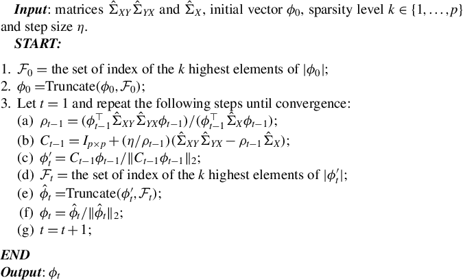
Tan et al. (Reference Tan, Wang, Liu and Zhang2018) provide the computational complexity of the algorithm, that is, the sum between two terms: First,
 $O(p)$
for selecting the k largest elements of a p-dimensional vector and second,
$O(p)$
for selecting the k largest elements of a p-dimensional vector and second,
 $O(kp)$
to take the product between a truncated vector and a matrix with columns restricted to the set
$O(kp)$
to take the product between a truncated vector and a matrix with columns restricted to the set
 $F_t$
and to calculate the difference between two matrices with columns restricted to the set
$F_t$
and to calculate the difference between two matrices with columns restricted to the set
 $F_t$
(Tan et al., Reference Tan, Wang, Liu and Zhang2018).
$F_t$
(Tan et al., Reference Tan, Wang, Liu and Zhang2018).
A.4 Proof of Proposition 1
In order to prove Proposition 1, we need the following proposition.
A.4.1 Proposition A2
Proposition A2. In model (1), assume that
 $Y_1$
,
$Y_1$
,
 $X_{1,1}, \dots , X_{1,p(n)}$
are sub-Gaussian, that
$X_{1,1}, \dots , X_{1,p(n)}$
are sub-Gaussian, that
 $\Sigma _X := \mathbb {E}(X_1 X_1^\top )$
is positive definite, and that
$\Sigma _X := \mathbb {E}(X_1 X_1^\top )$
is positive definite, and that
 $\|\beta \|_0 = s$
. Let
$\|\beta \|_0 = s$
. Let
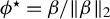 $\phi ^\star =\beta /\|\beta \|_{2}$
,
$\phi ^\star =\beta /\|\beta \|_{2}$
,
 $\hat {\Sigma }_X=X^\top X/n,$
and
$\hat {\Sigma }_X=X^\top X/n,$
and
 $k'=Cs$
for
$k'=Cs$
for
 $C>1$
. If
$C>1$
. If
 $s\log (p/s)/n=o(1)$
and
$s\log (p/s)/n=o(1)$
and
 $s/p=o(1)$
, then
$s/p=o(1)$
, then
 $$ \begin{align*} \varepsilon(k')=O_p(\sqrt{\frac{s\log(p/s)}{n}}) \end{align*} $$
and
 $$ \begin{align*} \rho( \hat{\Sigma}_X-\Sigma_X, k')=O_p(\sqrt{\frac{s\log(p/s)}{n}}). \end{align*} $$
Proof. The result follows directly from Lemmas 4 and 5 stated and proved in the Supplementary Material.
A.4.2 Proof of Proposition 1
First, we note that since
 $\langle \phi ^\star , \hat {\phi }(t) \rangle _2 \geq 0$
, then
$\langle \phi ^\star , \hat {\phi }(t) \rangle _2 \geq 0$
, then
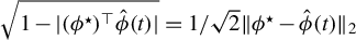 $\sqrt {1 - |(\phi ^\star )^\top \hat {\phi }(t)|}=1/\sqrt {2}\|\phi ^\star - \hat {\phi }(t)\|_2$
. Second, we observe that since we can choose
$\sqrt {1 - |(\phi ^\star )^\top \hat {\phi }(t)|}=1/\sqrt {2}\|\phi ^\star - \hat {\phi }(t)\|_2$
. Second, we observe that since we can choose
 $t=t(n)$
, we can choose it sufficiently fast to ensure that for any positive constant
$t=t(n)$
, we can choose it sufficiently fast to ensure that for any positive constant
 $M_1$
, there is a positive constant M and
$M_1$
, there is a positive constant M and
 $N_1\in \mathbb {N}$
such that for all
$N_1\in \mathbb {N}$
such that for all
 $n>N_1,$
 $$ \begin{align*} \mathbb{P}\Big( \|\phi^\star - \hat{\phi}(t)\|_2> \nu^{t} \sqrt{\xi} + \sqrt{\frac{s\log(p/s)}{n}} M_1\Big)\leq \mathbb{P}\Big( \|\phi^\star - \hat{\phi}(t)\|_2 > \sqrt{\frac{s\log(p/s)}{n}} M\Big), \end{align*} $$
where
 $ \nu ^{t} \sqrt {\xi }$
is as in Theorem 2.
$ \nu ^{t} \sqrt {\xi }$
is as in Theorem 2.
Hence, concentrating on
 $\mathbb {P}\Big ( \|\phi ^\star - \hat {\phi }(t)\|_2> \sqrt {\frac {s\log (p/s)}{n}} M\Big )$
, by the Law of Total Probability, for all positive constants
$\mathbb {P}\Big ( \|\phi ^\star - \hat {\phi }(t)\|_2> \sqrt {\frac {s\log (p/s)}{n}} M\Big )$
, by the Law of Total Probability, for all positive constants
 $c,$
$c,$
 $$ \begin{align*} &\mathbb{P}\Big( \|\phi^\star - \hat{\phi}(t)\|_2> \sqrt{\frac{s\log(p/s)}{n}} M\Big) \\ &\leq \mathbb{P}\Big( \|\phi^\star - \hat{\phi}(t)\|_2 > \sqrt{\frac{s\log(p/s)}{n}} M \Big| \|\phi^\star-\phi_{0}\|_2 < c\Big) + \mathbb{P} \Big(\|\phi^\star-\phi_{0}\|_2 \geq c\Big). \end{align*} $$
If c is such that
 $|\langle \phi ^\star , \phi _{0} \rangle _2 | \geq 1- \nu ^2 \xi $
as in Theorem 2, then we can choose
$|\langle \phi ^\star , \phi _{0} \rangle _2 | \geq 1- \nu ^2 \xi $
as in Theorem 2, then we can choose
 $t=t(n)$
such that by Proposition A2 and Theorem 2 for every
$t=t(n)$
such that by Proposition A2 and Theorem 2 for every
 $\epsilon _2>0,$
there exists an
$\epsilon _2>0,$
there exists an
 $N_2$
such that for every
$N_2$
such that for every
 $n>N_2,$
 $$ \begin{align*} \mathbb{P}\Big( \|\phi^\star - \hat{\phi}(t)\|_2> \sqrt{\frac{s\log(p/s)}{n}} M \Big| \|\phi^\star-\phi_{0}\|_2 < c\Big) \leq \epsilon_1. \end{align*} $$
Moreover, since
 $\alpha _n=o(1)$
, for every
$\alpha _n=o(1)$
, for every
 $\epsilon _3>0$
, there exists
$\epsilon _3>0$
, there exists
 $N_3$
such that for every
$N_3$
such that for every
 $n\geq N_3,$
 $$ \begin{align*} \mathbb{P} \Big(\|\phi^\star-\phi_{0}\|_2 \geq c\Big) < \epsilon_3. \end{align*} $$
Hence, for every
 $\epsilon>0$
, choose
$\epsilon>0$
, choose
 $\epsilon _2=\epsilon _3=\epsilon /2$
, and let
$\epsilon _2=\epsilon _3=\epsilon /2$
, and let
 $N=N_1+N_2+N_3$
, and observe that, as intended, for every
$N=N_1+N_2+N_3$
, and observe that, as intended, for every
 $n\geq N,$
 $$ \begin{align*} \mathbb{P}\Big( \|\phi^\star - \hat{\phi}(t)\|_2> \sqrt{\frac{s\log(p/s)}{n}} M\Big) < \epsilon. \end{align*} $$
A.5 Proof of Proposition 2
Let
 $\upsilon =\|\beta \|_{2}$
and
$\upsilon =\|\beta \|_{2}$
and
 $U:=Y-X\beta $
, straightforward computations give
$U:=Y-X\beta $
, straightforward computations give
 $$ \begin{align*} \hat{\upsilon}&=\frac{\hat{\phi}^\top X^\top Y}{\hat{\phi}^\top X^\top X \hat{\phi}} = \upsilon+ \frac{\upsilon}{\hat{\phi}^\top \hat{\Sigma}_X \hat{\phi}} \big(\hat{\phi}^\top \hat{\Sigma}_X (\phi^\star - \hat{\phi}) + \frac{\hat{\phi}^\top X^\top U }{n\upsilon}\big), \end{align*} $$
where the second equality is obtained by adding zero and simplifying. Hence, we have an equality for
 $\hat {\upsilon }-\upsilon $
that we now use to obtain an inequality. Let
$\hat {\upsilon }-\upsilon $
that we now use to obtain an inequality. Let
 $P\in \mathcal {P}(\mathcal {F}(p,2s))$
be defined as in Section 3.1, and
$P\in \mathcal {P}(\mathcal {F}(p,2s))$
be defined as in Section 3.1, and
 $PP^\top \hat {\phi }= \hat {\phi }$
and
$PP^\top \hat {\phi }= \hat {\phi }$
and
 $PP^\top (\phi ^\star - \hat {\phi })=(\phi ^\star - \hat {\phi })$
.
$PP^\top (\phi ^\star - \hat {\phi })=(\phi ^\star - \hat {\phi })$
.
Observe that
 $$ \begin{align*} \hat{\phi}^\top \hat{\Sigma}_X (\phi^\star - \hat{\phi}) &=\hat{\phi}^\top PP^\top \hat{\Sigma}_X PP^\top(\phi^\star - \hat{\phi})\leq \overline{\kappa} \|\phi^\star-\hat{\phi}\|_2, \end{align*} $$
where the second equation is obtained by the Cauchy–Schwarz inequality, the submultiplicativity of the spectral norm, and
 $\|P\|_{\mathrm {spec}}=1$
. Hence,
$\|P\|_{\mathrm {spec}}=1$
. Hence,
 $$ \begin{align*} |\hat{\upsilon}-\upsilon| &\leq \frac{v}{\underline{\kappa}} \bigg( \overline{\kappa} \|\phi^\star-\hat{\phi}\|_2 + \frac{1}{\upsilon} \|\frac{P^\top X^\top U}{n}\|_2 \bigg), \end{align*} $$
which implies
 $|\hat {\upsilon }-\upsilon |= O_p\big (\alpha _n) + O_p\big (\sqrt {2s/n}\big )=O_p\big (\alpha _n)$
. And since
$|\hat {\upsilon }-\upsilon |= O_p\big (\alpha _n) + O_p\big (\sqrt {2s/n}\big )=O_p\big (\alpha _n)$
. And since
 $$ \begin{align*} \|\hat{\beta}- \beta \|^2_2 &=\|\hat{\upsilon} \hat{\phi} -\upsilon \phi^\star \|^2_2 & \\ &= \hat{\upsilon}^2 - 2\hat{\upsilon} \upsilon \langle \hat{\phi}, \phi^\star \rangle_2 + \upsilon^2 & (\text{Since }\|\hat{\phi}\|_2=\|\phi^\star \|_2=1)\\ &= (\hat{\upsilon} - \upsilon )^2 + 2\hat{\upsilon} \upsilon (1-\langle \hat{\phi}, \phi^\star \rangle_2)\\ &= (\hat{\upsilon} - \upsilon )^2 + \hat{\upsilon} \upsilon \|\hat{\phi}-\phi^\star\|_2^2& (\text{Since }\langle \hat{\phi}, \phi^\star \rangle_2 \geq 0)\\ &= (\hat{\upsilon} - \upsilon )^2 + \big((\hat{\upsilon}-\upsilon)\upsilon + \upsilon^2 \big) \|\hat{\phi}-\phi^\star\|_2^2{.}& \end{align*} $$
Since
 $|\hat {\upsilon } - \upsilon |=O_p(\alpha _n)$
,
$|\hat {\upsilon } - \upsilon |=O_p(\alpha _n)$
,
 $(\hat {\upsilon } - \upsilon )^2=O_p(\alpha ^2)$
and
$(\hat {\upsilon } - \upsilon )^2=O_p(\alpha ^2)$
and
 $(\hat {\upsilon }-\upsilon )\upsilon + \upsilon ^2=O_p(1)$
, the result follows.
$(\hat {\upsilon }-\upsilon )\upsilon + \upsilon ^2=O_p(1)$
, the result follows.
A.6 Statement and proof of A3
Proposition A3. Let
 $\{a_i\}_{i=0}^m$
and
$\{a_i\}_{i=0}^m$
and
 $\{b_i\}_{i=0}^m$
be two sequences of positive random variables such that
$\{b_i\}_{i=0}^m$
be two sequences of positive random variables such that
 $m=m(n),$
where
$m=m(n),$
where
 $m \rightarrow \infty $
as
$m \rightarrow \infty $
as
 $n \rightarrow \infty $
. If
$n \rightarrow \infty $
. If
 $\{a_i\}_{i=0}^m=o_p(1)$
,
$\{a_i\}_{i=0}^m=o_p(1)$
,
 $\sup _{i\in \{0,\ldots ,m\}}|a_i|=O_p(1)$
and it exists a finite
$\sup _{i\in \{0,\ldots ,m\}}|a_i|=O_p(1)$
and it exists a finite
 $M\in \mathbb {R}$
such that
$M\in \mathbb {R}$
such that
 $\lim _{n \rightarrow \infty }\sum _{i=0}^{m(n)}b_i=M$
almost surely. Then,
$\lim _{n \rightarrow \infty }\sum _{i=0}^{m(n)}b_i=M$
almost surely. Then,
 $\sum _{i=0}^{m} a_{m-i}b_i =o_p(1)$
.
$\sum _{i=0}^{m} a_{m-i}b_i =o_p(1)$
.
Proof. Since
 $\sup _{i\in \{0,\ldots ,m\}} a_i=O_p(1)$
, for all
$\sup _{i\in \{0,\ldots ,m\}} a_i=O_p(1)$
, for all
 $\epsilon>0$
, there exist
$\epsilon>0$
, there exist
 $N_1\in \mathbb {N}$
and
$N_1\in \mathbb {N}$
and
 $C>0$
such that for all
$C>0$
such that for all
 $m>m(N_1)$
and all
$m>m(N_1)$
and all
 $\gamma>0,$
we have
$\gamma>0,$
we have
 $$ \begin{align*} \mathbb{P} \bigg(\sum_{i=0}^{m} a_{m-i}b_i> \gamma \bigg) &\leq \mathbb{P} \bigg(\sum_{i=0}^{m}a_{m-i}b_i > \gamma \bigg| \sup_{i\in \{0,\ldots,m\}}a_i \leq C\bigg) + \mathbb{P} \bigg( \sup_{i\in \{0,\ldots,m\}}a_i > C\bigg) \\ &=\mathbb{P} \bigg(\sum_{i=0}^{m}a_{m-i}b_i > \gamma \bigg| \sup_{i\in \{0,\ldots,m\}}a_i \leq C\bigg) + \epsilon/2. \end{align*} $$
Now, since
 $\lim _{n\rightarrow \infty }\sum _{i=0}^{m}b_i=M$
a.s., for all
$\lim _{n\rightarrow \infty }\sum _{i=0}^{m}b_i=M$
a.s., for all
 $\alpha>0$
, there exists
$\alpha>0$
, there exists
 $N_2\in \mathbb {N}$
such that for all
$N_2\in \mathbb {N}$
such that for all
 $m\geq m(N_2),$
we have
$m\geq m(N_2),$
we have
 $\sum _{m\geq m(N_2)}b_i \leq \alpha /(2C) \text { almost surely.}$
Consequently, we have for any
$\sum _{m\geq m(N_2)}b_i \leq \alpha /(2C) \text { almost surely.}$
Consequently, we have for any
 $\gamma>0$
and all
$\gamma>0$
and all
 $m>M(N_2)$
that
$m>M(N_2)$
that
 $$ \begin{align*} \mathbb{P} \bigg(\sum_{i=0}^{m}a_{m-i}b_i> \gamma \bigg| \sup_{i\in \{0,\ldots,m\}}a_i \leq C\bigg) \leq \mathbb{P} \bigg(\sum_{i=0}^{m(N_2)}a_{m-i}b_i + \frac{\alpha}{2} > \gamma \bigg| \sup_{i\in \{0,\ldots,m\}}a_i \leq C\bigg). \end{align*} $$
Note now that since
 $\{a_i\}_{i=0}^m=o_p(1)$
, for any
$\{a_i\}_{i=0}^m=o_p(1)$
, for any
 $\alpha ,\tilde {\epsilon }>0,$
there exists
$\alpha ,\tilde {\epsilon }>0,$
there exists
 $N_3\in \mathbb {N}$
such that for all
$N_3\in \mathbb {N}$
such that for all
 $m>m(N_3),$
we have
$m>m(N_3),$
we have
 $$ \begin{align*} \mathbb{P}\bigg(a_m> \frac{\alpha}{2m(N_2)M}\bigg) < \frac{\tilde{\epsilon}}{(m(N_2)+1)}, \end{align*} $$
which implies by a union bound that for all
 $m> m(N_2)+m(N_3),$
 $$ \begin{align*} \mathbb{P} \bigg( \sup_{i\in \{0,\ldots,m(N_2)\}} a_{m-i}> \frac{\alpha}{2m(N_2)M}\bigg) \leq \tilde{\epsilon}. \end{align*} $$
Hence, for all
 $m> m(N_2)+m(N_3),$
 $$ \begin{align*} & \mathbb{P} \bigg(\sum_{i=0}^{m(N_2)}a_{m-i}b_i + \frac{\alpha}{2}> \gamma \bigg| \sup_{i\in \{0,\ldots,m\}}a_i \leq C\bigg) \\ & \leq\mathbb{P} \bigg(\sum_{i=0}^{m(N_2)}a_{m-i}b_i + \frac{\alpha}{2} > \gamma \bigg| \{\sup_{i\in \{0,\ldots,m\}}a_i \leq C\} \cap \{ \sup_{i\in \{0,\ldots,m(N_2)\}} a_{m(N_2)-i}< \frac{\alpha}{2m(N_2)M}\}\bigg)\\ & + \mathbb{P} \bigg( \sup_{i\in \{0,\ldots,m(N_2)\}} a_{m(N_2)-i}> \frac{\alpha}{2m(N_2)M}\ \bigg| \{\sup_{i\in \{0,\ldots,m\}}a_i \leq C\} \bigg). \end{align*} $$
And since for any events A and B such that
 $\mathbb {P}(B)>0$
, we have
$\mathbb {P}(B)>0$
, we have
 $$ \begin{align*} \mathbb{P}(A)&=\mathbb{P} (A|B)\mathbb{P} (B) + \mathbb{P} (A|\bar{B}) \mathbb{P} (\bar{B})\\ \mathbb{P}(A)&\geq \mathbb{P} (A|B) \mathbb{P} (B)\\ \frac{\mathbb{P}(A)}{1-\mathbb{P}(\bar{B})}&\geq \mathbb{P}(A|B) \end{align*} $$
and by choosing the events
 $A:=\{\sup _{i\in \{0,\ldots ,m(N_2)\}} a_{m(N_2)-i}<\alpha /(2m(N_2)M\}$
and
$A:=\{\sup _{i\in \{0,\ldots ,m(N_2)\}} a_{m(N_2)-i}<\alpha /(2m(N_2)M\}$
and
 $B=\{\sup _{i\in \{0,\ldots ,m\}}a_i \leq C\}$
, we have for any
$B=\{\sup _{i\in \{0,\ldots ,m\}}a_i \leq C\}$
, we have for any
 $\epsilon , \tilde {\epsilon }$
, that there exist
$\epsilon , \tilde {\epsilon }$
, that there exist
 $N_2$
and C such that
$N_2$
and C such that
 $$ \begin{align*} \mathbb{P} \bigg( \sup_{i\in \{0,\ldots,m(N_2)\}} a_{m(N_2)-i}> \frac{\alpha}{2m(N_2)M}\ \bigg| \{\sup_{i\in \{0,\ldots,m\}}a_i \leq C\} \bigg) \leq \frac{\tilde{\epsilon}}{1-\epsilon/2}. \end{align*} $$
Hence, for every
 $\epsilon ,$
we choose
$\epsilon ,$
we choose
 $\tilde {\epsilon }$
such that
$\tilde {\epsilon }$
such that
 $\tilde {\epsilon }/(1-\epsilon /2)< \epsilon /2$
. Observe that this choice only affects
$\tilde {\epsilon }/(1-\epsilon /2)< \epsilon /2$
. Observe that this choice only affects
 $N_3$
. As a consequence, we have for all
$N_3$
. As a consequence, we have for all
 $m> m(N_2)+m(N_3),$
 $$ \begin{align*} & \mathbb{P} \bigg(\sum_{i=0}^{m(N_2)}a_{m-i}b_i + \frac{\alpha}{2}> \gamma \bigg| \sup_{i\in \{0,\ldots,m\}}a_i \leq C\bigg) \\ & \leq\mathbb{P} \bigg(\sum_{i=0}^{m(N_2)}a_{m-i}b_i + \frac{\alpha}{2} > \gamma \bigg|\\ & \{\sup_{i\in \{0,\ldots,m\}}a_i \leq C\} \cap \{ \sup_{i\in \{0,\ldots,m(N_2)\}} a_{m(N_2)-i}< \frac{\alpha}{2m(N_2)M}\}\bigg) + \epsilon/2{,} \end{align*} $$
where
 $$ \begin{align*} & \mathbb{P} \bigg(\sum_{i=0}^{m(N_2)}a_{m-i}b_i + \frac{\alpha}{2}> \gamma \bigg| \{\sup_{i\in \{0,\ldots,m\}}a_i \leq C\} \cap \{ \sup_{i\in \{0,\ldots,m(N_2)\}} a_{m(N_2)-i}< \frac{\alpha}{2m(N_2)M}\}\bigg)\\ & \leq \mathbb{P} \bigg(\frac{\alpha}{2} + \frac{\alpha}{2}> \gamma \bigg| \{\sup_{i\in \{0,\ldots,m\}}a_i \leq C\} \cap \{ \sup_{i\in \{0,\ldots,m(N_2)\}} a_{m(N_2)-i}< \frac{\alpha}{2m(N_2)M}\}\bigg)\\ & \leq \mathbb{P} \bigg(\alpha> \gamma \bigg| \{\sup_{i\in \{0,\ldots,m\}}a_i \leq C\} \cap \{ \sup_{i\in \{0,\ldots,m(N_2)\}} a_{m(N_2)-i}< \frac{\alpha}{2m(N_2)M}\}\bigg){.} \end{align*} $$
And since we can pick
 $\alpha>0$
as small as we want, for any fixed
$\alpha>0$
as small as we want, for any fixed
 $\gamma>0,$
we can make the probability in the last inequality equal to zero. Hence, for all
$\gamma>0,$
we can make the probability in the last inequality equal to zero. Hence, for all
 $\gamma ,\epsilon>0$
, there exists
$\gamma ,\epsilon>0$
, there exists
 $N_1,N_2,N_3\in \mathbb {N}$
such that for all
$N_1,N_2,N_3\in \mathbb {N}$
such that for all
 $m>m(N_1)+ m(N_2)+m(N_3),$
we have
$m>m(N_1)+ m(N_2)+m(N_3),$
we have
 $\mathbb {P} (\sum _{i=0}^{m} a_{m-i}b_i> \gamma )<\epsilon ,$
which is what is needed to be proven.
$\mathbb {P} (\sum _{i=0}^{m} a_{m-i}b_i> \gamma )<\epsilon ,$
which is what is needed to be proven.
A.7 Statement, Comments, and Proof of Proposition A4
Proposition A4. For all
 $n\in \mathbb {N}$
, let
$n\in \mathbb {N}$
, let
 $Y\in \mathbb {R}^n$
and
$Y\in \mathbb {R}^n$
and
 $X\in \mathbb {R}^{n \times p}$
be random functions i.i.d. across rows. For all
$X\in \mathbb {R}^{n \times p}$
be random functions i.i.d. across rows. For all
 $n\in \mathbb {N,}$
assume that
$n\in \mathbb {N,}$
assume that
 $\Sigma _X:=\mathbb {E}(X_1X_1^\top )$
is positive definite and there exists
$\Sigma _X:=\mathbb {E}(X_1X_1^\top )$
is positive definite and there exists
 $\beta \in \mathbb {R}^p$
s.t.
$\beta \in \mathbb {R}^p$
s.t.
 $\mathbb {E}(Y_1|X_1)=X_1^\top \beta $
. Let
$\mathbb {E}(Y_1|X_1)=X_1^\top \beta $
. Let
 $\phi ^\star =\beta /\|\beta \|_{2}$
and
$\phi ^\star =\beta /\|\beta \|_{2}$
and
 $s=\|\beta \|_0$
. Let
$s=\|\beta \|_0$
. Let
 $t, \eta ,\phi _t, C_{t-1,}$
and
$t, \eta ,\phi _t, C_{t-1,}$
and
 $\phi _0$
be as in Algorithm 1. Finally, let
$\phi _0$
be as in Algorithm 1. Finally, let
 $\tilde {\phi _t}=C_{t-1}\phi _{t-1}$
. Then, for every
$\tilde {\phi _t}=C_{t-1}\phi _{t-1}$
. Then, for every
 $t\geq 2,$
 $$ \begin{align*} \phi_t=\ &\bigg( \prod_{m=1}^t \Gamma_{t-m}\bigg) \phi_0 + \sum_{m=0}^{t-1} \bigg( \prod_{l=1}^m\Gamma_{t-l}\bigg)(\phi_{t-l}-\tilde{\phi}_{t-l})\\ & + \eta \sum_{m=0}^{t-1} \bigg( \prod_{l=1}^m\Gamma_{t-l}\bigg) \frac{\phi_{t-1-m}^\top \hat{\Sigma}_X \phi_{t-1-m}}{\phi_{t-1-m}^\top \hat{\Sigma}_X \phi^\star + \phi_{t-1-m}^\top \frac{X^\top U}{\|\beta\|_{2}n}} \bigg( \hat{\Sigma}_X \phi^\star + \frac{X^\top U}{\| \beta\|_{2}n}\bigg) \end{align*} $$
almost surely, where
 $\Gamma _i=(I_{p\times p} - \eta \hat {\Sigma }_X)Q_{i}$
for any
$\Gamma _i=(I_{p\times p} - \eta \hat {\Sigma }_X)Q_{i}$
for any
 $i\in \mathbb {N}$
.
$i\in \mathbb {N}$
.
This proposition analyzes the output of Algorithm 2. The first term explains the numerical dependence of
 $\phi _t$
on
$\phi _t$
on
 $\phi _0$
. From Lemma A1, one can show that there exists
$\phi _0$
. From Lemma A1, one can show that there exists
 $\eta $
, making this dependence go to zero in probability as
$\eta $
, making this dependence go to zero in probability as
 $t\rightarrow \infty $
. The second term, which is a Cauchy product, explains the impact of the normalization in Step 3.c) and of the truncation in Step 3.e) of Algorithm 2. Using Proposition A3 to prove that this term is
$t\rightarrow \infty $
. The second term, which is a Cauchy product, explains the impact of the normalization in Step 3.c) and of the truncation in Step 3.e) of Algorithm 2. Using Proposition A3 to prove that this term is
 $o_p(1)$
is a key step in the proof of Theorem 3. The third term, which is also a Cauchy product, is shown to converge to
$o_p(1)$
is a key step in the proof of Theorem 3. The third term, which is also a Cauchy product, is shown to converge to
 $\phi ^\star $
by using Proposition A5.
$\phi ^\star $
by using Proposition A5.
Proof. Let
 $f(\phi _{t}):=\rho _t=(\phi _{t}^\top \hat {\Sigma }_{XY}\hat {\Sigma }_{YX}\phi _{t})/(\phi _{t}^\top \hat {\Sigma }_X\phi _{t})$
. As a consequence, we have
$f(\phi _{t}):=\rho _t=(\phi _{t}^\top \hat {\Sigma }_{XY}\hat {\Sigma }_{YX}\phi _{t})/(\phi _{t}^\top \hat {\Sigma }_X\phi _{t})$
. As a consequence, we have
 $\nabla _{\phi _{t}} f= (2/\phi _{t}^\top \hat {\Sigma }_X \phi _{t}) \big ( \hat {\Sigma }_{XY}\hat {\Sigma }_{YX}\phi _{t} - f(\phi _{t}) \hat {\Sigma }_X\phi _{t} \big )$
. Moreover, note that
$\nabla _{\phi _{t}} f= (2/\phi _{t}^\top \hat {\Sigma }_X \phi _{t}) \big ( \hat {\Sigma }_{XY}\hat {\Sigma }_{YX}\phi _{t} - f(\phi _{t}) \hat {\Sigma }_X\phi _{t} \big )$
. Moreover, note that
 $$ \begin{align*} \phi_{t}^\top \hat{\Sigma}_{XY}\hat{\Sigma}_{YX}\phi_{t} &= \left( \frac{\phi_{t}^\top X^\top Y}{n} \right)^2 \\ &= \left( \frac{\phi_{t}^\top X^\top X\beta}{n}+ \frac{\phi^\top X^\top U}{n} \right)^2 \\ &= \left( \frac{\phi_{t}^\top X^\top X \phi_{t}\|\beta\|_{2}}{n}+ \frac{\phi_{t}^\top X^\top X (\phi^\star-\phi_{t})\|\beta\|_{2}}{n}+\frac{\phi_{t}^\top X^\top U}{n} \right)^2 \\ &= \left( \frac{\| X\phi_{t} \|_{2} \|\beta\|_{2}}{n} \left\{1+\frac{\phi_{t}^\top X^\top X (\phi^\star-\phi_{t})}{\| X\phi_{t} \|_2^2}+ \frac{\phi_{t}^\top X^\top U}{\| X\phi_{t} \|_2^2 \|\beta\|_{2}} \right\} \right)^2. \end{align*} $$
Hence, we have for
 $\tilde {\phi _t}$
as in Algorithm 2
$\tilde {\phi _t}$
as in Algorithm 2
 $$ \begin{align*} \tilde{\phi_{t}}&= \phi_{t-1}+\eta \frac{1}{f(\phi_{t-1})} \left(\hat{\Sigma}_{XY}\hat{\Sigma}_{YX}\phi_{t-1} - f(\phi_{t-1}) \hat{\Sigma}_X \phi_{t-1} \right) \\ &= \phi_{t-1}+\frac{\eta}{2} \left(\phi_{t-1}^\top \hat{\Sigma}_X \phi_{t-1} \right)\frac{\nabla_{\phi_{t-1}} f}{f(\phi_{t-1})} \\ &= \phi_{t-1}+\frac{\eta}{2} \left(\phi_{t-1}^\top \hat{\Sigma}_X \phi_{t-1} \right) \nabla_{\phi_{t-1}} \log(f) \\ &= \phi_{t-1}+\frac{\eta}{2} \left(\phi_{t-1}^\top \hat{\Sigma}_X \phi_{t-1} \right) \nabla_{\phi_{t-1}} \left\{ \log(\phi_{t-1}^\top \hat{\Sigma}_{XY}\hat{\Sigma}_{YX} \phi_{t-1} ) - \log (\phi_{t-1}^\top \hat{\Sigma}_X \phi_{t-1} )\right\} \\ &= \phi_{t-1}+\frac{\eta}{2} \frac{\|X\phi_{t-1}\|_{2}^2}{n} \nabla_{\phi_{t-1}} \left\{ \log(\phi_{t-1}^\top \hat{\Sigma}_{XY}\hat{\Sigma}_{YX} \phi_{t-1} ) - \log \left(\frac{\|X\phi_{t-1}\|_{2}^2}{n}\right)\right\}, \end{align*} $$
which, given the previous remark, is equivalent to
 $$ \begin{align*} \tilde{\phi_{t}} &=\phi_{t-1}+\frac{\eta}{2} \frac{\|X\phi_{t-1}\|_{2}^2}{n} \nabla_{\phi_{t-1}} \left\{ 2 \log(\|\beta\|_{2}) + 2 \log\left(\frac{\|X\phi_{t-1}\|_{2}^2}{n}\right) +\right. \\ &\quad \left. 2 \log\left(1+\frac{\phi_{t-1}^\top X^\top X (\phi^\star-\phi_{t-1})}{\| X\phi_{t-1} \|_2^2}+ \frac{\phi_{t-1}^\top X^\top U}{\| X\phi_{t-1} \|_2^2 \|\beta\|_{2}} \right) - \log \left(\frac{\|X\phi_{t-1}\|_{2}^2}{n}\right)\right\}. \end{align*} $$
Simplifying, we get
 $$ \begin{align*} & \tilde{\phi_{t}}=\phi_{t-1}+\frac{\eta}{2} \frac{\|X\phi_{t-1}\|_{2}^2}{n} \nabla_{\phi_{t-1}} \left\{\log(\frac{\|X\phi_{t-1}\|_{2}^2}{n}) +\right. \\ & \left. 2 \log\left(1+\frac{\phi_{t-1}^\top X^\top X (\phi^\star-\phi_{t-1})}{\| X\phi_{t-1} \|_2^2}+\frac{\phi_{t-1}^\top X^\top U}{\| X\phi_{t-1} \|_2^2 \|\beta\|_{2}} \right) \right\}. \end{align*} $$
Computing the gradient for the first terms inside the brackets and simplifying further leads to
 $$ \begin{align*} \tilde{\phi_{t}} &=\phi_{t-1}+\eta \hat{\Sigma}_X \phi_{t-1} \\ &\quad +\eta \frac{\|X\phi_{t-1}\|_{2}^2}{n} \nabla_{\phi_{t-1}} \log\left(1+\frac{\phi_{t-1}^\top X^\top X (\phi^\star-\phi_{t-1})}{\| X\phi_{t-1} \|_2^2}+ \frac{\phi_{t-1}^\top X^\top U}{\| X\phi_{t-1} \|_2^2 \|\beta\|_{2}} \right). \end{align*} $$
Leaving
 $g_{t-1}:=1+\frac {\phi _{t-1}^\top X^\top X (\phi ^\star -\phi _{t-1})}{\| X\phi _{t-1} \|_{2}^2}+ \frac {\phi _{t-1}^\top X^\top U}{\| X\phi _{t-1} \|_{2}^2 \|\beta \|_{2}}$
, we compute the gradient in the last term
$g_{t-1}:=1+\frac {\phi _{t-1}^\top X^\top X (\phi ^\star -\phi _{t-1})}{\| X\phi _{t-1} \|_{2}^2}+ \frac {\phi _{t-1}^\top X^\top U}{\| X\phi _{t-1} \|_{2}^2 \|\beta \|_{2}}$
, we compute the gradient in the last term
 $$ \begin{align*} &\nabla_{\phi_{t-1}} \log\left(1+\frac{\phi_{t-1}^\top X^\top X (\phi^\star-\phi_{t-1})}{\| X\phi_{t-1} \|_2^2}+ \frac{\phi_{t-1}^\top X^\top U}{\| X\phi_{t-1} \|_{2}^2 \|\beta\|_{2}} \right)\\ &= \frac{n}{g_{t-1}}\left(\frac{1}{\|X\phi_{t-1}\|_{2}^2}\left(2\hat{\Sigma}_X \phi_{t-1}+\hat{\Sigma}_X\phi^\star - 2\hat{\Sigma}_X\phi_{t-1}+\frac{X^\top U}{\|\beta\|_{2}}\right)-g_{t-1}\frac{2\hat{\Sigma}_X\phi_{t-1}}{\|X\phi_{t-1}\|_{2}^2}\right)\\ &=\frac{n}{g_{t-1}}\left(\hat{\Sigma}_X\phi^\star +\frac{X^\top U}{\|\beta\|_{2}}\right)\frac{1}{\|X\phi_{t-1}\|_{2}^2}-\frac{2n\hat{\Sigma}_X\phi_{t-1}}{\|X\phi_{t-1}\|_{2}^2}. \end{align*} $$
And since for all t,
 $\phi _t=Q_t\phi _t$
, we have
$\phi _t=Q_t\phi _t$
, we have
 $$ \begin{align} \tilde{\phi_{t}} &=\phi_{t-1}-\eta \hat{\Sigma}_X\phi_{t-1} +\eta \frac{1}{g_{t-1}}\hat{\Sigma}_X\phi^\star + \eta \frac{1}{g_{t-1}}\frac{X^\top U}{\|\beta\|_{2} n} \nonumber\\ &=(I_{p\times p}-\eta \hat{\Sigma}_X)\phi_{t-1}+ \eta \frac{1}{g_{t-1}} \left(\hat{\Sigma}_X\phi^\star + \frac{X^\top U}{\|\beta\|_{2} n}\right) \nonumber\\ &=(I_{p\times p}-\eta \hat{\Sigma}_X)Q_{t-1}\phi_{t-1}+ \eta \frac{1}{g_{t-1}} \left(\hat{\Sigma}_X\phi^\star + \frac{X^\top U}{\|\beta\|_{2} n}\right), \end{align} $$
which implies that for all
 $t\in \mathbb {N,}$
 $$ \begin{align} & \tilde{\phi}_{t}=(I_{p\times p}-\eta \hat{\Sigma}_X)Q_{t-1}\tilde{\phi}_{t-1} \nonumber \\ & +(I_{p\times p}-\eta \hat{\Sigma}_X)Q_{t-1}(\phi_{t-1}-\tilde{\phi}_{t-1}) \nonumber \\ & + \frac{\eta}{g_{t-1}} \left(\hat{\Sigma}_X\phi^\star + \frac{X^\top U}{\|\beta\|_{n} n}\right) \end{align} $$
by letting
 ${\tilde {\phi }_0}=\phi _0$
.
${\tilde {\phi }_0}=\phi _0$
.
Then, by recursively applying Equation (A.4), we have for all
 $t\geq 2,$
 $$ \begin{align*} \tilde{\phi}_t= &\bigg( \prod_{k=1}^{t} (I_{p\times p} - \eta \hat{\Sigma}_X)Q_{t-k}\bigg) \phi_0 \\ & + \sum_{m=1}^{t-1} \bigg( \prod_{l=1}^m(I_{p\times p} - \eta \hat{\Sigma}_X)Q_{t-l} \bigg)(\phi_{t-m}-\tilde{\phi}_{t-m})\\ & + \eta \sum_{m=0}^{t-1} \bigg( \prod_{l=1}^m(I_{p\times p} - \eta \hat{\Sigma}_X)Q_{t-l}\bigg) \frac{1}{g_{t-1-m}} \bigg( \hat{\Sigma}_X \phi^\star + \frac{X^\top U}{\| \beta\|_{2}n}\bigg). \end{align*} $$
By adding zero, on the left-hand side and rearranging the terms and noting that
 $$ \begin{align*} g_{t-1}=\frac{\phi_{t-1}^\top \hat{\Sigma}_X \phi^\star+\frac{\phi_{t-1}^\top X^\top U}{\|\beta\|_{n}n}}{\phi_{t-1}^\top \hat{\Sigma}_X \phi_{t-1}}, \end{align*} $$
we obtain the thesis.
A.8 Statement, Comments, and Proof of Proposition A5
The following proposition studies the convergence of the Cauchy product in the last term of the decomposition of Proposition A4.
Proposition A5. Under the same assumptions as in Theorem 3, conditionally on X, there exists
 $\eta>0$
and
$\eta>0$
and
 $Q\in \mathcal {Q}^\star $
such that
$Q\in \mathcal {Q}^\star $
such that
 $$ \begin{align*} \sum_{m=0}^{t-1} \bigg( \prod_{l=1}^m\Gamma_{t-l}\bigg) \frac{\phi_{t-1-m}^\top \hat{\Sigma}_X \phi_{t-1-m}}{\phi_{t-1-m}^\top \hat{\Sigma}_X \phi^\star + \phi_{t-1-m}^\top \frac{X^\top U}{\|\beta\|_{2}n}}= [(I-Q^\star)+\eta\hat{\Sigma}_X Q^\star]^{-1}+o_p(1), \end{align*} $$
where
 $\Gamma _m=(I_{p\times p} - \eta \hat {\Sigma }_X)Q_{m}$
for any
$\Gamma _m=(I_{p\times p} - \eta \hat {\Sigma }_X)Q_{m}$
for any
 $m\in \mathbb {N}$
.
$m\in \mathbb {N}$
.
This proposition is the key to treating the third term of Proposition A4 and thus obtaining the exact asymptotic variance given in Theorem 3.
A.8.1 Lemmas
Lemma A1. For all
 $n\in \mathbb {N,}$
let
$n\in \mathbb {N,}$
let
 $X\in \mathbb {R}^{n\times p}$
be a random matrix i.i.d. across row. Let
$X\in \mathbb {R}^{n\times p}$
be a random matrix i.i.d. across row. Let
 $ \hat {\Sigma }_X=X^\top X/n$
and
$ \hat {\Sigma }_X=X^\top X/n$
and
 $P \in \mathcal {P}(\mathcal {F}(p,k))$
(as defined in Section 3.1.) for some
$P \in \mathcal {P}(\mathcal {F}(p,k))$
(as defined in Section 3.1.) for some
 $k\in \mathbb {N}$
,
$k\in \mathbb {N}$
,
 $k<p$
. If
$k<p$
. If
 $ P^\top \hat {\Sigma }_X P \text { is positive definite a.s.}$
then conditionally on
$ P^\top \hat {\Sigma }_X P \text { is positive definite a.s.}$
then conditionally on
 $X,$
there exists
$X,$
there exists
 $\eta>0$
such that
$\eta>0$
such that
 $\|(I_{p\times p}- \eta \hat {\Sigma }_X)P\|_{\mathrm {spec}} <1$
a.s.
$\|(I_{p\times p}- \eta \hat {\Sigma }_X)P\|_{\mathrm {spec}} <1$
a.s.
Proof. The proof is given in the Supplementary Material.
Lemma A2. Under the same set of assumptions as in Theorem 3, we have
 $$ \begin{align*} |\frac{\phi_{t}^\top \hat{\Sigma}_X \phi_{t}}{\phi_{t}^\top \hat{\Sigma}_X \phi^\star + \phi_{t}^\top \frac{X^\top U}{\|\beta\|_{2}n}}-1|=o_p(1). \end{align*} $$
Proof. The result follows from the facts that
 $\phi _t\xrightarrow {p} \phi ^\star $
and
$\phi _t\xrightarrow {p} \phi ^\star $
and
 $\frac {X^\top U}{\|\beta \|_{2}n}\xrightarrow {p} 0 $
.
$\frac {X^\top U}{\|\beta \|_{2}n}\xrightarrow {p} 0 $
.
Lemma A3. Under the same set of assumptions as in Theorem 3 (and in particular if
 $\inf _{\|v\|_2=1,\|v\|_0=k}|v^\top \Sigma _{XY}|>0$
), we have
$\inf _{\|v\|_2=1,\|v\|_0=k}|v^\top \Sigma _{XY}|>0$
), we have
 $$ \begin{align*} \sup_{\tilde{t}\in \{1,\ldots,t(n)\}}|\frac{\phi_{\tilde{t}}^\top \hat{\Sigma}_X \phi_{\tilde{t}}}{\phi_{\tilde{t}}^\top \hat{\Sigma}_X \phi^\star + \phi_{\tilde{t}}^\top \frac{X^\top U}{\|\beta\|_{2}n}}-1|=O_p(1). \end{align*} $$
Proof. The proof is given in the Supplementary Material.
Lemma A4. For all
 $n\in \mathbb {N}$
, let
$n\in \mathbb {N}$
, let
 $X\in \mathbb {R}^{n \times p}$
be a random matrix i.i.d. across rows. Let
$X\in \mathbb {R}^{n \times p}$
be a random matrix i.i.d. across rows. Let
 $\hat {\Sigma }_X=X^\top X /n$
,
$\hat {\Sigma }_X=X^\top X /n$
,
 $k\in \mathbb {N}$
with
$k\in \mathbb {N}$
with
 $k<p$
, and t st.
$k<p$
, and t st.
 $t\rightarrow \infty $
as
$t\rightarrow \infty $
as
 $n\rightarrow \infty $
. For all
$n\rightarrow \infty $
. For all
 $t=0,1,2,\ldots $
, let
$t=0,1,2,\ldots $
, let
 $P_t\in \mathcal {P}(\mathcal {F}(p,k))$
(as defined in Section 3.1.) and
$P_t\in \mathcal {P}(\mathcal {F}(p,k))$
(as defined in Section 3.1.) and
 $Q_t=P_tP_t^\top $
. If for all t,
$Q_t=P_tP_t^\top $
. If for all t,
 $P_t^\top \hat {\Sigma }_X P_t$
is positive definite almost surely, then, conditionally on
$P_t^\top \hat {\Sigma }_X P_t$
is positive definite almost surely, then, conditionally on
 $X,$
there exists
$X,$
there exists
 $\eta>0$
and
$\eta>0$
and
 $M_\eta <\infty $
such that conditionally on X,
$M_\eta <\infty $
such that conditionally on X,
 $$ \begin{align*} \lim_{n\rightarrow \infty} \| \sum_{m=0}^{t-1} \prod_{l=1}^m (I_{p\times p}-\eta \hat{\Sigma}_X)Q_{t-l}\|_{\mathrm{spec}}=M_\eta \hspace{5mm} \text{a.s.} \end{align*} $$
Proof. Note that
 $$ \begin{align*} \|\sum_{m=0}^{t-1} \prod_{l=1}^m (I_{p\times p}-\eta \hat{\Sigma}_X)Q_{t-l}\|_{\mathrm{spec}}\leq \sum_{m=0}^{t-1} \sup_{l\in \{1,\ldots,t-1\}}\|(I_{p\times p}-\eta \hat{\Sigma}_X)P_{t-l}\|_{\mathrm{spec}}^m \|P_{t-l}\|_{\mathrm{spec}}^m \end{align*} $$
and since for all
 $l\in \{1,\ldots ,t-1\}$
, by construction, we have
$l\in \{1,\ldots ,t-1\}$
, by construction, we have
 $\|P_{t-l}\|_{\mathrm {spec}}=1$
and by Lemma A1, there exists
$\|P_{t-l}\|_{\mathrm {spec}}=1$
and by Lemma A1, there exists
 $\eta $
such that
$\eta $
such that
 $\|(I_{p\times p}-\eta \hat {\Sigma }_X)P_{t-l}\|_{\text {spec}}<1$
a.s., conditionally on X. Hence, for such
$\|(I_{p\times p}-\eta \hat {\Sigma }_X)P_{t-l}\|_{\text {spec}}<1$
a.s., conditionally on X. Hence, for such
 $\eta ,$
the series on the right-hand side is a convergent geometric series. This proves the thesis since
$\eta ,$
the series on the right-hand side is a convergent geometric series. This proves the thesis since
 $t\rightarrow \infty $
as
$t\rightarrow \infty $
as
 $n\rightarrow \infty $
.
$n\rightarrow \infty $
.
Lemma A5. Under the same assumptions as in Theorem 3, there exists
 $\alpha>0$
such that we have
$\alpha>0$
such that we have
 $\mathbb {P} \big ( Q(\phi _t) \in \mathcal {Q}^{\star } \big | \|\phi _{\tilde {t}}-\phi ^\star \|_2 \leq \alpha \big ) =1$
for all
$\mathbb {P} \big ( Q(\phi _t) \in \mathcal {Q}^{\star } \big | \|\phi _{\tilde {t}}-\phi ^\star \|_2 \leq \alpha \big ) =1$
for all
 $t\geq \tilde {t}$
, where Q and
$t\geq \tilde {t}$
, where Q and
 $\mathcal {Q}^\star $
are defined in Definition 1 and thereafter.
$\mathcal {Q}^\star $
are defined in Definition 1 and thereafter.
Proof. Let x be any output of Algorithm 1 or 2, then following Definition 1, we have
 $$ \begin{align*} Q_{i,j}(x)=\left\{ \begin{array}{ll} 0 \text{ if } i\not = j \text{ or if }x_i=0 \\ 1 \text{ else,} \end{array} \right. \end{align*} $$
where
 $Q_{i,j}(x)$
is the element of the
$Q_{i,j}(x)$
is the element of the
 $i^{th}$
row and
$i^{th}$
row and
 $j^{th}$
column of
$j^{th}$
column of
 $Q(x)$
.
$Q(x)$
.
There exists
 $\epsilon _1>0$
s.t. for any x as above if
$\epsilon _1>0$
s.t. for any x as above if
 $\|x-\phi ^\star \|< \epsilon _1,$
then
$\|x-\phi ^\star \|< \epsilon _1,$
then
 $Q(x)\in \mathcal {Q}^\star $
almost surely. Indeed, suppose that it is not the case. Hence, there exists
$Q(x)\in \mathcal {Q}^\star $
almost surely. Indeed, suppose that it is not the case. Hence, there exists
 $i\in \{1,\ldots ,p\}$
s.t.
$i\in \{1,\ldots ,p\}$
s.t.
 $x_i=0$
and
$x_i=0$
and
 $\phi ^\star _i \not = 0$
with
$\phi ^\star _i \not = 0$
with
 $|\phi ^\star _i| < \|x-\phi ^\star \|_2< \epsilon _1$
. However, by choosing
$|\phi ^\star _i| < \|x-\phi ^\star \|_2< \epsilon _1$
. However, by choosing
 $\epsilon _1$
to be the lowest non-null element of
$\epsilon _1$
to be the lowest non-null element of
 $|\phi ^\star |_2$
, we have reached a contradiction. Finally, since conditioning on
$|\phi ^\star |_2$
, we have reached a contradiction. Finally, since conditioning on
 $\|x-\phi ^\star \|_2< \epsilon _1$
for this choice of
$\|x-\phi ^\star \|_2< \epsilon _1$
for this choice of
 $\epsilon _1$
ensures that for all
$\epsilon _1$
ensures that for all
 $h>0 \|\phi _{t+h}-\phi ^\star \|< \|\phi _{t}-\phi ^\star \|$
, the thesis is proven.
$h>0 \|\phi _{t+h}-\phi ^\star \|< \|\phi _{t}-\phi ^\star \|$
, the thesis is proven.
A.8.2 Proof of Proposition A5
For the remainder of the proof, we consider that
 $\eta $
is such that
$\eta $
is such that
 $\|(I_{p\times p}- \eta \hat {\Sigma }_X)P_t\|_{\text {spec}}<1 \text { a.s.}$
is conditional on X. The existence of such an
$\|(I_{p\times p}- \eta \hat {\Sigma }_X)P_t\|_{\text {spec}}<1 \text { a.s.}$
is conditional on X. The existence of such an
 $\eta $
follows from Lemma A1.
$\eta $
follows from Lemma A1.
Let
 $\Gamma _m:= \prod _{l=1}^m(I_{p\times p} - \eta \hat {\Sigma }_X)Q_{t-l}$
(recall that our convention on
$\Gamma _m:= \prod _{l=1}^m(I_{p\times p} - \eta \hat {\Sigma }_X)Q_{t-l}$
(recall that our convention on
 $\prod $
implies
$\prod $
implies
 $\Gamma _0= I_{p\times p}$
) and let
$\Gamma _0= I_{p\times p}$
) and let
 $$ \begin{align*} g_{t-1-m}:=\frac{\phi_{t-1-m}^\top \hat{\Sigma}_X \phi_{t-1-m}}{\phi_{t-1-m}^\top \hat{\Sigma}_X \phi^\star + \phi_{t-1-m}^\top \frac{X^\top U}{\|\beta\|_{2}n}}. \end{align*} $$
Define
 $ L:=g_{t-1} I_{p\times p}+g_{t-2}\Gamma _1 + \cdots + g_{0}\Gamma _{t-1}$
and
$ L:=g_{t-1} I_{p\times p}+g_{t-2}\Gamma _1 + \cdots + g_{0}\Gamma _{t-1}$
and
 $ M:=I_{p\times p}+\Gamma _1 + \cdots + \Gamma _{t-1}$
as a consequence
$ M:=I_{p\times p}+\Gamma _1 + \cdots + \Gamma _{t-1}$
as a consequence
 $L-M=(g_{t-1}-1)I_{p \times p}+(g_{t-2}-1)\Gamma _1 + \cdots + (g_{0}-1)\Gamma _{t-1}$
. Lemmas A2–A4 ensure that by Proposition A3, we have
$L-M=(g_{t-1}-1)I_{p \times p}+(g_{t-2}-1)\Gamma _1 + \cdots + (g_{0}-1)\Gamma _{t-1}$
. Lemmas A2–A4 ensure that by Proposition A3, we have
 $\|L-M\|_{\text {spec}}=o_p(1)$
. Hence, we have shown that
$\|L-M\|_{\text {spec}}=o_p(1)$
. Hence, we have shown that
 $L=M+o_p(1)$
. Now, consider M. For any
$L=M+o_p(1)$
. Now, consider M. For any
 $\alpha>0$
and
$\alpha>0$
and
 $t' \in \mathbb {N}$
, let
$t' \in \mathbb {N}$
, let
 $\mathcal {E}_{\alpha t'}:=\{\|\phi _{t'}-\phi ^\star \|_2 \leq \alpha \}$
, then we can write
$\mathcal {E}_{\alpha t'}:=\{\|\phi _{t'}-\phi ^\star \|_2 \leq \alpha \}$
, then we can write
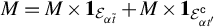 $M=M\times \textbf {1}_{\mathcal {E}_{\alpha \tilde {t}}} + M \times \textbf {1}_{\mathcal {E}_{\alpha t'}^{\mathsf {c}}}$
. Given our assumptions about the convergence of
$M=M\times \textbf {1}_{\mathcal {E}_{\alpha \tilde {t}}} + M \times \textbf {1}_{\mathcal {E}_{\alpha t'}^{\mathsf {c}}}$
. Given our assumptions about the convergence of
 $\phi _t$
, we know that for any
$\phi _t$
, we know that for any
 $\alpha>0$
and some
$\alpha>0$
and some
 $t'$
high enough, we have
$t'$
high enough, we have
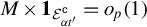 $M \times \textbf {1}_{\mathcal {E}_{\alpha t'}^{\mathsf {c}}}=o_p(1)$
. Furthermore, by Lemma A5, by choosing
$M \times \textbf {1}_{\mathcal {E}_{\alpha t'}^{\mathsf {c}}}=o_p(1)$
. Furthermore, by Lemma A5, by choosing
 $\alpha $
low enough, we see that there exists
$\alpha $
low enough, we see that there exists
 $Q^\star \in \mathcal {Q}^\star $
such that
$Q^\star \in \mathcal {Q}^\star $
such that
 $$ \begin{align*} M\times \textbf{1}_{\mathcal{E}_{\alpha t'}}&=\bigg[\sum_{m=0}^{t-t'} \bigg((I-\eta \hat{\Sigma}_X)Q^\star\bigg)^m + \sum_{m=t-t'+1}^{t-1} \prod_{l=1}^m (I-\eta \hat{\Sigma}_X)Q_{t-l}\bigg]\times \textbf{1}_{\mathcal{E}_{\alpha t'}}{.} \end{align*} $$
By Lemma A5 and dealing with indices, the right-hand side can be rewritten as
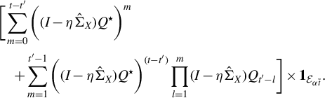 $$ \begin{align*} & \bigg[\sum_{m=0}^{t-t'} \bigg((I-\eta \hat{\Sigma}_X)Q^\star\bigg)^m \\ &\quad+ \sum_{m=1}^{t'-1} \bigg((I-\eta \hat{\Sigma}_X)Q^\star\bigg)^{(t-t')}\prod_{l=1}^m (I-\eta \hat{\Sigma}_X)Q_{t'-l}\bigg]\times \textbf{1}_{\mathcal{E}_{\alpha \tilde{t}}}. \end{align*} $$
Since by submutiplicativity of the spectral norm and Lemma A1
 $\|(I-\eta \hat {\Sigma }_X)Q^\star \|_{\mathrm {spec}}\leq \|(I-\eta \hat {\Sigma }_X)P^\star \|_{\mathrm {spec}} <1$
, we have (geometric series) that
$\|(I-\eta \hat {\Sigma }_X)Q^\star \|_{\mathrm {spec}}\leq \|(I-\eta \hat {\Sigma }_X)P^\star \|_{\mathrm {spec}} <1$
, we have (geometric series) that
 $$ \begin{align*} \sum_{l=0}^{t-t'} \bigg((I-\eta \hat{\Sigma}_X)Q^\star\bigg)^m= [(I-Q^\star)+\eta\hat{\Sigma}_X Q^\star]^{-1}[(I-\bigg((I-\eta \hat{\Sigma}_X)Q^\star\bigg)^{t-t'}]. \end{align*} $$
Moreover,
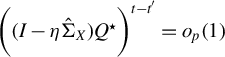 $\bigg ((I-\eta \hat {\Sigma }_X)Q^\star \bigg )^{t-t'}=o_p(1)$
and
$\bigg ((I-\eta \hat {\Sigma }_X)Q^\star \bigg )^{t-t'}=o_p(1)$
and
 $$ \begin{align*} \sum_{m=0}^{t'} \bigg((I-\eta \hat{\Sigma}_X)Q^\star\bigg)^{t-t'}\prod_{l=0}^m (I-\eta \hat{\Sigma}_X)Q_{t'-l}=o_p(1) \end{align*} $$
since
 $t-t'\rightarrow \infty $
as
$t-t'\rightarrow \infty $
as
 $n\rightarrow \infty $
. Hence, we have shown that
$n\rightarrow \infty $
. Hence, we have shown that
 $$ \begin{align*} L&=M+o_p(1)=[(I-Q^\star)+\eta\hat{\Sigma}_X Q^\star]^{-1}+o_p(1), \end{align*} $$
which is what we needed to prove.
A.9 Proof of Theorem 3
A.9.1 Lemmas
Lemma A6. Under the same set of assumptions as in Theorem 3, we have
 $\|\phi _t-\tilde {\phi }_t\|_{2}=o_p(1).$
Proof. The proof is given in the Supplementary Material.
Lemma A7. Under the same set of assumptions as in Theorem 3 (and, in particular, if
 $\inf _{\|v\|_2=1,\|v\|_0=k}|v^\top \Sigma _{XY}|>0$
and by the definition of
$\inf _{\|v\|_2=1,\|v\|_0=k}|v^\top \Sigma _{XY}|>0$
and by the definition of
 $\tilde {\phi }),$
we have
$\tilde {\phi }),$
we have
 $\sup _{t\in \{1,\ldots ,t(n)\}}\|\phi _t-\tilde {\phi }_t\|_{2}=O_p(1)$
.
$\sup _{t\in \{1,\ldots ,t(n)\}}\|\phi _t-\tilde {\phi }_t\|_{2}=O_p(1)$
.
Proof. The proof is given in the Supplementary Material.
A.9.2 Proof of Theorem 3
For the remainder of the proof, we consider that
 $\eta $
is such that
$\eta $
is such that
 $ \|(I_{p\times p}- \eta \hat {\Sigma }_X)P_t\|_{\text {spec}}<1 \text { a.s.}$
is conditional on X. The existence of
$ \|(I_{p\times p}- \eta \hat {\Sigma }_X)P_t\|_{\text {spec}}<1 \text { a.s.}$
is conditional on X. The existence of
 $\eta $
follows from Lemma A1.
$\eta $
follows from Lemma A1.
By Proposition A4, we have for all
 $t\geq 2,$
 $$ \begin{align} \phi_t-\phi^\star= \bigg( \prod_{m=1}^t (I_{p\times p} - \eta \hat{\Sigma}_X)Q_{t-m}\bigg) \phi_0 \end{align} $$
 $$ \begin{align} + \sum_{m=0}^{t-1} \bigg( \prod_{l=1}^m(I_{p\times p} - \eta \hat{\Sigma}_X)Q_{t-l}\bigg)(\phi_{t-l}-\tilde{\phi}_{t-l}) \end{align} $$
 $$ \begin{align} + \eta \sum_{m=0}^{t-1} \bigg( \prod_{l=1}^m(I_{p\times p} - \eta \hat{\Sigma}_X)Q_{t-l}\bigg) g_{t-1-m} \bigg( \hat{\Sigma}_X \phi^\star + \frac{X^\top U}{\| \beta\|_{2}n}\bigg) - \phi^\star, \end{align} $$
where
 $$ \begin{align*} g_{t-1-m}=\frac{\phi_{t-1-m}^\top \hat{\Sigma}_X \phi_{t-1-m}}{\phi_{t-1-m}^\top \hat{\Sigma}_X \phi^\star + \phi_{t-1-m}^\top \frac{X^\top U}{\|\beta\|_{2}n}}. \end{align*} $$
We treat the term on the right-hand side of (A.5). By the Cauchy–Schwarz inequality, we have
 $$ \begin{align*} \sqrt{n} w^\top\bigg( \prod_{k=1}^t (I_{p\times p} - \eta \hat{\Sigma}_X)Q_{t-k}\bigg) \phi_0 &\leq \sqrt{n} \|\bigg( \prod_{k=1}^t (I_{p\times p} - \eta \hat{\Sigma}_X)Q_{t-k}\bigg) \phi_0\|_{2} \\ &\leq \sqrt{n}\prod_{m=1}^t \| (I_{p\times p} - \eta \hat{\Sigma}_X)Q_{t-m}\|_{\mathrm{spec}} \\ &\leq \sqrt{n}\prod_{m=1}^t \| (I_{p\times p} - \eta \hat{\Sigma}_X)P_{t-m}\|_{\mathrm{spec}} \|P_{t-m}\|_{\mathrm{spec}} \\ & \leq \sqrt{n}\sup_{m\in \{1,\ldots,t\}} \| (I_{p\times p} - \eta \hat{\Sigma}_X)P_{t-m}\|_{\mathrm{spec}}^t \end{align*} $$
and by Lemma A1,
 $$ \begin{align*} \mathbb{P}\bigg( \lim_{n\rightarrow \infty} \sqrt{n} \sup_{m\in \{1,\ldots,t\}} \| (I_{p\times p} - \eta \hat{\Sigma}_X)P_{t-m}\|_{\mathrm{spec}}^t=0 \bigg|X\bigg)=1. \end{align*} $$
Now, we treat the terms (A.6). Lemmas A4, A6, and A7 ensure that by Proposition A3, conditionally on
 $X,$
we have
$X,$
we have
 $$ \begin{align*} \sum_{m=0}^{t-1} \bigg( \prod_{l=1}^m(I_{p\times p} - \eta \hat{\Sigma}_X)Q_{t-l}\bigg)(\phi_{t-l}-\tilde{\phi}_{t-l})=o_p(1). \end{align*} $$
We now treat the term (A.7). First, consider the following:
 $$ \begin{align*} \eta \sum_{m=0}^{t-1} \bigg( \prod_{l=1}^m(I_{p\times p} - \eta \hat{\Sigma}_X)Q_{t-l}\bigg) g_{t-1-m} \hat{\Sigma}_X \phi^\star -\phi^\star. \end{align*} $$
Since
 $ (I-Q^\star )\phi ^\star =0,$
we can write
$ (I-Q^\star )\phi ^\star =0,$
we can write
 $$ \begin{align*} \bigg[ \bigg(\sum_{m=0}^{t-1} \bigg( \prod_{l=1}^m(I_{p\times p} - \eta \hat{\Sigma}_X)Q_{t-l}\bigg) g_{t-1-m}) \big( (I_{p\times p}-Q^\star)+\eta\hat{\Sigma}_XQ^\star \big) -I_{p \times p} \bigg]\phi^\star. \end{align*} $$
Then, by Proposition A5, we have that this quantity converges to zero in probability conditionally on X. Finally, Proposition A5, Slutsky’s Lemma, and the CLT imply that
 $$ \begin{align*} w^\top\eta \sum_{m=0}^{t-1} \bigg( \prod_{l=1}^m(I_{p\times p} - \eta \hat{\Sigma}_X)Q_{t-l}\bigg) g_{t-1-m} \frac{X^\top U}{\| \beta\|_{2}\sqrt{n}} \end{align*} $$
is
 $$ \begin{align*} \mathcal{AN}\bigg(0,w^\top [(I-Q^\star)+\eta\hat{\Sigma}_X Q^\star]^{-1} \eta^2\hat{\Sigma}_X[(I-Q^\star)+\eta\hat{\Sigma}_X Q^\star]^{-1} w \frac{\mathbb{V}\text{ar}(U_1)}{\|\beta\|_{2}^2}\bigg|X\bigg) \end{align*} $$
hence we have proven the thesis.
B NOTATIONAL GLOSSARY
-
HD High-dimensional.
-
GEP Generalized eigenvalue problem.
-
RIFLE Truncated Rayleigh Flow Method introduced by Tan et al. (Reference Tan, Wang, Liu and Zhang2018), referred to as Algorithm 2 in this article.
-
Loaded-RIFLE Modified version of RIFLE introduced in this article and referred to as Algorithm 1.
-
(two-stage) IHT (Two-stage) iterative hard thresholding algorithm described in Jain et al. (Reference Jain, Tewari, Kar, Ghahramani, Welling, Cortes, Lawrence and Weinberger2014).
-
SDAR Support detection and root finding, algorithm introduced in Huang et al. (Reference Huang, Jiao, Liu and Lu2018)
-
$\beta $
parameter of interest
$\in \mathbb {R}^p$
.
-
$\phi ^\star $
direction of the parameter of interest, i.e.,
$\phi ^\star :=\beta /\|\beta \|_2$
.
-
$\Sigma _X:=\mathbb {E}(X_1X_1^\top ) \in \mathbb {R}^{p\times p}$
,
$\hat {\Sigma }_X:= X^\top X/n \in \mathbb {R}^{p\times p}$
,
$\Sigma _{XY}:=\mathbb {E} (X_1Y_1) \in \mathbb {R}^{p}$
,
$\hat {\Sigma }_{XY}:= X^\top Y/n \in \mathbb {R}^{p}$
, some moments of
$X_1$
and
$Y_1$
and their estimators.
-
$\rho (Z,k):=\sup _{\|v\|_{2}=1, \|v\|_0\leq k} |v^\top Z v|$
with
$Z\in \mathbb {R}^{p\times p}$
and
$k\in \mathbb {N}$
s.t.
$k\leq p$
, some norm of the matrix Z for a given k.
-
$\mathcal {F}(p,k):=\{ F\subset \{1,\ldots ,p\}; \mathrm {Card}(F)=k\}$
, for any
$k\in \mathbb {N}$
such that
$k\leq p$
, the set of sets containing k different integers between
$1$
and p.
-
$\mathcal {P}\big (\mathcal {F}(p,k)\big )$
, that is, the set of orthogonal projectors from
$\mathbb {R}^p$
to its k-dimensional subspaces that are spanned by the subsets of
$\{e_1,\ldots ,e_p\}$
whose cardinalities equal k and that preserve the order of the indexes.
-
For any
$m \in \mathbb {N}$
and
$Z\in \mathbb {R}^{m\times m}$
,
$\lambda _{\mathrm {max}}(Z), \lambda _{\mathrm {min}}(Z), \text { and } \lambda _i(Z)$
are, respectively, the maximum, minimum, and
$i^{th}$
(in descending order) eigenvalues of Z. If Z is positive definite,
$\kappa (Z) = \lambda _{\mathrm {max}}(Z) / \lambda _{\mathrm {min}}(Z)$
is the condition number of Z. -
For any
$k\in \mathbb {N}$
s.t.
$k\leq p$
and any
$F\in \mathcal {F}(k,p)$
,
$\lambda _i$
,
$\lambda _i(F)$
,
$\hat {\lambda }_i$
, and
$\hat {\lambda }_i(F)$
are the
$i^{th}$
(in descending order) generalized eigenvalues of, respectively, the pairs of matrices
$\big (\Sigma _{XY}\Sigma _{YX}, \Sigma _X \big )$
,
$\big (P_{(F)}^\top \Sigma _{XY}\Sigma _{YX}P_{(F)}$
,
$P_{(F)}^\top \Sigma _X P_{(F)} \big )$
,
$\big (\hat {\Sigma }_{XY}\hat {\Sigma }_{YX}, \hat {\Sigma }_X\big ),$
and finally
$\big (P_{(F)}^\top \hat {\Sigma }_{XY}\hat {\Sigma }_{YX} P_{(F)}, P_{(F)}^\top \hat {\Sigma }_X P_{(F)} \big )$
. -
$Cr(A,B)=\min _{\|v\|_2=1}\bigg ( \big (v^\top A v\big )^2 + \big (v^\top B v )^2\bigg )^{1/2}$
is the Crawford number of
$(A,B)$
for any
$p\in \mathbb {N}$
and any symmetric matrices
$A,B \in \mathbb {R}^{p\times p}$
.
-
$\Delta (k):= \inf _{P\in \{\cup _{i=1}^k \mathcal {P}(\mathcal {F}(p,i))\}} Cr(P^\top \Sigma _{XY}\Sigma _{YX} P, P^\top \Sigma _X P )$
for any
$k\in \mathbb {N}$
such that
$k\leq p$
.
-
$\varepsilon (k):= \bigg ( \rho (\hat {\Sigma }_{XY}\hat {\Sigma }_{YX}-\Sigma _{XY}\Sigma _{YX},k)^2 + \rho (\hat {\Sigma }_X-\Sigma _X,k)^2 \bigg )^{1/2}$
for any
$k\in \mathbb {N}$
such that
$k\leq p$
.
-
The input of Algorithm 1 is: initial vector
$ \phi _0 $
; initial and final sparsity levels
$ \overline {k}, \underline {k} \in \{1, \dots , p\} $
with
$ \overline {k}> \underline {k} $
; step size
$ \eta $
; and number of iterations
$ T $
. -
$\hat {\phi }(t)$
is the output of Algorithm 1.
-
$\mathcal {Q}^\star :=\{Q=PP^\top | P\in \cup _{i=\|\phi \|_0}^k \mathcal {P}\big (\mathcal {F}(p,i)\big ), Q\phi ^\star =\phi ^\star \}$
, a set of matrices identifying the support of
$\phi ^\star $
.


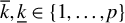


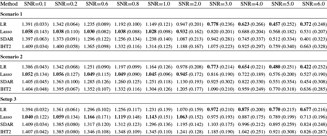


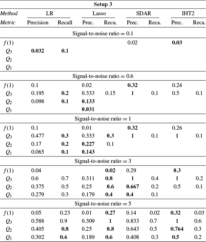


 Open access