





Impact Statement
Haemodialysis cleans blood outside the body and relies on an arteriovenous fistula to provide reliable vascular access. During treatment, repeated needle insertion for blood drainage and return substantially alters local haemodynamics, potentially creating non-physiological flow conditions and stresses that increase the risk of complications. This study delivers new fundamental insight into the flow environment by showing how needle angle and flow rate ratio govern primary and secondary flow structures, mixing pathways, and the unsteady shear stresses that develop downstream of a venous needle. While secondary flow structures have long been implicated in the development of stenosis in fistulas, we identify the mechanisms and specific regions where such structures form under controlled, clinically relevant conditions. These findings underscore the highly transient and multi-dimensional nature of needle-driven flow in fistulas. Beyond advancing the fundamental understanding of haemodynamics, this work supplies high-quality experimental data that may help refine clinical strategies for needle placement.
1. Introduction
Chronic kidney disease (CKD) often leads to end-stage renal disease (ESRD), where the kidneys do not function adequately to sustain life. In such cases, dialysis becomes essential to perform the filtration function of the kidneys. There are two main types of dialysis: haemodialysis and peritoneal dialysis. Haemodialysis removes waste and excess fluid from the blood using a machine external to the body, while peritoneal dialysis uses the lining of the abdomen as a natural filter through which dialysate absorbs waste from the bloodstream. The majority of patients on dialysis are offered haemodialysis (Johansen et al. Reference Johansen, Gilbertson, Li, Li, Liu, Roetker, Ku, Schulman, Greer, Chan, Abbott, Butler, O’Hare, Powe, Reddy, Snyder, St. Peter, Taylor, Weinhandl and Wetmore2023). Vascular access is a critical component of haemodialysis, providing a reliable and repeated entry point into the bloodstream so that blood can be efficiently removed, filtered and returned to the body. The three main types of vascular access are arteriovenous fistula (AVF), arteriovenous graft (AVG) and central venous catheter (CVC). Among these, the AVF is the most preferred access due to its superior long-term patency, lower risk of infection and fewer complications (Soleymanian et al. Reference Soleymanian, Sheikh, Tareh, Argani and Ossareh2017). AVF is a surgical connection between an artery and a vein, usually in the arm, to create a reliable high-flow access site for haemodialysis. Once the surgical creation is formed, AVF requires a maturation period during which the vein undergoes structural changes, known as ‘arterialisation’. An AVF is considered functional when it meets specific criteria, such as having a blood flow rate greater than 600 mL min−1 and a vein diameter of at least 6 mm (Hakim et al. Reference Hakim, Brooke, Beckstrom, Sarfati and Kraiss2022; Santoro et al. Reference Santoro, Benedetto, Mondello, Pipitò, Barillà, Spinelli, Ricciardi, Cernaro and Buemi2014). Once the vein matures, haemodialysis is typically performed three to four times a week. An arterial needle withdraws blood from the vein and a venous needle returns the cleaned or filtered blood.
Despite their popularity, AVFs have high failure rates, where the primary mode of failure is venous stenosis, due to intimal hyperplasia (IH) (Roy-Chaudhury et al. Reference Roy-Chaudhury, Arend, Zhang, Krishnamoorthy, Wang, Banerjee, Samaha and Munda2007; Cunnane et al. Reference Cunnane, Cunnane and Walsh2017). IH is the thickening of the inner layer of a blood vessel when cells grow and build up in response to injury or stress, and can lead to narrowing or blockage of the vessel over time. It is widely recognised that IH can develop as a result of damage to the blood vessel from surgery, repeated needle punctures for dialysis and the stress from abnormal blood flow (Lee & Roy-Chaudhury Reference Lee and Roy-Chaudhury2009; Roy-Chaudhury et al. Reference Roy-Chaudhury, Kelly, Zhang, Narayana, Desai, Melhem, Duncan and Heffelfinger2003). Specifically, IH is attributed to high or low/oscillating wall shear stress, albeit without a consensus and a significant body of research supporting both (Cunnane et al. Reference Cunnane, Cunnane and Walsh2017). Further, quantitative flow parameters such as turbulent disturbances and perivascular vibrations have been associated as factors responsible for the development of IH (Unnikrishnan et al. Reference Unnikrishnan, Huynh, Brott, Ito, Cheng, Shih, Allon and Anayiotos2005), and stenosis is a direct consequence of IH (Bilgic et al. Reference Bilgic, Yilmaz, Bozkurt, Celik, Bilgic, Gurel, Kirbas, Bavbek and Akcay2015; Turmel-Rodrigues et al. Reference Turmel-Rodrigues, Pengloan, Baudin, Testou, Abaza, Dahdah, Mouton and Blanchard2000). These observations highlight the importance of examining the detailed fluid dynamics in AVFs to better understand and identify potential failure mechanisms.
Two critical regions of interest are the flow patterns near the anastomosis, where the artery and vein are surgically connected, and the localised flow disturbances that occur during repeated needling for dialysis access. While focusing on the fluid flow near the anastomosis region, the influence of anastomosis angle (Cunnane et al. Reference Cunnane, Cunnane, Moran and Walsh2019; Park et al. Reference Park, Song, Kim, Kim, Kim and Lee2016), distribution of flow rate in the artery and the vein (Sivanesan et al. 1999), wall compliance, and effect of pulsatile flow in the artery (Alam & Newport Reference Alam and Newport2022; Browne et al. Reference Browne, Walsh and Griffin2015; Decorato et al. Reference Decorato, Kharboutly, Vassallo, Penrose, Legallais and Salsac2014) are well studied. Further, many studies also focused on patient-specific geometries (Bartlett et al. Reference Bartlett, Bonfanti, Diaz-Zuccarini and Tsui2024; Bozzetto et al. Reference Bozzetto, Ene-Iordache and Remuzzi2016; Cunnane et al. Reference Cunnane, Cunnane, Moran and Walsh2019; Ene-Iordache et al. Reference Ene-Iordache, Mosconi, Remuzzi and Remuzzi2001; Gunasekera et al. Reference Gunasekera, Ng, Thomas, Varcoe, De Silva and Barber2020). Notably, there is a significantly greater body of research focused on flow dynamics at the anastomosis (Drost et al. Reference Drost, Alam, Houston and Newport2017; McCullough & Coveney Reference McCullough and Coveney2021; Wang et al. Reference Wang, Wang, Guo, Zhang, Mu and Liu2024), while studies that examine the haemodynamic effects of needling remain relatively limited (Borg & Fuchs Reference Borg and Fuchs2002; Unnikrishnan et al. Reference Unnikrishnan, Huynh, Brott, Ito, Cheng, Shih, Allon and Anayiotos2005, Fulker et al. Reference Fulker, Simmons, Kabir, Kark and Barber2016, Reference Fulker, Forster, Simmons and Barber2017 Reference Fulker, Forster, Simmons and Barbera , Reference Fulker, Simmons and Barberb ; Woraratsoontorn & Bunmun Reference Woraratsoontorn and Bunmun2024).
The needling process in AVFs shares similarities with the classical fluid dynamics problem of a jet in an elevated cross-flow (Gupta & Saha Reference Gupta and Saha2024) and, more specifically, an oblique jet impacting in a submerged environment (Mishra et al. Reference Mishra, Yadav, Djenidi and Agrawal2020; Wang et al. Reference Wang, Wang, Shi, Lu, Tan and Zhou2017). However, due to the geometric constriction in the form of a circular vein and the high jet-to-co-flow velocity and momentum flux ratios, the flow environment in AVFs is significantly more complex, These factors may strongly influence shear stress distribution, flow separation and downstream disturbances, factors critical to understanding vascular injury and remodelling (Marticorena & Donnelly Reference Marticorena and Donnelly2016). Indeed, in an in vitro haemodialysis model, turbulent flow created by the haemodialysis needle was shown to inhibit nitric oxide (NO) formation and loss of endothelial cell integrity (Huynh et al. Reference Huynh, Chacko, Teng, Brott, Allon, Kelpke, Thompson, Patel and Anayiotos2007). This loss of NO signalling may lead to IH formation during haemodialysis. An earlier study showed the influence of such venous needle flow in an idealised geometry of AVF, by experimentally visualising the transport of a scalar using planar laser-induced fluorescence (PLIF) (Borg & Fuchs Reference Borg and Fuchs2002). High fluctuations in the concentration of the substance coming from the venous flow were observed near the vein wall for long distances downstream of the needle (Borg & Fuchs Reference Borg and Fuchs2002). Regarding needle-induced turbulence in an AVG, it was later reported that the generated turbulence intensity is 5–6 times higher compared with the case of no needle (Unnikrishnan et al. Reference Unnikrishnan, Huynh, Brott, Ito, Cheng, Shih, Allon and Anayiotos2005). Several studies have used computational fluid dynamics (CFD) to study the fluid flow during needling in AVF. In an idealised version of the cephalic vein as a pipe, the effect of needle rotation was studied for both the venous needle and the arterial needle (Fulker et al. Reference Fulker, Simmons, Kabir, Kark and Barber2016). The authors concluded that there is no haemodynamic benefit in rotating the needle in achieving reduced wall shear stress (WSS) and smooth flow without oscillatory motion. This is similar to the conclusion from another recent study (Woraratsoontorn & Bunmun Reference Woraratsoontorn and Bunmun2024). Following this, a more complex scenario of both arterial and venous needles simultaneously, in a patient-specific geometry was investigated (Fulker et al. Reference Fulker, Simmons and Barber2017 Reference Fulker, Simmons and Barberb ). Experimentally, using stereoscopic particle image velocimetry (PIV), the velocity field in a geometrically 1:2 scaled and idealised AVF has been previously reported. The authors reported a secondary flow structure resulting from the interaction between the jet flow from the needle and the flow in the vein, consistent with varying flow rates and needle angles (Fulker et al. Reference Fulker, Forster, Simmons and Barber2017 Reference Fulker, Forster, Simmons and Barbera ). The present work extends this understanding by complementing mean flow analysis with PLIF-based visualisation of scalar transport and a PIV-derived quantification of temporal shear-stress fluctuations, together with a detailed characterisation of the unsteady flow field, aspects not addressed in prior experimental work (Fulker et al. Reference Fulker, Forster, Simmons and Barber2017 Reference Fulker, Forster, Simmons and Barbera ).
Evidently, experimental work on studying the fluid flow during needling remains sparse. Hypothesising that the unsteadiness of the flow, resulting in highly dynamic stress characteristics and distinct flow regions, directly influences the risks of complications in AVF, our aim was to experimentally investigate the fundamental aspects of fluid flow in simpler and idealised scenarios using PLIF and PIV. We reduced the complexity of the vascular access in AVF to study only the venous needle part of the problem, where the cleaned blood is returned to the system. We used an idealised geometry where the dimensions of the venous vessel and the needle closely match those commonly encountered in practice. Flow rates were scaled to match Reynolds numbers observed in vivo, ensuring dynamic similarity while working with water for the experiments. The study systematically varied two key parameters: the flow rate ratio (venous flow rate to needle flow rate) and the angle of needle insertion relative to the vein axis. Particular emphasis was placed on the role of shear stress as a key fluid-dynamic factor by examining both transient and mean values.
2. Experimental methods
2.1. Experimental set-up
A schematic of the experimental set-up is shown in Figure 1. The vein was modelled as a straight circular pipe with an inner diameter (ID) of $D_v= 8$
mm and an outer diameter (OD) of 12 mm, made of clear PMMA (Nordbergs Tekniska; Sweden). The venous needle was idealised as a smaller pipe with an ID of
$D_v= 8$
mm and an outer diameter (OD) of 12 mm, made of clear PMMA (Nordbergs Tekniska; Sweden). The venous needle was idealised as a smaller pipe with an ID of $d= 1.6$
mm and an OD of 2 mm, made of stainless steel (G.Kinnvall AB; Sweden). The vein dimensions were chosen according to the average diameter of a matured vein post arterialisation in the AVF (6–12 mm). The needle dimensions correspond closely to a 14G dialysis needle (Ahn et al. Reference Ahn, Bahk and Lim2002). To guarantee fully developed and stationary inflow conditions, the lengths of both the vein and venous needle were set to more than 50 times their respective diameters, prior to the region of interest where the flows converge, as shown in a red rectangle in Figure 1. For the vein flow, the fully developed velocity profile was experimentally verified and subsequently used to assess the methodological uncertainty (see § 2.3). The downstream portion of the vein had a length of 30 times the diameter to prevent any backflow from the outlet affecting the flow in the region of interest. The flow system included three independent head tanks: one containing water seeded with tracer particles for velocity measurements, one with dyed water for scalar transport studies and one with clear water. The flow loop was designed to selectively supply any of these fluids to either the vein or the needle, depending on the measurement technique being employed. For PIV, the outlet from the vein was directly connected back to the head tank, resulting in a closed-loop system. For PLIF, the mixed water at the outlet of the vein could not be reused and, hence, the outlet was connected to waste. Care was taken to maintain a constant fluid level in the head tanks by using a secondary supply tank and a level-control arrangement. The water temperature during all experiments was measured to be
$d= 1.6$
mm and an OD of 2 mm, made of stainless steel (G.Kinnvall AB; Sweden). The vein dimensions were chosen according to the average diameter of a matured vein post arterialisation in the AVF (6–12 mm). The needle dimensions correspond closely to a 14G dialysis needle (Ahn et al. Reference Ahn, Bahk and Lim2002). To guarantee fully developed and stationary inflow conditions, the lengths of both the vein and venous needle were set to more than 50 times their respective diameters, prior to the region of interest where the flows converge, as shown in a red rectangle in Figure 1. For the vein flow, the fully developed velocity profile was experimentally verified and subsequently used to assess the methodological uncertainty (see § 2.3). The downstream portion of the vein had a length of 30 times the diameter to prevent any backflow from the outlet affecting the flow in the region of interest. The flow system included three independent head tanks: one containing water seeded with tracer particles for velocity measurements, one with dyed water for scalar transport studies and one with clear water. The flow loop was designed to selectively supply any of these fluids to either the vein or the needle, depending on the measurement technique being employed. For PIV, the outlet from the vein was directly connected back to the head tank, resulting in a closed-loop system. For PLIF, the mixed water at the outlet of the vein could not be reused and, hence, the outlet was connected to waste. Care was taken to maintain a constant fluid level in the head tanks by using a secondary supply tank and a level-control arrangement. The water temperature during all experiments was measured to be $23 \pm 2\,^{\circ }\text{C}$
. The needle was inserted into the vein through a precisely drilled hole and securely fixed in place using acrylic adhesive (Acrifix 1R 0192). Centrifugal blood pumps were used to maintain the flow in the vein (CenteriMag; Abbott Laboratories, US) and the needle (Rotaflow; Getinge AB, Sweden). The flow rates were measured by two separate ultrasonic flow meters (VMI02; SIKA, Kaufungen, Germany). The whole of the vein was enclosed in an acrylic chamber filled with water to minimise optical errors due to refraction at a solid–fluid interface.
$23 \pm 2\,^{\circ }\text{C}$
. The needle was inserted into the vein through a precisely drilled hole and securely fixed in place using acrylic adhesive (Acrifix 1R 0192). Centrifugal blood pumps were used to maintain the flow in the vein (CenteriMag; Abbott Laboratories, US) and the needle (Rotaflow; Getinge AB, Sweden). The flow rates were measured by two separate ultrasonic flow meters (VMI02; SIKA, Kaufungen, Germany). The whole of the vein was enclosed in an acrylic chamber filled with water to minimise optical errors due to refraction at a solid–fluid interface.
Schematic of the experimental set-up. Inset in the red rectangle shows representative images of raw data acquired from PLIF and PIV.

2.2. Methodology
PLIF and PIV experiments were performed primarily in a central longitudinal plane of the vein (plane $(x,y)$
in Figure 1), extending from the needle exit to ca. 45 mm downstream. To complement these measurements, additional PIV experiments were carried out in the transverse streamwise-spanwise plane (
$(x,y)$
in Figure 1), extending from the needle exit to ca. 45 mm downstream. To complement these measurements, additional PIV experiments were carried out in the transverse streamwise-spanwise plane ( $(x,z)$
plane). The
$(x,z)$
plane). The $(x,y)$
plane forms the basis of the results presented in this work, while selected
$(x,y)$
plane forms the basis of the results presented in this work, while selected $(x,z)$
-plane measurements are included to further complement the results from the
$(x,z)$
-plane measurements are included to further complement the results from the $(x,y)$
plane.
$(x,y)$
plane.
For PLIF, Rhodamine B (RhB) was used as the fluorescent dye, introduced only through the needle flow, while the vein flow remained undyed during measurements. A Litron LPY703 Nd:YAG laser was used to illuminate the plane, with a thin laser sheet formed using a Focus Module (Dantec Dynamics, Denmark). The fluorescence signal was recorded with a FlowSense camera (Dantec Dynamics) fitted with a Nikon 50 mm lens and an OG570 long-pass optical filter (Schott, USA), blocking the laser wavelength and transmitting only the dye emission. For PLIF calibration, both the vein and needle streams were continuously supplied with Rhodamine B solutions at concentrations ranging from 0 to 50 $\unicode{x03BC}$
g L−1, for a fixed laser intensity. Within this range, the fluorescence intensity exhibited a linear dependence on dye concentration. In the experiments, only the needle flow was dyed, using a RhB concentration of 25
$\unicode{x03BC}$
g L−1, for a fixed laser intensity. Within this range, the fluorescence intensity exhibited a linear dependence on dye concentration. In the experiments, only the needle flow was dyed, using a RhB concentration of 25 $\unicode{x03BC}$
g L−1, while the vein flow remained undyed. The calibration and data analysis in the experimental runs were performed using Dynamic Studio (Dantec Dynamics).
$\unicode{x03BC}$
g L−1, while the vein flow remained undyed. The calibration and data analysis in the experimental runs were performed using Dynamic Studio (Dantec Dynamics).
PIV measurements were carried out using the same laser operated in double-frame mode, with a 100 $\unicode{x03BC}$
s duration between the two frames. The working fluid was seeded with hollow glass spheres (LaVision, Germany) as tracer particles. The same FlowSense camera and 50 mm lens, this time without the long-pass filter, were used to capture particle images. All measurements were recorded at a frequency of 50 Hz with a spatial resolution of 17.04
$\unicode{x03BC}$
s duration between the two frames. The working fluid was seeded with hollow glass spheres (LaVision, Germany) as tracer particles. The same FlowSense camera and 50 mm lens, this time without the long-pass filter, were used to capture particle images. All measurements were recorded at a frequency of 50 Hz with a spatial resolution of 17.04 $\unicode{x03BC}$
m pixels−1. The PIV images were processed in Dynamic Studio, using an adaptive multi-pass cross-correlation algorithm, starting with interrogation windows of 64 × 64 pixels and refining to 32 × 32 pixels, with a grid step size of 16 × 16 pixels. The interrogation window size was adaptively adjusted to account for local velocity gradients, and a validation filter with a peak-height ratio threshold of 1.2 was applied to eliminate spurious vectors. After validation, erroneous vectors were substituted using interpolation, with substituted vectors accounting for less than 2.5 % of the total.
$\unicode{x03BC}$
m pixels−1. The PIV images were processed in Dynamic Studio, using an adaptive multi-pass cross-correlation algorithm, starting with interrogation windows of 64 × 64 pixels and refining to 32 × 32 pixels, with a grid step size of 16 × 16 pixels. The interrogation window size was adaptively adjusted to account for local velocity gradients, and a validation filter with a peak-height ratio threshold of 1.2 was applied to eliminate spurious vectors. After validation, erroneous vectors were substituted using interpolation, with substituted vectors accounting for less than 2.5 % of the total.
For each experimental run, a total of 1000 images (corresponding to 20 s) were acquired for both PLIF and PIV measurements, with each image providing a single data set representing the instantaneous flow field. The mean results presented in this study were obtained by averaging over these 1000 instantaneous data sets.
Table 1 summarises the operating conditions considered in the present study. Two parameters were systematically varied: the flow rate ratio, $Q = Q_v/Q_n$
, and the needle angle,
$Q = Q_v/Q_n$
, and the needle angle, $\theta$
. The flow rate in the vein,
$\theta$
. The flow rate in the vein, $Q_v$
, was either 200 or 300 mL min−1, together with the flow rate in the needle,
$Q_v$
, was either 200 or 300 mL min−1, together with the flow rate in the needle, $Q_n$
, at 100 or 200 mL min−1, giving flow rate ratios in the range
$Q_n$
, at 100 or 200 mL min−1, giving flow rate ratios in the range $Q=3$
to
$Q=3$
to $Q=1$
. The corresponding Reynolds numbers, computed using the inner diameter and average velocity of each channel, are also reported in Table 1, along with the velocity ratio and momentum-flux ratio. The average velocity in each channel was calculated as
$Q=1$
. The corresponding Reynolds numbers, computed using the inner diameter and average velocity of each channel, are also reported in Table 1, along with the velocity ratio and momentum-flux ratio. The average velocity in each channel was calculated as $V_v= Q_v/(\pi D^2/4)$
and
$V_v= Q_v/(\pi D^2/4)$
and $V_n= Q_n/(\pi d^2/4)$
. Consequently, Reynolds numbers were calculated as
$V_n= Q_n/(\pi d^2/4)$
. Consequently, Reynolds numbers were calculated as $Re_v=\rho V_v D/\mu$
and
$Re_v=\rho V_v D/\mu$
and $Re_n=\rho V_n d/\mu$
, with
$Re_n=\rho V_n d/\mu$
, with $\rho$
=
$\rho$
= ${1000}\,\textrm {kg}\,{\textrm {m}}^{-3}$
and
${1000}\,\textrm {kg}\,{\textrm {m}}^{-3}$
and $\mu$
= 1 mPa s. To ensure dynamic similarity with clinical conditions, Reynolds numbers were matched by accounting for the fact that blood behaves nearly Newtonian at shear rates above
$\mu$
= 1 mPa s. To ensure dynamic similarity with clinical conditions, Reynolds numbers were matched by accounting for the fact that blood behaves nearly Newtonian at shear rates above $100\,\text{s}^{-1}$
, for haematocrit levels of 20 %–40 %, with an effective viscosity approximately three times that of water (Wells et al. Reference Wells and Merrill1962; Lemétayer et al., Reference Lemétayer, Broman and Prahl Wittberg2021). Assuming similarity in density of whole blood and water (whole blood is
$100\,\text{s}^{-1}$
, for haematocrit levels of 20 %–40 %, with an effective viscosity approximately three times that of water (Wells et al. Reference Wells and Merrill1962; Lemétayer et al., Reference Lemétayer, Broman and Prahl Wittberg2021). Assuming similarity in density of whole blood and water (whole blood is ${\sim}5$
% to 6 % denser than water, at 20
${\sim}5$
% to 6 % denser than water, at 20 $^\circ$
C (Trudnowski & Rico Reference Trudnowski and Rico1974)), and by maintaining similar geometric parameters, the threefold lower viscosity of water required velocities one-third of the clinical values to achieve the same Reynolds number. Accordingly, the experimental volumetric flow rates were set to one-third of the clinical representative values. As can be observed from Table 1, the
$^\circ$
C (Trudnowski & Rico Reference Trudnowski and Rico1974)), and by maintaining similar geometric parameters, the threefold lower viscosity of water required velocities one-third of the clinical values to achieve the same Reynolds number. Accordingly, the experimental volumetric flow rates were set to one-third of the clinical representative values. As can be observed from Table 1, the $Re_v$
and
$Re_v$
and $Re_n$
suggest the flow to be laminar in the vein and transitional in the needle, before the two flows mix. The laminar regime in the vein is further confirmed by the measured parabolic velocity profile, which is also used to estimate the uncertainty in the velocity measurements, as discussed in § 2.3.
$Re_n$
suggest the flow to be laminar in the vein and transitional in the needle, before the two flows mix. The laminar regime in the vein is further confirmed by the measured parabolic velocity profile, which is also used to estimate the uncertainty in the velocity measurements, as discussed in § 2.3.
Operating parameters and relevant non-dimensional numbers considered in the present study. For each flow rate ratio $Q=\frac {Q_v}{Q_n}$
, experiments were performed at needle angles of
$Q=\frac {Q_v}{Q_n}$
, experiments were performed at needle angles of $20^\circ$
,
$20^\circ$
, $40^\circ$
and
$40^\circ$
and $60^\circ$

The choice of these operating conditions was motivated by both physiological relevance and limiting fluid dynamic considerations. The case $Q=3$
(with
$Q=3$
(with $Q_v=300$
and
$Q_v=300$
and $Q_n=100$
mL min−1) closely replicates a typical clinical scenario with vein and needle flow rates of approximately 900 and 300 mL min−1, respectively. Here, it can be noted that
$Q_n=100$
mL min−1) closely replicates a typical clinical scenario with vein and needle flow rates of approximately 900 and 300 mL min−1, respectively. Here, it can be noted that $Q=3$
corresponds to a flow velocity of the needle that is approximately 17 times that of the flow velocity in the vein (
$Q=3$
corresponds to a flow velocity of the needle that is approximately 17 times that of the flow velocity in the vein ( $U_r=16.7$
in Table 1), implying that strong shear layers are developing around the exit of the needle. Ratios of
$U_r=16.7$
in Table 1), implying that strong shear layers are developing around the exit of the needle. Ratios of $Q=2$
and
$Q=2$
and $Q=1.5$
represent limiting cases of reduced vein flow and enhanced needle flow, while
$Q=1.5$
represent limiting cases of reduced vein flow and enhanced needle flow, while $Q=1$
corresponds to equal flow rates in the vein and needle, serving as a fundamental reference case. As the flow rate ratio decreases from
$Q=1$
corresponds to equal flow rates in the vein and needle, serving as a fundamental reference case. As the flow rate ratio decreases from $Q= 3$
to
$Q= 3$
to $1$
, the velocity ratio
$1$
, the velocity ratio $U_r={V_n}/{V_v}$
increases from ca. 8 to 25. In addition, the angle between the needle axis and the vein axis was varied at
$U_r={V_n}/{V_v}$
increases from ca. 8 to 25. In addition, the angle between the needle axis and the vein axis was varied at $20^\circ$
,
$20^\circ$
, $40^\circ$
and
$40^\circ$
and $60^\circ$
.
$60^\circ$
.
2.3. Uncertainty
Uncertainty in measuring the flow rate was less than $2.5\,\%$
. Measurement uncertainties in PLIF and PIV were quantified by separating systematic (
$2.5\,\%$
. Measurement uncertainties in PLIF and PIV were quantified by separating systematic ( $\epsilon _{\mathrm{sys}}$
) and random (
$\epsilon _{\mathrm{sys}}$
) and random ( $\epsilon _{\mathrm{rand}}$
) components. For PLIF,
$\epsilon _{\mathrm{rand}}$
) components. For PLIF, $\epsilon _{\mathrm{sys}}$
was assessed using a dye concentration not included in the calibration dataset; the mean deviation was approximately
$\epsilon _{\mathrm{sys}}$
was assessed using a dye concentration not included in the calibration dataset; the mean deviation was approximately $1.7\,\%$
, while the standard deviation was
$1.7\,\%$
, while the standard deviation was $10\,\%$
. The random component,
$10\,\%$
. The random component, $\epsilon _{\mathrm{rand}}$
, estimated from repeated trials, was approximately
$\epsilon _{\mathrm{rand}}$
, estimated from repeated trials, was approximately $2\,\%$
. For PIV,
$2\,\%$
. For PIV, $\epsilon _{\mathrm{sys}}$
was estimated by comparing the measured velocity profile in the vein, taken 50 diameters downstream of the inlet, with the analytical Poiseuille solution for fully developed pipe flow. The mean deviation in centreline velocity was approximately
$\epsilon _{\mathrm{sys}}$
was estimated by comparing the measured velocity profile in the vein, taken 50 diameters downstream of the inlet, with the analytical Poiseuille solution for fully developed pipe flow. The mean deviation in centreline velocity was approximately $6.5\,\%$
, with a standard deviation of approximately
$6.5\,\%$
, with a standard deviation of approximately $10\,\%$
. The corresponding
$10\,\%$
. The corresponding $\epsilon _{\mathrm{rand}}$
, obtained from repeated experiments, was approximately
$\epsilon _{\mathrm{rand}}$
, obtained from repeated experiments, was approximately $3\,\%$
of the mean velocity. In both techniques, calibration or reference-based precision was the dominant source of uncertainty, while random variability across repetitions remained comparatively small. The overall measurement uncertainty was obtained by combining the two contributions in quadrature,
$3\,\%$
of the mean velocity. In both techniques, calibration or reference-based precision was the dominant source of uncertainty, while random variability across repetitions remained comparatively small. The overall measurement uncertainty was obtained by combining the two contributions in quadrature,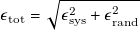 $\epsilon _{\mathrm{tot}} = \sqrt {\epsilon _{\mathrm{sys}}^{2} + \epsilon _{\mathrm{rand}}^{2}}$
, yielding approximately
$\epsilon _{\mathrm{tot}} = \sqrt {\epsilon _{\mathrm{sys}}^{2} + \epsilon _{\mathrm{rand}}^{2}}$
, yielding approximately $10\,\%$
for PLIF and
$10\,\%$
for PLIF and $12\,\%$
for PIV.
$12\,\%$
for PIV.
3. Results
First, an overview of the general flow characteristics is presented in § 3.1, starting with scalar transport and mixing, and followed by velocity fields. The influence of the flow rate ratio is examined in detail for a fixed needle angle of 40 $^\circ$
, chosen as the representative medium angle. For clarity, results are first shown for the representative case with
$^\circ$
, chosen as the representative medium angle. For clarity, results are first shown for the representative case with $Q=3$
, followed by the remaining three flow rates. Subsequently, in § 3.2, the effect of needle angle is assessed. Finally, in § 3.3, viscous shear stress (VSS), derived from the velocity data, is analysed to provide further insights into the haemodynamic environment downstream of the venous needle.
$Q=3$
, followed by the remaining three flow rates. Subsequently, in § 3.2, the effect of needle angle is assessed. Finally, in § 3.3, viscous shear stress (VSS), derived from the velocity data, is analysed to provide further insights into the haemodynamic environment downstream of the venous needle.
3.1. Flow characteristics
Figure 2
a shows raw PLIF images for the representative case of $Q=3$
(
$Q=3$
( $Q_v=300$
mL min−1,
$Q_v=300$
mL min−1, $Q_n=100$
mL min−1). Three instantaneous snapshots are presented to provide a qualitative view of the scalar field. The flow features and structures are broadly consistent across all flow rate ratios studied, and this case illustrates the fundamental characteristics observed throughout the experimental cases investigated. The needle jet emerges in a steady streamlined manner, with no large-scale vortex shedding observed immediately downstream of the needle exit. The time-resolved velocity along the jet centreline remains largely steady about a constant mean. At locations 1 and 1.5 needle diameters downstream, the ratio of root-mean-square (rms) of fluctuation to mean velocity ratios is 10 %–13 %, which is within the measurement uncertainty of the PIV system.
$Q_n=100$
mL min−1). Three instantaneous snapshots are presented to provide a qualitative view of the scalar field. The flow features and structures are broadly consistent across all flow rate ratios studied, and this case illustrates the fundamental characteristics observed throughout the experimental cases investigated. The needle jet emerges in a steady streamlined manner, with no large-scale vortex shedding observed immediately downstream of the needle exit. The time-resolved velocity along the jet centreline remains largely steady about a constant mean. At locations 1 and 1.5 needle diameters downstream, the ratio of root-mean-square (rms) of fluctuation to mean velocity ratios is 10 %–13 %, which is within the measurement uncertainty of the PIV system.
Two dominant flow structures are evident. The first is the needle jet impinging on the wall, forming a streamwise wall jet that interacts with the venous flow. Shear-layer vortices develop in the mixing layers, suggesting the flow downstream is transitional in nature with vortex shedding. These vortices originate from the Kelvin–Helmholtz instability, an inviscid instability caused due to the difference in streamwise velocity in a shear layer (Popiel & Trass Reference Popiel and Trass1991). For more details about the instability mechanism and characterisation, refer the works of Bajura & Catalano (Reference Bajura and Catalano1975), Huang & Lan (Reference Huang and Lan2005), van Hooff et al. (Reference van, Twan, Bert, Thijs and Van Heijst2012), Ilak et al. (Reference Ilak, Schlatter, Bagheri and Henningson2012), Pieris (Reference Pieris2017) and Rohlfs et al. (Reference Rohlfs, Jörg, Ehrenpreis, Rietz, Haustein and Kneer2015). A small recirculation zone is seen upstream of the area of needle jet impingement on the venous wall, consistent with previous observations of oblique jet impacts in quiescent flows (Mishra et al. Reference Mishra, Yadav, Djenidi and Agrawal2020). The second dominant flow structure is a quasi-stationary structure observed near the upper venous wall where the wall jet meets the venous flow, indicating a region of reduced velocity or recirculation. This arises from the circumferential flow along the vein wall, which merges with the wall jet downstream. This is illustrated in figure 2 b, presenting an instantaneous snapshot of the flow field, visualised using fluorescein introduced through the needle (see supplementary movie 1 available at https://doi.org/10.1017/flo.2026.10057). Representative streamlines show the two dominant flow structures. The frequency of shredding of shear layer vortices, the features of the wall jet, and the position and extent of the secondary flow structure depend on the flow rate ratio and needle angle, and are discussed in subsequent sections.
(a) Flow visualisation as raw data acquired from PLIF experiments is shown for the flow rate ratio of $Q=3$
. (b) Instantaneous snapshot of the flow, visualised using fluorescein in the needle, in an isometric view, with representative streamlines overlaid to illustrate the wall jet (primary flow structure) and the circumferential flow along the vein wall (leading to the secondary flow structure).
$Q=3$
. (b) Instantaneous snapshot of the flow, visualised using fluorescein in the needle, in an isometric view, with representative streamlines overlaid to illustrate the wall jet (primary flow structure) and the circumferential flow along the vein wall (leading to the secondary flow structure).

3.1.1. Mixing
Scalar transport is examined using the concentration of dye originating from the needle jet. To enable comparison across the flow field, the local concentration $c$
is normalised by the inlet concentration
$c$
is normalised by the inlet concentration $c_0$
at the needle, termed as mixture fraction. This mixture fraction ranges from 0 to 1, where 0 corresponds to pure venous flow, 1 to flow entirely from the needle and intermediate values indicate varying contributions from both streams, thereby reflecting the extent of mixing. The criterion for complete mixing is defined as the condition in which the two streams are fully homogenised, such that the mixture fraction attains a spatially uniform value of
$c_0$
at the needle, termed as mixture fraction. This mixture fraction ranges from 0 to 1, where 0 corresponds to pure venous flow, 1 to flow entirely from the needle and intermediate values indicate varying contributions from both streams, thereby reflecting the extent of mixing. The criterion for complete mixing is defined as the condition in which the two streams are fully homogenised, such that the mixture fraction attains a spatially uniform value of $1/(1+Q)$
across the venous cross-section, where
$1/(1+Q)$
across the venous cross-section, where $Q$
is the ratio of the venous to needle volumetric flow rates. This theoretical value follows directly from conservation of mass, given that only the needle flow is dyed: at a fully mixed state,
$Q$
is the ratio of the venous to needle volumetric flow rates. This theoretical value follows directly from conservation of mass, given that only the needle flow is dyed: at a fully mixed state, $Q_n \cdot c_0 + Q_v \cdot 0 = (Q_n + Q_v) \cdot c_{\text{mix}}$
, which gives
$Q_n \cdot c_0 + Q_v \cdot 0 = (Q_n + Q_v) \cdot c_{\text{mix}}$
, which gives $c_{\text{mix}} = Q_n c_0 / (Q_n + Q_v)$
. Normalising by
$c_{\text{mix}} = Q_n c_0 / (Q_n + Q_v)$
. Normalising by $c_0$
yields the mixture fraction as
$c_0$
yields the mixture fraction as $1/(1+Q)$
. In the following, the time-averaged mixture fraction (referred to as mean mixture fraction) and the corresponding rms fluctuation are presented as
$1/(1+Q)$
. In the following, the time-averaged mixture fraction (referred to as mean mixture fraction) and the corresponding rms fluctuation are presented as $\lt c\gt /c_{0}$
and
$\lt c\gt /c_{0}$
and $c' /c_{0}$
, respectively.
$c' /c_{0}$
, respectively.
The mean mixture fraction provides a time-averaged characterisation of the spatial distribution of the two fluid streams, identifying regions of complete, partial and negligible mixing. In the clinical context of AVF needling, where a haemodialysis session typically lasts for two to three hours, the mean field is the most relevant quantity for assessing the overall interaction between the two streams. The rms fluctuation complements this by quantifying the degree of transient unsteadiness in the scalar field; a low rms where the mean has attained $1/(1+Q)$
confirms a statistically steady mixed state, whereas a significant rms indicates dominance of organised transient structures.
$1/(1+Q)$
confirms a statistically steady mixed state, whereas a significant rms indicates dominance of organised transient structures.
For the representative case of $Q=3$
(Figure 2), the mean mixture fraction is shown in Figure 3a and the corresponding rms fluctuation is presented in Figure 3b. The mean mixture fraction clearly reflects the two primary flow structures discussed earlier and their subsequent merging. Elevated mixture fraction is observed in the quasi-stationary structure near the upper vein wall, indicating a region of low velocity or recirculation. It should be noted that concentration data immediately above the needle, for
$Q=3$
(Figure 2), the mean mixture fraction is shown in Figure 3a and the corresponding rms fluctuation is presented in Figure 3b. The mean mixture fraction clearly reflects the two primary flow structures discussed earlier and their subsequent merging. Elevated mixture fraction is observed in the quasi-stationary structure near the upper vein wall, indicating a region of low velocity or recirculation. It should be noted that concentration data immediately above the needle, for $x/d \lesssim 0$
, are not physical, as the laser sheet from below does not illuminate this region. To preserve the integrity of the experimental dataset, however, this region was not masked or deleted. It is interesting that there is a non-zero rms component (
$x/d \lesssim 0$
, are not physical, as the laser sheet from below does not illuminate this region. To preserve the integrity of the experimental dataset, however, this region was not masked or deleted. It is interesting that there is a non-zero rms component ( ${\sim}10$
% of the inlet concentration) in the normalised concentration of the needle jet before it impacts on the wall, similar to observations presented by Borg et al. (Reference Borg and Fuchs2002). This level of rms fluctuation is comparable to the systematic component,
${\sim}10$
% of the inlet concentration) in the normalised concentration of the needle jet before it impacts on the wall, similar to observations presented by Borg et al. (Reference Borg and Fuchs2002). This level of rms fluctuation is comparable to the systematic component, $\epsilon _{\mathrm{sys}}$
, as presented in § 2. Hence, although such variation could be caused by a weak swirl in the emerging jet, potentially caused by reducing connectors in the circuit (Fulker et al. Reference Fulker, Forster, Simmons and Barber2017
Reference Fulker, Forster, Simmons and Barbera
), the present rms levels fall within the range of measurement uncertainty and, therefore, cannot be attributed to any physical mechanism with confidence.
$\epsilon _{\mathrm{sys}}$
, as presented in § 2. Hence, although such variation could be caused by a weak swirl in the emerging jet, potentially caused by reducing connectors in the circuit (Fulker et al. Reference Fulker, Forster, Simmons and Barber2017
Reference Fulker, Forster, Simmons and Barbera
), the present rms levels fall within the range of measurement uncertainty and, therefore, cannot be attributed to any physical mechanism with confidence.
The rms fluctuation highlights zones of unsteadiness, with the highest fluctuations located in the shear layer where vortices develop, followed by the region near the downstream upper wall. Quantitative profiles of the mean mixture fraction and the corresponding rms values at selected downstream locations are plotted in Figures 3c and 3d, respectively. At $x/d=25$
, the mixture fraction profile across the vein remains non-uniform, indicating incomplete mixing between the two streams. The maximum rms values reach ca.
$x/d=25$
, the mixture fraction profile across the vein remains non-uniform, indicating incomplete mixing between the two streams. The maximum rms values reach ca. $0.3$
, corresponding to approximately
$0.3$
, corresponding to approximately $30\,\%$
of the inlet concentration, concentrated within the shear layer region. Further, as a result of uncertainty in measuring concentration being 10 % (see § 2.3), rms fluctuations less than 10 % are not considered statistically distinguishable from noise and are thus not physically conclusive. Nevertheless, in regions of interest such as shear layers and regions where complete mixing is not observed, the rms fluctuation exceeds this measurement uncertainty and can be analysed meaningfully.
$30\,\%$
of the inlet concentration, concentrated within the shear layer region. Further, as a result of uncertainty in measuring concentration being 10 % (see § 2.3), rms fluctuations less than 10 % are not considered statistically distinguishable from noise and are thus not physically conclusive. Nevertheless, in regions of interest such as shear layers and regions where complete mixing is not observed, the rms fluctuation exceeds this measurement uncertainty and can be analysed meaningfully.
(a) Mean and (b) rms values of the mixture fraction for the case with $Q = 3$
. (c, d) Radial profiles of the (c) mean and (d) rms of the mixture fraction at different streamwise positions (
$Q = 3$
. (c, d) Radial profiles of the (c) mean and (d) rms of the mixture fraction at different streamwise positions ( $x/d$
).
$x/d$
).

The influence of the flow rate ratio on scalar transport is illustrated in Figure 4, which shows the mean mixture fraction for $Q=2$
,
$Q=2$
, $1.5$
and
$1.5$
and $1$
. As the flow rate ratio decreases (increasing needle jet to co-flow velocity ratio), the secondary flow structure progressively shifts closer to the needle, reflecting the increased contribution of the needle jet. For
$1$
. As the flow rate ratio decreases (increasing needle jet to co-flow velocity ratio), the secondary flow structure progressively shifts closer to the needle, reflecting the increased contribution of the needle jet. For $Q=2$
, the two prominent flow structures remain distinct/separated even at
$Q=2$
, the two prominent flow structures remain distinct/separated even at $x/d=25$
and a pronounced accumulation of dye is observed near the upper venous wall. This accumulation creates a quasi-steady region where components from the venous needle jet may remain trapped and experience low or oscillating shear stress. For
$x/d=25$
and a pronounced accumulation of dye is observed near the upper venous wall. This accumulation creates a quasi-steady region where components from the venous needle jet may remain trapped and experience low or oscillating shear stress. For $Q=1.5$
, mixing occurs more rapidly, with nearly uniform concentration downstream of
$Q=1.5$
, mixing occurs more rapidly, with nearly uniform concentration downstream of $x/d \approx 15$
. A similar behaviour is observed for
$x/d \approx 15$
. A similar behaviour is observed for $Q=1$
, where full mixing is achieved further upstream. In both cases, the accumulation of dye at the upper wall is markedly reduced compared with
$Q=1$
, where full mixing is achieved further upstream. In both cases, the accumulation of dye at the upper wall is markedly reduced compared with $Q=2$
or
$Q=2$
or $3$
(
$3$
( $Q_n=100$
,
$Q_n=100$
, $Q_v=200$
and
$Q_v=200$
and $Q_v=300$
mL min−1, respectively). Supplementary movie 2 shows the flow visualisation using fluorescein for the flow rate ratios of
$Q_v=300$
mL min−1, respectively). Supplementary movie 2 shows the flow visualisation using fluorescein for the flow rate ratios of $Q=2$
,
$Q=2$
, $1.5$
and
$1.5$
and $1$
. Quantitative profiles of the mean mixture fraction at different downstream locations are shown in Figure 4b, d and f, for varying flow rate ratios. For the fully mixed cases of
$1$
. Quantitative profiles of the mean mixture fraction at different downstream locations are shown in Figure 4b, d and f, for varying flow rate ratios. For the fully mixed cases of $Q=1$
and
$Q=1$
and $Q=1.5$
(
$Q=1.5$
( $Q_n=200$
,
$Q_n=200$
, $Q_v=200$
and
$Q_v=200$
and $Q_v=300$
), the mixture fraction stabilises at values of
$Q_v=300$
), the mixture fraction stabilises at values of $0.5$
and
$0.5$
and $0.4$
, respectively, across the vein, consistent with
$0.4$
, respectively, across the vein, consistent with $1/(1+Q)$
. This criterion was verified in both the vertical (
$1/(1+Q)$
. This criterion was verified in both the vertical ( $x,y$
) and horizontal measurement (
$x,y$
) and horizontal measurement ( $x,z$
) planes (see Figure 1), with the fully mixed state observed consistently at
$x,z$
) planes (see Figure 1), with the fully mixed state observed consistently at $x/d \approx 15$
in both planes, confirming that the planar measurements are representative of the three-dimensional mixing state. The rms values corresponding to the mean mixture fraction presented in Figure 4 are presented in the supplementary material. For the fully mixed cases of
$x/d \approx 15$
in both planes, confirming that the planar measurements are representative of the three-dimensional mixing state. The rms values corresponding to the mean mixture fraction presented in Figure 4 are presented in the supplementary material. For the fully mixed cases of $Q = 1$
and
$Q = 1$
and $Q = 1.5$
, the rms fluctuations in concentration beyond
$Q = 1.5$
, the rms fluctuations in concentration beyond $x/d = 15$
are approximately
$x/d = 15$
are approximately $0.06$
, well within the measurement uncertainty of the present experiments. This low level of scalar unsteadiness provides further quantitative support for the conclusion of complete mixing, corroborating the criterion of the mean concentration attaining the theoretically expected homogeneous value of
$0.06$
, well within the measurement uncertainty of the present experiments. This low level of scalar unsteadiness provides further quantitative support for the conclusion of complete mixing, corroborating the criterion of the mean concentration attaining the theoretically expected homogeneous value of $ 1/(1+Q)$
uniformly across the venous cross-section. In contrast, for
$ 1/(1+Q)$
uniformly across the venous cross-section. In contrast, for $Q = 2$
, where complete mixing is not achieved within the measurement domain, the concentration rms remains elevated, consistent with the persistence of unmixed scalar in the flow.
$Q = 2$
, where complete mixing is not achieved within the measurement domain, the concentration rms remains elevated, consistent with the persistence of unmixed scalar in the flow.
3.1.2. Velocity field
Complementary to the scalar transport measurements, the velocity field is presented to provide further insight into the interaction between the needle jet and the venous flow. In line with the scalar field, the mean velocity field and its rms fluctuation are presented to provide a complementary description of the flow dynamics. While the mixture fraction field captures the extent of mixing between the two streams, the velocity field reveals the underlying flow structures responsible for driving that mixing; including the wall jet, secondary flow structures and recirculation zones. The rms of the velocity fluctuation further quantifies the dynamic unsteadiness of these structures. As before, the case $Q=3$
at
$Q=3$
at $\theta = 40^\circ$
is presented first as the reference scenario.
$\theta = 40^\circ$
is presented first as the reference scenario.
Spatial distribution of the mean mixture fraction, along with quantitative variation along the venous section at different downstream distances: (a, b) $Q=2$
; (c, d)
$Q=2$
; (c, d) $Q=1.5$
; and (e, f)
$Q=1.5$
; and (e, f) $Q=1$
.
$Q=1$
.

Figure 4 Long description
The image contains six panels (a, b, c, d, e, f) depicting the spatial distribution of the mean mixture fraction and its quantitative variation along the venous section at different downstream distances. Panel A: A heat map shows the spatial distribution of the mean mixture fraction with the x-axis labeled as x/d and the y-axis labeled as y/D. The color bar indicates the normalized mean mixture fraction values ranging from 0 to 1. Panel B: A line graph shows the quantitative variation of the mean mixture fraction along the venous section at different downstream distances (x/d = 5, 10, 15, 20, 25). The x-axis represents the normalized mean mixture fraction values, and the y-axis represents y/D. Different symbols and colors represent different downstream distances. Panel C: Another heat map similar to Panel A but with a different spatial distribution. Panel D: A line graph similar to Panel B but corresponding to the data in Panel C. Panel E: Another heat map similar to Panels A and C but with a different spatial distribution. Panel F: A line graph similar to Panels B and D but corresponding to the data in Panel E.
Figure 5a shows the vectors of the time-averaged velocity overlaid on the streamwise component of the time-averaged velocity, $U$
. The high-momentum needle jet entrains the venous flow, as evidenced by the vector field, while the needle itself acts as an obstruction, leading to reduced velocities in its wake. An acceleration of the venous flow around the obstruction is observed near
$U$
. The high-momentum needle jet entrains the venous flow, as evidenced by the vector field, while the needle itself acts as an obstruction, leading to reduced velocities in its wake. An acceleration of the venous flow around the obstruction is observed near $x/d \approx 5$
. After impingement, the needle jet forms a wall jet that develops into a shear layer characterised by vortical structures: the primary flow structure identified previously. In addition, the secondary flow structure appears between
$x/d \approx 5$
. After impingement, the needle jet forms a wall jet that develops into a shear layer characterised by vortical structures: the primary flow structure identified previously. In addition, the secondary flow structure appears between $x/d \approx 10$
and
$x/d \approx 10$
and $15$
, corresponding to the circumferential flow around the vein wall. Within this region, a quasi-stagnant zone in the streamwise velocity is evident near
$15$
, corresponding to the circumferential flow around the vein wall. Within this region, a quasi-stagnant zone in the streamwise velocity is evident near $x/d \approx 12$
, consistent with the localised accumulation of dye seen in Figure 3. The combined effect of the vessel constriction and this secondary structure reduces the lateral spread of the wall-jet shear layer (as elaborated later in this work).
$x/d \approx 12$
, consistent with the localised accumulation of dye seen in Figure 3. The combined effect of the vessel constriction and this secondary structure reduces the lateral spread of the wall-jet shear layer (as elaborated later in this work).
Velocity field for the case with $Q=3$
is presented. (a) Streamwise component of the mean velocity,
$Q=3$
is presented. (a) Streamwise component of the mean velocity, $U$
, in colour, and the velocity vectors are overlaid. (b)
$U$
, in colour, and the velocity vectors are overlaid. (b) $U$
at different values of
$U$
at different values of $x/d$
downstream of the venous needle, normalised by
$x/d$
downstream of the venous needle, normalised by $U_{0}$
. The black dotted line shows an ideal Poiseuille velocity profile for an equivalent fully developed flow, with maximum velocity being
$U_{0}$
. The black dotted line shows an ideal Poiseuille velocity profile for an equivalent fully developed flow, with maximum velocity being $U_{0}$
. (c) Rms fluctuation of
$U_{0}$
. (c) Rms fluctuation of $U$
corresponding to panel b.
$U$
corresponding to panel b.

Quantitatively, the streamwise velocity and its rms fluctuations are plotted in Figures 5b and 5c, respectively, for different downstream locations. Velocities are normalised by $U_0$
, the maximum velocity corresponding to a fully developed Poiseuille flow at the combined flow rate
$U_0$
, the maximum velocity corresponding to a fully developed Poiseuille flow at the combined flow rate $Q_v + Q_n$
(for 400 mL min−1 total flow rate in the case of Figure 5,
$Q_v + Q_n$
(for 400 mL min−1 total flow rate in the case of Figure 5, $U_0$
is 0.265 ms−1). This normalisation highlights how the actual flow departs from the assumption of a parabolic velocity profile: if the two streams were to mix ideally and rapidly, such a profile would be recovered within a short distance downstream. For reference, an ideal parabolic Poiseuille profile with maximum velocity
$U_0$
is 0.265 ms−1). This normalisation highlights how the actual flow departs from the assumption of a parabolic velocity profile: if the two streams were to mix ideally and rapidly, such a profile would be recovered within a short distance downstream. For reference, an ideal parabolic Poiseuille profile with maximum velocity $U_0$
is added as a dotted line in the figure. In fact, the maximum velocity across the vein approaches unity only at
$U_0$
is added as a dotted line in the figure. In fact, the maximum velocity across the vein approaches unity only at $x/d=25$
, yet the profile remains far from parabolic. Overall, the highest velocities occur in the wall-jet region, whereas the bulk flow velocities remain lower. With increasing downstream distance, the wall jet and shear layer progressively weaken while the bulk velocity increases. The rms fluctuations are largest in the shear layer, consistent with regions of strong mixing and vortical activity. Similar to the case of concentration field presented before, when the rms fluctuation in velocity is near the measurement uncertainty, mainly observed in zones away from the shear layers, the values are not physically conclusive.
$x/d=25$
, yet the profile remains far from parabolic. Overall, the highest velocities occur in the wall-jet region, whereas the bulk flow velocities remain lower. With increasing downstream distance, the wall jet and shear layer progressively weaken while the bulk velocity increases. The rms fluctuations are largest in the shear layer, consistent with regions of strong mixing and vortical activity. Similar to the case of concentration field presented before, when the rms fluctuation in velocity is near the measurement uncertainty, mainly observed in zones away from the shear layers, the values are not physically conclusive.
The influence of flow rate ratio on the velocity field is illustrated in Figure 6, which show the streamwise component of the mean velocity overlaid with velocity vectors, and the quantitative profiles along the venous section, for $Q=2$
,
$Q=2$
, $1.5$
and
$1.5$
and $1$
. Overall, the observed structures are consistent with those identified in Figure 5a and correspond well to the scalar fields presented in Figure 4.
$1$
. Overall, the observed structures are consistent with those identified in Figure 5a and correspond well to the scalar fields presented in Figure 4.
Streamwise component of mean velocity $U$
is shown in colour, with the velocity vectors overlaid, along with quantitative variation of velocity along the venous section at different downstream distances: (a, b)
$U$
is shown in colour, with the velocity vectors overlaid, along with quantitative variation of velocity along the venous section at different downstream distances: (a, b) $Q$
= 2; (c, d)
$Q$
= 2; (c, d) $Q$
= 1.5; and (e, f)
$Q$
= 1.5; and (e, f) $Q$
= 1.
$Q$
= 1.

Figure 6 Long description
The image contains three sets of graphs, each set consisting of a velocity field plot and a corresponding line graph. Panel A shows the streamwise component of mean velocity in color with velocity vectors overlaid for a downstream distance of 2. Panel B presents the quantitative variation of velocity along the venous section at different downstream distances, with lines representing different positions (x/d = 5, 10, 15, 20, 25). Panel C displays the velocity field for a downstream distance of 1.5, and Panel D shows the corresponding velocity variation along the venous section. Panel E illustrates the velocity field for a downstream distance of 1, and Panel F presents the corresponding velocity variation. Each line graph has the y-axis labeled as y/D and the x-axis labeled as U/U0, showing how velocity changes at different positions along the venous section.
A key difference with decreasing flow rate ratio is the behaviour of the secondary flow structure. For $Q=1.5$
and
$Q=1.5$
and $Q=1$
, the region of low or stagnant velocity extends over a larger part of the downstream area between
$Q=1$
, the region of low or stagnant velocity extends over a larger part of the downstream area between $x/d \approx 10$
and
$x/d \approx 10$
and $15$
. In contrast to
$15$
. In contrast to $Q=3$
and
$Q=3$
and $Q=2$
, the flow in this region becomes more vertically directed, with the streamwise velocity locally reversed and oriented towards the needle. This reversal is expected at higher relative needle flow rates, since the stronger circumferential flow around the vein wall meets at the top of the vessel and gets redirected downward into the bulk, in some cases propagating upstream. Such behaviour implies the formation of low-velocity or oscillatory zones, potentially associated with elevated shear stress variability, which is clinically undesirable. The reversal of the streamwise velocity is evident in Figure 6e, while other features in the downstream evolution of mean velocity and fluctuations remain broadly consistent across all flow rate ratios. To quantify the spatial extent of this region, the area (
$Q=2$
, the flow in this region becomes more vertically directed, with the streamwise velocity locally reversed and oriented towards the needle. This reversal is expected at higher relative needle flow rates, since the stronger circumferential flow around the vein wall meets at the top of the vessel and gets redirected downward into the bulk, in some cases propagating upstream. Such behaviour implies the formation of low-velocity or oscillatory zones, potentially associated with elevated shear stress variability, which is clinically undesirable. The reversal of the streamwise velocity is evident in Figure 6e, while other features in the downstream evolution of mean velocity and fluctuations remain broadly consistent across all flow rate ratios. To quantify the spatial extent of this region, the area ( $A$
) over which negative streamwise velocity (
$A$
) over which negative streamwise velocity ( $U \lt 0$
) is observed is calculated within the measurement domain and expressed as
$U \lt 0$
) is observed is calculated within the measurement domain and expressed as $A^{1/2}$
in units of
$A^{1/2}$
in units of $d$
, providing a representative length scale of the reversed flow region. This metric varies between
$d$
, providing a representative length scale of the reversed flow region. This metric varies between $1d$
and
$1d$
and $3.8d$
across the flow rate ratios considered: the smallest reversed flow region, with
$3.8d$
across the flow rate ratios considered: the smallest reversed flow region, with $A^{1/2} = 1d$
, is observed for
$A^{1/2} = 1d$
, is observed for $Q = 2$
, while the largest, with
$Q = 2$
, while the largest, with $A^{1/2} = 3.8d$
, is observed for
$A^{1/2} = 3.8d$
, is observed for $Q = 1$
. The minimum streamwise velocity within the reversed flow region is
$Q = 1$
. The minimum streamwise velocity within the reversed flow region is $U_{min}/U_0 \approx 0.10$
for
$U_{min}/U_0 \approx 0.10$
for $Q = 3$
and
$Q = 3$
and $Q = 2$
, which is near the measurement uncertainty and should be interpreted with caution. For
$Q = 2$
, which is near the measurement uncertainty and should be interpreted with caution. For $Q = 1.5$
and
$Q = 1.5$
and $Q = 1$
, however, the minimum streamwise velocity
$Q = 1$
, however, the minimum streamwise velocity $U_{min}/U_0$
is
$U_{min}/U_0$
is $0.19$
and
$0.19$
and $0.41$
, respectively, representing a more pronounced and quantitatively reliable velocity reversal. The increase in the magnitude of reversal with increasing needle flow rate is attributed to the stronger secondary flow along the venous wall after the needle jet impingement, sustained by the higher needle momentum. Moreover, the stronger secondary flow constrains the wall jet, limiting its spread away from the vessel wall and thereby reducing its penetration into the bulk flow.
$0.41$
, respectively, representing a more pronounced and quantitatively reliable velocity reversal. The increase in the magnitude of reversal with increasing needle flow rate is attributed to the stronger secondary flow along the venous wall after the needle jet impingement, sustained by the higher needle momentum. Moreover, the stronger secondary flow constrains the wall jet, limiting its spread away from the vessel wall and thereby reducing its penetration into the bulk flow.
Rms fluctuations corresponding to the mean values presented in Figure 6 are presented in the supplementary material. For the fully mixed cases of $Q = 1$
and
$Q = 1$
and $Q = 1.5$
, the velocity rms remains at
$Q = 1.5$
, the velocity rms remains at ${\sim} 0.2$
beyond
${\sim} 0.2$
beyond $x/d = 15$
, confirming that dynamic unsteadiness persists well beyond the mean mixing length. Considering the rms of fluctuation for concentration presented in § 3.1.1, which decays to
$x/d = 15$
, confirming that dynamic unsteadiness persists well beyond the mean mixing length. Considering the rms of fluctuation for concentration presented in § 3.1.1, which decays to ${\sim} 0.06$
, well within the measurement uncertainty, the persistence of velocity fluctuations beyond the region of scalar homogenisation could be attributed to the remnants of the shear-layer vortices generated shear layer. These large scale coherent structures are highly effective at advective stirring, homogenising the scalar field rapidly, while their kinetic energy continues to be sustained over a much longer downstream extent.
${\sim} 0.06$
, well within the measurement uncertainty, the persistence of velocity fluctuations beyond the region of scalar homogenisation could be attributed to the remnants of the shear-layer vortices generated shear layer. These large scale coherent structures are highly effective at advective stirring, homogenising the scalar field rapidly, while their kinetic energy continues to be sustained over a much longer downstream extent.
For $Q = 2$
, where complete mixing is not achieved within the measurement domain, the velocity rms beyond
$Q = 2$
, where complete mixing is not achieved within the measurement domain, the velocity rms beyond $x/d = 15$
is
$x/d = 15$
is ${\sim} 0.1$
, notably lower than that for
${\sim} 0.1$
, notably lower than that for $Q = 1$
and
$Q = 1$
and $Q = 1.5$
. This is consistent with the lower inlet Reynolds number of the needle flow at
$Q = 1.5$
. This is consistent with the lower inlet Reynolds number of the needle flow at $Q = 2$
, which results in weaker shear layer instability, a reduced vortex shedding frequency and consequently diminished large-scale stirring capacity. The reduced dynamic activity of the coherent structures at
$Q = 2$
, which results in weaker shear layer instability, a reduced vortex shedding frequency and consequently diminished large-scale stirring capacity. The reduced dynamic activity of the coherent structures at $Q = 2$
therefore explains both the lower velocity rms and the incomplete scalar mixing observed at
$Q = 2$
therefore explains both the lower velocity rms and the incomplete scalar mixing observed at $x/d = 25$
.
$x/d = 25$
.
In the $(x,z)$
plane, the streamwise component of the mean velocity,
$(x,z)$
plane, the streamwise component of the mean velocity, $U$
, is shown, along with velocity vectors: (a–d)
$U$
, is shown, along with velocity vectors: (a–d) $Q$
of 3, 2, 1.5 and 1, respectively.
$Q$
of 3, 2, 1.5 and 1, respectively.

While the velocity fields in the vertical plane (Figures 5 and 6) highlight the overall flow development, it is important to identify regions of low or oscillatory velocities, since such zones can promote platelet activation and thrombus formation. A more direct visualisation of these regions is obtained in the horizontal plane ( $x,z$
), as defined in Figure 1.
$x,z$
), as defined in Figure 1.
Figure 7 presents the velocity fields in this plane for all four flow rate ratios at a needle angle of $40^{\circ }$
, with streamwise component of velocity plotted in colour and velocity vectors overlaid on top. At first glance, the merging of the secondary flow structure with the primary wall jet is evident for
$40^{\circ }$
, with streamwise component of velocity plotted in colour and velocity vectors overlaid on top. At first glance, the merging of the secondary flow structure with the primary wall jet is evident for $Q=1.5$
and
$Q=1.5$
and $Q=1$
, where the needle jet contribution is dominant. In these cases, a stagnant region develops between
$Q=1$
, where the needle jet contribution is dominant. In these cases, a stagnant region develops between $x/d \approx 10$
and
$x/d \approx 10$
and $15$
, consistent with the low-velocity zones discussed previously. It should be noted that such extreme flow rate ratios are rarely encountered in clinical practice, since they correspond to unrealistically high needle flow rates. Nonetheless, from a fluid-dynamical perspective, these flow rates highlight the qualitative changes in flow organisation when the balance between venous and needle contributions is strongly altered.
$15$
, consistent with the low-velocity zones discussed previously. It should be noted that such extreme flow rate ratios are rarely encountered in clinical practice, since they correspond to unrealistically high needle flow rates. Nonetheless, from a fluid-dynamical perspective, these flow rates highlight the qualitative changes in flow organisation when the balance between venous and needle contributions is strongly altered.
By contrast, for the higher flow rate ratios $Q=3$
and
$Q=3$
and $Q=2$
, the venous co-flow remains strong enough to push further downstream producing two distinct counter-rotating vortices (Figures 7a and 7b). As the needle flow rate increases, the two counter-rotating vortices are reduced and shifted upstream, moving closer to the needle. Simultaneously, a much larger low-velocity region develops downstream. Interestingly, examining the out-of-plane vorticity field (see supplementary material), this low-velocity zone displayed in Figures 7c and 7d showed no significant vorticity magnitude, while the two vortices upstream near the needle are clearly identifiable. Further, for
$Q=2$
, the venous co-flow remains strong enough to push further downstream producing two distinct counter-rotating vortices (Figures 7a and 7b). As the needle flow rate increases, the two counter-rotating vortices are reduced and shifted upstream, moving closer to the needle. Simultaneously, a much larger low-velocity region develops downstream. Interestingly, examining the out-of-plane vorticity field (see supplementary material), this low-velocity zone displayed in Figures 7c and 7d showed no significant vorticity magnitude, while the two vortices upstream near the needle are clearly identifiable. Further, for $Q=3$
and
$Q=3$
and $Q=2$
, the counter-rotating vortices are still identifiable, albeit with lesser vorticity magnitude compared with the cases with high needle flow rate (
$Q=2$
, the counter-rotating vortices are still identifiable, albeit with lesser vorticity magnitude compared with the cases with high needle flow rate ( $Q=1.5$
and
$Q=1.5$
and $Q=1$
).
$Q=1$
).
3.2. Effect of needle angle
Figure 8 presents the mean concentration fields for $Q=3$
at needle angles of
$Q=3$
at needle angles of $60^\circ$
,
$60^\circ$
, $40^\circ$
and
$40^\circ$
and $20^\circ$
in panels a, b and c, respectively. Streamlines from PIV data are superimposed, facilitating a direct correlation between the velocity and scalar fields.
$20^\circ$
in panels a, b and c, respectively. Streamlines from PIV data are superimposed, facilitating a direct correlation between the velocity and scalar fields.
A striking feature is observed at the lowest needle angle ( $20^\circ$
): following impingement, no recirculating flow is present upstream near the geometric centre of the needle jet. As the needle angle increases, a recirculating vortex emerges, reaching its largest size at
$20^\circ$
): following impingement, no recirculating flow is present upstream near the geometric centre of the needle jet. As the needle angle increases, a recirculating vortex emerges, reaching its largest size at $60^\circ$
(circled in red, in Figure 8a). This is consistent with previously reported observations that such a vortex appears for oblique jets at angles greater than
$60^\circ$
(circled in red, in Figure 8a). This is consistent with previously reported observations that such a vortex appears for oblique jets at angles greater than $26^\circ$
at Reynolds numbers comparable to the present study (Mishra et al. Reference Mishra, Yadav, Djenidi and Agrawal2020). This recirculation can induce complex interactions between the needle and venous flows, including localised shedding from the backward vortex, which can be observed near
$26^\circ$
at Reynolds numbers comparable to the present study (Mishra et al. Reference Mishra, Yadav, Djenidi and Agrawal2020). This recirculation can induce complex interactions between the needle and venous flows, including localised shedding from the backward vortex, which can be observed near $x/d \approx 5$
, just above the needle jet in the PLIF results, as well as a persistent, quasi-steady interaction of the needle flow along the vein wall. On a fundamental level, the appearance of a recirculating vortex above a certain needle angle can be understood in terms of the streamwise and wall-normal momentum components of the needle jet. For a needle inclined at angle
$x/d \approx 5$
, just above the needle jet in the PLIF results, as well as a persistent, quasi-steady interaction of the needle flow along the vein wall. On a fundamental level, the appearance of a recirculating vortex above a certain needle angle can be understood in terms of the streamwise and wall-normal momentum components of the needle jet. For a needle inclined at angle $\theta$
to the vein axis, the streamwise and wall-normal components scale as
$\theta$
to the vein axis, the streamwise and wall-normal components scale as ${\sim} \cos \theta$
and
${\sim} \cos \theta$
and ${\sim }\sin \theta$
, respectively. At low needle angles, the dominant streamwise momentum allows the jet to impinge on the wall and continue in the downstream direction without separating, suppressing recirculation. As
${\sim }\sin \theta$
, respectively. At low needle angles, the dominant streamwise momentum allows the jet to impinge on the wall and continue in the downstream direction without separating, suppressing recirculation. As $\theta$
increases, the wall-normal momentum component grows at the expense of the streamwise component, driving a stronger impingement perpendicular to the wall. The streamwise momentum is then insufficient to prevent upstream flow separation upon impingement and a recirculating vortex forms. The progressive growth of this vortex with increasing
$\theta$
increases, the wall-normal momentum component grows at the expense of the streamwise component, driving a stronger impingement perpendicular to the wall. The streamwise momentum is then insufficient to prevent upstream flow separation upon impingement and a recirculating vortex forms. The progressive growth of this vortex with increasing $\theta$
directly reflects the transfer of jet momentum from the streamwise to the wall-normal direction.
$\theta$
directly reflects the transfer of jet momentum from the streamwise to the wall-normal direction.
Regarding the primary flow structure, at $20^\circ$
, the wall jet does not interact with the venous flow, within the field of view (
$20^\circ$
, the wall jet does not interact with the venous flow, within the field of view ( $x/d \approx 25$
), indicating that longer downstream distances are required for complete mixing of the two flows. The jet at this low angle is more aligned with the downstream direction and the secondary flow structure is absent, as evidenced by nearly straight streamlines originating near the needle. In contrast, at
$x/d \approx 25$
), indicating that longer downstream distances are required for complete mixing of the two flows. The jet at this low angle is more aligned with the downstream direction and the secondary flow structure is absent, as evidenced by nearly straight streamlines originating near the needle. In contrast, at $40^\circ$
and
$40^\circ$
and $60^\circ$
, the wall jet interacts with the venous flow, and both primary and secondary flow structures are clearly observed. Interestingly, accumulation of dye at the top wall is absent for the
$60^\circ$
, the wall jet interacts with the venous flow, and both primary and secondary flow structures are clearly observed. Interestingly, accumulation of dye at the top wall is absent for the $60^\circ$
needle, likely due to enhanced mixing from the high needle angle. This is corroborated by a more uniform concentration distribution downstream (
$60^\circ$
needle, likely due to enhanced mixing from the high needle angle. This is corroborated by a more uniform concentration distribution downstream ( $x/d \approx 25$
) for
$x/d \approx 25$
) for $60^\circ$
compared with
$60^\circ$
compared with $40^\circ$
.
$40^\circ$
.
For a flow rate ratio of $Q = 3$
, the mean of the mixture fraction is shown for different needle angles. The streamlines obtained from time-averaged velocity field are also superimposed: needle angle of (a) 60
$Q = 3$
, the mean of the mixture fraction is shown for different needle angles. The streamlines obtained from time-averaged velocity field are also superimposed: needle angle of (a) 60 $^\circ$
, (b) 40
$^\circ$
, (b) 40 $^\circ$
and (c) 20
$^\circ$
and (c) 20 $^\circ$
.
$^\circ$
.

Figure 8 Long description
Panel A: A streamline plot shows flow patterns at a needle angle of 60 degrees. The horizontal axis is labeled x/d, and the vertical axis is labeled y/D. The color bar indicates the mean of the mixture fraction, ranging from 0 to 1. Streamlines are superimposed on the plot, showing the flow direction and recirculation zone. Panel B: A streamline plot shows flow patterns at a needle angle of 40 degrees. The horizontal axis is labeled x/d, and the vertical axis is labeled y/D. The color bar indicates the mean of the mixture fraction, ranging from 0 to 1. Streamlines are superimposed on the plot, showing the flow direction. Panel C: A streamline plot shows flow patterns at a needle angle of 20 degrees. The horizontal axis is labeled x/d, and the vertical axis is labeled y/D. The color bar indicates the mean of the mixture fraction, ranging from 0 to 1. Streamlines are superimposed on the plot, showing the flow direction.
Effect of needle angle is presented in terms of (a) mean mixture fraction at $x/d=25$
and (b) streamwise component of the mean velocity,
$x/d=25$
and (b) streamwise component of the mean velocity, $U$
, at
$U$
, at $x/d=25$
, for different values of
$x/d=25$
, for different values of $Q$
.
$Q$
.

To quantify mixing efficiency, the mean concentration, normalised by the inlet concentration, is plotted at $x/d = 25$
for all four flow rate ratios, in Figure 9a. As expected, nearly fully mixed conditions occur only for low flow rate ratios (high jet to co-flow velocities). Both
$x/d = 25$
for all four flow rate ratios, in Figure 9a. As expected, nearly fully mixed conditions occur only for low flow rate ratios (high jet to co-flow velocities). Both $40^\circ$
and
$40^\circ$
and $60^\circ$
angles achieve near-uniform distributions across the vein, approaching
$60^\circ$
angles achieve near-uniform distributions across the vein, approaching $1/(1+Q)$
. Corresponding velocity fields at
$1/(1+Q)$
. Corresponding velocity fields at $x/d = 25$
are shown in Figure 9b, confirming that flow approaches a more fully developed state for higher needle angles, particularly at low
$x/d = 25$
are shown in Figure 9b, confirming that flow approaches a more fully developed state for higher needle angles, particularly at low $Q$
. This is consistent with the previous momentum argument: the increasing wall-normal momentum component as
$Q$
. This is consistent with the previous momentum argument: the increasing wall-normal momentum component as $\theta$
increases, promoting enhanced cross-sectional mixing and consequently a flatter, more uniform velocity profile at downstream locations.
$\theta$
increases, promoting enhanced cross-sectional mixing and consequently a flatter, more uniform velocity profile at downstream locations.
It can also be seen that the wall jet profile, indicative of the effect of the needle jet, persists even at $x/d = 25$
for all flow rate ratios, at
$x/d = 25$
for all flow rate ratios, at $20^\circ$
and
$20^\circ$
and $40^\circ$
. As mentioned previously, this effect diminishes for the
$40^\circ$
. As mentioned previously, this effect diminishes for the $60^\circ$
angle, with a flatter velocity profile at
$60^\circ$
angle, with a flatter velocity profile at $x/d = 25$
, observed only for the lowest flow rate ratio (
$x/d = 25$
, observed only for the lowest flow rate ratio ( $Q=1$
). These observations are consistent with a previous study, which reported that the needle jet influence can persist at similar downstream locations; in fact, for high needle flow rates, the jet effect has been observed even as far downstream as
$Q=1$
). These observations are consistent with a previous study, which reported that the needle jet influence can persist at similar downstream locations; in fact, for high needle flow rates, the jet effect has been observed even as far downstream as $x/d = 60$
(Fulker et al. Reference Fulker, Forster, Simmons and Barber2017
Reference Fulker, Forster, Simmons and Barbera
).
$x/d = 60$
(Fulker et al. Reference Fulker, Forster, Simmons and Barber2017
Reference Fulker, Forster, Simmons and Barbera
).
3.3. Shear stress
Shear stress is a key haemodynamic parameter influencing the vasculature. In the present study, the in-plane instantaneous viscous shear stress (VSS) is defined as $\mathrm{VSS} = \mu \left (\frac {\partial v}{\partial x} + \frac {\partial u}{\partial y}\right )$
, where
$\mathrm{VSS} = \mu \left (\frac {\partial v}{\partial x} + \frac {\partial u}{\partial y}\right )$
, where $\mu$
is the dynamic viscosity, and
$\mu$
is the dynamic viscosity, and $u$
and
$u$
and $v$
are the instantaneous streamwise and wall-normal velocity components, respectively. It is to be noted that this in-plane component of shear stress alone will underestimate the total shear stress magnitude. Nevertheless, considering the dominance of streamline flow in the central plane studied here, this should shed light on the stress dynamics depending on the flow rate ratio and the needle angle.
$v$
are the instantaneous streamwise and wall-normal velocity components, respectively. It is to be noted that this in-plane component of shear stress alone will underestimate the total shear stress magnitude. Nevertheless, considering the dominance of streamline flow in the central plane studied here, this should shed light on the stress dynamics depending on the flow rate ratio and the needle angle.
Figure 10 shows the distribution of the mean shear stress for $Q=3$
. Elevated magnitudes are observed primarily in the shear layers, both immediately downstream of the needle exit and along the wall jet after impingement. The maximum values are located close to the wall, slightly upstream of the geometric centre of the needle jet. Due to the limited spatial and temporal resolution near the wall, especially considering the highly unsteady flow, the exact wall shear stress cannot be resolved or inferred. Nevertheless, the shear stress in the fluid provides a reliable indicator of the overall flow dynamics. In this case, the maximum mean shear stress reached values of approximately
$Q=3$
. Elevated magnitudes are observed primarily in the shear layers, both immediately downstream of the needle exit and along the wall jet after impingement. The maximum values are located close to the wall, slightly upstream of the geometric centre of the needle jet. Due to the limited spatial and temporal resolution near the wall, especially considering the highly unsteady flow, the exact wall shear stress cannot be resolved or inferred. Nevertheless, the shear stress in the fluid provides a reliable indicator of the overall flow dynamics. In this case, the maximum mean shear stress reached values of approximately $1$
Pa.
$1$
Pa.
Mean of viscous shear stress is shown for the flow rate ratio of $Q = 3$
, at a needle angle of 40
$Q = 3$
, at a needle angle of 40 $^\circ$
.
$^\circ$
.

Effect of varying needle angle is presented in terms of the temporal variation of maximum shear stress, at different values of $Q$
.
$Q$
.

Since temporal variations of shear stress are equally important, Figure 11 presents the evolution of the instantaneous maximum shear stress over the 20 s experimental duration. The data are shown for all investigated flow rate ratios and all needle angles. The fluctuations are highly oscillatory, reflecting the unsteady dynamics of the shear layer. Importantly, experimental and theoretical studies have shown that even moderate shear levels, when fluctuating in time or direction, can provoke endothelial perturbation and blood component damage (Chen et al. Reference Chen, Qu, Liu, Chen, Yang, Shi and Zhang2024; Dabagh et al. Reference Dabagh, Jalali, Butler, Randles and Tarbell2017). For $Q=3$
(Figure 11), the general trend is that higher needle angles result in lower shear stress magnitudes: maximum values of 6–8 Pa are observed for
$Q=3$
(Figure 11), the general trend is that higher needle angles result in lower shear stress magnitudes: maximum values of 6–8 Pa are observed for $\theta =20^\circ$
and
$\theta =20^\circ$
and $40^\circ$
, compared with approximately 4 Pa for
$40^\circ$
, compared with approximately 4 Pa for $\theta =60^\circ$
. At first glance, this appears counterintuitive; however, the orientation of the needle jet relative to the wall changes the local velocity gradients, thereby altering the apparent shear stress distribution.
$\theta =60^\circ$
. At first glance, this appears counterintuitive; however, the orientation of the needle jet relative to the wall changes the local velocity gradients, thereby altering the apparent shear stress distribution.
This behaviour is largely consistent across the different flow rate ratios studied. Comparable maximum values are found for $Q=3$
and
$Q=3$
and $Q=2$
, while higher maxima are obtained for
$Q=2$
, while higher maxima are obtained for $Q=1.5$
and
$Q=1.5$
and $Q=1$
, These maxima values are approximately 9–12 Pa for
$Q=1$
, These maxima values are approximately 9–12 Pa for $\theta =20^\circ$
and
$\theta =20^\circ$
and $40^\circ$
, and approximately 8 Pa for
$40^\circ$
, and approximately 8 Pa for $\theta =60^\circ$
. The strongly unsteady character of the maximum shear stress is further confirmed by the rms of fluctuation/mean ratios ranging from 0.21 to 0.48 across all cases shown in Figure 11, indicating that temporal fluctuations are significant. As anticipated, these results emphasise that the needle flow rate is a dominant factor controlling shear stress levels in the vein. However, for a specific flow rate ratio, higher needle angles result in the secondary flow structure moving closer to the needle, which could add further complications, considering that the needle insertion site is a potential site for infection (Lafrance et al. Reference Lafrance, Rahme, Lelorier and Iqbal2008).
$\theta =60^\circ$
. The strongly unsteady character of the maximum shear stress is further confirmed by the rms of fluctuation/mean ratios ranging from 0.21 to 0.48 across all cases shown in Figure 11, indicating that temporal fluctuations are significant. As anticipated, these results emphasise that the needle flow rate is a dominant factor controlling shear stress levels in the vein. However, for a specific flow rate ratio, higher needle angles result in the secondary flow structure moving closer to the needle, which could add further complications, considering that the needle insertion site is a potential site for infection (Lafrance et al. Reference Lafrance, Rahme, Lelorier and Iqbal2008).
4. Discussion
Arteriovenous fistulas are prone to intimal hyperplasia (IH) and may result in venous stenosis, the primary causes of access failure (Bilgic et al. Reference Bilgic, Yilmaz, Bozkurt, Celik, Bilgic, Gurel, Kirbas, Bavbek and Akcay2015; Turmel-Rodrigues et al. Reference Turmel-Rodrigues, Pengloan, Baudin, Testou, Abaza, Dahdah, Mouton and Blanchard2000). Since these complications are closely linked to local haemodynamics, understanding the flow environment downstream of venous needle injections is of both clinical and scientific relevance. The primary goal of this study was to advance the understanding of haemodynamics in AVF, with particular focus on mixing, velocity field and viscous shear stress. Experiments were carried out in idealised, but geometrically matched vein-needle configurations under clinically relevant flow conditions, employing PLIF for scalar transport and PIV for velocity field characterisation. By systematically varying both vein and needle flow rates, a wide range of flow rate ratios was investigated, while also varying the needle insertion angle. The flow was dominated by two characteristic structures: the wall jet formed at the needle jet impingement with small scale vortex shedding and a secondary flow pattern arising from the circumferential flow from the needle jet, along the vein.
The flow generated by the needle injection shares several features with an oblique jet impinging on a wall, but is rendered more complex by the presence of the confining vessel and the co-flowing stream (confinement ratio, $C_r = D_v/d = 5$
). Prior studies on oblique jets in cross-flow, typically at velocity ratios of
$C_r = D_v/d = 5$
). Prior studies on oblique jets in cross-flow, typically at velocity ratios of $U_r =$
0.4 to 1.2 by Zhang et al. (Reference Zhang, Wang, Wen, He, Liu and Zhou2022) and
$U_r =$
0.4 to 1.2 by Zhang et al. (Reference Zhang, Wang, Wen, He, Liu and Zhou2022) and $U_r =$
0.6 to 1.5 by Gupta and Saha (Reference Gupta and Saha2024), have reported shear layer vortices, jet deflection and mixing. Compared with these canonical jet-in-cross-flow configurations, the velocity and flux ratios in the present study were much higher with
$U_r =$
0.6 to 1.5 by Gupta and Saha (Reference Gupta and Saha2024), have reported shear layer vortices, jet deflection and mixing. Compared with these canonical jet-in-cross-flow configurations, the velocity and flux ratios in the present study were much higher with $U_r =$
8.3 to 25, resulting in
$U_r =$
8.3 to 25, resulting in $J$
varying from 69 to 625, see Table 1. The present experiments therefore extend the parameter space relevant to haemodynamics. Further, supplementary material shows the interpretation of the velocity field in comparison with the canonical problem of an oblique submerged jet, for all the flow rate ratios studied here, at a needle angle of 40
$J$
varying from 69 to 625, see Table 1. The present experiments therefore extend the parameter space relevant to haemodynamics. Further, supplementary material shows the interpretation of the velocity field in comparison with the canonical problem of an oblique submerged jet, for all the flow rate ratios studied here, at a needle angle of 40 $^\circ$
.
$^\circ$
.
From a clinical perspective of identifying potential regions of venous stenosis leading to thrombosis, the primary and secondary flow structures are of direct importance. Depending on the flow rate ratio and needle angle, the injected fluid may remain largely segregated and mix only over long distances, or it may disperse almost immediately downstream of the injection site. The former is observed at low needle angles and high flow rate ratios, while the latter occurs at high angles and lower ratios. In the latter case, mixing reaches a quasi-developed state within $x/d \approx 15$
, whereas the mean velocity field requires much longer distances to fully develop. Importantly, the influence of the needle jet is considerably stronger than that of a simple entrance flow, which itself requires
$x/d \approx 15$
, whereas the mean velocity field requires much longer distances to fully develop. Importantly, the influence of the needle jet is considerably stronger than that of a simple entrance flow, which itself requires $O(50D)$
to fully develop. It has been previously shown that the commonly used parabolic (Poiseuille) velocity profile assumption in Doppler-based flow quantification should be applied with caution, as it can introduce systematic errors when the velocity field is asymmetric. Alternative approaches such as Womersley-based or computational reconstructions have been proposed to improve accuracy (McGah et al. Reference McGah, Nerva, Morton, Barbour, Levitt, Mourad, Kim and Aliseda2015; Misra et al. Reference Misra, Woodrum, Homburger, Elkouri, Mandrekar, Barocas, Glockner, Rajan and Mukhopadhyay2006; Mynard et al. Reference Mynard, Wasserman and Steinman2013; Zhou et al. Reference Zhou, Xia, Stephen, Khan, Corner, Hoskins and Huang2017). Our experimental results reinforce these findings by demonstrating that, downstream of the venous needle, the flow field is highly asymmetric and dominated by jet-induced mixing, making the Poiseuille approximation inadequate in this region. Moreover, secondary flow structures contribute to dye accumulation near the vessel wall; although pronounced at
$O(50D)$
to fully develop. It has been previously shown that the commonly used parabolic (Poiseuille) velocity profile assumption in Doppler-based flow quantification should be applied with caution, as it can introduce systematic errors when the velocity field is asymmetric. Alternative approaches such as Womersley-based or computational reconstructions have been proposed to improve accuracy (McGah et al. Reference McGah, Nerva, Morton, Barbour, Levitt, Mourad, Kim and Aliseda2015; Misra et al. Reference Misra, Woodrum, Homburger, Elkouri, Mandrekar, Barocas, Glockner, Rajan and Mukhopadhyay2006; Mynard et al. Reference Mynard, Wasserman and Steinman2013; Zhou et al. Reference Zhou, Xia, Stephen, Khan, Corner, Hoskins and Huang2017). Our experimental results reinforce these findings by demonstrating that, downstream of the venous needle, the flow field is highly asymmetric and dominated by jet-induced mixing, making the Poiseuille approximation inadequate in this region. Moreover, secondary flow structures contribute to dye accumulation near the vessel wall; although pronounced at $\theta = 40^\circ$
in the present data, such effects could also manifest at lower angles farther downstream. While these secondary flow structures have been correlated with IH in the anastomosis region of AVF (Keynton et al. Reference Keynton, Evancho, Sims, Rodway, Gobin and Rittgers2001), this study throws light on such structures downstream of the venous needle.
$\theta = 40^\circ$
in the present data, such effects could also manifest at lower angles farther downstream. While these secondary flow structures have been correlated with IH in the anastomosis region of AVF (Keynton et al. Reference Keynton, Evancho, Sims, Rodway, Gobin and Rittgers2001), this study throws light on such structures downstream of the venous needle.
Examining the mean mixture fraction profiles at different $x/d$
, the profiles were observed to eventually collapse onto a single curve (Figure 4), indicating a self-similar state once mixing is complete. Similarly, self-similar velocity profiles can be expected for fully developed flow, particularly when expressed in the presented non-dimensional form. This indicates that concentration profiles evolve much faster than velocity profiles in all cases considered. A similar behaviour has been seen in the return cannula used in extracorporeal membrane oxygenation (ECMO), where the flow resembles a jet in cross-flow, though in those systems, the jets are aligned nearly along the axis of the vein, unlike the steeply angled intersections studied here (Lemétayer et al. Reference Lemétayer, Broman and Prahl Wittberg2021). In fact, in ECMO, full mixing is also achieved at
$x/d$
, the profiles were observed to eventually collapse onto a single curve (Figure 4), indicating a self-similar state once mixing is complete. Similarly, self-similar velocity profiles can be expected for fully developed flow, particularly when expressed in the presented non-dimensional form. This indicates that concentration profiles evolve much faster than velocity profiles in all cases considered. A similar behaviour has been seen in the return cannula used in extracorporeal membrane oxygenation (ECMO), where the flow resembles a jet in cross-flow, though in those systems, the jets are aligned nearly along the axis of the vein, unlike the steeply angled intersections studied here (Lemétayer et al. Reference Lemétayer, Broman and Prahl Wittberg2021). In fact, in ECMO, full mixing is also achieved at $x/d \approx 10$
–
$x/d \approx 10$
– $12$
, similar to our results. This highlights the interchangeability of these observations and supports the broader idea that the present findings can be interpreted within the context of other cannulation scenarios.
$12$
, similar to our results. This highlights the interchangeability of these observations and supports the broader idea that the present findings can be interpreted within the context of other cannulation scenarios.
In our work, localised regions of flow reversal and possible stagnation zones were observed near the secondary flow structure. This may influence endothelial cell orientation and lead to loss of endothelial integrity. Such effects are consistent with the findings of Huynh et al. (Reference Huynh, Chacko, Teng, Brott, Allon, Kelpke, Thompson, Patel and Anayiotos2007), reporting that turbulent flow created by the haemodialysis needle inhibited nitric oxide (NO) formation and compromised endothelial integrity. While the operating parameters in terms of geometrical and flow conditions considered in the present work are based on needling in AVF, the flow structures identified here, and in particular the secondary flow structure, are relevant to arteriovenous grafts (AVG) as well. The secondary flow structures, and regions of low and reversed streamwise velocity develop over a finite downstream extent from the needle exit. In the AVG setting, depending on the venous needle placement and graft length, these features could reach the venous anastomosis, the location where the native endothelium begins, thereby rendering the haemodynamic mechanisms discussed here pertinent to the biological responses of the host vessel in AVGs too.
Notably, the physiological implications of the observed shear stress levels merit particular attention. While the present experimental methodology enables only the quantification of viscous shear stress in the fluid domain and not the wall shear stress, the clinical relevance of such viscous shear stress is widely reported, where, for instance, platelet activation is caused by even moderate levels of shear stress, when the blood is exposed for longer times (Chan et al. Reference Chan, Simmonds, Fraser, Igarashi, Ki, Murashige, Joseph, Fraser, Tansley and Watanabe2022; Giorgio & Hellums Reference Giorgio and Hellums1988). Moreover, the wall shear stress is expected to exceed the in-plane viscous component, as the velocity gradients near the wall in the vicinity of the geometric centre, where the needle jet impinges, are anticipated to be larger than those resolved within the fluid domain. Here, the fluctuating component alone reaches comparable magnitudes of wall shear stress observed in healthy veins (0.1–0.6 Pa (Malek et al. Reference Malek, Alper and Izumo1999)). These results align with our initial hypothesis that unsteady flow and dynamic stress characteristics may influence the risk of complications in AVFs. Furthermore, the elevated shear stress levels compared with physiological levels combined with secondary flow structures, which may lead to complications, have been extensively reported in the anastomosis region (Browne et al. Reference Browne, Walsh and Griffin2015; Ene-Iordache et al. Reference Ene-Iordache, Mosconi, Remuzzi and Remuzzi2001; Ene-Iordache & Remuzzi Reference Bozzetto, Ene-Iordache and Remuzzi2012), and our results suggest such flow features can be consistently observed near the needling region also.
While the study provides valuable insights, certain limitations remain. Vessel walls were modelled as rigid, whereas actual arterialised veins may exhibit compliance. Owing to findings that arterialisation leads to significant stiffening of the vein, driven by elastin fragmentation and increased collagen content, the rigid-wall assumption may be a reasonable approximation (Corpataux et al. Reference Corpataux, Haesler, Silacci, Ris and Hayoz2002; Kritharis et al. Reference Kritharis, Kakisis, Giagini, Manos, Stergiopulos, Tsangaris and Sokolis2010). Moreover, while prior work has suggested that pulsatility does not markedly alter the mean flow characteristics near anastomosis (Decorato et al. Reference Decorato, Kharboutly, Vassallo, Penrose, Legallais and Salsac2014), its influence in needling configurations warrants further study. Many studies, including the present one, have employed Newtonian fluids, justifying that shear rates are sufficiently high (Fulker et al. Reference Fulker, Simmons and Barber2017
Reference Fulker, Simmons and Barberb
; Alam & Newport Reference Alam and Newport2022; Quicken et al. Reference Quicken, Huberts, Tordoir, van Loon, Delhaas and Mees2020). In contrast, the present data reveal regions with relatively low shear rates ( $\lt 100\,\mathrm{s}^{-1}$
when scaled to blood viscosity, cf. figure 10). This indicates that incorporating non-Newtonian effects, either in simulations or experiments, is likely to affect the results, especially concerning the gradients (Decorato et al. Reference Decorato, Kharboutly, Vassallo, Penrose, Legallais and Salsac2014; Woraratsoontorn & Bunmun Reference Woraratsoontorn and Bunmun2024). Furthermore, as mentioned in § 3.3, the in-plane component of viscous shear stress presented here can underestimate the total viscous shear stress magnitude. For a return cannula configuration in ECMO, the shear stress computed from two-dimensional experimental data was reported to be approximately 50 % lower than that obtained from three-dimensional numerical simulations (Fiusco et al. Reference Fiusco, Rorro, Broman and Prahl Wittberg2023). Finally, the present study employed simplified needle geometry in terms of a straight pipe, while clinical needles have bevels and side holes. Previous work on bevelled needles has shown that the downstream jet structure remains dominated by jet momentum relative to the co-flow (Borg & Fuchs Reference Borg and Fuchs2002; Fulker et al. Reference Fulker, Forster, Simmons and Barber2017
Reference Fulker, Forster, Simmons and Barbera
), suggesting that the main features reported here are robust, but further verification is needed.
$\lt 100\,\mathrm{s}^{-1}$
when scaled to blood viscosity, cf. figure 10). This indicates that incorporating non-Newtonian effects, either in simulations or experiments, is likely to affect the results, especially concerning the gradients (Decorato et al. Reference Decorato, Kharboutly, Vassallo, Penrose, Legallais and Salsac2014; Woraratsoontorn & Bunmun Reference Woraratsoontorn and Bunmun2024). Furthermore, as mentioned in § 3.3, the in-plane component of viscous shear stress presented here can underestimate the total viscous shear stress magnitude. For a return cannula configuration in ECMO, the shear stress computed from two-dimensional experimental data was reported to be approximately 50 % lower than that obtained from three-dimensional numerical simulations (Fiusco et al. Reference Fiusco, Rorro, Broman and Prahl Wittberg2023). Finally, the present study employed simplified needle geometry in terms of a straight pipe, while clinical needles have bevels and side holes. Previous work on bevelled needles has shown that the downstream jet structure remains dominated by jet momentum relative to the co-flow (Borg & Fuchs Reference Borg and Fuchs2002; Fulker et al. Reference Fulker, Forster, Simmons and Barber2017
Reference Fulker, Forster, Simmons and Barbera
), suggesting that the main features reported here are robust, but further verification is needed.
5. Conclusions
In this study, we carried out a systematic experimental investigation of venous needle flow in an arteriovenous fistula using complementary laser-based diagnostics. PLIF enabled quantification of scalar transport and mixing, while PIV provided velocity and shear stress fields. Together, these methods offered a comprehensive view of the flow physics in conditions mimicking vascular access.
The findings emphasise that downstream haemodynamics are shaped jointly by needle angle and flow rate ratio, giving rise to distinct regimes of mixing and secondary flow development. Across the range of operating parameters considered in the present study, the flow is observed to be transitional in nature with organised vortex shedding from the strong shear layer in the wall jet that develops following impingement of the needle jet on the venous wall. Higher needle angles and lower flow rate ratios ( $Q=\frac {Q_v}{Q_n}$
) promote faster scalar mixing downstream, driven by secondary flow structures that arise from circumferential motion along the vein wall. Complete mixing, confirmed by the mean mixture fraction attaining the theoretically expected homogeneous value of
$Q=\frac {Q_v}{Q_n}$
) promote faster scalar mixing downstream, driven by secondary flow structures that arise from circumferential motion along the vein wall. Complete mixing, confirmed by the mean mixture fraction attaining the theoretically expected homogeneous value of $1/(1+Q)$
uniformly across the venous cross-section, is achieved within
$1/(1+Q)$
uniformly across the venous cross-section, is achieved within $x/D \approx 15$
for these cases. In contrast, at lower needle angles and higher flow rate ratios, the influence of these secondary structures is diminished, resulting in mixing remaining incomplete within the measurement domain.
$x/D \approx 15$
for these cases. In contrast, at lower needle angles and higher flow rate ratios, the influence of these secondary structures is diminished, resulting in mixing remaining incomplete within the measurement domain.
The velocity field complements the observations from the mixing characteristics and provides further insight into the secondary flow dynamics. The secondary flow structure is observed to result in a region of reversed streamwise velocity near the upper wall of the venous section. The spatial extent of the reversed flow region, quantified as $Area^{1/2}$
, varies between
$Area^{1/2}$
, varies between $1d$
and
$1d$
and $3.8d$
across the flow rate ratios considered, with the largest recirculation observed at
$3.8d$
across the flow rate ratios considered, with the largest recirculation observed at $Q = 1$
and the smallest at
$Q = 1$
and the smallest at $Q = 2$
, consistent with the stronger shear layer instability and higher needle momentum at lower flow rate ratios. While the mean values of viscous shear stress within the fluid domain remain within the physiological range, the viscous shear stress is found to be highly unsteady, with the ratio of rms of fluctuation to mean value varying between
$Q = 2$
, consistent with the stronger shear layer instability and higher needle momentum at lower flow rate ratios. While the mean values of viscous shear stress within the fluid domain remain within the physiological range, the viscous shear stress is found to be highly unsteady, with the ratio of rms of fluctuation to mean value varying between $0.21$
and
$0.21$
and $0.48$
at the location of maximum shear stress. Instantaneous values frequently exceed physiologically relevant thresholds, highlighting the strongly transient nature of the stress field and its potential relevance to platelet activation and vascular complications.
$0.48$
at the location of maximum shear stress. Instantaneous values frequently exceed physiologically relevant thresholds, highlighting the strongly transient nature of the stress field and its potential relevance to platelet activation and vascular complications.
More broadly, this work demonstrates how carefully controlled experiments can reveal mechanisms of transport and stress generation that are otherwise difficult to access in vivo. By combining detailed velocity and scalar measurements, the present dataset provides insight into the fundamental fluid mechanical aspects of venous needle flow in an AVF configuration, while also offering a robust foundation for the validation of numerical simulations in haemodynamics.
Supplementary movies and material
The supplementary movies and material for this article can be found at https://doi.org/10.1017/flo.2026.10057
Acknowledgements
The authors gratefully acknowledge Mathias Loberg Haarhaus (PhD, MD), Ming Yao (MD), Xiang Hua (PhD, MD) and Samiha Benedek (MD) from the Division of Renal Medicine at Karolinska University Hospital – Huddinge, as well as Prof. Matilda Larsson from KTH Div. Biomedical imaging, for their valuable discussions on the clinical aspects of arteriovenous fistulas and vascular access in dialysis.
Data availability statement
Raw data are available from the corresponding author (L.P.W).
Author contributions
Tejaswi Josyula: Conceptualisation, Methodology, Experimental Investigation, Formal analysis, Writing - Original Draft. Lisa Prahl Wittberg: Conceptualisation, Funding acquisition, Supervision, Project administration, Writing - Review and Editing.
Funding statement
The research was funded by the European Research Council (ERC CoG 2021: Project 101045453-fitsCAN). The content of this paper is the result of the author(s) only and does not necessarily reflect the opinion of the European Union or the European Research Council Executive Agency. Neither of the aforementioned entities should be held responsible for the results and conclusions of this paper.
Competing interests
The authors declare no conflict of interest.
Ethical standards
Not applicable.


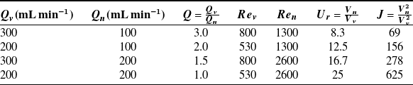
 Q=QvQn
 20∘
20∘ 40∘
40∘ 60∘
60∘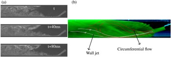
 Q=3
Q=3
 Q=3
Q=3 x/d
x/d
 Q=2
Q=2 Q=1.5
Q=1.5 Q=1
Q=1
 Q=3
Q=3 U
U U
U x/d
x/d U0
U0 U0
U0 U
U
 U
U Q
Q Q
Q Q
Q
 (x,z)
(x,z) U
U Q
Q
 Q=3
Q=3 ∘
∘ ∘
∘ ∘
∘
 x/d=25
 U
U x/d=25
 Q
Q
 Q=3
Q=3 ∘
∘
 Q
Q


 Open access

