





Impact statement
This study introduces a consistent hierarchical Bayesian method for time-varying finite element model updating, enabling more accurate and reliable structural health monitoring under environmental variability. Formulated in a coherent Bayesian framework, the method provides more reliable and realistic parameter estimates than traditional approaches. It avoids the need for tedious modal matching and handles incomplete modal data, making it practical for real-world applications. The proposed sampling strategy ensures computational efficiency and robustness. This work supports better decision-making in structural maintenance and enhances the sustainability of infrastructure systems.
1. Introduction
The finite element (FE) method is a widely used numerical analysis tool to simulate the structural response under various load conditions. Despite its extensive use, practical challenges, such as uncertainties in environmental conditions, material properties, boundary conditions, and load scenarios, often prevent theoretical models from accurately reflecting actual conditions (He et al., Reference He, Reynders, Garcia-Palacios, Marano, Briseghella and De Roeck2020; Sun et al., Reference Sun, Li and Zhang2020). To address this issue, the finite element model updating (FEMU) is commonly used to adjust various parameters in the FE model according to the measured data, ensuring that the calculated responses match the measured data to the greatest extent. By comparing the changes in model parameters, it is possible to infer the existence, location, and severity of potential damage in the structure (Mottershead and Friswell, Reference Mottershead and Friswell1993; Carden and Fanning, Reference Carden and Fanning2004; Friswell, Reference Friswell2007). Therefore, it is of critical importance to align the FE model with measured data.
Sensitivity-based FEMU is one of the most widely used approaches, aimed at identifying the structural parameters by minimizing the difference between the model outputs and the observed data. It takes advantage of the sensitivity of parameters to iteratively update the model (Ereiz et al., Reference Ereiz, Duvnjak and Jimenez-Alonso2022). Jaishi and Ren (Reference Jaishi and Ren2005) formulated a least-squares method to minimize the objective function composed of frequency residuals, modal-shape-related functions, and modal flexibility residuals. Razavi and Hadidi (Reference Razavi and Hadidi2020) investigated the robustness of sensitivity-based model updating for damage detection of large structures by minimizing the discrepancy in acceleration responses. Cao et al. (Reference Cao, Wei, Liang, Jia, Yao and Jiang2023) established a non-intrusive dynamic sensitivity-based FEMU method using an enhanced Hurty/Craig–Bampton approach for nonlinear substructures. Although demonstrating strong adaptability, the sensitivity-based FEMU method often gets trapped in local minima (Teughels and De Roeck, Reference Teughels and De Roeck2004) and is highly dependent on selecting proper initial values.
Global optimization methods, such as the particle swarm optimization (PSO) (Pham et al., Reference Pham, D-K and Kim2024), efficient global optimization (EGO) (Yang et al., Reference Yang, Guo, Ouyang and Li2017), simulated annealing, and genetic algorithm (Standoli et al., Reference Standoli, Salachoris, Masciotta and Clementi2021), are other commonly used approaches. These methods have also found extensive application in the realm of FEMU, and their capabilities and limitations have been thoroughly examined. For instance, Yang et al. (Reference Yang, Guo, Ouyang and Li2017) developed a model updating method using a surrogate Kriging model to construct the nonlinear response surface of the objective function and employed an EGO algorithm for producing results. Girardi et al. (Reference Girardi, Padovani, Pellegrini and Robol2021) introduced a multi-start global optimization approach using local parametric reduced-order models to address constrained minimization problems in FEMU. Pham et al. (Reference Pham, D-K and Kim2024) proposed a PSO and the categorical gradient boosting algorithm to identify cable damage in cable-stayed bridges. Although these optimization algorithms possess solid theoretical foundations, they often encounter challenges related to low computational efficiency in practice, particularly when dealing with large-scale data or complex problems.
These methods typically rely on accurate measurement data and clear physical parameters, yet errors often arise from imperfect measurement, random noise, signal processing issues, and challenges in data post-processing (Dhandole and Modak, Reference Dhandole and Modak2012). Additionally, structural parameters, along with boundary and continuity conditions, are subject to change over time due to environmental influences and varying operating conditions, leading to time-varying parameters in the model. To ensure reliable damage diagnosis and prognosis, it is essential to explicitly account for these time variations in FEMU. For example, Li et al. (Reference Li, Zhou and He2025b) developed a state estimation framework to address the time-varying system identification problem. Since it aims at real-time parameter tracking, the computation is usually demanding, especially when dealing with complicated and high-dimensional FE models.
For a robust FEMU, Bayesian inference has been adopted for FEMU by incorporating parametric uncertainty, modeling error, and measurement error (Adeagbo et al., Reference Adeagbo, Liu, Yang, Huang and Lam2025). Beck and his colleagues have played a key role in the early development of Bayesian methods for FEMU (Beck and Katafygiotis, Reference Beck and Katafygiotis1998; Vanik and Beck, Reference Vanik and Beck1998; Papadimitriou et al., Reference Papadimitriou, Beck and Katafygiotis2001; Beck and Au, Reference Beck and Au2002; Yang and Lam, Reference Yang and Lam2018). To improve the efficiency of Bayesian updating, recent studies have focused on developing advanced sampling strategies. For instance, Meng et al. (Reference Meng, Beck, Huang and Li2025) first proposed an innovative Adaptive Meta-learning SGHMC algorithm for Bayesian updating of complex posterior distributions. By incorporating retraining-free, scale-invariant neural networks, this approach significantly enhances both the efficiency and generalization capability of MCMC simulations. However, applying Bayesian inference to high-dimensional FE models is computationally demanding, particularly for real-time or large-scale problems. To address this, alternative strategies such as surrogate-based methods (Sengupta and Chakraborty, Reference Sengupta and Chakraborty2025) and likelihood-free approaches (Beaumont, Reference Beaumont and Reid2019) have been explored. Surrogate models improve computational efficiency by approximating the forward model but may introduce errors, while likelihood-free methods avoid explicit likelihood formulation at the cost of potential subjectivity. Despite these advancements, many traditional approaches fail to account for the intrinsic variability introduced by environmental factors, resulting in an underestimation of parameter uncertainty.
The hierarchical Bayes approach has been applied to capture the variability of structural parameters (Behmanesh et al., Reference Behmanesh, Moaveni, Lombaert and Papadimitriou2015; Xue et al., Reference Xue, Zhou, Beck, Huang and Li2023). However, a common issue with previous algorithms is the need for modal order matching and the ignorance of the statistical correlation between parameters. In addition, many earlier Bayesian FEMU approaches adopted an inappropriate likelihood function, such as unclear error distribution assumptions (Ching et al., Reference Ching, Muto and Beck2006) and incorrect normalization factors (Yuen et al., Reference Yuen, Beck and Katafygiotis2006; Yan and Katafygiotis, Reference Yan and Katafygiotis2015), resulting in biased parameter estimation. Recent studies have introduced improvements to address the above issues. For instance, Huang et al. (Reference Huang, Beck and Li2017) transformed the eigenvalue equation into a probabilistic constraint, incorporating random errors, and incorporated it into the joint prior distribution of system modal parameters and stiffness parameters, thereby avoiding modal matching. Luo et al. (Reference Luo, Song, Li and Sun2025) utilized a response surface model to directly map parameters to responses, introduced hyperparameters and covariance matrices for temperature and vehicle loads, and explicitly modeled systematic bias and random errors.
Building on these previous works, this paper proposes an improved three-layer hierarchical Bayesian framework to capture the time-varying stiffness parameters, caused by environmental variability, for example, temperature and humidity. Specifically, a time-invariant hyperparameter is introduced at the upper level to regulate the evolution of time-varying stiffness parameters, while appropriate priors and covariance structures are assigned to enhance robustness and uncertainty quantification. The proposed framework adopts a fully probabilistic formulation with an explicitly derived likelihood grounded in the physical model. This endows the method with a solid theoretical foundation, characterized by a rigorously derived likelihood and strong adherence to physical principles.
A key methodological advance of the proposed framework lies in the probabilistic treatment of mode shapes. Instead of treating measured or expanded mode shapes as deterministic quantities obtained through preprocessing, the unmeasured mode shapes are explicitly modeled as latent random variables within the Bayesian hierarchy. This latent-variable formulation enables the joint inference of structural parameters and modal quantities in a fully generative manner, thereby eliminating the need for modal matching and explicit eigenvalue decomposition. Furthermore, the geometric nature of mode shapes is rigorously respected by constraining them to the unit hypersphere using a Bingham distribution, which ensures statistical consistency and physically meaningful uncertainty representation. Compared with conventional plug-in or two-stage approaches, this strategy provides improved robustness and avoids biases introduced by deterministic modal expansion.
The outline of the paper is as follows. First, the FEMU problem is reformulated within a probabilistic framework by modeling uncertainties in both measurements and modeling errors. Next, a hierarchical Bayesian formulation with latent mode shapes is developed for joint parameter inference. A Metropolis-within-Gibbs (MwG) sampler is developed to approximate the posterior, together with a robust implementation strategy. Finally, three empirical studies, including synthetic data, laboratory experiments, and field tests, are presented to demonstrate the effectiveness and performance of the proposed algorithm.
2. Problem formulation
The problem of FEMU considered here is to find a good FE model to numerically represent the true structure, given the measured modal frequencies
$ {\omega}_{kt}\in {\mathbb{R}}^{+} $
 and mode shapes
$ {\boldsymbol{\phi}}_{kt}^m\in {\mathbb{R}}^{N_o} $
and mode shapes
$ {\boldsymbol{\phi}}_{kt}^m\in {\mathbb{R}}^{N_o} $
 , for
$ k=1,2,\dots, {N}_m $
, for
$ k=1,2,\dots, {N}_m $
 and
$ t=1,2,\dots, T $
and
$ t=1,2,\dots, T $
 , in which
$ {N}_o $
, in which
$ {N}_o $
 is the number of measured degrees of freedom (DoFs) over the structure,
$ {N}_m $
is the number of measured degrees of freedom (DoFs) over the structure,
$ {N}_m $
 is the number of measured modes, and
$ T $
is the number of measured modes, and
$ T $
 is the total number of available datasets. The superscript
$ m $
is the total number of available datasets. The superscript
$ m $
 on
$ {\boldsymbol{\phi}}_{kt}^m $
on
$ {\boldsymbol{\phi}}_{kt}^m $
 indicates that only the measured DoFs are represented in this mode shape vector. Since in Bayesian data analysis a true fixed value is assumed for each parameter (Gelman et al., Reference Gelman, Carlin, Stern, Dunson, Vehtari and Rubin2013), the posterior distribution of the parameters will underestimate the inherent uncertainty with more and more data collected, if the time-dependent behavior (represented by the symbol
$ t $
indicates that only the measured DoFs are represented in this mode shape vector. Since in Bayesian data analysis a true fixed value is assumed for each parameter (Gelman et al., Reference Gelman, Carlin, Stern, Dunson, Vehtari and Rubin2013), the posterior distribution of the parameters will underestimate the inherent uncertainty with more and more data collected, if the time-dependent behavior (represented by the symbol
$ t $
 here) is ignored.
The basic assumptions on the structural model are that it is linear and classically damped, but it can be time-variant. Given the assumption of classical damping, only modal frequencies and mode shapes are necessary in order to identify the mass matrix
$ \boldsymbol{M}\in {\mathbb{R}}^{N_d\times {N}_d} $
 and stiffness matrix
$ \boldsymbol{K}\in {\mathbb{R}}^{N_d\times {N}_d} $
and stiffness matrix
$ \boldsymbol{K}\in {\mathbb{R}}^{N_d\times {N}_d} $
 , where
$ {N}_d $
, where
$ {N}_d $
 is the number of DoFs of the FE model. In this paper, we assume that we know the mass matrix
$ \boldsymbol{M}\in {\mathbb{R}}^{N_d\times {N}_d} $
is the number of DoFs of the FE model. In this paper, we assume that we know the mass matrix
$ \boldsymbol{M}\in {\mathbb{R}}^{N_d\times {N}_d} $
 , because it usually can be established with sufficient accuracy from the engineering drawings of the structure. The stiffness matrix
$ \boldsymbol{K}\in {\mathbb{R}}^{N_d\times {N}_d} $
, because it usually can be established with sufficient accuracy from the engineering drawings of the structure. The stiffness matrix
$ \boldsymbol{K}\in {\mathbb{R}}^{N_d\times {N}_d} $
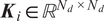
 is modeled in an affine manner, that is, as the weighted sum of a nominal stiffness matrix
$ {\boldsymbol{K}}_0\in {\mathbb{R}}^{N_d\times {N}_d} $
is modeled in an affine manner, that is, as the weighted sum of a nominal stiffness matrix
$ {\boldsymbol{K}}_0\in {\mathbb{R}}^{N_d\times {N}_d} $
 and a series of substructure stiffness matrices
$ {\boldsymbol{K}}_i\in {\mathbb{R}}^{N_d\times {N}_d} $
and a series of substructure stiffness matrices
$ {\boldsymbol{K}}_i\in {\mathbb{R}}^{N_d\times {N}_d} $
 for
$ i=1,2,\dots, {N}_k $
for
$ i=1,2,\dots, {N}_k $
 as
as

in which
$ {\boldsymbol{\kappa}}_t={\left[{\kappa}_{1t},{\kappa}_{2t},\dots, {\kappa}_{N_kt}\right]}^{\mathrm{T}} $
 is a set of dimensionless parameters describing possible modifications of the nominal stiffness in time. Note that under the assumption of linear structural behavior, we can always write the stiffness matrix in the form of Equation (2.1) by modeling
$ {\boldsymbol{K}}_i $
is a set of dimensionless parameters describing possible modifications of the nominal stiffness in time. Note that under the assumption of linear structural behavior, we can always write the stiffness matrix in the form of Equation (2.1) by modeling
$ {\boldsymbol{K}}_i $
 as a subset of element stiffness matrices. This representation of the stiffness matrix has been used in previous works (Ching and Chen, Reference Ching and Chen2007; Ching et al., Reference Ching, Muto and Beck2006; Ching and Beck, Reference Ching and Beck2004; Vanik and Beck, Reference Vanik and Beck1998).
2.1. Physical model
The relation between the unknown parameters
$ {\boldsymbol{\kappa}}_t $
 and the measured modal parameters
$ {\omega}_{kt} $
and the measured modal parameters
$ {\omega}_{kt} $
 and
$ {\boldsymbol{\phi}}_{kt}^m $
and
$ {\boldsymbol{\phi}}_{kt}^m $
 can generally be given by the following two equations:


where
$ \boldsymbol{H}\left({\boldsymbol{\kappa}}_t,{\lambda}_{kt}\right)=\boldsymbol{K}\left({\boldsymbol{\kappa}}_t\right)-{\lambda}_{kt}\boldsymbol{M} $
 denotes a linear matrix pencil,
$ \det \left[\bullet \right] $
denotes a linear matrix pencil,
$ \det \left[\bullet \right] $
 is the matrix determinant and
$ {\lambda}_{kt}={\omega}_{kt}^2 $
is the matrix determinant and
$ {\lambda}_{kt}={\omega}_{kt}^2 $
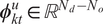
 represents the generalized eigenvalue. The generalized eigenvector consists of measured and unmeasured mode shapes
$ {\boldsymbol{\phi}}_{kt}^m $
represents the generalized eigenvalue. The generalized eigenvector consists of measured and unmeasured mode shapes
$ {\boldsymbol{\phi}}_{kt}^m $
 and
$ {\boldsymbol{\phi}}_{kt}^u\in {\mathbb{R}}^{N_d-{N}_o} $
and
$ {\boldsymbol{\phi}}_{kt}^u\in {\mathbb{R}}^{N_d-{N}_o} $
 , that is,
$ {\boldsymbol{\phi}}_{kt}={\boldsymbol{P}}_{\phi }{\left[{{\boldsymbol{\phi}}_{kt}^m}^{\mathrm{T}}\;{{\boldsymbol{\phi}}_{kt}^u}^{\mathrm{T}}\right]}^{\mathrm{T}} $
, that is,
$ {\boldsymbol{\phi}}_{kt}={\boldsymbol{P}}_{\phi }{\left[{{\boldsymbol{\phi}}_{kt}^m}^{\mathrm{T}}\;{{\boldsymbol{\phi}}_{kt}^u}^{\mathrm{T}}\right]}^{\mathrm{T}} $
 . The above two equations represent the most fundamental ones. Other equations, such as the orthogonality condition of mode shapes, can be derived consequently. Note that Equations (2.2) and (2.3) are not redundant; in particular, Equation (2.2) can be used to estimate the eigenvalue
$ {\lambda}_{kt} $
. The above two equations represent the most fundamental ones. Other equations, such as the orthogonality condition of mode shapes, can be derived consequently. Note that Equations (2.2) and (2.3) are not redundant; in particular, Equation (2.2) can be used to estimate the eigenvalue
$ {\lambda}_{kt} $
 without knowing the eigenvector
$ {\boldsymbol{\phi}}_{kt} $
without knowing the eigenvector
$ {\boldsymbol{\phi}}_{kt} $
 , but Equation (2.3) is needed to estimate the eigenvectors.
A key drawback of directly applying Equation (2.2) is the potentially large numerical error in computing the determinant of
$ \boldsymbol{H}\left({\boldsymbol{\kappa}}_t,{\lambda}_{kt}\right) $
 , especially when the number of DoFs
$ {N}_d $
, especially when the number of DoFs
$ {N}_d $
 is large. Since the determinant equals the product of all eigenvalues, its magnitude can grow exponentially with increasing
$ {N}_d $
is large. Since the determinant equals the product of all eigenvalues, its magnitude can grow exponentially with increasing
$ {N}_d $
 , leading to numerical instability. For numerical stability, we adopt an equivalent formulation based on the minimum singular value. That is, if
$ {\lambda}_{kt} $
, leading to numerical instability. For numerical stability, we adopt an equivalent formulation based on the minimum singular value. That is, if
$ {\lambda}_{kt} $
 is a generalized eigenvalue of the pair
$ \left[\boldsymbol{K}\left({\boldsymbol{\kappa}}_t\right),\boldsymbol{M}\right] $
is a generalized eigenvalue of the pair
$ \left[\boldsymbol{K}\left({\boldsymbol{\kappa}}_t\right),\boldsymbol{M}\right] $
 , then the matrix
$ \boldsymbol{H}\left({\boldsymbol{\kappa}}_t,{\lambda}_{kt}\right) $
, then the matrix
$ \boldsymbol{H}\left({\boldsymbol{\kappa}}_t,{\lambda}_{kt}\right) $
 becomes singular, yielding a zero minimum singular value. As a result, we transform Equation (2.2) into

in which
$ {\sigma}_{\mathrm{min}}\left[\bullet \right] $
 denotes the minimum singular value. This approach requires only the evaluation of the minimum singular value, bypassing the unstable computation of the determinant.
Equations (2.3) and (2.4) provide the deterministic relation between the unknown parameters
$ {\boldsymbol{\kappa}}_t $
 and the measured modal parameters
$ {\omega}_{kt} $
and the measured modal parameters
$ {\omega}_{kt} $
 and
$ {\boldsymbol{\phi}}_{kt}^m $
and
$ {\boldsymbol{\phi}}_{kt}^m $
 . However, due to the existence of uncertainties, these equations cannot be strictly satisfied. On the one hand,
$ \boldsymbol{K}\left({\boldsymbol{\kappa}}_t\right) $
. However, due to the existence of uncertainties, these equations cannot be strictly satisfied. On the one hand,
$ \boldsymbol{K}\left({\boldsymbol{\kappa}}_t\right) $
 is only an idealization of the complex structure with simplifications, so that there are always modeling errors in
$ \boldsymbol{K}\left({\boldsymbol{\kappa}}_t\right) $
is only an idealization of the complex structure with simplifications, so that there are always modeling errors in
$ \boldsymbol{K}\left({\boldsymbol{\kappa}}_t\right) $
 . On the other hand,
$ {\omega}_{kt} $
. On the other hand,
$ {\omega}_{kt} $
 and
$ {\boldsymbol{\phi}}_{kt}^m $
and
$ {\boldsymbol{\phi}}_{kt}^m $
 cannot be measured exactly as measurement errors are inevitable. Considering these errors, we have the following stochastic equations:


where
$ {w}_{kt} $
 and
$ {\boldsymbol{v}}_{kt} $
and
$ {\boldsymbol{v}}_{kt} $
 represent the combined effects of the modeling error and the measurement error.
Here, we model the true structure by a time-varying FE model because of the changing environmental effects and operational conditions. Assuming the existence of a fixed model for a reference environment and operational conditions, we have the following linear equation:

in which
$ \boldsymbol{\kappa} $
 is a deterministic unknown set of parameters of the true reference model and
$ {\boldsymbol{\varepsilon}}_t $
is a deterministic unknown set of parameters of the true reference model and
$ {\boldsymbol{\varepsilon}}_t $
 models the time-varying environmental and other effects, which are not explicitly measured.
2.2. Probabilistic model
The difficulty in constructing the probabilistic model for FEMU lies in the formulation of the conditional probability distributions of
$ {\lambda}_{kt} $
 and
$ {\boldsymbol{\phi}}_{kt}^m $
and
$ {\boldsymbol{\phi}}_{kt}^m $
 , given
$ {\boldsymbol{\kappa}}_t $
, given
$ {\boldsymbol{\kappa}}_t $
 , that is, the likelihood function. In this section, we propose a probabilistic model for FEMU based on the physical model introduced in the last section by assigning probability distributions to the noise terms
$ {w}_{kt} $
, that is, the likelihood function. In this section, we propose a probabilistic model for FEMU based on the physical model introduced in the last section by assigning probability distributions to the noise terms
$ {w}_{kt} $
 ,
$ {\boldsymbol{v}}_{kt} $
,
$ {\boldsymbol{v}}_{kt} $
 and
$ {\boldsymbol{\varepsilon}}_t $
and
$ {\boldsymbol{\varepsilon}}_t $
 and by specifying prior distributions for the unknown parameters
$ {\boldsymbol{\kappa}}_t $
and by specifying prior distributions for the unknown parameters
$ {\boldsymbol{\kappa}}_t $
 .
.
Following the principle of maximum entropy (Jaynes, Reference Jaynes1957), we assume that
$ {w}_{kt} $
 and
$ {\boldsymbol{v}}_{kt} $
and
$ {\boldsymbol{v}}_{kt} $
 both follow normal distributions, and they are independent of each other, that is, with the following PDFs
$ f\left({w}_{kt}|{\alpha}_k\right)=\mathrm{N}\left(0,{\alpha}_k^{-1}{\left\Vert {\overline{\lambda}}_k\boldsymbol{M}\right\Vert}_2^2\right) $
both follow normal distributions, and they are independent of each other, that is, with the following PDFs
$ f\left({w}_{kt}|{\alpha}_k\right)=\mathrm{N}\left(0,{\alpha}_k^{-1}{\left\Vert {\overline{\lambda}}_k\boldsymbol{M}\right\Vert}_2^2\right) $
 and
$ f\left({\boldsymbol{v}}_{kt}|{\beta}_k\right)=\mathrm{N}\left(\mathbf{0},{\beta}_k^{-1}{\left\Vert {\overline{\lambda}}_k\boldsymbol{M}\right\Vert}_2^2\boldsymbol{I}\right) $
and
$ f\left({\boldsymbol{v}}_{kt}|{\beta}_k\right)=\mathrm{N}\left(\mathbf{0},{\beta}_k^{-1}{\left\Vert {\overline{\lambda}}_k\boldsymbol{M}\right\Vert}_2^2\boldsymbol{I}\right) $
 . Here,
$ {\left\Vert \bullet \right\Vert}_2 $
. Here,
$ {\left\Vert \bullet \right\Vert}_2 $
 denotes the L2-norm of a matrix,
$ {\overline{\lambda}}_k $
denotes the L2-norm of a matrix,
$ {\overline{\lambda}}_k $
 is the median of eigenvalues of
$ {\boldsymbol{K}}_0/{\left\Vert \boldsymbol{M}\right\Vert}_2 $
is the median of eigenvalues of
$ {\boldsymbol{K}}_0/{\left\Vert \boldsymbol{M}\right\Vert}_2 $
 , and
$ \boldsymbol{I} $
, and
$ \boldsymbol{I} $
 represent an identity matrix of proper size. Here, we define the variance/covariance matrix to depend on the scale of the system. This is realistic from an engineering perspective because varying scales of structures generally yield different levels of residuals in Equations (2.5) and (2.6). Therefore, the precision parameters
$ {\alpha}_k $
represent an identity matrix of proper size. Here, we define the variance/covariance matrix to depend on the scale of the system. This is realistic from an engineering perspective because varying scales of structures generally yield different levels of residuals in Equations (2.5) and (2.6). Therefore, the precision parameters
$ {\alpha}_k $
 and
$ {\beta}_k $
and
$ {\beta}_k $
 become dimensionless, facilitating the inference from data. More benefits will be discussed in the posterior inference in Section 3.1.
This choice of variance/covariance is effectively a way of implementing a Jeffreys prior (Gelman et al., Reference Gelman, Carlin, Stern, Dunson, Vehtari and Rubin2013) for scale parameters. In Bayesian statistics, when we do not know the scale of a variable, an objective choice of a prior should be invariant to changes in units. By scaling the variance/covariance by
$ {\left\Vert {\overline{\lambda}}_k\boldsymbol{M}\right\Vert}_2^2 $
 , it is essentially forcing the model to ignore the absolute magnitude of the mass/stiffness. This is a non-informative and objective way to set up the problem, ensuring that the data (the measured modal frequencies and mode shapes) drives the results, rather than the mathematical artifacts of the normal distribution.
The independence assumption between
$ {w}_{kt} $
 and
$ {\boldsymbol{v}}_{kt} $
and
$ {\boldsymbol{v}}_{kt} $
 is mainly for mathematical convenience, and as we will see later, this will not remove the targeted correlation within
$ {\boldsymbol{\kappa}}_t $
is mainly for mathematical convenience, and as we will see later, this will not remove the targeted correlation within
$ {\boldsymbol{\kappa}}_t $
 and
$ \boldsymbol{\kappa} $
and
$ \boldsymbol{\kappa} $
 . In addition, independence is assumed for
$ {w}_{kt} $
. In addition, independence is assumed for
$ {w}_{kt} $
 and
$ {\boldsymbol{v}}_{kt} $
and
$ {\boldsymbol{v}}_{kt} $
 for different modes and different time instances. The time independence is generally valid because the modal identification in structural health monitoring usually involves a long period of data, so that the time correlation becomes negligible. The modal independence is validated by the recently developed uncertainty laws in modal identification (Au et al., Reference Au, Brownjohn, Li and Raby2021), stating that correlation exists only for very closely spaced modes. Since most structural modes are well-separated, we will adopt the modal independence assumption to simplify the formulation.
To derive the distribution of the generalized eigenvalue
$ {\lambda}_{kt} $
 , we apply the rule of change-of-variables from the error distribution of
$ {w}_{kt} $
, we apply the rule of change-of-variables from the error distribution of
$ {w}_{kt} $
 (Ching et al., Reference Ching, Muto and Beck2006) to obtain

where
$ {\boldsymbol{\psi}}_{\mathrm{min}} $
 is the singular vector that corresponds to the minimum singular value of
$ \boldsymbol{H}\left({\boldsymbol{\kappa}}_t,{\lambda}_{kt}\right) $
is the singular vector that corresponds to the minimum singular value of
$ \boldsymbol{H}\left({\boldsymbol{\kappa}}_t,{\lambda}_{kt}\right) $
 . Note that, in the case of a small error
$ {\boldsymbol{v}}_{kt}\to 0 $
. Note that, in the case of a small error
$ {\boldsymbol{v}}_{kt}\to 0 $
 ,
$ {\boldsymbol{\psi}}_{\mathrm{min}}\to {\boldsymbol{\phi}}_{kt} $
,
$ {\boldsymbol{\psi}}_{\mathrm{min}}\to {\boldsymbol{\phi}}_{kt} $
 and
$ {\boldsymbol{\psi}}_{\mathrm{min}}^{\mathrm{T}}\boldsymbol{M}{\boldsymbol{\psi}}_{\mathrm{min}} $
and
$ {\boldsymbol{\psi}}_{\mathrm{min}}^{\mathrm{T}}\boldsymbol{M}{\boldsymbol{\psi}}_{\mathrm{min}} $
 converges to the
$ k $
converges to the
$ k $
 -th modal mass.
For mode shapes, special care is required due to their intrinsic geometric constraints. Mode shapes are defined only up to scale and sign (i.e.,
$ {\boldsymbol{\phi}}_{kt} $
 and
$ -c{\boldsymbol{\phi}}_{kt} $
and
$ -c{\boldsymbol{\phi}}_{kt} $
 represent the same mode shape, where
$ c $
represent the same mode shape, where
$ c $
 represents an arbitrary constant), and their physically meaningful representation lies on a constrained manifold of the unit hypersphere. Rather than treating mode shapes as unconstrained Euclidean random vectors and introducing Jacobian correction terms via change-of-variable arguments, we define the probability measure directly on the appropriate Riemannian manifold. This approach ensures that probability mass is distributed consistently with the underlying geometry of the mode shape space.
Uncertainty in the mode shapes is induced through the eigen-equation residual
$ {\boldsymbol{v}}_{kt} $
 . With the scale-invariant error model of
$ {\boldsymbol{v}}_{kt} $
. With the scale-invariant error model of
$ {\boldsymbol{v}}_{kt} $
 , the likelihood of the normalized mode shape
$ {\boldsymbol{\phi}}_{kt} $
, the likelihood of the normalized mode shape
$ {\boldsymbol{\phi}}_{kt} $
 depends on the quadratic form
$ {\boldsymbol{\phi}}_{kt}^{\mathrm{T}}\boldsymbol{H}{\left({\boldsymbol{\kappa}}_t,{\lambda}_{kt}\right)}^{\mathrm{T}}\boldsymbol{H}\left({\boldsymbol{\kappa}}_t,{\lambda}_{kt}\right){\boldsymbol{\phi}}_{kt} $
depends on the quadratic form
$ {\boldsymbol{\phi}}_{kt}^{\mathrm{T}}\boldsymbol{H}{\left({\boldsymbol{\kappa}}_t,{\lambda}_{kt}\right)}^{\mathrm{T}}\boldsymbol{H}\left({\boldsymbol{\kappa}}_t,{\lambda}_{kt}\right){\boldsymbol{\phi}}_{kt} $
 . With the unit-norm constraint imposed (
$ {\boldsymbol{\phi}}_{kt}^{\mathrm{T}}{\boldsymbol{\phi}}_{kt}=1 $
. With the unit-norm constraint imposed (
$ {\boldsymbol{\phi}}_{kt}^{\mathrm{T}}{\boldsymbol{\phi}}_{kt}=1 $
 ), the resulting probability density on the unit hypersphere (with respect to the Riemannian measure) is a Bingham distribution (Kent, Reference Kent1982).

This distribution is invariant to sign changes of the mode shape and naturally concentrates around directions that best satisfy the eigen-equation. The normalizing constant
$ {z}_{kt}\left({\boldsymbol{\kappa}}_t,{\lambda}_{kt}\right) $
 is the integral of the exponential term over the sphere. In structural systems,
$ \boldsymbol{H}\left({\boldsymbol{\kappa}}_t,{\lambda}_{kt}\right) $
is the integral of the exponential term over the sphere. In structural systems,
$ \boldsymbol{H}\left({\boldsymbol{\kappa}}_t,{\lambda}_{kt}\right) $
 possesses one singular (or near-singular) eigenvalue associated with the modal direction and
$ {N}_d-1 $
possesses one singular (or near-singular) eigenvalue associated with the modal direction and
$ {N}_d-1 $
 significantly larger eigenvalues in the orthogonal directions. In this high-concentration setting, the normalizing constant can be accurately approximated by (Mardia and Jupp, Reference Mardia and Jupp1999):

where
$ {\det}^{\ast}\left[\bullet \right] $
 denotes the pseudo-determinant (the product of the
$ {N}_d-1 $
denotes the pseudo-determinant (the product of the
$ {N}_d-1 $
 eigenvalues significantly greater than zero). This term serves as a geometric curvature correction, replacing the vanishing Jacobian factors that cause singularities in unconstrained change-of-variable derivations.
Since the above PDF is not standard, it is interesting to see its shape through a simple example. Suppose we have a model with the following parameters:

This two-degree-of-freedom system has two distinct modes, and here we focus on the second mode with an eigenvalue of
$ {\lambda}_2=3.41 $
 . Considering
$ \kappa =0 $
. Considering
$ \kappa =0 $
 and
$ {\alpha}_k=200 $
and
$ {\alpha}_k=200 $
 , the PDF in Equation (2.8) is plotted in Figure 1. It can be inferred that this distribution centers around the eigenvalue of the deterministic model. For the simple example in Equation (2.11), the PDF of the second mode shape for selected
$ \kappa $
, the PDF in Equation (2.8) is plotted in Figure 1. It can be inferred that this distribution centers around the eigenvalue of the deterministic model. For the simple example in Equation (2.11), the PDF of the second mode shape for selected
$ \kappa $
 values is illustrated in Figure 2, where we have set
$ {\beta}_k=100 $
values is illustrated in Figure 2, where we have set
$ {\beta}_k=100 $
 . As the value of
$ \kappa $
. As the value of
$ \kappa $
 approaches the true value
$ 0 $
approaches the true value
$ 0 $
 , the PDF becomes increasingly concentrated toward the true value corresponding to
$ \kappa =0 $
, the PDF becomes increasingly concentrated toward the true value corresponding to
$ \kappa =0 $
 .
.
Derived distributions of eigenvalue.

Derived distributions of eigenvector for different values of κ: (a) κ = 1.0, (b) κ = 0.5, and (c) κ = 0.05. Note: black arrows show the mean direction of each Bingham distribution, while red arrows indicate the mean direction when
$ \unicode{x03BA} =0 $
 .
.
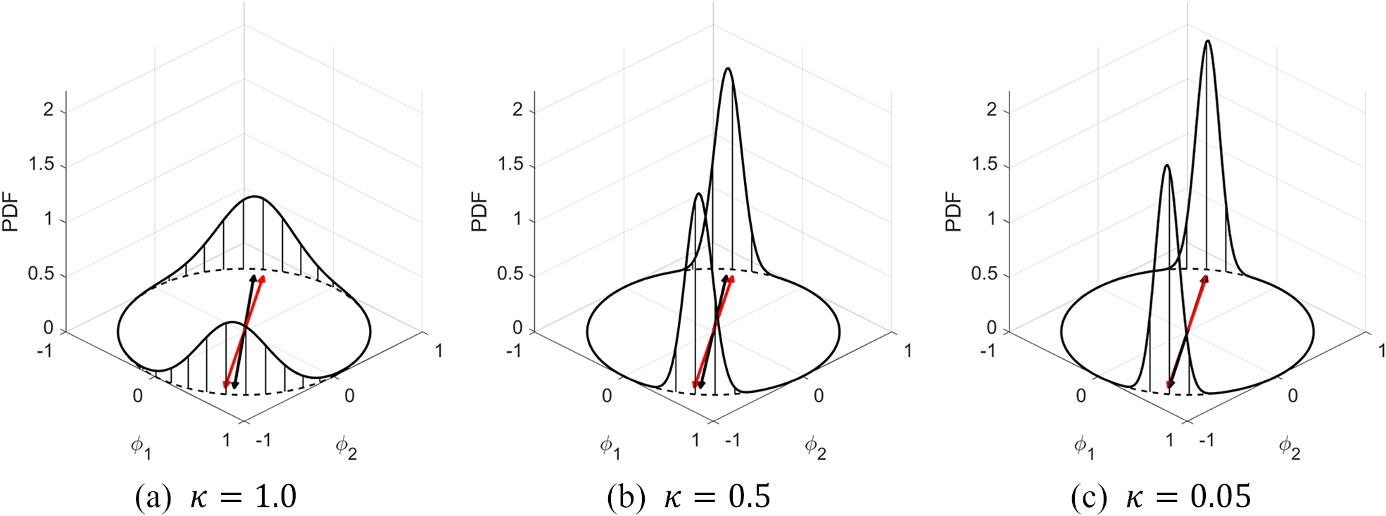
Figure 2. Long description
From left to right, each panel presents a 3D probability density function surface plotted over phi one (horizontal axis) and phi two (depth axis), with P D F on the vertical axis. Panel a, labeled kappa equals 1.0, shows a broad, rounded surface with a black arrow pointing upward and slightly right from the origin, and a red arrow diverging at a smaller angle. Panel b, labeled kappa equals 0.5, displays a narrower, taller surface with both black and red arrows closer together and more vertical. Panel c, labeled kappa equals 0.05, features a sharply peaked surface with both arrows nearly overlapping and pointing steeply upward. The black arrow in each panel marks the mean direction of the Bingham distribution, while the red arrow marks the mean direction for kappa equals zero. The base of each surface is a circular contour of radius 1 in the phi one–phi two plane.
In addition, by assuming
$ {\boldsymbol{\varepsilon}}_t $
 to be a zero-mean multivariate normal random vector with a precision matrix
$ \boldsymbol{P} $
to be a zero-mean multivariate normal random vector with a precision matrix
$ \boldsymbol{P} $
 , according to Equation (2.7), we have the conditional distribution of
$ {\boldsymbol{\kappa}}_t $
, according to Equation (2.7), we have the conditional distribution of
$ {\boldsymbol{\kappa}}_t $
 given
$ \boldsymbol{\kappa} $
given
$ \boldsymbol{\kappa} $
 and
$ \boldsymbol{P} $
and
$ \boldsymbol{P} $
 as
as

As for the prior distributions for the parameters
$ \boldsymbol{\theta} =\left\{\boldsymbol{\kappa}, \boldsymbol{P},\boldsymbol{\alpha}, \boldsymbol{\beta} \right\} $
 , the following conjugate prior distributions are assigned (Gelman et al., Reference Gelman, Carlin, Stern, Dunson, Vehtari and Rubin2013).


where
$ {\boldsymbol{E}}_0 $
 is a scale matrix, and
$ {e}_0 $
is a scale matrix, and
$ {e}_0 $
 represents the DoFs for the Wishart distribution;
$ {p}_0 $
represents the DoFs for the Wishart distribution;
$ {p}_0 $
 is a scale factor, and
$ {\boldsymbol{\kappa}}_0 $
is a scale factor, and
$ {\boldsymbol{\kappa}}_0 $
 reflect the prior belief about
$ \boldsymbol{\kappa} $
reflect the prior belief about
$ \boldsymbol{\kappa} $
 in the absence of data;
$ {u}_{k,0} $
in the absence of data;
$ {u}_{k,0} $
 and
$ {r}_{k,0} $
and
$ {r}_{k,0} $
 are the shape parameters for the PDF of random variables
$ {\alpha}_k $
are the shape parameters for the PDF of random variables
$ {\alpha}_k $
 and
$ {\beta}_k $
and
$ {\beta}_k $
 , respectively, while
$ {h}_{k,0} $
, respectively, while
$ {h}_{k,0} $
 and
$ {s}_{k,0} $
and
$ {s}_{k,0} $
 are the corresponding scale parameters.
It should be noted that
$ \pi \left(\boldsymbol{P}\right) $
 and
$ \pi \left(\boldsymbol{\kappa} |\boldsymbol{P}\right) $
and
$ \pi \left(\boldsymbol{\kappa} |\boldsymbol{P}\right) $
 are hyperpriors, while
$ \pi \left(\boldsymbol{\alpha} \right) $
are hyperpriors, while
$ \pi \left(\boldsymbol{\alpha} \right) $
 ,
$ \pi \left(\boldsymbol{\beta} \right) $
,
$ \pi \left(\boldsymbol{\beta} \right) $
 and
$ f\left({\boldsymbol{\kappa}}_t|\boldsymbol{\kappa}, \boldsymbol{P}\right) $
and
$ f\left({\boldsymbol{\kappa}}_t|\boldsymbol{\kappa}, \boldsymbol{P}\right) $
 are priors. Combining Equations (2.8) and (2.14)–(2.16) yields the joint distribution of the observed variables
$ \boldsymbol{y}=\left\{{\lambda}_{kt},{\boldsymbol{\phi}}_{kt}^m,k=1:{N}_m,t=1:T\right\} $
are priors. Combining Equations (2.8) and (2.14)–(2.16) yields the joint distribution of the observed variables
$ \boldsymbol{y}=\left\{{\lambda}_{kt},{\boldsymbol{\phi}}_{kt}^m,k=1:{N}_m,t=1:T\right\} $
 , latent variables
$ \boldsymbol{x}=\left\{{\boldsymbol{\phi}}_{kt}^u,{\boldsymbol{\kappa}}_t,k=1:{N}_m,t=1:T\right\} $
, latent variables
$ \boldsymbol{x}=\left\{{\boldsymbol{\phi}}_{kt}^u,{\boldsymbol{\kappa}}_t,k=1:{N}_m,t=1:T\right\} $
 , and unknown parameters
$ \boldsymbol{\theta} $
, and unknown parameters
$ \boldsymbol{\theta} $
 as
as

This joint distribution can be represented by a Bayesian network model illustrated in Figure 3, which clearly shows the dependencies among the random variables. There are many virtues in constructing this Bayesian model. First, it explicitly models the time variation of the structure, so that the uncertainties caused by environmental effects and operational conditions can be handled. Second, there is no need to match the analytical mode shapes with the measured ones, which is a tedious process in practical applications. Third, the generalized eigenvalue decomposition of the stiffness and mass matrices is not necessary, as it is replaced by directly plugging the eigenpairs into the eigen-equations. However, due to the complexity of the Bayesian model, a closed-form solution of the posterior distribution does not exist, even though many assumptions have been made to simplify the model. In the next section, we adopt the MwG sampling to approximately infer the posterior distribution.
Bayesian network for the proposed FEMU model.
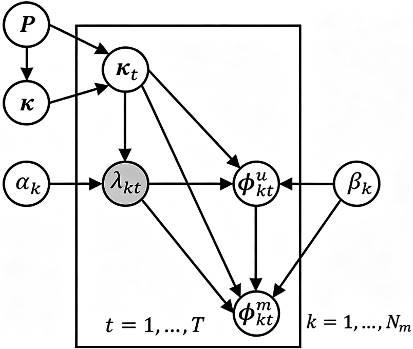
Figure 3. Long description
This flowchart depicts a Bayesian network with nodes labeled P, kappa, alpha sub k, and beta sub k outside a central box. Arrows from P and kappa point to kappa sub t, which is inside the box. Alpha sub k points to lambda sub k t, which is shaded. Kappa sub t and lambda sub k t both point to phi superscript u sub k t and phi superscript m sub k t. Beta sub k points to phi superscript u sub k t. Lambda sub k t also points to phi superscript m sub k t. The box is annotated at the bottom with t equals 1 to T and k equals 1 to N sub m, indicating the range of indices for the variables inside the box.
3. Metropolis-within-Gibbs sampler
To obtain the posterior distribution of unknown parameters in FEMU, we apply the MwG sampling scheme (Li, Reference Li2016; Bardsley and Cui, Reference Bardsley, Cui, de Gier, Praeger and Tao2019) to approximate the posterior in this section. That is, starting from the joint probability distribution in Equation (2.17), the analytical form of the conditional probability distribution of parameters is first derived. Sampling is then implemented from the conditional distribution until convergence is achieved.
3.1. Derivation of MwG sampler
To derive the targeted conditional distributions, we start with the logarithm of the joint distribution in Equation (2.17) by inserting all expressions of PDFs to obtain

The conditional distribution for each of the random variables is then derived by collecting the terms in the joint distribution that include the random variable of interest.
From modal identification, we have the measured mode shape
$ {\boldsymbol{\phi}}_{kt}^m $
 , typically normalized as
$ {{\boldsymbol{\phi}}_{kt}^m}^{\mathrm{T}}{\boldsymbol{\phi}}_{kt}^m=1 $
, typically normalized as
$ {{\boldsymbol{\phi}}_{kt}^m}^{\mathrm{T}}{\boldsymbol{\phi}}_{kt}^m=1 $
 . To sample the latent variable
$ {\boldsymbol{\phi}}_{kt}^u $
. To sample the latent variable
$ {\boldsymbol{\phi}}_{kt}^u $
 , such that
$ \left[{\boldsymbol{\phi}}_{kt}^m;{\boldsymbol{\phi}}_{kt}^u\right] $
, such that
$ \left[{\boldsymbol{\phi}}_{kt}^m;{\boldsymbol{\phi}}_{kt}^u\right] $
 jointly follow a Bingham distribution, we first sample from the conditional distribution of
$ {\boldsymbol{\phi}}_{kt}^u $
jointly follow a Bingham distribution, we first sample from the conditional distribution of
$ {\boldsymbol{\phi}}_{kt}^u $
 given
$ {\boldsymbol{\phi}}_{kt}^m $
given
$ {\boldsymbol{\phi}}_{kt}^m $
 in the Euclidean space, and then project them onto the unit hypersphere. This is valid because the Bingham distribution is essentially a normal distribution projected onto the unit hypersphere. We can obtain the conditional distribution of the latent variable
$ {\boldsymbol{\phi}}_{kt}^u $
in the Euclidean space, and then project them onto the unit hypersphere. This is valid because the Bingham distribution is essentially a normal distribution projected onto the unit hypersphere. We can obtain the conditional distribution of the latent variable
$ {\boldsymbol{\phi}}_{kt}^u $
 by picking up the relevant terms in Equation (3.1) as

where
$ {\boldsymbol{H}}_u\left({\boldsymbol{\kappa}}_t,{\lambda}_{kt}\right) $
 and
$ {\boldsymbol{H}}_m\left({\boldsymbol{\kappa}}_t,{\lambda}_{kt}\right) $
and
$ {\boldsymbol{H}}_m\left({\boldsymbol{\kappa}}_t,{\lambda}_{kt}\right) $
 consist of the columns of
$ \boldsymbol{H}\left({\boldsymbol{\kappa}}_t,{\lambda}_{kt}\right) $
consist of the columns of
$ \boldsymbol{H}\left({\boldsymbol{\kappa}}_t,{\lambda}_{kt}\right) $
 corresponding to the unmeasured and measured DoFs. It indicates that the conditional distribution of
$ {\boldsymbol{\phi}}_{kt}^u $
corresponding to the unmeasured and measured DoFs. It indicates that the conditional distribution of
$ {\boldsymbol{\phi}}_{kt}^u $
 follows a multivariate normal distribution with the precision matrix and the mean vector as


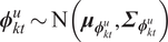
In the MwG sampling, we first sample
$ {\boldsymbol{\phi}}_{kt}^u\sim \mathrm{N}\left({\boldsymbol{\mu}}_{{\boldsymbol{\phi}}_{kt}^u},{\boldsymbol{\varSigma}}_{{\boldsymbol{\phi}}_{kt}^u}\right) $
 and then normalize
$ \left[{\boldsymbol{\phi}}_{kt}^m;{\boldsymbol{\phi}}_{kt}^u\right] $
and then normalize
$ \left[{\boldsymbol{\phi}}_{kt}^m;{\boldsymbol{\phi}}_{kt}^u\right] $
 to have a unit norm.
For conditional distributions
$ p\left(\boldsymbol{\kappa}, \boldsymbol{P}|{\boldsymbol{\kappa}}_{1:T}\right) $
 ,
$ p\left({\alpha}_k|{\boldsymbol{\kappa}}_t,{\lambda}_{k\left(1:T\right)}\right) $
,
$ p\left({\alpha}_k|{\boldsymbol{\kappa}}_t,{\lambda}_{k\left(1:T\right)}\right) $
 , and
$ p\left({\beta}_k|{\boldsymbol{\kappa}}_t,{\lambda}_{k\left(1:T\right)},{\boldsymbol{\phi}}_{k\left(1:T\right)}\right) $
, and
$ p\left({\beta}_k|{\boldsymbol{\kappa}}_t,{\lambda}_{k\left(1:T\right)},{\boldsymbol{\phi}}_{k\left(1:T\right)}\right) $
 , since conjugate priors are assigned for them, their conditional distributions are of the same type as their priors, that is,
$ p\left(\boldsymbol{\kappa}, \boldsymbol{P}|{\boldsymbol{\kappa}}_{1:T}\right)=\mathrm{N}\left(\overline{\boldsymbol{\kappa}},{\left(p\boldsymbol{P}\right)}^{-1}\right)\mathrm{Wishart}\left(\boldsymbol{E},e\right) $
, since conjugate priors are assigned for them, their conditional distributions are of the same type as their priors, that is,
$ p\left(\boldsymbol{\kappa}, \boldsymbol{P}|{\boldsymbol{\kappa}}_{1:T}\right)=\mathrm{N}\left(\overline{\boldsymbol{\kappa}},{\left(p\boldsymbol{P}\right)}^{-1}\right)\mathrm{Wishart}\left(\boldsymbol{E},e\right) $
 ,
$ p\left({\alpha}_k|{\boldsymbol{\kappa}}_t,{\lambda}_{k\left(1:T\right)}\right)=\mathrm{Gam}\left({u}_k,{h}_k\right) $
,
$ p\left({\alpha}_k|{\boldsymbol{\kappa}}_t,{\lambda}_{k\left(1:T\right)}\right)=\mathrm{Gam}\left({u}_k,{h}_k\right) $
 , and
$ p\left({\beta}_k|{\boldsymbol{\kappa}}_t,{\lambda}_{k\left(1:T\right)},{\boldsymbol{\phi}}_{k\left(1:T\right)}\right)=\mathrm{Gam}\left({r}_k,{s}_k\right) $
, and
$ p\left({\beta}_k|{\boldsymbol{\kappa}}_t,{\lambda}_{k\left(1:T\right)},{\boldsymbol{\phi}}_{k\left(1:T\right)}\right)=\mathrm{Gam}\left({r}_k,{s}_k\right) $
 with the following updated hyperparameters


The detailed derivation of the above equations is postponed to Appendix A for simplicity.
All the above conditional distributions belong to a standard family, so that efficient algorithms exist that allow for efficient sample generation. However, this is not the case for the conditional distribution of
$ {\boldsymbol{\kappa}}_t $
 . To see this, collecting terms in Equation (3.1) involving
$ {\boldsymbol{\kappa}}_t $
. To see this, collecting terms in Equation (3.1) involving
$ {\boldsymbol{\kappa}}_t $
 gives
gives

where
$ {\boldsymbol{K}}_{\phi_{kt}}=\left[{\boldsymbol{K}}_1{\boldsymbol{\phi}}_{kt}\hskip0.5em \dots \hskip0.5em {\boldsymbol{K}}_{N_k}{\boldsymbol{\phi}}_{kt}\right]/{\left\Vert {\overline{\lambda}}_k\boldsymbol{M}\right\Vert}_2 $
 and
$ {\boldsymbol{M}}_{\phi_{kt}}=\left({\lambda}_{kt}\boldsymbol{M}{\boldsymbol{\phi}}_{kt}-{\boldsymbol{K}}_0{\boldsymbol{\phi}}_{kt}\right)/{\left\Vert {\overline{\lambda}}_k\boldsymbol{M}\right\Vert}_2 $
and
$ {\boldsymbol{M}}_{\phi_{kt}}=\left({\lambda}_{kt}\boldsymbol{M}{\boldsymbol{\phi}}_{kt}-{\boldsymbol{K}}_0{\boldsymbol{\phi}}_{kt}\right)/{\left\Vert {\overline{\lambda}}_k\boldsymbol{M}\right\Vert}_2 $
 . In order to sample from this conditional distribution, we apply the Metropolis–Hastings (M-H) algorithm (Metropolis et al., Reference Metropolis, Rosenbluth, Rosenbluth, Teller and Teller1953; Hastings, Reference Hastings1970) to asymptotically obtain samples of
$ {\boldsymbol{\kappa}}_t $
. In order to sample from this conditional distribution, we apply the Metropolis–Hastings (M-H) algorithm (Metropolis et al., Reference Metropolis, Rosenbluth, Rosenbluth, Teller and Teller1953; Hastings, Reference Hastings1970) to asymptotically obtain samples of
$ {\boldsymbol{\kappa}}_t $
 .
.
In the M-H algorithm, a proposal distribution has to be selected, which has a crucial role in the performance of the algorithm (Robert and Casella, Reference Robert and Casella1999). To avoid the trouble of tuning the proposal distribution, we propose an independent M-H algorithm considering the structure of the conditional distribution shown in Equation (3.9). More specifically, there are two quadratic terms involving
$ {\boldsymbol{\kappa}}_t $
 , which suggests that we can use a multivariate normal distribution as an independent proposal, and then reject or accept the sample by comparing the remaining terms.
The quadratic terms in Equation (3.9) give a multivariate normal distribution with the precision matrix and mean vector as


It is trivial to sample from such a distribution. Since the sampling does not depend on the current sample
$ {\boldsymbol{\kappa}}_t^{(s)} $
 , it is called an independent proposal.
Once the candidate sample
$ {\boldsymbol{\kappa}}_t^{\left(\ast \right)} $
 are generated; in order to achieve the desired distribution, we accept it with the probability

where we have defined

It can be shown that the proposed independent M-H algorithm satisfies the detailed balance (Robert and Casella, Reference Robert and Casella1999); therefore, it is a valid sampling scheme, that is, it asymptotically converges to the desired distribution. Physically, the second term in Equation (3.13) represents the contribution from the minimum singular value, while the first term captures the effect of the remaining singular values. In terms of magnitude, since modal frequencies can be identified with a high accuracy (Au et al., Reference Au, Brownjohn, Li and Raby2021), the parameter
$ {\alpha}_k $
 is large, leading the second term to dominate. Consequently, the first term can be essentially neglected in computations, leading to
$ \mathcal{D}\left({\boldsymbol{\kappa}}_t\right)\approx \mathcal{D}^{\prime}\left({\boldsymbol{\kappa}}_t\right) $
is large, leading the second term to dominate. Consequently, the first term can be essentially neglected in computations, leading to
$ \mathcal{D}\left({\boldsymbol{\kappa}}_t\right)\approx \mathcal{D}^{\prime}\left({\boldsymbol{\kappa}}_t\right) $
 . A detailed justification for this simplification is provided in Appendix C, and its feasibility will be further validated in the numerical example by comparing results obtained with and without the first term.
An empirical study indicates that the above independent proposal usually generates a very different candidate sample from its seed, leading to a small acceptance rate. To improve sampling efficiency, a scaling parameter
$ \gamma $
 is introduced to adjust the covariance of the proposal distribution as

The step-size tuning parameter
$ \gamma $
 is introduced solely to scale the covariance of this proposal, without altering its mean, thereby controlling the step size and improving the acceptance rate. Since the M-H acceptance formula retains the contribution of the non-quadratic term
$ \mathcal{D}\left({\boldsymbol{\kappa}}_t\right) $
is introduced solely to scale the covariance of this proposal, without altering its mean, thereby controlling the step size and improving the acceptance rate. Since the M-H acceptance formula retains the contribution of the non-quadratic term
$ \mathcal{D}\left({\boldsymbol{\kappa}}_t\right) $
 , the introduction of
$ \gamma $
, the introduction of
$ \gamma $
 does not affect the compensation for the non-quadratic terms, nor does it violate detailed balance or alter the target distribution. Therefore, it enhances sampling efficiency while preserving the theoretical correctness of the sampler. In implementing,
$ \gamma $
does not affect the compensation for the non-quadratic terms, nor does it violate detailed balance or alter the target distribution. Therefore, it enhances sampling efficiency while preserving the theoretical correctness of the sampler. In implementing,
$ \gamma $
 is adaptively determined (Roberts et al., Reference Roberts, Gelman and Gilks1997), as detailed in Section 3.2.
3.2. Robust sampling
Direct sampling from the derived conditional distribution may accumulate numerical errors as it iterates. For example, covariance matrices
$ {\boldsymbol{\varSigma}}_{{\boldsymbol{\phi}}_{kt}^u} $
 ,
$ {\boldsymbol{\varSigma}}_{{\boldsymbol{\kappa}}_t} $
,
$ {\boldsymbol{\varSigma}}_{{\boldsymbol{\kappa}}_t} $
 and
$ \boldsymbol{E} $
and
$ \boldsymbol{E} $
 should be symmetric and positive semi-definite; however, generated samples of them may not always satisfy these requirements. To reduce the possible numerical errors, a robust sampling procedure is developed in this section following the QR decomposition and Cholesky decomposition-based strategies (Wilkinson and Yeung, Reference Wilkinson and Yeung2004).
The conditional distribution
$ p\left({\boldsymbol{\phi}}_{kt}^u|{\boldsymbol{\phi}}_{kt}^m,{\lambda}_{kt},{\kappa}_t,{\beta}_k\right) $
 is a multivariate normal distribution with the precision matrix and the mean vector given in Equations (3.3) and (3.4). In the
$ s $
is a multivariate normal distribution with the precision matrix and the mean vector given in Equations (3.3) and (3.4). In the
$ s $
 -th sampling step, a random sample
$ {{\boldsymbol{\phi}}_{kt}^u}^{\left(s+1\right)} $
-th sampling step, a random sample
$ {{\boldsymbol{\phi}}_{kt}^u}^{\left(s+1\right)} $
 can be generated with the following steps:
1) Take the QR decomposition

2) Draw a sample
$ {\boldsymbol{n}}_{\phi } $
 from a
$ {N}_d-{N}_o $
from a
$ {N}_d-{N}_o $
 dimension standard normal distribution, then

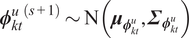
To see
$ {{\boldsymbol{\phi}}_{kt}^u}^{\left(s+1\right)}\sim \mathrm{N}\left({\boldsymbol{\mu}}_{{\boldsymbol{\phi}}_{kt}^u},{\boldsymbol{\varSigma}}_{{\boldsymbol{\phi}}_{kt}^u}\right) $
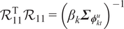
 , one can take the transpose of both sides of Equation (3.15) and then multiply to obtain
$ {\mathcal{R}}_{11}^{\mathrm{T}}{\mathcal{R}}_{11}={\left({\beta}_k{\boldsymbol{\varSigma}}_{{\boldsymbol{\phi}}_{kt}^u}\right)}^{-1} $
, one can take the transpose of both sides of Equation (3.15) and then multiply to obtain
$ {\mathcal{R}}_{11}^{\mathrm{T}}{\mathcal{R}}_{11}={\left({\beta}_k{\boldsymbol{\varSigma}}_{{\boldsymbol{\phi}}_{kt}^u}\right)}^{-1} $
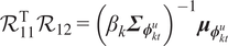
 and
$ {\mathcal{R}}_{11}^{\mathrm{T}}{\mathcal{R}}_{12}={\left({\beta}_k{\boldsymbol{\varSigma}}_{{\boldsymbol{\phi}}_{kt}^u}\right)}^{-1}{\boldsymbol{\mu}}_{{\boldsymbol{\phi}}_{kt}^u} $
and
$ {\mathcal{R}}_{11}^{\mathrm{T}}{\mathcal{R}}_{12}={\left({\beta}_k{\boldsymbol{\varSigma}}_{{\boldsymbol{\phi}}_{kt}^u}\right)}^{-1}{\boldsymbol{\mu}}_{{\boldsymbol{\phi}}_{kt}^u} $
 . With these two equations, one can calculate the covariance of
$ {{\boldsymbol{\phi}}_{kt}^u}^{\left(s+1\right)} $
. With these two equations, one can calculate the covariance of
$ {{\boldsymbol{\phi}}_{kt}^u}^{\left(s+1\right)} $
 as
$ \mathrm{Cov}\left\{{{\boldsymbol{\phi}}_{kt}^u}^{\left(s+1\right)}\right\}={\mathcal{R}}_{11}^{-\mathrm{T}}{\mathcal{R}}_{11}^{-1}/{\beta}_k={\boldsymbol{\varSigma}}_{{\boldsymbol{\phi}}_{kt}^u} $
as
$ \mathrm{Cov}\left\{{{\boldsymbol{\phi}}_{kt}^u}^{\left(s+1\right)}\right\}={\mathcal{R}}_{11}^{-\mathrm{T}}{\mathcal{R}}_{11}^{-1}/{\beta}_k={\boldsymbol{\varSigma}}_{{\boldsymbol{\phi}}_{kt}^u} $
 and the mean of
$ {{\boldsymbol{\phi}}_{kt}^u}^{\left(s+1\right)} $
and the mean of
$ {{\boldsymbol{\phi}}_{kt}^u}^{\left(s+1\right)} $
 as
$ \mathrm{E}\left\{{{\boldsymbol{\phi}}_{kt}^u}^{\left(s+1\right)}\right\}={\mathcal{R}}_{11}^{-1}{\mathcal{R}}_{12}={\boldsymbol{\mu}}_{{\boldsymbol{\phi}}_{kt}^u} $
as
$ \mathrm{E}\left\{{{\boldsymbol{\phi}}_{kt}^u}^{\left(s+1\right)}\right\}={\mathcal{R}}_{11}^{-1}{\mathcal{R}}_{12}={\boldsymbol{\mu}}_{{\boldsymbol{\phi}}_{kt}^u} $
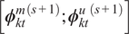
 , satisfying the desired distribution. In addition, we finally normalize
$ \left[{{\boldsymbol{\phi}}_{kt}^m}^{\left(s+1\right)};{{\boldsymbol{\phi}}_{kt}^u}^{\left(s+1\right)}\right] $
, satisfying the desired distribution. In addition, we finally normalize
$ \left[{{\boldsymbol{\phi}}_{kt}^m}^{\left(s+1\right)};{{\boldsymbol{\phi}}_{kt}^u}^{\left(s+1\right)}\right] $
 to have a unit norm.
To sample from the conditional distributions
$ p\left(\boldsymbol{\kappa}, \boldsymbol{P}|{\boldsymbol{\kappa}}_{1:T}\right)=\mathrm{N}\left(\overline{\boldsymbol{\kappa}},{\left(p\boldsymbol{P}\right)}^{-1}\right)\mathrm{Wishart}\left(\boldsymbol{E},e\right) $
 with hypermeters in Equations (3.5) and (3.6), we choose the Cholesky decomposition

By equating the sub-matrices, we have


For the purpose of efficiently sampling
$ \boldsymbol{\kappa} $
 after sampling
$ \boldsymbol{P} $
after sampling
$ \boldsymbol{P} $
 based on the degree of freedom
$ e $
based on the degree of freedom
$ e $
 and
$ {\boldsymbol{L}}_{22} $
and
$ {\boldsymbol{L}}_{22} $
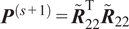
 , we apply the following procedure: Take the Cholesky decomposition
$ {\boldsymbol{P}}^{\left(s+1\right)}={\overset{\sim }{\boldsymbol{R}}}_{22}^{\mathrm{T}}{\overset{\sim }{\boldsymbol{R}}}_{22} $
, we apply the following procedure: Take the Cholesky decomposition
$ {\boldsymbol{P}}^{\left(s+1\right)}={\overset{\sim }{\boldsymbol{R}}}_{22}^{\mathrm{T}}{\overset{\sim }{\boldsymbol{R}}}_{22} $
 , then sample a standard multivariate normal vector
$ {\boldsymbol{n}}_{\kappa}\in {\mathbb{R}}^{N_k} $
, then sample a standard multivariate normal vector
$ {\boldsymbol{n}}_{\kappa}\in {\mathbb{R}}^{N_k} $
 and set

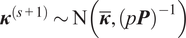
One can verify that
$ {\boldsymbol{\kappa}}^{\left(s+1\right)}\sim \mathrm{N}\left(\overline{\boldsymbol{\kappa}},{\left(p\boldsymbol{P}\right)}^{-1}\right) $
 by computing the mean and covariance.
For the M-H sampling of
$ {\boldsymbol{\kappa}}_t $
 , a robust sampling procedure is implemented to generate a candidate as follows:
1) Perform the Cholesky decomposition
$ \boldsymbol{P}={\boldsymbol{P}}^{\mathrm{T}/2}{\boldsymbol{P}}^{1/2} $
 , where
$ {\boldsymbol{P}}^{\mathrm{T}/2} $
, where
$ {\boldsymbol{P}}^{\mathrm{T}/2} $
 represents the transpose of
$ {\boldsymbol{P}}^{1/2} $
represents the transpose of
$ {\boldsymbol{P}}^{1/2} $
 ;
;
2) Construct the QR decomposition:

3) Draw a sample
$ {\boldsymbol{n}}_{\kappa_t} $
 from a
$ {N}_k $
from a
$ {N}_k $
 -dimension standard normal distribution to obtain a sample following
$ \mathrm{N}\left({\boldsymbol{\mu}}_{{\boldsymbol{\kappa}}_t},{\boldsymbol{\varSigma}}_{{\boldsymbol{\kappa}}_t}\right) $
-dimension standard normal distribution to obtain a sample following
$ \mathrm{N}\left({\boldsymbol{\mu}}_{{\boldsymbol{\kappa}}_t},{\boldsymbol{\varSigma}}_{{\boldsymbol{\kappa}}_t}\right) $
 as
as

Note that
$ {\boldsymbol{\kappa}}_t^{\left(\ast \right)} $
 need to be further screened with the probability given in Equation (3.12). As a summary, the robust implementation of the MwG sampler is listed in Algorithm 1.
Algorithm 1. Robust MwG sampler for FEMU.
Initialization
Choose hyperparameters
$ {\boldsymbol{\kappa}}_0 $
 ,
$ {p}_0 $
,
$ {p}_0 $
 ,
$ {\boldsymbol{E}}_0 $
,
$ {\boldsymbol{E}}_0 $
 ,
$ {e}_0 $
,
$ {e}_0 $
 ,
$ {u}_{k,0} $
,
$ {u}_{k,0} $
 ,
$ {h}_{k,0} $
,
$ {h}_{k,0} $
 ,
$ {r}_{k,0} $
,
$ {r}_{k,0} $
 , and
$ {s}_{k,0} $
, and
$ {s}_{k,0} $

Set
$ {\boldsymbol{\kappa}}_t^{(0)}={\boldsymbol{\kappa}}_0 $
 ,
$ {\boldsymbol{\kappa}}^{(0)}={\boldsymbol{\kappa}}_0 $
,
$ {\boldsymbol{\kappa}}^{(0)}={\boldsymbol{\kappa}}_0 $
 ,
$ {\boldsymbol{P}}^{(0)}={e}_0{\boldsymbol{E}}_0 $
,
$ {\boldsymbol{P}}^{(0)}={e}_0{\boldsymbol{E}}_0 $
 ,
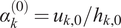
$ {\alpha}_k^{(0)}={u}_{k,0}/{h}_{k,0} $
,
$ {\alpha}_k^{(0)}={u}_{k,0}/{h}_{k,0} $
 and
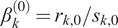
$ {\beta}_k^{(0)}={r}_{k,0}/{s}_{k,0} $
and
$ {\beta}_k^{(0)}={r}_{k,0}/{s}_{k,0} $
For
$ j=1:{N}_{chain} $
 %
$ {N}_{chain} $
%
$ {N}_{chain} $
 denotes the number of MCMC chains, default value of 4
For
$ s=0 $
 to
$ {N}_k-1 $
to
$ {N}_k-1 $
 %
$ {N}_k $
%
$ {N}_k $
 denotes the targeted number of samples in each chain
% 1) Sample
$ {\boldsymbol{\phi}}_{kt}^u $

$ \mathcal{R}=\mathrm{qr}\left(\left[\begin{array}{cc}{\boldsymbol{H}}_u\left({\boldsymbol{\kappa}}_t^{\left(s,j\right)},{\lambda}_{kt}\right)/{\left\Vert {\overline{\lambda}}_k\boldsymbol{M}\right\Vert}_2& -{\boldsymbol{H}}_m\left({\boldsymbol{\kappa}}_t^{\left(s,j\right)},{\lambda}_{kt}\right){\boldsymbol{\phi}}_{kt}^m/{\left\Vert {\overline{\lambda}}_k\boldsymbol{M}\right\Vert}_2\end{array}\right]\right) $
 ;
;
$ {{\boldsymbol{\phi}}_{kt}^u}^{\left(s+1,\mathrm{j}\right)}={\mathcal{R}}_{11}^{-1}\left({\boldsymbol{n}}_{\phi }/\sqrt{\beta_k^{(s)}}+{\mathcal{R}}_{12}\right) $
 where
$ {\boldsymbol{n}}_{\phi}\sim \mathrm{N}\left({\mathbf{0}}_{N_d-{N}_o},{\boldsymbol{I}}_{N_d-{N}_o}\right) $
where
$ {\boldsymbol{n}}_{\phi}\sim \mathrm{N}\left({\mathbf{0}}_{N_d-{N}_o},{\boldsymbol{I}}_{N_d-{N}_o}\right) $
 ;
;
% 2) Sample
$ {\boldsymbol{\kappa}}_t $

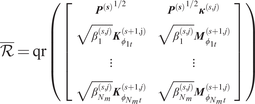
$ \overline{\mathcal{R}}=\mathrm{qr}\left(\left[\begin{array}{c}\begin{array}{cc}{{\boldsymbol{P}}^{\left(\boldsymbol{s}\right)}}^{1/2}& {{\boldsymbol{P}}^{\left(\boldsymbol{s}\right)}}^{1/2}{\boldsymbol{\kappa}}^{\left(s,j\right)}\\ {}\sqrt{\beta_1^{\left(s,j\right)}}{\boldsymbol{K}}_{\phi_{1t}}^{\left(s+1,\mathrm{j}\right)}& \sqrt{\beta_1^{\left(s,j\right)}}{\boldsymbol{M}}_{\phi_{1t}}^{\left(s+1,j\right)}\end{array}\\ {}\begin{array}{cc}\vdots & \vdots \\ {}\sqrt{\beta_{N_m}^{\left(s,j\right)}}{\boldsymbol{K}}_{\phi_{N_mt}}^{\left(s+1,j\right)}& \sqrt{\beta_{N_m}^{\left(s,j\right)}}{\boldsymbol{M}}_{\phi_{N_mt}}^{\left(s+1,j\right)}\end{array}\end{array}\right]\right) $
 ;
;
$ {\boldsymbol{\kappa}}_t^{\left(\ast \right)}={\overline{\mathcal{R}}}_{11}^{-1}\left(\gamma {\boldsymbol{n}}_{\kappa_t}+{\overline{\mathcal{R}}}_{12}\right) $
 where
$ {\boldsymbol{n}}_{\kappa_t}\sim \mathrm{N}\left({\mathbf{0}}_{N_k},{\boldsymbol{I}}_{N_k}\right) $
where
$ {\boldsymbol{n}}_{\kappa_t}\sim \mathrm{N}\left({\mathbf{0}}_{N_k},{\boldsymbol{I}}_{N_k}\right) $
 ;
;
Compute
$ \mathcal{A}\left({\boldsymbol{\kappa}}_t^{\left(s,j\right)},{\boldsymbol{\kappa}}_t^{\left(\ast \right)}\right) $
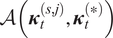 defined in Equation (3.12);
If
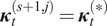
$ \mathcal{A}\left({\boldsymbol{\kappa}}_t^{\left(s,j\right)},{\boldsymbol{\kappa}}_t^{\left(\ast \right)}\right)>\mathrm{Unif}\left(0,1\right) $ $ {\boldsymbol{\kappa}}_t^{\left(s+1,j\right)}={\boldsymbol{\kappa}}_t^{\left(\ast \right)} $
 ; Else
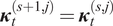
$ {\boldsymbol{\kappa}}_t^{\left(s+1,j\right)}={\boldsymbol{\kappa}}_t^{\left(s,j\right)} $
; Else
$ {\boldsymbol{\kappa}}_t^{\left(s+1,j\right)}={\boldsymbol{\kappa}}_t^{\left(s,j\right)} $
 ; EndIf
% 3) Sample
$ \boldsymbol{\kappa} $
 and
$ \boldsymbol{P} $
and
$ \boldsymbol{P} $

$ \boldsymbol{L}=\mathrm{chol}\left(\left[\begin{array}{cc}{p}_0+T& {\left({p}_0{\boldsymbol{\kappa}}_0+{\sum \limits}_{t=1}^T{\boldsymbol{\kappa}}_t^{\left(s+1,j\right)}\right)}^{\mathrm{T}}\\ {}\left({p}_0{\boldsymbol{\kappa}}_0+{\sum \limits}_{t=1}^T{\boldsymbol{\kappa}}_t^{\left(s+1,j\right)}\right)& {\boldsymbol{E}}_0^{-1}+{p}_0{\boldsymbol{\kappa}}_0{\boldsymbol{\kappa}}_0^{\mathrm{T}}+{\sum \limits}_{t=1}^{\mathrm{T}}{\boldsymbol{\kappa}}_t^{\left(s+1,j\right)}{{\boldsymbol{\kappa}}_t^{\left(s+1,j\right)}}^T\end{array}\right]\right) $
 ;
;
$ {\boldsymbol{P}}^{\left(s+1,j\right)}\sim \mathrm{Wishart}\left(e,{\left({\boldsymbol{L}}_{22}{\boldsymbol{L}}_{22}^T\right)}^{-1}\right) $
 and
$ {\overset{\sim }{\boldsymbol{R}}}_{22}=\mathrm{chol}\left({\boldsymbol{P}}^{\left(s+1,j\right)}{,}^{\prime}\mathrm{uppe}{\mathrm{r}}^{\prime}\right) $
and
$ {\overset{\sim }{\boldsymbol{R}}}_{22}=\mathrm{chol}\left({\boldsymbol{P}}^{\left(s+1,j\right)}{,}^{\prime}\mathrm{uppe}{\mathrm{r}}^{\prime}\right) $
 ;
;
$ {\boldsymbol{\kappa}}^{\left(s+1,j\right)}=\left({\boldsymbol{L}}_{21}+{\overset{\sim }{\boldsymbol{R}}}_{22}^{-1}{\boldsymbol{n}}_{\kappa}\right){L}_{11}^{-1} $
 where
$ {\boldsymbol{n}}_{\kappa}\sim \mathrm{N}\left({\mathbf{0}}_{N_k},{\boldsymbol{I}}_{N_k}\right) $
where
$ {\boldsymbol{n}}_{\kappa}\sim \mathrm{N}\left({\mathbf{0}}_{N_k},{\boldsymbol{I}}_{N_k}\right) $
 ;
;
% 4) Sample
$ {\alpha}_k $
 and
$ {\beta}_k $
and
$ {\beta}_k $

$ {u}_k={u}_{k,0}+\frac{T}{2} $
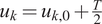 ,
$ {h}_k={h}_{k,0}+\frac{1}{2}\sum_{t=1}^T\frac{\sigma_{\mathrm{min}}^2\left[\boldsymbol{H}\left({\boldsymbol{\kappa}}_t^{\left(s+1,j\right)},{\lambda}_{kt}\right)\right]}{{\left\Vert {\overline{\lambda}}_k\boldsymbol{M}\right\Vert}_2^2} $
,
$ {h}_k={h}_{k,0}+\frac{1}{2}\sum_{t=1}^T\frac{\sigma_{\mathrm{min}}^2\left[\boldsymbol{H}\left({\boldsymbol{\kappa}}_t^{\left(s+1,j\right)},{\lambda}_{kt}\right)\right]}{{\left\Vert {\overline{\lambda}}_k\boldsymbol{M}\right\Vert}_2^2} $
 ;
;
Generate
$ {\alpha}_k^{\left(s+1,j\right)}\sim \mathrm{Gam}\left({u}_k,{h}_k\right) $
 ;
;
$ {r}_k={r}_{k,0}+\frac{T\left({N}_d-1\right)}{2} $
 ,
$ {s}_k={s}_{k,0}+\frac{1}{2}\sum_{t=1}^T{{\boldsymbol{\phi}}_{kt}^{\left(s+1,j\right)}}^T\frac{\boldsymbol{H}{\left({\boldsymbol{\kappa}}_t^{\left(s+1,j\right)},{\lambda}_{kt}\right)}^{\mathrm{T}}\boldsymbol{H}\left({\boldsymbol{\kappa}}_t^{\left(s+1,j\right)},{\lambda}_{kt}\right)}{{\left\Vert {\overline{\lambda}}_k\boldsymbol{M}\right\Vert}_2^2}{\boldsymbol{\phi}}_{kt}^{\left(s+1,j\right)} $
,
$ {s}_k={s}_{k,0}+\frac{1}{2}\sum_{t=1}^T{{\boldsymbol{\phi}}_{kt}^{\left(s+1,j\right)}}^T\frac{\boldsymbol{H}{\left({\boldsymbol{\kappa}}_t^{\left(s+1,j\right)},{\lambda}_{kt}\right)}^{\mathrm{T}}\boldsymbol{H}\left({\boldsymbol{\kappa}}_t^{\left(s+1,j\right)},{\lambda}_{kt}\right)}{{\left\Vert {\overline{\lambda}}_k\boldsymbol{M}\right\Vert}_2^2}{\boldsymbol{\phi}}_{kt}^{\left(s+1,j\right)} $
 ;
;
Generate
$ {\beta}_k^{\left(s+1,j\right)}\sim \mathrm{Gam}\left({r}_k,{s}_k\right) $
 ;
;
Compute the log joint PDF
$ \boldsymbol{Q}\left(j,s+1\right)=\log f\left(\boldsymbol{y},{\boldsymbol{x}}^{\left(s+1,j\right)},{\boldsymbol{\theta}}^{\left(s+1,j\right)}\right) $
 according to Equation (3.1);
EndFor
EndFor
% 5) Convergence criterion—determined by Gelman–Rubin statistic
$ \hat{R} $

For
$ t=100:50:{N}_k $

$ \boldsymbol{\psi} =\boldsymbol{Q}\left(:,t-n+1:t\right) $
 ; %
$ n $
; %
$ n $
 is window length, default value of 100
$ \overline{\boldsymbol{\psi}}=\mathrm{mean}\left(\boldsymbol{\psi} {,}^{\prime}\mathrm{ro}{\mathrm{w}}^{\prime}\right) $
 ;
$ {\overline{\psi}}_{\cdotp \cdotp }=\mathrm{mean}\left(\mathrm{mean}\left(\boldsymbol{\psi} \right)\right) $
;
$ {\overline{\psi}}_{\cdotp \cdotp }=\mathrm{mean}\left(\mathrm{mean}\left(\boldsymbol{\psi} \right)\right) $
 ;
$ \boldsymbol{s}=\operatorname{var}\left(\boldsymbol{\psi} {,}^{\prime}\mathrm{ro}{\mathrm{w}}^{\prime}\right) $
;
$ \boldsymbol{s}=\operatorname{var}\left(\boldsymbol{\psi} {,}^{\prime}\mathrm{ro}{\mathrm{w}}^{\prime}\right) $
 ;
;
Compute within-chain variance
$ W=\frac{1}{N_{chain}\left(n-1\right)}\sum \limits_{j=1}^{N_{chain}}\sum \limits_{i=1}^n{\left(\boldsymbol{\psi} \left(j,i\right)-\overline{\boldsymbol{\psi}}(j)\right)}^2 $
 ;
;
Compute between-chain variance
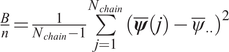
$ \frac{B}{n}=\frac{1}{N_{chain}-1}\sum \limits_{j=1}^{N_{chain}}{\left(\overline{\boldsymbol{\psi}}(j)-{\overline{\psi}}_{\cdotp \cdotp}\right)}^2 $
 ;
;
Estimate the total variance
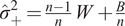
$ {\hat{\sigma}}_{+}^2=\frac{n-1}{n}\;W+\frac{B}{n} $
 ;
;
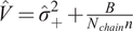
Estimate the pooled posterior variance
$ \hat{V}={\hat{\sigma}}_{+}^2+\frac{B}{N_{chain}n} $
 ;
;
$ {\hat{V}}_d=\frac{{\left(n-1\right)}^2}{n^2{N}_{chain}} \operatorname {var}\left(\boldsymbol{s}\right)+{\left(\frac{N_{chain}+1}{N_{chain}n}\right)}^2\frac{2}{N_{chain}-1}{B}^2+\frac{2\left({N}_{chain}+1\right)\left(n-1\right)}{n^2{N}_{chain}}\bullet \frac{n}{N_{chain}-1}\operatorname{cov}\left(\boldsymbol{s},\left(1-2{\overline{\psi}}_{\cdotp \cdotp}\right)\overline{\boldsymbol{\psi}}\right) $
 ;
;
Calculate the correction coefficient
$ d=2\hat{V}/{\hat{V}}_d $
 ;
$ \delta =\left(d+3\right)/\left(d+1\right) $
;
$ \delta =\left(d+3\right)/\left(d+1\right) $
 ;
;
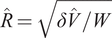
Calculate Gelman-Rubin statistic
$ \hat{R}=\sqrt{\delta \hat{V}/W} $
 ;
;
EndFor
It should be noted that the proposed framework does not assume unimodality of the posterior distribution, while Gibbs sampling often has difficulty in transitioning between different modes efficiently. In principle, multimodality may arise due to limited observations or model nonlinearity. To mitigate this issue, multiple parallel chains with dispersed initializations, together with an annealing scheme, are employed to improve global exploration of the parameter space. Specifically, to avoid prolonged entrapment in local maxima, an annealing scheme is employed (Andrieu et al., Reference Andrieu, de Freitas, Doucet and Jordan2003) by gradually increasing precision parameters
$ \boldsymbol{\alpha} $
 and
$ \boldsymbol{\beta} $
and
$ \boldsymbol{\beta} $
 . As shown in Equations (2.8) and (2.9), the spread of the likelihood strongly depends on the values of precision parameters
$ \boldsymbol{\alpha} $
. As shown in Equations (2.8) and (2.9), the spread of the likelihood strongly depends on the values of precision parameters
$ \boldsymbol{\alpha} $
 and
$ \boldsymbol{\beta} $
and
$ \boldsymbol{\beta} $
 . In order to explore a larger area, these values should be small. Accordingly, within the annealing framework, stage-dependent numerical lower bounds are imposed on two key quantities:
$ {\sum}_{t=1}^T\frac{\sigma_{\mathrm{min}}^2\left[\boldsymbol{H}\left({\boldsymbol{\kappa}}_t^{\left(s+1,j\right)},{\lambda}_{kt}\right)\right]}{{\left\Vert {\overline{\lambda}}_k\boldsymbol{M}\right\Vert}_2^2} $
. In order to explore a larger area, these values should be small. Accordingly, within the annealing framework, stage-dependent numerical lower bounds are imposed on two key quantities:
$ {\sum}_{t=1}^T\frac{\sigma_{\mathrm{min}}^2\left[\boldsymbol{H}\left({\boldsymbol{\kappa}}_t^{\left(s+1,j\right)},{\lambda}_{kt}\right)\right]}{{\left\Vert {\overline{\lambda}}_k\boldsymbol{M}\right\Vert}_2^2} $
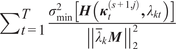 and
$ {\sum}_{t=1}^T{{\boldsymbol{\phi}}_{kt}^{\left(s+1,j\right)}}^T\frac{\boldsymbol{H}{\left({\boldsymbol{\kappa}}_t^{\left(s+1,j\right)},{\lambda}_{kt}\right)}^{\mathrm{T}}\boldsymbol{H}\left({\boldsymbol{\kappa}}_t^{\left(s+1,j\right)},{\lambda}_{kt}\right)}{{\left\Vert {\overline{\lambda}}_k\boldsymbol{M}\right\Vert}_2^2}{\boldsymbol{\phi}}_{kt}^{\left(s+1,j\right)} $
and
$ {\sum}_{t=1}^T{{\boldsymbol{\phi}}_{kt}^{\left(s+1,j\right)}}^T\frac{\boldsymbol{H}{\left({\boldsymbol{\kappa}}_t^{\left(s+1,j\right)},{\lambda}_{kt}\right)}^{\mathrm{T}}\boldsymbol{H}\left({\boldsymbol{\kappa}}_t^{\left(s+1,j\right)},{\lambda}_{kt}\right)}{{\left\Vert {\overline{\lambda}}_k\boldsymbol{M}\right\Vert}_2^2}{\boldsymbol{\phi}}_{kt}^{\left(s+1,j\right)} $
 . These bounds are systematically adjusted based on the current iteration step. Specifically, during the generation of the first 100 samples, a lower-bound constraint is imposed to ensure that the generated values remain within a small range; starting from the 100th step, and at the 300th and 500th steps, this lower bound is reduced by one order of magnitude at each stage, so that its influence gradually diminishes and eventually becomes negligible. This step is carried out during the first 600 iterations. Furthermore, to mitigate the risk of inadequate exploration of the parameter space in sampling, this study adopts a strategy of running
$ {N}_{chain} $
. These bounds are systematically adjusted based on the current iteration step. Specifically, during the generation of the first 100 samples, a lower-bound constraint is imposed to ensure that the generated values remain within a small range; starting from the 100th step, and at the 300th and 500th steps, this lower bound is reduced by one order of magnitude at each stage, so that its influence gradually diminishes and eventually becomes negligible. This step is carried out during the first 600 iterations. Furthermore, to mitigate the risk of inadequate exploration of the parameter space in sampling, this study adopts a strategy of running
$ {N}_{chain} $
 parallel chains. They are initialized by applying a perturbation to each
$ \boldsymbol{\kappa} $
parallel chains. They are initialized by applying a perturbation to each
$ \boldsymbol{\kappa} $
 upon completion of the annealing step. It should be noted that the ideal condition corresponds to the case where the eigenvalue equation is exactly satisfied, that is, the minimum singular value
$ {\sigma}_{\mathrm{min}} $
upon completion of the annealing step. It should be noted that the ideal condition corresponds to the case where the eigenvalue equation is exactly satisfied, that is, the minimum singular value
$ {\sigma}_{\mathrm{min}} $
 approaches zero. Under such conditions, the parameter
$ \boldsymbol{\alpha} $
approaches zero. Under such conditions, the parameter
$ \boldsymbol{\alpha} $
 may become excessively large. To prevent non-physical values, a numerical safeguard is imposed on
$ \boldsymbol{\alpha} $
may become excessively large. To prevent non-physical values, a numerical safeguard is imposed on
$ \boldsymbol{\alpha} $
 after the annealing stage. Specifically, an upper bound is enforced such that
$ \boldsymbol{\alpha} $
after the annealing stage. Specifically, an upper bound is enforced such that
$ \boldsymbol{\alpha} $
 does not exceed a prescribed threshold, which is chosen to be slightly larger than value of
$ \boldsymbol{\alpha} $
does not exceed a prescribed threshold, which is chosen to be slightly larger than value of
$ \boldsymbol{\alpha} $
 obtained at the final iteration of the annealing stage. The specific protection strategy can be adapted depending on the problem under consideration.
To improve sampling efficiency and maintain a reasonable acceptance rate, the proposal scale of the Metropolis step for the stiffness parameters is adaptively tuned during the adaptive proposal tuning stage (1000 iterations directly after the annealing step) of each parallel chain. The specific steps are:
-
0) Monitor the acceptance rate: During the first 1000 iterations, the acceptance rate $ {a}_n $
 is monitored over non-overlapping windows of 100 iterations; if
$ {a}_n\ge 0.2 $
,
$ \gamma =1 $
; Otherwise, do the following.
is monitored over non-overlapping windows of 100 iterations; if
$ {a}_n\ge 0.2 $
,
$ \gamma =1 $
; Otherwise, do the following. -
1) Initialization of step size: Based on the theoretical recommendation of the classical random-walk Metropolis algorithm, the initial step size is set as $ {\gamma}_0=\frac{2.38}{\sqrt{N_k}} $
(Roberts et al., Reference Roberts, Gelman and Gilks1997). -
2) Estimation of the acceptance rate: To suppress short-term stochastic fluctuations, an exponentially smoothed acceptance rate is computed as $ {\bar{a}}_n=\left(1-\delta \right){\bar{a}}_{n-1}+\delta {a}_n $
, where
$ {\bar{a}}_{n-1} $
is initialized to the target acceptance rate
$ {a}^{\ast }=0.2 $
(Roberts et al., Reference Roberts, Gelman and Gilks1997) and
$ \delta $
is a smoothing parameter. The recommended range for
$ \delta $
is between 0.1 and 0.5. -
3) Adaptive step-size adjustment: The proposal scale is updated according to an exponential rule, $ {\gamma}_n={\gamma}_{n-1}\;\exp \left(\eta \left({\bar{a}}_n-{a}^{\ast}\right)\right) $
, where
$ \eta $
is a tuning parameter that adjusts the sensitivity of the step-size update, with values typically chosen between 0.1 and 1. -
4) Fixed-step phase: After the adaptive tuning stage, the step size is held constant for the remaining iterations. At the end of the sampling run, the overall acceptance rate across the entire chain is checked to verify that it remains within a reasonable range.







Finally, convergence of the MwG sampler is assessed by monitoring the evolution of the log joint posterior values (shown in Equation (3.1)) and by applying the corrected Gelman–Rubin diagnostic (Vehtari et al., Reference Vehtari, Gelman, Simpson, Carpenter and Bürkner2021. Multiple parallel chains are used to compare within-chain and between-chain variances. A conservative threshold of
$ \hat{R}<1.05 $
 is adopted to declare convergence. Samples collected after convergence are retained for posterior inference.
The computational cost of the proposed framework primarily arises from two sources: repeated evaluation of the minimum singular value in the likelihood function, and MCMC sampling in a high-dimensional parameter space. Specifically, the use of efficient linear algebra techniques such as QR and Cholesky decompositions enhances numerical efficiency and stability. Additionally, an independent Metropolis–Hastings’s proposal leverages the conditional structure of the problem to improve sampling efficiency. In the following section, we further introduce a model condensation strategy to reduce computational burden and enhance overall efficiency. These strategies collectively reduce the computational burden and make the method applicable to real-world large-scale systems, as illustrated in the empirical studies.
4. Empirical studies
In this section, the performance of the MwG sampler for FEMU is empirically studied through three examples: an 8-DoF mass-spring system, an eight-layer shear-type experimental building model, and a high-rise building—SEG Plaza. The first example illustrates the capability of the proposed method to accurately capture the time variation of the model parameters without modeling errors. The second lab test demonstrates the performance of our method under controllable errors, while the last example verifies the applicability of our algorithm in practical and complex engineering projects.
4.1 8-DoF mass-spring system
First, we consider the numerical example of an 8-DoF mass-spring system, which is an idealization of a real structure and has been previously used by Javier Cara et al. (Reference Javier Cara, Juan, Alarcon, Reynders and De Roeck2013). A schematic diagram of this model is shown in Figure 4. The nominal model parameter values are
$ m=1 $
 and
$ {k}_i=800i $
and
$ {k}_i=800i $
 for
$ i=1,\dots, 9 $
for
$ i=1,\dots, 9 $
 . The true stiffness factor is assumed to have a multivariate normal distribution
$ {\boldsymbol{\kappa}}_t\sim \mathrm{N}\left({\boldsymbol{\mu}}_{\kappa },{\boldsymbol{P}}_{\kappa}^{-1}\right) $
. The true stiffness factor is assumed to have a multivariate normal distribution
$ {\boldsymbol{\kappa}}_t\sim \mathrm{N}\left({\boldsymbol{\mu}}_{\kappa },{\boldsymbol{P}}_{\kappa}^{-1}\right) $
 where
$ {\boldsymbol{\mu}}_{\kappa }={\left[-0.2,-0.15,-0.1,-0.05,0,0.05,0.1,0.15,0.2\right]}^{\mathrm{T}} $
where
$ {\boldsymbol{\mu}}_{\kappa }={\left[-0.2,-0.15,-0.1,-0.05,0,0.05,0.1,0.15,0.2\right]}^{\mathrm{T}} $
 and
$ {\boldsymbol{P}}_{\kappa }=400{\boldsymbol{I}}_9 $
and
$ {\boldsymbol{P}}_{\kappa }=400{\boldsymbol{I}}_9 $
 , that is, the structure is assumed to be time variant with a standard deviation of
$ 0.05 $
, that is, the structure is assumed to be time variant with a standard deviation of
$ 0.05 $
 of
$ {\kappa}_{it} $
of
$ {\kappa}_{it} $
 at each time step. A dataset with a total of
$ T=500 $
at each time step. A dataset with a total of
$ T=500 $
 time steps is generated. In order to synthesize artificial measurements, samples
$ {\boldsymbol{\kappa}}_{1:T} $
time steps is generated. In order to synthesize artificial measurements, samples
$ {\boldsymbol{\kappa}}_{1:T} $
 are generated from
$ \mathrm{N}\left({\boldsymbol{\kappa}}_0,{\boldsymbol{P}}_{\kappa}^{-1}\right) $
are generated from
$ \mathrm{N}\left({\boldsymbol{\kappa}}_0,{\boldsymbol{P}}_{\kappa}^{-1}\right) $
 . The modal frequencies
$ {\lambda}_{kt} $
. The modal frequencies
$ {\lambda}_{kt} $
 and model shapes
$ {\boldsymbol{\phi}}_{kt} $
and model shapes
$ {\boldsymbol{\phi}}_{kt} $
 are then obtained via the generalized eigenvalue decomposition of the assembled mass and stiffness matrices. Finally, measurement errors, modeled as zero-mean Gaussian white noises with variances such that the coefficients of variation of
$ {\lambda}_{kt} $
are then obtained via the generalized eigenvalue decomposition of the assembled mass and stiffness matrices. Finally, measurement errors, modeled as zero-mean Gaussian white noises with variances such that the coefficients of variation of
$ {\lambda}_{kt} $
 and
$ {\boldsymbol{\phi}}_{kt} $
and
$ {\boldsymbol{\phi}}_{kt} $
 are both equal to 0.01, are added. The FEMU problem is to identify
$ \boldsymbol{\kappa} $
are both equal to 0.01, are added. The FEMU problem is to identify
$ \boldsymbol{\kappa} $
 and
$ \boldsymbol{P} $
and
$ \boldsymbol{P} $
 given the “measured” data
$ \left\{{\lambda}_{kt},{\boldsymbol{\phi}}_{kt}^m,k=1,\dots, {N}_m,t=1,\dots, T\right\} $
given the “measured” data
$ \left\{{\lambda}_{kt},{\boldsymbol{\phi}}_{kt}^m,k=1,\dots, {N}_m,t=1,\dots, T\right\} $
 .
.
8-DoFs mass-spring system.

The mass matrix is assumed to be exactly known, so that there is no model error involved in this example. The initial stiffness parameters are selected as
$ {\boldsymbol{\kappa}}_0={\mathbf{0}}_{9\times 1} $
 , that is, we start from the nominal model. Priors for the other hyperparameters, including
$ {p}_0 $
, that is, we start from the nominal model. Priors for the other hyperparameters, including
$ {p}_0 $
 ,
$ {\boldsymbol{E}}_0 $
,
$ {\boldsymbol{E}}_0 $
 ,
$ {e}_0 $
,
$ {e}_0 $
 ,
$ {u}_{k,0} $
,
$ {u}_{k,0} $
 ,
$ {h}_{k,0} $
,
$ {h}_{k,0} $
 ,
$ {r}_{k,0} $
,
$ {r}_{k,0} $
 , and
$ {s}_{k,0} $
, and
$ {s}_{k,0} $
 , are chosen to be non-informative to minimize their impact on the posterior.
We first consider the case using the complete dataset, incorporating all 8 DoFs, all eight modes, and the full set of time steps. As illustrated in Figure 5a, the convergence behavior of the MwG sampler demonstrates rapid stabilization of parameters, indicating that the global optimum is successfully identified shortly after the perturbation. It is worth noting that the acceptance rate of the Metropolis step for updating the stiffness parameters approaches 100%. This behavior is mainly attributed to the construction of an efficient proposal distribution that closely approximates the true conditional posterior of the parameters. By exploiting the conditional Gaussian structure induced by the hierarchical Bayesian formulation, the MwG sampler exhibits Gibbs-like behavior in this numerical example, such that the acceptance probability is largely insensitive to the choice of the step-size parameter
$ \gamma $
 . Therefore, no step-size tuning is required and
$ \gamma =1 $
. Therefore, no step-size tuning is required and
$ \gamma =1 $
 in this example. For posterior analysis, the Gelman–Rubin diagnostic is applied to the four chains. Based on the 1.05 threshold, samples from all four chains, as shown in Figure 5b, are deemed valid for estimating
$ \boldsymbol{\kappa} $
in this example. For posterior analysis, the Gelman–Rubin diagnostic is applied to the four chains. Based on the 1.05 threshold, samples from all four chains, as shown in Figure 5b, are deemed valid for estimating
$ \boldsymbol{\kappa} $
 .
.
Convergence of the MwG sampler; Synthetic data. (a) Iteration process. (b) Gelman-Rubin convergence diagnostic.

Figure 5. Long description
The left panel plots log posterior on the y-axis from 0.94 to 1.08 times 10 to the 4th against iteration on the x-axis from 0 to 4000. Five lines are shown: Chain 1 in blue, Chain 2 in red, Chain 3 in yellow, Chain 4 in purple, and Annealing in green. The green Annealing line starts high and drops sharply before stabilizing, while the four chains overlap closely and remain stable after about iteration 1000. A red ellipse highlights the overlapping region of the four chains between iterations 1000 and 4000, with an inset showing a zoomed view of their fluctuations. The right panel plots Gelman-Rubin index on the y-axis from 0.98 to 1.1 against iteration from 600 to 4000. A blue line fluctuates near 1, always below a red dashed threshold at 1.05, indicating convergence.
To verify the validity of the approximation introduced in Equation (3.13), we compare the posterior distribution of
$ {\boldsymbol{\kappa}}_t $
 between the full expression
$ \mathcal{D}\left({\boldsymbol{\kappa}}_t\right) $
between the full expression
$ \mathcal{D}\left({\boldsymbol{\kappa}}_t\right) $
 (denoted as “Full”) and the approximation
$ \mathcal{D}^{\prime}\left({\boldsymbol{\kappa}}_t\right) $
(denoted as “Full”) and the approximation
$ \mathcal{D}^{\prime}\left({\boldsymbol{\kappa}}_t\right) $
 (denoted as “Approx.”). As shown in Figure 6, the approximation results largely overlap with those obtained from the full setting. This agreement demonstrates the validity of the simplification in Equation (3.13). Consequently, all subsequent computations will adopt this simplified expression.
Influence of full versus approximation of
$ \mathcal{D}\left({\boldsymbol{\kappa}}_t\right) $
 on the posterior distribution of
$ {\boldsymbol{\kappa}}_t $
on the posterior distribution of
$ {\boldsymbol{\kappa}}_t $
 .
.

Figure 6. Long description
Starting at the top left and moving right, then down each row, there are nine panels. Each panel is a line graph with x-axis labeled by a different kappa sub t variable (kappa sub t one to kappa sub t nine) and y-axis labeled P D F. The legend in each panel distinguishes a blue solid line for Approximate and a red dashed line for Full. In every panel, both lines overlap almost perfectly, indicating that the approximate and full posterior distributions are nearly identical for all kappa sub t variables. The x-axis ranges vary slightly per panel, for example, kappa sub t one through kappa sub t three span negative to zero values, while kappa sub t seven through kappa sub t nine include positive values up to about zero point four. The y-axis is consistently scaled from zero to ten. No significant differences are visible between the two methods across all panels.
All
$ \boldsymbol{\kappa} $
 samples throughout the iterations are displayed in Figure 7a. The marginal distributions of parameters
$ {\boldsymbol{\kappa}}_t $
samples throughout the iterations are displayed in Figure 7a. The marginal distributions of parameters
$ {\boldsymbol{\kappa}}_t $
 , plotted in Figure 7b, confirm that the generated samples closely approximate the true distribution
$ \mathrm{N}\left({\boldsymbol{\mu}}_{\kappa },{\boldsymbol{P}}_{\kappa}^{-1}\right) $
, plotted in Figure 7b, confirm that the generated samples closely approximate the true distribution
$ \mathrm{N}\left({\boldsymbol{\mu}}_{\kappa },{\boldsymbol{P}}_{\kappa}^{-1}\right) $
 , shown as a red curve. Furthermore, the correlation coefficients between parameter pairs, shown in Figure 8a, are consistently non-zero, albeit some are close to zero. Similar trends among estimated parameters are also observed in the other cases studied later. These results demonstrate that the proposed method overcomes a key limitation of many traditional approaches, which must assume parameter independence a priori. Instead, our method inherently captures the dependence structure, leading to a more reliable and physically consistent probabilistic model.
Posterior samples; Synthetic data. (a) Samples of κ generated during iterations. (b) Posterior sample distribution of κ t. (with true PDF shown as red curve).

Figure 7. Long description
On the left, a line graph plots kappa on the y-axis from negative 0.2 to positive 0.2 and Iteration on the x-axis from 0 to 4000. Nine colored traces are horizontally aligned, each representing samples of kappa at different levels, showing dense, noisy horizontal bands. On the right, nine small panels are arranged in a 3 by 3 grid. Each panel is a histogram with x-axis labeled kappa sub t and y-axis labeled PDF. The histograms show the distribution of posterior samples for kappa sub t1 through kappa sub t9, with blue bars and a red curve overlay representing the true PDF. The red curve closely follows the histogram bars in each panel, indicating good agreement between the posterior samples and the true distribution.
Correlation coefficients in different cases; Synthetic data. (a) All time data sets. (b) T = 120. (c) DoFs {3,5,6,8}. (d) Modes 1–4.

Figure 8. Long description
Starting at the top-left, panel a shows a nine-by-nine heatmap matrix with kappa one to kappa nine labeled on both axes, representing all time data sets. The diagonal is dark red, indicating a correlation of one, while off-diagonal cells are mostly green and yellow, with some cyan and blue, reflecting lower or negative correlations. The top-right panel b, labeled T equals one hundred twenty, has a similar structure but more cyan and blue off-diagonal cells, indicating more negative correlations. The bottom-left panel c, labeled D o F s three, five, six, eight, shows a similar pattern to panel a but with slightly more yellow and cyan off-diagonal cells. The bottom-right panel d, labeled Modes one to four, also follows this pattern. All panels use a vertical color bar on the right, ranging from negative one in blue to one in red, with zero in green. The main trend is strong self-correlation along the diagonal and variable off-diagonal correlations depending on the case.
To investigate the effect of the data length
$ T $
 on the identified model parameters, we construct six different subsets of data with
$ T=10,50,120,220,350,500 $
on the identified model parameters, we construct six different subsets of data with
$ T=10,50,120,220,350,500 $
 , each comprising the first
$ T $
, each comprising the first
$ T $
 samples. The posterior means and triple standard deviations of
$ \boldsymbol{\kappa} $
samples. The posterior means and triple standard deviations of
$ \boldsymbol{\kappa} $
 are reported in Figure 9 for the considered data subsets. When the number of data is insufficient, a biased posterior distribution can be generated. Under such data-scarce conditions, both the bias and variance of the estimations increase. This behavior indicates that the identifiability of the parameters is reduced when the available data are insufficient. Importantly, the increased posterior variance reflects the lack of information in the data, rather than leading to overconfident or misleading estimates. This phenomenon is further supported by the root mean square (RMS) errors of the means and standard deviations shown in Figure 10a. The convergence of the RMS errors after
$ T=120 $
are reported in Figure 9 for the considered data subsets. When the number of data is insufficient, a biased posterior distribution can be generated. Under such data-scarce conditions, both the bias and variance of the estimations increase. This behavior indicates that the identifiability of the parameters is reduced when the available data are insufficient. Importantly, the increased posterior variance reflects the lack of information in the data, rather than leading to overconfident or misleading estimates. This phenomenon is further supported by the root mean square (RMS) errors of the means and standard deviations shown in Figure 10a. The convergence of the RMS errors after
$ T=120 $
 indicates the required data length for accurate estimation. The correlation coefficients corresponding to this data length are shown in Figure 8b. Data of this length can be collected from monitored structures in a matter of a few hours, although a longer period of data collection is recommended to observe the full range of environmental and ambient variation effects.
Identified
$ \boldsymbol{\kappa} $
 and triple standard deviations with different data lengths; Synthetic data. Note: true value of
$ \boldsymbol{\kappa} $
and triple standard deviations with different data lengths; Synthetic data. Note: true value of
$ \boldsymbol{\kappa} $
 is shown as a red dotted line on the bar chart at
$ T=10 $
is shown as a red dotted line on the bar chart at
$ T=10 $
 .
.

Figure 9. Long description
The horizontal axis is labeled with kappa sub 1 through kappa sub 9. The vertical axis ranges from negative 0.2 to positive 0.2. For each kappa sub i, there are six vertical bars, each color-coded for T equals 10 (blue), 50 (orange), 120 (green), 220 (purple), 350 (cyan), and 500 (brown), as indicated in the legend at the upper left. Each bar shows the estimated kappa value for that T, with black error bars representing triple standard deviations. The bars for kappa sub 1 through kappa sub 4 are negative, kappa sub 5 is near zero, and kappa sub 6 through kappa sub 9 are positive. Overlaid is a red dotted line with red circles, marking the true kappa values at each kappa sub i. The red line increases linearly from negative 0.2 at kappa sub 1 to positive 0.2 at kappa sub 9. The estimated values converge toward the true values as T increases, with error bars shrinking for larger T.
RMS errors of the mean and standard deviations for different cases; Synthetic data. (a) Different data lengths. (b) Different measured DoFs. (c) Different measured modes.

Figure 10. Long description
Panel a at left plots R M S errors percent on the y axis against data length T on the x axis, ranging from 0 to 500. Both mean and standard deviation decrease rapidly as T increases, leveling off near zero. Panel b in the center plots R M S errors percent versus number of measured D o F s N sub 0 from 2 to 8. Both mean and standard deviation decrease as N sub 0 increases, with standard deviation dropping more steeply. Panel c at right plots R M S errors percent versus number of measured modes N sub m from 2 to 8. The mean remains nearly constant, while standard deviation decreases gradually. All panels use black for mean and blue for standard deviation. Panel labels a, b, c are centered below each respective graph.
To evaluate the correction effect of the system, the theoretical mean frequencies and their uncertainties are calculated separately for data subsets of varying time lengths. Based on the posterior distributions of
$ {\boldsymbol{\kappa}}_t $
 obtained under each condition, the corresponding mean frequencies and uncertainties are then obtained through an inverse computation. As shown in Figure 11, accurate stiffness correction coefficients are achieved across all cases, further confirming the method’s adaptability to different data lengths.
Identified frequencies and standard deviations with different data lengths; Synthetic data.

Figure 11. Long description
Starting at the top-left, each panel shows a vertical axis labeled f sub n in hertz and a horizontal axis labeled T. The panels are ordered left to right, top to bottom, for f sub 1 through f sub 8. Each panel displays two data series: black circles for theoretical values and red circles with error bars for computed values. The legend in each panel identifies these series. Across all panels, the computed frequencies closely match the theoretical values, with error bars indicating 3 standard deviations. The x-axis in each panel ranges from 0 to 500. The y-axis ranges are approximately 2.85 to 2.95 for f sub 1, 5.7 to 5.8 for f sub 2, 8.2 to 8.6 for f sub 3, 11.0 to 11.2 for f sub 4, 13.4 to 13.8 for f sub 5, 16.4 to 16.8 for f sub 6, 19.8 to 20.6 for f sub 7, and 24.5 to 25.0 for f sub 8. The error bars are largest at lower T and decrease as T increases, indicating reduced standard deviation with more data. The overall trend shows stable frequency estimates across increasing T.
Measurement limitations and site conditions often make it impractical to capture all DoFs and modes in engineering applications. Therefore, this study further investigates the impact of incomplete measurements on the accuracy of FEMU. In this numerical example, with
$ T=120 $
 and
$ {N}_m=8 $
and
$ {N}_m=8 $
 , we first consider the scenario where only partial DoFs are measured. The results for the identified model parameters under four different subsets of measured DoFs are shown in Figure 12a. These subsets correspond to
$ {N}_o=2,4,6,8 $
, we first consider the scenario where only partial DoFs are measured. The results for the identified model parameters under four different subsets of measured DoFs are shown in Figure 12a. These subsets correspond to
$ {N}_o=2,4,6,8 $
 , with specific measured DoFs being
$ \left\{3,7\right\} $
, with specific measured DoFs being
$ \left\{3,7\right\} $
 ,
$ \left\{3,5,6,8\right\} $
,
$ \left\{3,5,6,8\right\} $
 ,
$ \left\{2-6,8\right\} $
,
$ \left\{2-6,8\right\} $
 and
$ \left\{1-8\right\} $
and
$ \left\{1-8\right\} $
 , respectively. Additionally, the corresponding RMS errors of the identified model parameters are illustrated in Figure 10b, and correlation coefficients are shown in Figure 8c. As shown in Figure 12a, except for the first case where an insufficient number of data points compromises the model’s extrapolation capability, the remaining identification results demonstrate that the algorithm remains insensitive to the partial absence of measured DoFs.
Identified
$ \boldsymbol{\kappa} $
 and triple standard deviations with different cases; Synthetic data. (a) Different measured DoFs. (b) Different measured modes.

Figure 12. Long description
The top panel shows a bar graph with x-axis labeled kappa sub 1 through kappa sub 9 and y-axis ranging from negative 0.2 to 0.2. Four colored bar groups represent [3,7], [3,5,6,8], [2-6,8], and [1-8] as indicated in the legend at the upper left. Each group displays a bar for each kappa value, with error bars indicating triple standard deviation. A red dashed line with open circles overlays the bars, rising from negative 0.2 at kappa sub 1 to about 0.2 at kappa sub 9. The bottom panel is similarly structured, with the legend showing [1-2], [1-4], [1-6], and [1-8]. In the top panel, the case with only two measured DoFs shows larger deviations, while the other partial-DoF cases remain close to the true values. In the bottom panel, the estimates are close to the true values across the different mode subsets, and the variance is relatively insensitive to the number of measured modes. Overall, the updating accuracy improves as the measurement information becomes more complete.
The influence of the number of measured modes,
$ {N}_m $
 , is also studied, with the results presented in Figure 8d, Figure 10c, and Figure 12b. In this scenario, we set
$ T=120 $
, is also studied, with the results presented in Figure 8d, Figure 10c, and Figure 12b. In this scenario, we set
$ T=120 $
 and
$ {N}_0=8 $
and
$ {N}_0=8 $
 , and consider four subsets of measured modes corresponding to the first two, first four, first six, and all eight modes. The results again show that the generated samples converge to the true parameter values, and the estimation variance is largely insensitive to the number of modes utilized. The reason for this is that including more modes reduces the variance of
$ {\boldsymbol{\kappa}}_t $
, and consider four subsets of measured modes corresponding to the first two, first four, first six, and all eight modes. The results again show that the generated samples converge to the true parameter values, and the estimation variance is largely insensitive to the number of modes utilized. The reason for this is that including more modes reduces the variance of
$ {\boldsymbol{\kappa}}_t $
 —as indicated in Equation (3.10)—while having a negligible effect on
$ \boldsymbol{\kappa} $
—as indicated in Equation (3.10)—while having a negligible effect on
$ \boldsymbol{\kappa} $
 . Considering both scenarios, it is observed that accurate updating results are achieved for each data subset, and the effectiveness of the updating method becomes more prominent as the data becomes more complete.
4.2 8-story lab shear-type building model
The second example is an eight-story laboratory shear-type building model, constructed at the Zhejiang University—University of Illinois Urbana-Champaign Institute, Zhejiang University, as shown in Figure 13a. The structure is assembled from custom aluminum components and consists of two main parts: vertical columns and floor plates. The dimensions of the vertical columns are
$ 2\mathrm{mm}\times 20\mathrm{mm}\times 120\mathrm{mm} $
 , while the floor plates measure
$ 350\mathrm{mm}\times 250\mathrm{mm}\times 20\mathrm{mm} $
, while the floor plates measure
$ 350\mathrm{mm}\times 250\mathrm{mm}\times 20\mathrm{mm} $
 . The columns are bolted to the floor plates, and the base plate is rigidly fixed to the ground.
Basic information of the laboratory eight-story shear-type building model. (a) 8-story shear-type building model. (b) FE model (red circles represent sensor locations). (c) Mode shape of the first 12 modes. (d) SV spectrum. (i.e., eigenvalues of power spectral density matrix).

Figure 13. Long description
Top left panel is a photo of an eight-story shear-type building model with cables attached. Top center panel is a finite element schematic of the same building, with nodes labeled 1 to 36 from bottom to top and red circles marking sensor locations at each floor corner. Top right panel displays twelve wireframe diagrams, each numbered 1 to 12, showing mode shapes with red and blue lines for the first twelve vibrational modes; a three-axis orientation marker is at the bottom right. Bottom panel is a line graph with the y-axis labeled SV in g squared per hertz and the x-axis labeled Frequency in hertz, ranging from 0 to 60. Multiple colored lines represent SV spectra, with peaks at various frequencies. Below the x-axis, mode numbers and directions (Y, X, T) are annotated for each peak, indicating the correspondence between spectral features and vibrational modes.
The initial FE model is constructed using three-dimensional Euler beam elements to represent the structure, with a rigid body assumption applied to the floor plates. By treating the four corner points of each floor plate as nodes, the model comprises a total of 36 nodes and 216 DoFs for the entire structure, as illustrated in Figure 13b. According to the above configurations, we can derive the stiffness and mass matrices of the initial FE model. The resulting natural frequencies, obtained through eigenvalue decomposition, are presented in the fourth column of Table 1.
Comparison of FE model responses with measured data; Lab test

Table 1. Long description
The table has twelve rows for measured modes, with columns for measured frequency in hertz, and for F E model results before and after updating. Each model result group includes M A C, frequency in hertz, and F D R in percent. For mode 1, measured frequency is 1.571, before updating M A C is 0.998, frequency 1.546, F D R 1.591, after updating M A C is 0.999, frequency 1.580, F D R minus 0.573. For mode 2, measured frequency is 4.776, before updating M A C is 0.995, frequency 4.586, F D R 3.978, after updating M A C is 0.999, frequency 4.782, F D R minus 0.126. For mode 3, measured frequency is 7.803, before updating M A C is 0.989, frequency 7.473, F D R 4.229, after updating M A C is 0.998, frequency 7.809, F D R minus 0.077. For modes 4 and 5, measured frequency is 10.545, before updating M A C is 0.988, frequency 10.161, F D R 3.641, after updating M A C is 0.995, frequency 10.506, F D R 0.370. For mode 6, measured frequency is 12.944, before updating M A C is 0.959, frequency 12.388, F D R 4.295, after updating M A C is 0.997, frequency 12.915, F D R 0.224. For mode 7, measured frequency is 14.850, before updating M A C is 0.931, frequency 14.250, F D R 4.040, after updating M A C is 0.998, frequency 14.868, F D R minus 0.121. For mode 8, measured frequency is 16.403, before updating M A C is 0.841, frequency 15.627, F D R 4.7311, after updating M A C is 0.994, frequency 16.387, F D R 0.098. For modes 9 and 10, measured frequency is 17.557, before updating M A C is 0.938, frequency 17.560, F D R minus 0.017, after updating M A C is 0.997, frequency 17.569, F D R minus 0.068. For mode 11, measured frequency is 34.327, before updating M A C is 0.943, frequency 30.298, F D R 11.737, after updating M A C is 0.945, frequency 31.467, F D R 8.332. For mode 12, measured frequency is 53.652, before updating M A C is 0.984, frequency 52.170, F D R 2.762, after updating M A C is 0.983, frequency 53.439, F D R 0.397. For most modes, frequencies become closer to the measured values and F D R values decrease; modes 9–10 are an exception with a slight increase in absolute F D R.
Note: All values of “After updating” are calculated at the mean value of
$ {\boldsymbol{\kappa}}_1 $
 .
.
Owing to the rectangular cross-section of the vertical columns, the structure exhibits two orthogonal principal axes: a flexurally weak axis
$ Y $
 and a flexurally strong axis
$ X $
and a flexurally strong axis
$ X $
 . Due to the uniformity of the model, each floor’s four columns are assigned a shared set of stiffness correction parameters, with each set consisting of the moment of inertia about the weak axis / the strong axis, as well as the rotational moment of inertia. The floor slabs, modeled under the rigid-floor assumption from the outset, are not included in the updating process. As a result, a total of 24 unknown stiffness parameters
$ \boldsymbol{\kappa} $
. Due to the uniformity of the model, each floor’s four columns are assigned a shared set of stiffness correction parameters, with each set consisting of the moment of inertia about the weak axis / the strong axis, as well as the rotational moment of inertia. The floor slabs, modeled under the rigid-floor assumption from the outset, are not included in the updating process. As a result, a total of 24 unknown stiffness parameters
$ \boldsymbol{\kappa} $
 are to be identified.
As shown in Figure 13b, sensors are arranged diagonally across all floor plates in the experiment. A total of 16 bi-directional accelerometers are used to measure the acceleration response along both horizontal axes under white noise base motion, with a sampling rate of 256 Hz over a 24-minute period. Based on the fundamental frequency calculated from the FE model, the data are divided into 23 segments by applying a sliding window of 2-minute length with a 1-minute step between consecutive windows. The frequencies and mode shapes for each dataset are then identified using the Bayesian FFT algorithm (Li and Au, Reference Li and Au2019). For each segment, within the 0–60 Hz frequency range, 12 modes are identified, with close modes presented in Band 4 and Band 8. The singular value spectrum and corresponding frequency bands are shown in Figure 13d. Among these, eight weak-axis translational shapes, two strong‑axis translational shapes, and two torsional modes are identified, as labeled in Figure 13d and illustrated in Figure 13c. It should be noted that the complete mode shapes in Figure 13c are computed based on the rigid-floor assumption. Due to significant mode-shape aliasing present in the two sets of close modes, subspace matching (Van Overschee and De Moor, Reference Van Overschee, De Moor, Van Overschee and De Moor1996) is employed for mode-shape correspondence, and the mean frequency within each close-mode band is taken as the representative frequency.
A comparison of FE model responses with measured data before and after the update is provided in Table 1. Here, the frequency difference ratio (FDR) is defined as the relative change of the circular frequency
$ \left[{\omega}_{kt}-{\omega}_{kt,\mathrm{FE}}\right]/{\omega}_{kt} $
 , where
$ {\omega}_{kt,\mathrm{FE}} $
, where
$ {\omega}_{kt,\mathrm{FE}} $
 denotes the corresponding circular frequency of the FE model. In addition, the modal assurance criterion (MAC) is adopted to compare differences in mode shapes. It is defined as the squared cosine angle between the measured mode shape
$ {\boldsymbol{\phi}}_{kt}^m $
denotes the corresponding circular frequency of the FE model. In addition, the modal assurance criterion (MAC) is adopted to compare differences in mode shapes. It is defined as the squared cosine angle between the measured mode shape
$ {\boldsymbol{\phi}}_{kt}^m $
 and the calculated mode shape
$ {\boldsymbol{\phi}}_{kt,\mathrm{FE}} $
and the calculated mode shape
$ {\boldsymbol{\phi}}_{kt,\mathrm{FE}} $
 , that is,
$ {\left[{\boldsymbol{\phi}}_{kt,\mathrm{FE}}^{\mathrm{T}}{\boldsymbol{\phi}}_{kt}^m\right]}^2 $
, that is,
$ {\left[{\boldsymbol{\phi}}_{kt,\mathrm{FE}}^{\mathrm{T}}{\boldsymbol{\phi}}_{kt}^m\right]}^2 $
 . Values closer to 1 indicate a better match. As observed, there are noticeable discrepancies between the modal parameters of the original FE model and those of experimental measurements, indicating the need for model updating.
To reduce the computational cost, improve efficiency, and ensure that the updated structural parameters remain a valid representation of the full model, the Improved Reduction System (IRS) condensation method (Koutsovasilis and Beitelschmidt, Reference Koutsovasilis and Beitelschmidt2008) is employed. This method retains only the translational DoFs corresponding to the measured nodes, resulting in a reduced-DoFs system. The condensation is subsequently applied to the global stiffness matrix, the substructure stiffness matrix, and the mass matrix.
The next step involves identifying the structural parameters using the MwG sampler. The initial values of the unknown stiffness parameters are set to
$ {\boldsymbol{\kappa}}_0={\mathbf{0}}_{24\times 1} $
 , and all measured modes and DoFs are applied. After applying the annealing scheme, random perturbations are added to
$ \boldsymbol{\kappa} $
, and all measured modes and DoFs are applied. After applying the annealing scheme, random perturbations are added to
$ \boldsymbol{\kappa} $
 , generating four new chains; the whole convergence process is shown in Figure 14a. The proposal step size
$ \gamma $
, generating four new chains; the whole convergence process is shown in Figure 14a. The proposal step size
$ \gamma $
 in the MwG sampler is adaptively tuned to achieve an acceptance rate of approximately 20%, leading to stable convergence diagnostics and reliable posterior uncertainty quantification. The Gelman–Rubin convergence diagnostic is then calculated, and the samples after the point indicated by the red circle in Figure 14b are considered valid and used for the posterior analysis of
$ \boldsymbol{\kappa} $
in the MwG sampler is adaptively tuned to achieve an acceptance rate of approximately 20%, leading to stable convergence diagnostics and reliable posterior uncertainty quantification. The Gelman–Rubin convergence diagnostic is then calculated, and the samples after the point indicated by the red circle in Figure 14b are considered valid and used for the posterior analysis of
$ \boldsymbol{\kappa} $
 .
.
Convergence process of MwG sampler; Lab test. (a) Iteration process. (b) Gelman-Rubin convergence diagnostic.

Figure 14. Long description
The left panel is a line graph with x-axis labeled Iteration from 0 to 4000 and y-axis labeled Log posterior from 200 to 700. Four colored lines represent Chain 1, Chain 2, Chain 3, and Chain 4, with a green line for the Annealing stage. The log posterior rises sharply during the Annealing Stage, marked in yellow from iteration 0 to about 700, then stabilizes in the Adaptive Stage, shaded pink from about 700 to 1600. All chains converge and fluctuate around 600 log posterior after 1200 iterations. The legend identifies each chain and the Annealing stage. The right panel is a line graph with x-axis labeled Iteration from 1600 to 4000 and y-axis labeled Gelman-Rubin index from 0.98 to 1.12. The blue line shows the Gelman-Rubin index fluctuating, peaking above 1.1 near iteration 2000, then decreasing and stabilizing near 1. A red dashed horizontal line marks 1.05, and a red circle highlights a value near 1.01 at about iteration 2000.
The converged results for the posterior analysis are shown in Figures 15, 16, and 17. Due to space constraints, Figures 15 and 17 display only every third parameter (out of the total 24) for clarity. The distributions of
$ {\boldsymbol{\kappa}}_t $
 , depicted in histogram plots closely match normal distributions, represented by the solid red curves, with no evidence of multimodality. This observation is consistent with stable convergence across multiple independent chains, as indicated by the Gelman–Rubin diagnostic, suggesting that the posterior distribution is well-behaved under the available data conditions.
Posterior sample distribution of every third
$ {\boldsymbol{\kappa}}_t $
 ; Lab test.

Figure 15. Long description
The layout consists of eight panels in two rows and four columns. Each panel displays a histogram with a blue fill and a smooth red curve overlay. The x-axis labels correspond to every third stiffness parameter: t 3, t 6, t 9, t 12, t 15, t 18, t 21, and t 24, from left to right and top to bottom. The y-axis in all panels is labeled P D F. The histograms show the posterior sample distributions for kappa sub t at each time point. The distributions are unimodal and approximately symmetric, with the peak shifting slightly and the spread increasing for later time points. The overlaid red curves closely follow the histogram shapes, indicating the fitted probability density functions. The range of the x-axis widens from the first to the last panel, reflecting the spread varies among the displayed parameters.
Correlation coefficients; Lab test.

Figure 16. Long description
A square heatmap matrix with both x and y axes labeled kappa one, kappa five, kappa nine, kappa thirteen, kappa seventeen, and kappa twenty-one. Each cell represents a correlation coefficient between corresponding kappa values. The main diagonal from top-left to bottom-right is dark red, indicating a correlation of one. Off-diagonal cells vary in color: yellow and green for moderate positive correlations, cyan and blue for negative correlations, and orange for intermediate values. The color bar at the right maps blue to negative one, green to zero, and red to one. No strong off-diagonal clustering is visible; correlations are distributed without clear block patterns.
Variation of
$ {\boldsymbol{\kappa}}_t $
 over time; Lab test. Note: error bars represent the mean and triple standard deviation of
$ {\boldsymbol{\kappa}}_t $
over time; Lab test. Note: error bars represent the mean and triple standard deviation of
$ {\boldsymbol{\kappa}}_t $
 , while the dark horizontal line indicates the mean of
$ \boldsymbol{\kappa} $
, while the dark horizontal line indicates the mean of
$ \boldsymbol{\kappa} $
 .
.

Figure 17. Long description
There are eight panels arranged in two rows and four columns. Each panel plots kappa sub t for a specific index (t1, t4, t7, t10, t13, t16, t19, t22) on the y-axis against T on the x-axis, ranging from 0 to 23. Each plot displays a colored line representing the mean kappa sub t over time, with vertical error bars at each data point indicating mean plus or minus three times the standard deviation. A dark horizontal line in each panel marks the overall mean kappa for that index. The y-axis range and mean value differ by panel, with some panels centered near zero and others offset positively or negatively. No major trends or shifts are visible; the data in each panel oscillates around the mean line with relatively consistent spread.
From a numerical perspective, all absolute values of
$ \boldsymbol{\kappa} $
 are less than 0.2, ensuring that the stiffness, after parameter correction, still retains its physical significance. Moreover, from a temporal perspective, it shows the variation of identified values of
$ \boldsymbol{\kappa} $
are less than 0.2, ensuring that the stiffness, after parameter correction, still retains its physical significance. Moreover, from a temporal perspective, it shows the variation of identified values of
$ \boldsymbol{\kappa} $
 and
$ {\boldsymbol{\kappa}}_t $
and
$ {\boldsymbol{\kappa}}_t $
 . The uncertainty interval of the posterior estimate for
$ {\boldsymbol{\kappa}}_t $
. The uncertainty interval of the posterior estimate for
$ {\boldsymbol{\kappa}}_t $
 encompasses the true value
$ \boldsymbol{\kappa} $
encompasses the true value
$ \boldsymbol{\kappa} $
 , further validating the proposed algorithm for FEMU.
To verify the performance of the proposed method, parameter values before and after the update are presented in Table 1 for the first time step, that is,
$ T=1 $
 , the results. It is evident that, whether considering results from individual modal data points or from averaged data, the updated FE model is closer to the actual structure than the original FE model. Figure 18 provides a further comparison of the updating effects across all time steps, using the sum of the FDR and (1-MAC) as metrics. The results consistently demonstrate the effectiveness and robustness of our approach in removing model discrepancies and accurately reflecting the true structural behavior. However, there is one exception for Mode 11 (2nd mode in the strong-axis direction), whose frequency and mode shape do not achieve an ideal accuracy after updating. On the one hand, the modal data for the strong-axis direction is relatively limited, making it difficult to achieve reliable parameter identification. On the other hand, as can be seen from the mode shape plot of Mode 11, there is a coupled effect with the rotational direction at the top story, further inducing difficulty in mode shape updating.
Comparison of the updating effects before and after the update over time; Lab test. Note: bar charts comparing the before and after update results are overlaid; this does not indicate a cumulative relationship. |FDR| denotes the absolute value of FDR.

Figure 18. Long description
The chart displays 23 groups of four overlaid vertical bars, one group for each even T value from 1 to 23 on the x axis. The y axis shows absolute F D R in percent, ranging from 0 to 45. Each group contains: a light blue bar for sum of absolute F D R before update, a dark blue bar for sum of absolute F D R after update, an orange bar for sum of one minus M A C before update, and a brown bar for sum of one minus M A C after update. For all T values, the light blue and orange bars are the tallest, while the dark blue and brown bars are shorter, indicating a reduction in both metrics after the update. The legend at the top identifies each color and metric. No cumulative relationship is implied by the overlay.
Due to the limitations of actual measurement conditions, it is often not possible to obtain complete data. Additionally, determining which measurement modes and DoFs to use is a common challenge in FEMU. Therefore, it is imperative to consider the performance of the algorithm under incomplete modal data. In this example, the scenario of incomplete DoFs measurement is first analyzed. Six different test conditions with varying numbers of DoFs are considered, with all modes set for comparison. As shown in Table 2, Case 2 comprises measurement data from all sensors on floors 1, 3, 5, and 7; Case 3 incorporates data from sensors on one side of floors 1, 3, 5, and 7, combined with data from the opposite side of floors 2, 4, 6, and 8; Case 4 uses data from sensors on floors 2, 5, and 8; Case 5 utilizes data from sensors on floors 4 and 8; whereas Case 6 includes all measurement data along the weak-axis direction.
Incomplete data cases; Lab test
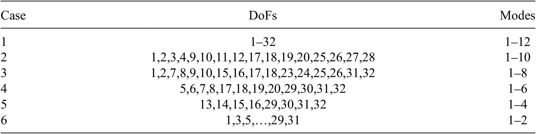
Table 2. Long description
The table has three columns labeled Case, DoFs, and Modes. Row 1: Case 1, DoFs 1 to 32, Modes 1 to 12. Row 2: Case 2, DoFs 1, 2, 3, 4, 9, 10, 11, 12, 17, 18, 19, 20, 25, 26, 27, 28, Modes 1 to 10. Row 3: Case 3, DoFs 1, 2, 7, 8, 9, 10, 15, 16, 17, 18, 23, 24, 25, 26, 31, 32, Modes 1 to 8. Row 4: Case 4, DoFs 5,6,7,8,17,18,19,20,29,30,31,32, Modes 1 to 6. Row 5: Case 5, DoFs 13, 14, 15, 16, 29, 30, 31, 32, Modes 1 to 4. Row 6: Case 6, DoFs 1, 3, 5, up to 29, 31, Modes 1 to 2. DoFs numbering is based on measurement points, with two DoFs per point: weak-axis (odd indices) and strong-axis (even indices). For example, DoFs 1 and 2 correspond to measurement point 1.
Note: DoFs numbering is based on measurement points, with two DoFs per point: weak-axis (odd indices) and strong-axis (even indices). For instance, DoFs 1 and 2 correspond to measurement point 1.
All six cases are identified with the MwG sampler. Figure 19a and b illustrates the comparison of FDR and MAC values across different DoFs. Regarding the model updating results, a reduction in data type or quantity leads to reduced updating performance. One reason for this phenomenon is that the accuracy of mode shape expansion depends heavily on how closely the parameters to be updated approximate their “true values”. Therefore, a lack of information directly undermines the updating capability. This is particularly evident in Case 6: since it only contains complete weak-axis data, the updating performance for strong-axis related modes becomes even worse than that of the original model.
Updating effects under different cases; Lab test. (a) Frequency updates under different measured DoFs. (b) Mode shape updates under different measured DoFs. (c) Frequency updates under different measured modes. (d) Mode shape updates under different measured modes.

Figure 19. Long description
The upper-left and lower-left panels are three-dimensional bar charts with the X-axis representing frequency order, the Y-axis representing case number, and the Z-axis representing absolute F D R percentage. The upper-left panel compares results under different measured D o F cases, while the lower-left panel compares results under different measured-mode cases. Bar colors range from blue to yellow, indicating increasing error magnitude. Overall, as the amount of measurement information decreases, some cases and some frequency orders show noticeably larger absolute F D R values, with higher frequency orders more likely to exhibit larger frequency errors.The upper-right and lower-right panels are also three-dimensional bar charts. The X-axis represents frequency order, the Y-axis represents case number, and the Z-axis represents 1−M A C. The upper-right panel compares results under different measured DoF cases, while the lower-right panel compares results under different measured-mode cases. Bar colors vary from blue to red with increasing frequency order. Overall, the 1−M A C values vary with both case number and frequency order, rather than increasing monotonically for all modes; some intermediate and higher frequency orders exhibit relatively larger mode-shape errors.
Furthermore, six different measured modes with all DoFs conditions are established for comparison. The six subsets are constructed and listed in Table 2. A comprehensive comparison of the updated frequencies and mode shapes is presented in Figure 19c and d. The overall updating performance across all cases is better than that of the original model, indicating that even with limited data under complete measurement DoFs, the model can still effectively constrain parameter updating, especially for weak-axis parameters. A detailed examination reveals that, for modes not used for update, the corresponding frequency correction is noticeably underperformed. Therefore, where conditions permit, using more data contributes to the accuracy and reliability of parameter identification.
To validate the model’s ability to interpret observed data and assess the rationality of time-variant identification, we infer the predictive distributions of frequency responses from the posterior distributions, and compared it with a time-variant two-stage FEMU method (Li et al., Reference Li, He and Liao2026). The results are shown in Figure 20. The analysis reveals that, in terms of mean predictions, the proposed method yields frequency estimates that align more closely with the actual data for most modes. The two‑stage method, however, performs better in correcting the 11th mode frequency, which can be attributed to its likelihood formulation based on minimizing residuals in both frequencies and mode shapes. As for mode shape correction, both methods exhibit comparable performance, which is not presented here for brevity. Regarding uncertainty quantification, the comparison of 99% confidence intervals shows that, compared with the two-stage method, the proposed method not only provides complete coverage of the measured data but also produces intervals with reasonable widths. This effectively alleviates the potential issue of overconfidence that arises from excessively sharp posterior distributions in conventional approaches. The results demonstrate that the proposed method achieves a better trade-off between goodness-of-fit and uncertainty characterization, thereby offering a robust foundation for the subsequent decision-making in damage prognosis.
Comparison of predictive distributions for frequency responses; Lab test.

Figure 20. Long description
Each panel displays the x-axis labeled with a specific frequency response f sub 1 through f sub 12 and the y-axis labeled Normalized P D F. In every panel, the red solid line represents the proposed method, the blue solid line shows the two-stage method, the red dashed line marks the 99 percent confidence interval for the proposed method, the blue dashed line marks the 99 percent confidence interval for the two-stage method, and the green dotted vertical line indicates the measured data. The x-axis values differ per panel, for example, f sub 1 ranges from 1.56 to 1.6, f sub 2 from 4.6 to 4.8, and so on up to f sub 12 from 52 to 56. In most panels, the proposed method (red) produces a wider distribution than the two-stage method (blue), and the measured data (green) is generally centered within the proposed method’s distribution. The confidence intervals for the proposed method are consistently broader than those for the two-stage method. The panels collectively illustrate that the proposed method yields more dispersed predictive distributions, the measured data generally falls within the proposed method’s 99 percent confidence intervals.
4.3 SEG Plaza
In the last example, we consider the FEMU of the SEG Plaza building to verify the effectiveness and applicability of the proposed algorithm in a real-world complex scenario. The SEG Plaza, located in Shenzhen, China, is a 72-story super-tall building (346 meters high), comprising a main tower, a top mast, and a podium, as shown in Figure 21.
On-site photo of the SEG building (Tang et al., Reference Tang, Zhang, Zhou, He, Liu, Chen and Xu2024).

To capture the dynamic characteristics of the structure, a multi-setup ambient vibration test was conducted, consisting of
$ T=12 $
 setups, covering 22 floors with three measurement points on each floor. The first nine experimentally obtained frequencies and mode shapes are shown in Figure 22. Mode shapes are computed using the multi-step Bayesian FFT algorithm (Zhu et al., Reference Zhu, Au, Li and Xie2021) and extended to the full floor plan under the rigid-floor assumption. In the multi-step Bayesian identification, mode shapes are assumed to be invariant across all setups, while frequencies keep changing for each setup. Among the first nine modes, multiple modal forms are present, including translational, torsional, and coupled translational-torsional vibrations. Some close modes (e.g., the 1st and 2nd) exhibit slight modal aliasing. Nonetheless, due to the satisfactory overall modal separation, their frequencies and mode shapes are used independently in the following comparisons. Additionally, due to the limited measurement point, different modes may exhibit similar spatial deformation patterns, as observed in modes 7 and 8. This reflects the significantly asymmetric spatial characteristics of this super high-rise structure.
Measured mode shapes and FE model; Field test. Note: frequency values are identified based on the first setup; X, Y, and T denote translational modes along the weak axis, along the strong axis, and torsional modes, respectively. (a) Mode 1. (b) Mode 2. (c) Mode 3. (d) Mode 4. (e) Mode 5. (f) Mode 6. (g) Mode 7. (h) Mode 8. (i) Mode 9. (j) FE model.

Figure 22. Long description
There are ten panels in a two-row grid. Panels a to i show mode shapes of a tower structure, with each panel labeled above by frequency and mode type: 0.172 Hz 1st Y, 0.172 Hz 1st X, 0.381 Hz 1st T, 0.675 Hz 2nd X, 0.731 Hz 2nd Y, 0.999 Hz 2nd T, 1.291 Hz 3rd X plus T, 1.411 Hz 3rd X plus T, and 1.472 Hz 3rd Y. In each, a wireframe tower is depicted with red and blue lines, indicating measured and finite element (F E) model results. The deformations show bending along the weak axis, strong axis, and twisting, with increasing complexity from left to right and top to bottom. The final panel (j) shows a color-coded F E model with six segments labeled 1 to 6, colored blue to red from bottom to top, and a legend at the center right.
This study adopts a simplified modeling method based on equivalent story stiffness. Through the integration of the existing SAP2000 model, each story of the structure is equivalently represented as a simplified system comprising a floor slab and four identical columns. The top mast section is simplified, with parameters adjusted based on measured modal frequencies. The influence of the podium on the dynamic characteristics of the main structure is approximately simulated by setting spring elements at joints, thereby capturing its mass distribution and stiffness eccentricity effects. The final established FE model consists of 318 nodes and 1,908 DoFs, with its overall geometry illustrated in Figure 22j. Due to the limited information available on the actual structure and the extensive simplifications made in the model, the initial model may exhibit significant discrepancies from the real structure, as listed in Table 3. In terms of frequency deviation, the model exhibits an overall lower stiffness in the weak-axis direction and a generally higher stiffness in the strong-axis direction. Regarding the mode shapes agreement, significant discrepancies are observed in the seventh and eighth modes. Taking the seventh mode as an example, Figure 23a and c compares the measured and FE-computed mode shapes along both principal directions for a set of measurement points that are aligned in plan but at different floor levels. In the weak-axis direction, a fourth-order translational pattern emerges instead of the expected third-order shape. This local difference distinguishes the seventh and eighth modes. In the FE model, it is challenging to simultaneously and precisely capture these two modes with subtle variations.
Modal parameter comparison: initial model, measured data, and condensed model; Field test
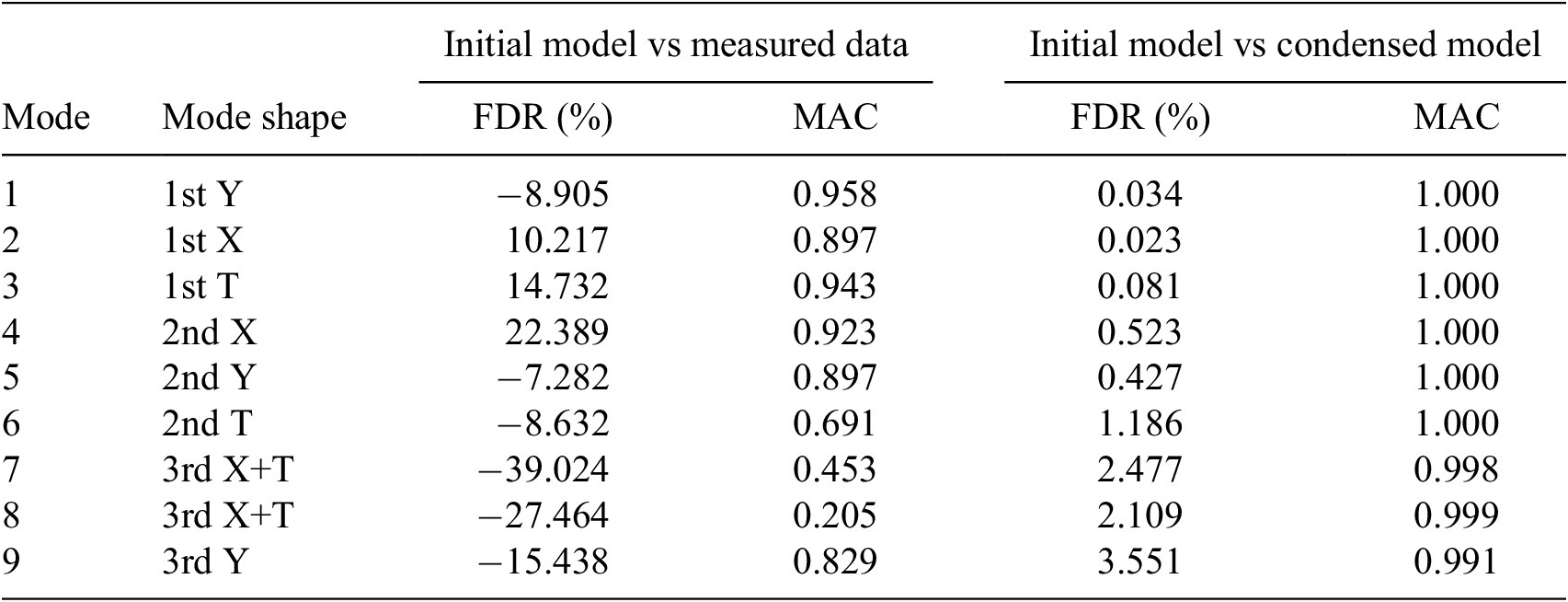
Table 3. Long description
Starting from the top row, Mode 1 with Mode shape 1st Y shows F D R minus 8.905 and M A C 0.958 for initial model vs measured data, F D R 0.034 and M A C 1.000 for initial model vs condensed model. Mode 2, 1st X, has F D R 10.217 and M A C 0.897, then F D R 0.023 and M A C 1.000. Mode 3, 1st T, lists F D R 14.732 and M A C 0.943, then F D R 0.081 and M A C 1.000. Mode 4, 2nd X, shows F D R 22.389 and M A C 0.923, then F D R 0.523 and M A C 1.000. Mode 5, 2nd Y, has F D R minus 7.282 and M A C 0.897, then F D R 0.427 and M A C 1.000. Mode 6, 2nd T, lists F D R minus 8.632 and M A C 0.691, then F D R 1.186 and M A C 1.000. Mode 7, 3rd X plus T, shows F D R minus 39.024 and M A C 0.453, then F D R 2.477 and M A C 0.998. Mode 8, 3rd X plus T, has F D R minus 27.464 and M A C 0.205, then F D R 2.109 and M A C 0.999. Mode 9, 3rd Y, lists F D R minus 15.438 and M A C 0.829, then F D R 3.551 and M A C 0.991. Across all modes, M A C values for initial model vs condensed model are close to 1.000, indicating high correlation, while F D R values vary, with negative values in some modes and positive in others.
Comparison between measured and FE mode shapes before and after update; Field test. (a) Weak axis mode shape before update. (b) Weak axis mode shape after update. (c) Strong axis mode shape before update. (d) Strong axis mode shape after update.

Figure 23. Long description
Top-left panel shows weak-axis mode shape before update with layer height in meters on the y-axis and mode shape on the x-axis from minus one to one. Blue circles labeled F E M and red circles labeled Data diverge, especially above 100 meters. Top-right panel shows weak-axis mode shape after update; blue and red circles align closely throughout the height. Bottom-left panel shows strong-axis mode shape before update; blue and red circles diverge above 100 meters. Bottom-right panel shows strong-axis mode shape after update; blue and red circles are nearly coincident across all heights. All panels are labeled Mode 7 and include a legend indicating F E M and Data.
Based on the arrangement of measurement points and the structural characteristics, the structure is divided into six main stiffness zones, as shown in Figure 22j, where different correction zones are distinguished by distinct colors. The mast section and the spring elements that represent the podium are excluded from the updating process, because there is no measurement point on them. For each zone, the vertical columns share the same set of stiffness correction parameters for strong- and weak-axis moments of inertia, resulting in a total of 12 unknown parameters. A relatively small number of parameters is considered here because the primary objective in this study is to verify whether the proposed algorithm can effectively yield a model better aligned with the measured responses.
Considering that the simplified model still retains a large number of DoFs, model condensation is employed using the IRS method. In the condensation setup, translational DoFs corresponding to measurement points are defined as master DoFs, yielding 189 DoFs in total. Table 3 presents the differences in modal frequencies and mode shapes before and after condensation, showing good consistency in mode shapes for the first nine modes. Although certain errors exist in higher-order frequencies, these errors remain at a relatively low level compared to those of the initial model. Therefore, the reduced model will be used for subsequent updates.
The MwG sampler is then adopted to update the condensed FE model. Figure 24a and b displays the log posterior and the Gelman-Rubin statistic during the iterative process. The posterior distributions of stiffness parameters are provided in Figure 25, where the dark horizontal line represents the identified mean value of
$ \boldsymbol{\kappa} $
 , while the error bars indicate the mean and triple standard deviation of
$ {\boldsymbol{\kappa}}_t $
, while the error bars indicate the mean and triple standard deviation of
$ {\boldsymbol{\kappa}}_t $
 identified at each setup. Regarding the identified values of
$ \boldsymbol{\kappa} $
identified at each setup. Regarding the identified values of
$ \boldsymbol{\kappa} $
 , the parameters associated with the weak axis are all positive, while those related to the strong axis are all negative. This outcome aligns with the initial judgment: the initial stiffness is generally lower in the weak-axis direction and higher in the strong-axis direction. Therefore, positive and negative correction parameters can effectively compensate for frequency errors in the respective directions. The updated mode shape of Mode 7 is shown in Figure 23b and d. In terms of physical meaning, since a rough model is used as an initial reference, the identified relatively large positive values are still acceptable; negative parameters carry clear physical significance and are likewise within a reasonable range. From the mean values and uncertainties of the identified
$ {\boldsymbol{\kappa}}_t $
, the parameters associated with the weak axis are all positive, while those related to the strong axis are all negative. This outcome aligns with the initial judgment: the initial stiffness is generally lower in the weak-axis direction and higher in the strong-axis direction. Therefore, positive and negative correction parameters can effectively compensate for frequency errors in the respective directions. The updated mode shape of Mode 7 is shown in Figure 23b and d. In terms of physical meaning, since a rough model is used as an initial reference, the identified relatively large positive values are still acceptable; negative parameters carry clear physical significance and are likewise within a reasonable range. From the mean values and uncertainties of the identified
$ {\boldsymbol{\kappa}}_t $
 , the model successfully captures the variability arising from environmental factors and the inherent structural characteristics. This variability is largely due to the modeling error, which helps explain the dispersion observed in the measured data.
Convergence of the MwG sampler; Field test. (a) Iteration process. (b) Gelman-Rubin convergence diagnostic.

Figure 24. Long description
The left panel plots log posterior on the y-axis from negative 100 to 200 against iteration on the x-axis from 0 to 4000. Four colored lines represent Chain 1 in blue, Chain 2 in red, Chain 3 in yellow, and Chain 4 in purple. An additional green line labeled Annealing appears in the early iterations. The background is divided into two shaded regions: a yellow region labeled Annealing Stage from iteration 0 to about 600, and a pink region labeled Adaptive Stage from about 600to 1600. After these stages, all chains converge and fluctuate around zero log posterior. The legend is centered in the plot area. The right panel plots Gelman-Rubin index on the y-axis from 0.98 to 1.12 against iteration on the x-axis from 1600 to 4000. A blue line shows the index fluctuating between 1 and 1.05, with a red dashed horizontal line at 1.05. A red circle marks the initial value near 1.02. The index remains below the threshold throughout.
Variation of
$ {\boldsymbol{\kappa}}_t $
 over time; Field test. Note: error bars represent the mean and triple standard deviation of
$ {\boldsymbol{\kappa}}_t $
over time; Field test. Note: error bars represent the mean and triple standard deviation of
$ {\boldsymbol{\kappa}}_t $
 , while the dark horizontal line indicates the mean of
$ \boldsymbol{\kappa} $
, while the dark horizontal line indicates the mean of
$ \boldsymbol{\kappa} $
 . “
$ T $
. “
$ T $
 ” denotes the number of test setups.

Figure 25. Long description
From top left to bottom right, each panel is labeled kappa sub t1 through kappa sub t12 on the y-axis and T on the x-axis, ranging from 0 to 12. Each graph displays colored data points with vertical error bars representing the mean and triple standard deviation of kappa sub t at each T value. A dark horizontal line marks the mean kappa value for each panel. The y-axis range and data distribution differ per panel: for example, kappa sub t1 ranges from 0.7 to 0.8, kappa sub t5 from 2.2 to 2.6, and kappa sub t6 from -0.25 to -0.05. Most panels show stable trends with overlapping error bars and little systematic change across T. All axes and labels use italicized Greek and Latin letters as shown.
Figure 26 illustrates the performance of the proposed MwG sampler by comparing the updated modal data, using the mean value of the first setup as an example. Here, the first nine modes are used as the measured data for updates. Therefore, it is no wonder that the overall frequency and mode shape errors are significantly reduced, although several modes still exhibit discrepancies. This is likely due to the oversimplification of the model, which stems from the trade-off between missing substantial physical information and the need for computational efficiency. In addition, modal data from Modes 10–15 are also investigated to examine the generalization capacity of the updated model, because these data are not used in the updating process. The significant reduction of errors in these modes indicates that the updated model aligns much better with the actual structural behavior. Future refinements may involve introducing additional unknown parameters, comparing different model configurations to establish an optimization path, and balancing the trade-off between model complexity and accuracy.
Comparison of the updating effects before and after the update; Field test. (a) Frequencies. (b) Mode shapes.

Figure 26. Long description
The top panel plots F D R percentage on the y-axis and Mode on the x-axis, with blue bars for F D R before update and green bars for F D R after update. Most modes show a reduction in F D R after update, especially at modes 7, 8, 11, and 13, where blue bars are much higher or lower than green. The bottom panel plots one minus M A C on the y-axis and Mode on the x-axis, with orange bars for before update and yellow bars for after update. After update, one minus M A C values decrease for most modes, especially at modes 7, 8, 11, 12, and 13, indicating improved mode shape correlation. Legends are present in both panels, and all axes are labeled.
5. Conclusion and discussion
This paper presents a hierarchical Bayesian framework for FEMU that explicitly accounts for time-varying structural properties, a critical factor for handling uncertainties due to environmental and operational conditions. By treating unmeasured mode shapes as latent variables and constructing the likelihood function directly from eigen-equation residuals, the proposed method eliminates the need for tedious modal matching and computationally expensive eigenvalue decomposition, while naturally preserving the physical interpretability of the updated model. The proposed method is validated through empirical studies on an 8-DoF mass-spring system, an eight-story lab shear-type building model, and SEG Plaza. The main conclusions are as follows:
-
(1) The developed hierarchical Bayesian framework can explicitly characterize the time-varying behavior of structural parameters, enabling robust and uncertainty-aware identification in dynamic systems.
-
(2) A smallest-singular-value-based residual formulation is introduced to alleviate numerical ill-conditioning and enhance computational stability in high-dimensional problems; Mode shapes are modeled on the unit hypersphere using a Bingham distribution, which naturally enforces their intrinsic geometric constraints.
-
(3) The employed MwG sampling strategy can effectively infer the joint distribution of structural parameters and latent modal shapes, providing accurate posterior estimation without repeated eigenvalue decomposition.
It should be acknowledged that the FEMU of real-world, complex engineering structures is challenging due to the imbalance of the complicated model and limited data, typically featuring a multi-modal high-dimensional likelihood. The proposed method provides a step forward toward robust identification, but still shows inadequacy in addressing complicated examples, which require not only advanced identification methods but also a good initial model and careful selection of updating parameters. In the future, we will combine the Bayesian model selection technique to balance the model complexity and accuracy, while designing a more efficient sampling strategy to explore multimodal posteriors arising from insufficient data.
Data availability statement
The synthetic and laboratory test data supporting this study are openly available at https://doi.org/10.7910/DVN/C8ZRHY (Li et al., Reference Li, Liao and Zhu2025a). However, the field test data are not publicly accessible due to contractual restrictions. All MATLAB codes are available at https://github.com/Mingzhu-Chen/Matlab-code-for-MwG.
Author contribution
M.C.: conceptualization, formal analysis, investigation, methodology, software, validation, visualization, writing – original draft, writing – review & editing; B.L.: conceptualization, data curation, formal analysis, funding acquisition, investigation, methodology, project administration, resources, software, supervision, validation, visualization, writing – original draft, writing – review & editing; A.D.K.: conceptualization, formal analysis, investigation, methodology, resources, supervision, writing – review & editing; C.Q.: funding acquisition, investigation, project administration, resources, supervision, writing – review & editing.
Funding statement
The author(s) disclose receipt of the following financial support for the research, authorship, and/or publication of this article: the National Natural Science Foundation of China [Grant numbers 52561145240 and 52222807].
Competing interests
The author(s) declared no potential conflicts of interest with respect to the research, authorship, and/or publication of this article.
Appendix A
Table A1 lists the abbreviations and their definitions used throughout this paper
List of abbreviations
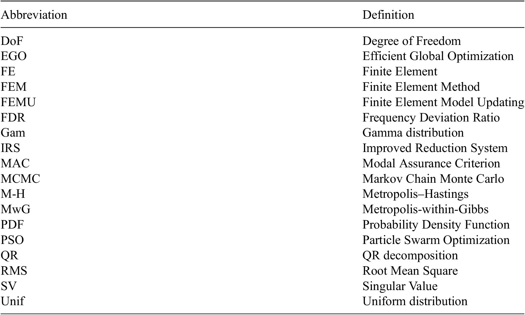
Table A1. Long description
Starting from the top row, the left column contains abbreviations and the right column provides their definitions. The entries are: DoF for Degree of Freedom, EGO for Efficient Global Optimization, FE for Finite Element, FEM for Finite Element Method, FEMU for Finite Element Model Updating, FDR for Frequency Deviation Ratio, Gam for Gamma distribution, IRS for Improved Reduction System, MAC for Modal Assurance Criterion, MCMC for Markov Chain Monte Carlo, M-H for Metropolis–Hastings, MwG for Metropolis-within-Gibbs, PDF for Probability Density Function, PSO for Particle Swarm Optimization, QR for QR decomposition, RMS for Root Mean Square, SV for Singular Value, and Unif for Uniform distribution. Each abbreviation is paired with its definition in a horizontal row, proceeding sequentially from the top to the bottom of the table.
Appendix B
We provide the detailed derivation for conditional distributions used in the MwG sampler in this appendix.
First, for the conditional distribution of
$ \boldsymbol{\kappa} $
 and
$ \boldsymbol{P} $
and
$ \boldsymbol{P} $
 , since a conjugate normal-Wishart prior has been assigned, their conditional distribution is expected to be the normal-Wishart as well. To see this, collecting the terms involving
$ \boldsymbol{\kappa} $
, since a conjugate normal-Wishart prior has been assigned, their conditional distribution is expected to be the normal-Wishart as well. To see this, collecting the terms involving
$ \boldsymbol{\kappa} $
 and
$ \boldsymbol{P} $
and
$ \boldsymbol{P} $
 in Equation (3.1) gives

in which we have

Second, for conditional distributions of
$ {\boldsymbol{\alpha}}_{\boldsymbol{k}} $
 and
$ {\boldsymbol{\beta}}_{\boldsymbol{k}} $
and
$ {\boldsymbol{\beta}}_{\boldsymbol{k}} $
 , the situation is similar to the above because conjugate priors are assigned to them, too. Specifically, we have

where

The conditional distribution of
$ {\beta}_k $
 can be obtained as

where

Appendix C
Under continuous structural health monitoring, modal frequencies are repeatedly measured with a high signal-to-noise ratio. As a consequence, the precision parameter
$ {\alpha}_k $
 associated with the eigenvalue equation constraint typically attains large but finite values.
The Metropolis–Hastings acceptance ratio for sampling
$ {\boldsymbol{\kappa}}_t $
 depends on

where

and terms independent of
$ {\boldsymbol{\kappa}}_t $
 have been omitted.
Let
$ {\boldsymbol{\kappa}}_t^{\ast } $
 denote a configuration satisfying the eigenvalue equation constraint in a noise-free sense

The smallest singular value admits a second-order local approximation

where
$ {\mathbf{Y}}_k $
 is a positive semi-definite curvature matrix.
Meanwhile, the pseudo-determinant term involves only the non-vanishing singular values and is therefore smooth in the same neighborhood.

with
$ {\boldsymbol{g}}_k $
 denoting a bounded gradient with respect to
$ {\boldsymbol{\kappa}}_t $
denoting a bounded gradient with respect to
$ {\boldsymbol{\kappa}}_t $
 evaluated at
$ {\boldsymbol{\kappa}}_t^{\ast } $
evaluated at
$ {\boldsymbol{\kappa}}_t^{\ast } $
 .
.
In the large-precision regime (
$ {\alpha}_k\gg 1 $
 ), the posterior density strongly penalizes deviations from eigen-consistent configurations. Hence, the Markov chain predominantly explores a neighborhood of
$ {\boldsymbol{\kappa}}_t^{\ast } $
), the posterior density strongly penalizes deviations from eigen-consistent configurations. Hence, the Markov chain predominantly explores a neighborhood of
$ {\boldsymbol{\kappa}}_t^{\ast } $
 in which the quadratic penalty remains of moderate magnitude

Using the second-order approximation, this condition implies the characteristic scale.

Importantly, this scaling reflects posterior concentration due to large but finite precision, rather than an asymptotic limit. Substituting the scaling into the local expansion (C.5) yields

Therefore, within the region effectively explored by the Markov chain,

where the second
$ O\left({\alpha}_k^{-1/2}\right) $
 term becomes negligible for sufficiently large
$ {\alpha}_k $
term becomes negligible for sufficiently large
$ {\alpha}_k $
 .
.
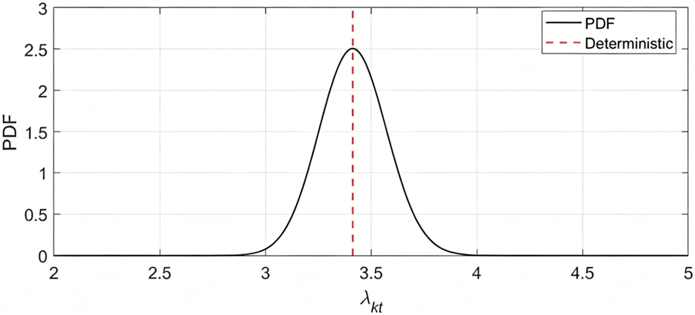
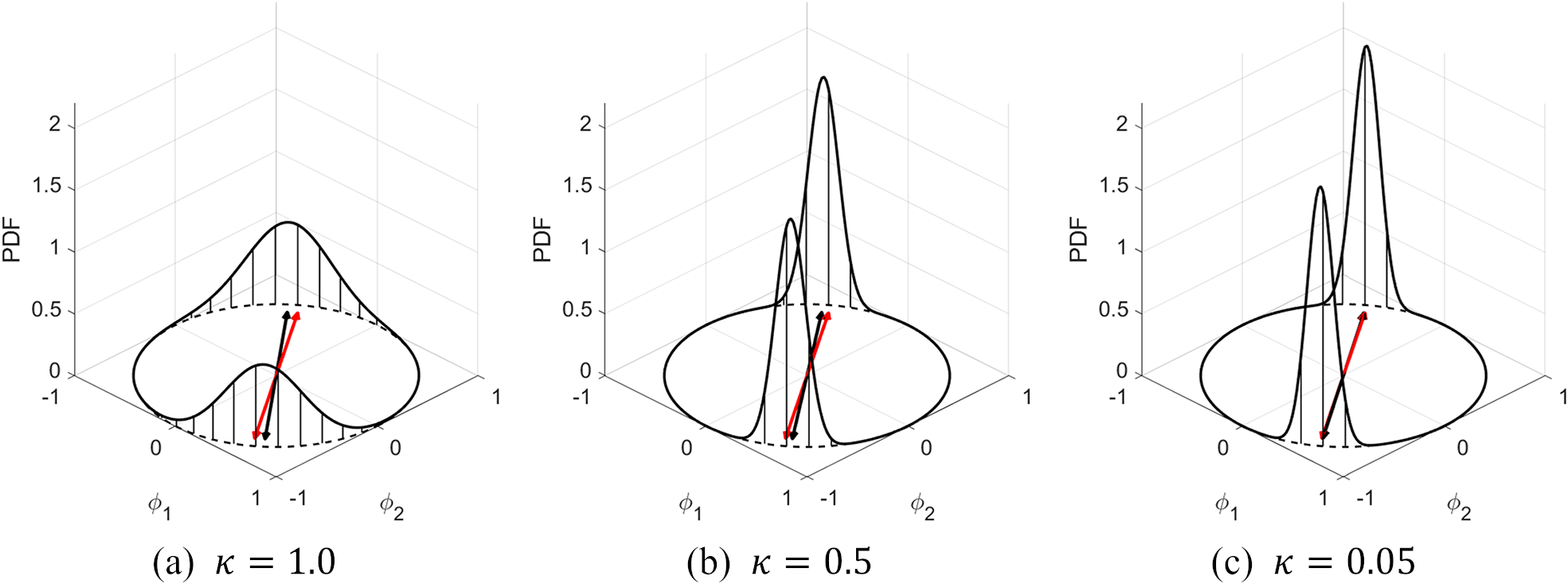

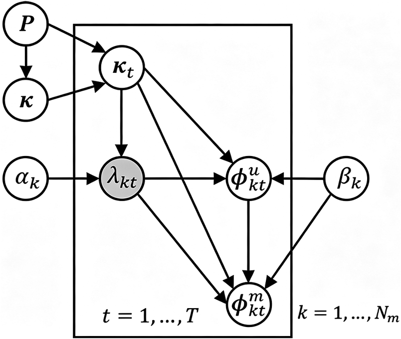

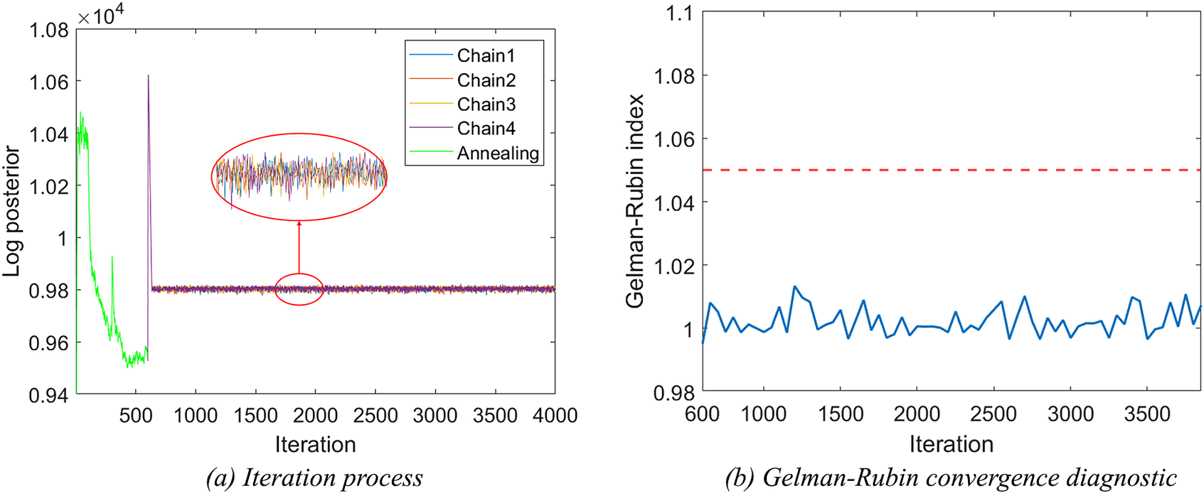
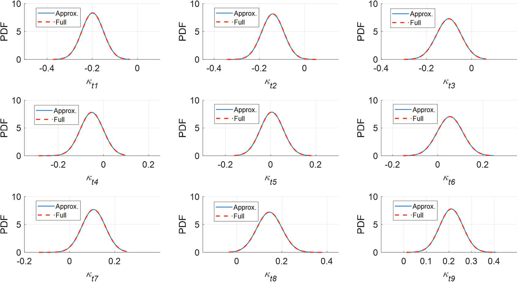


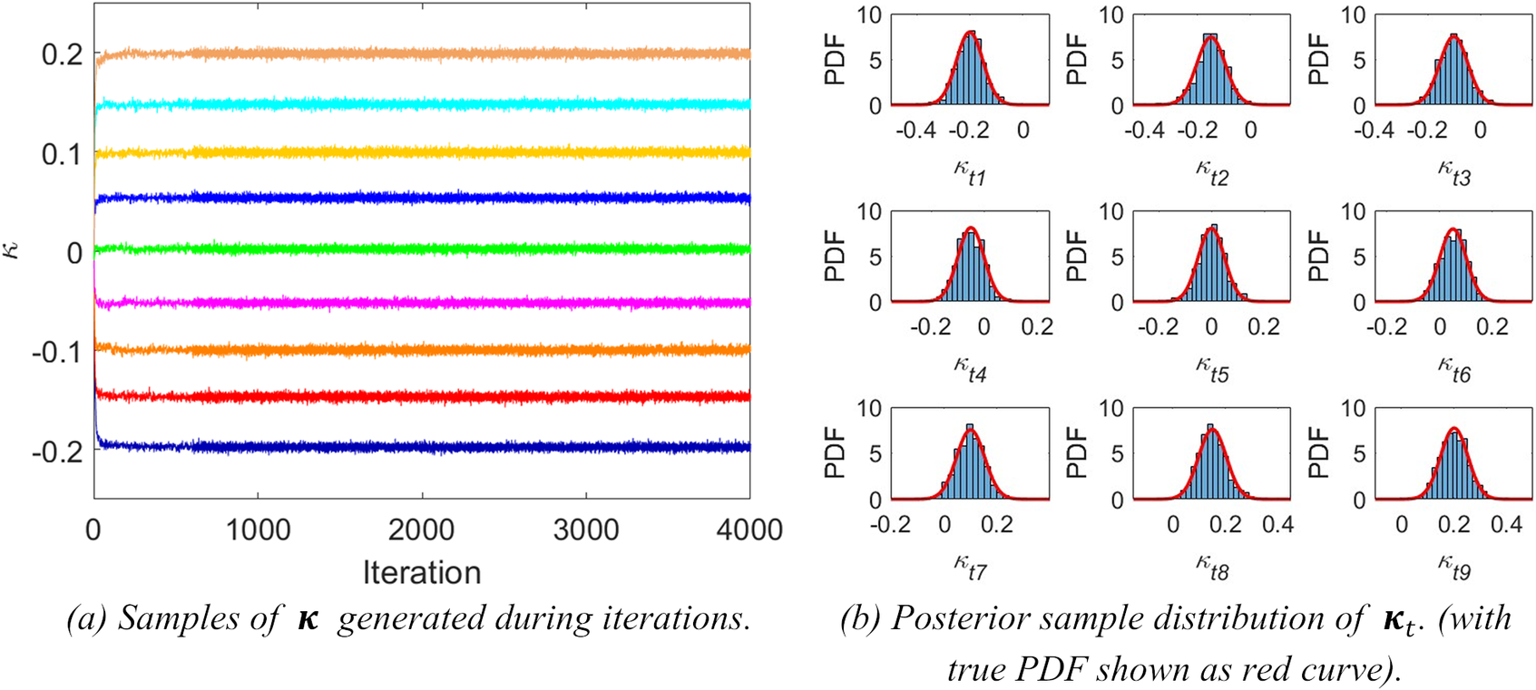
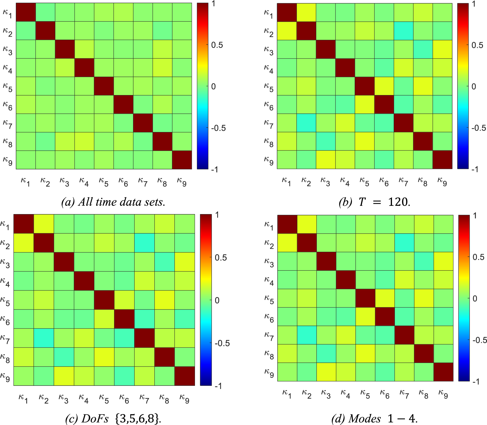
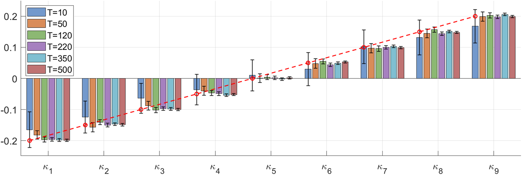


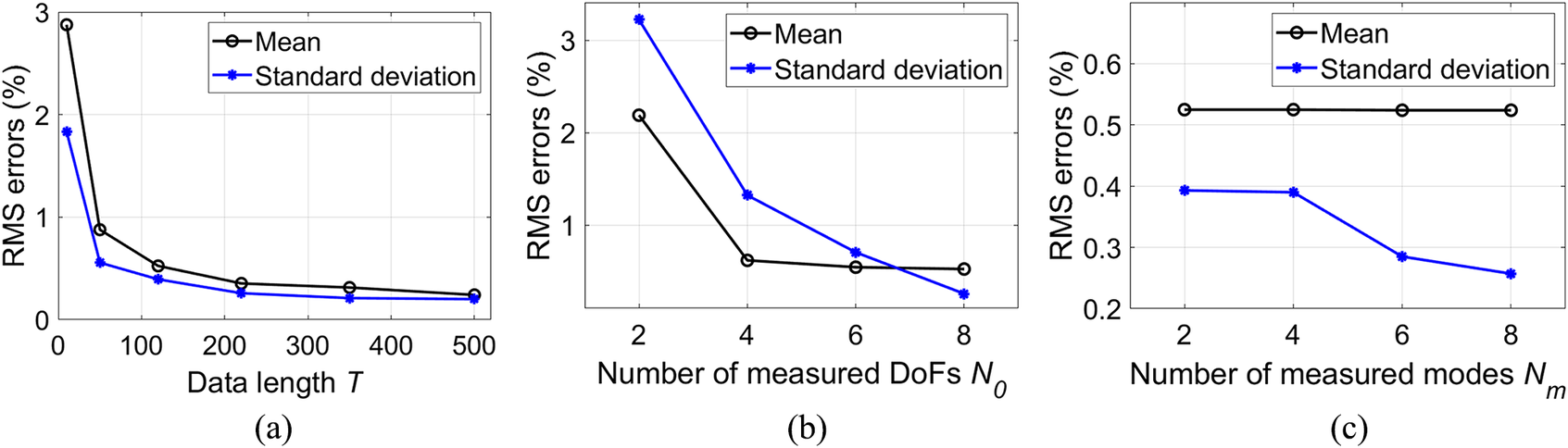
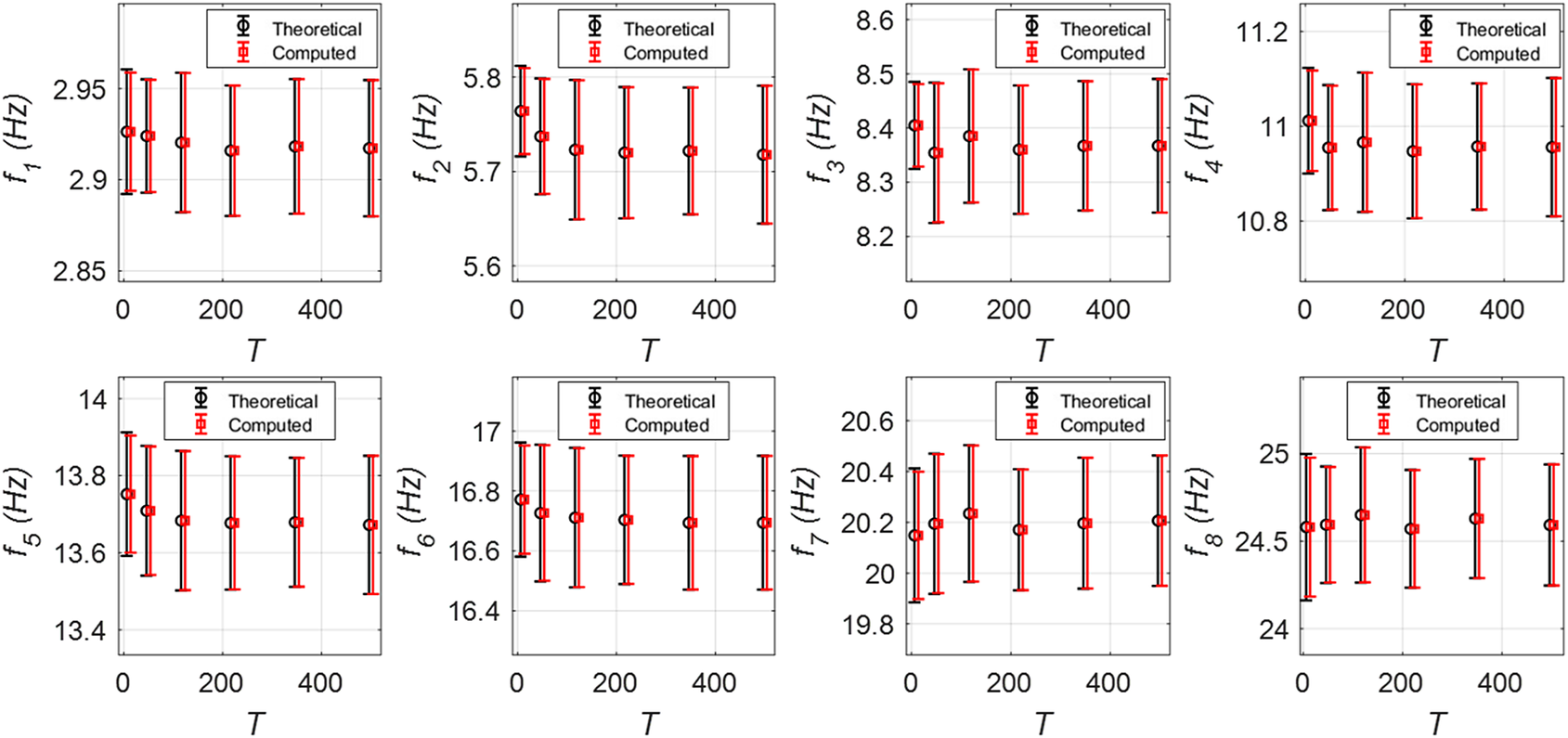
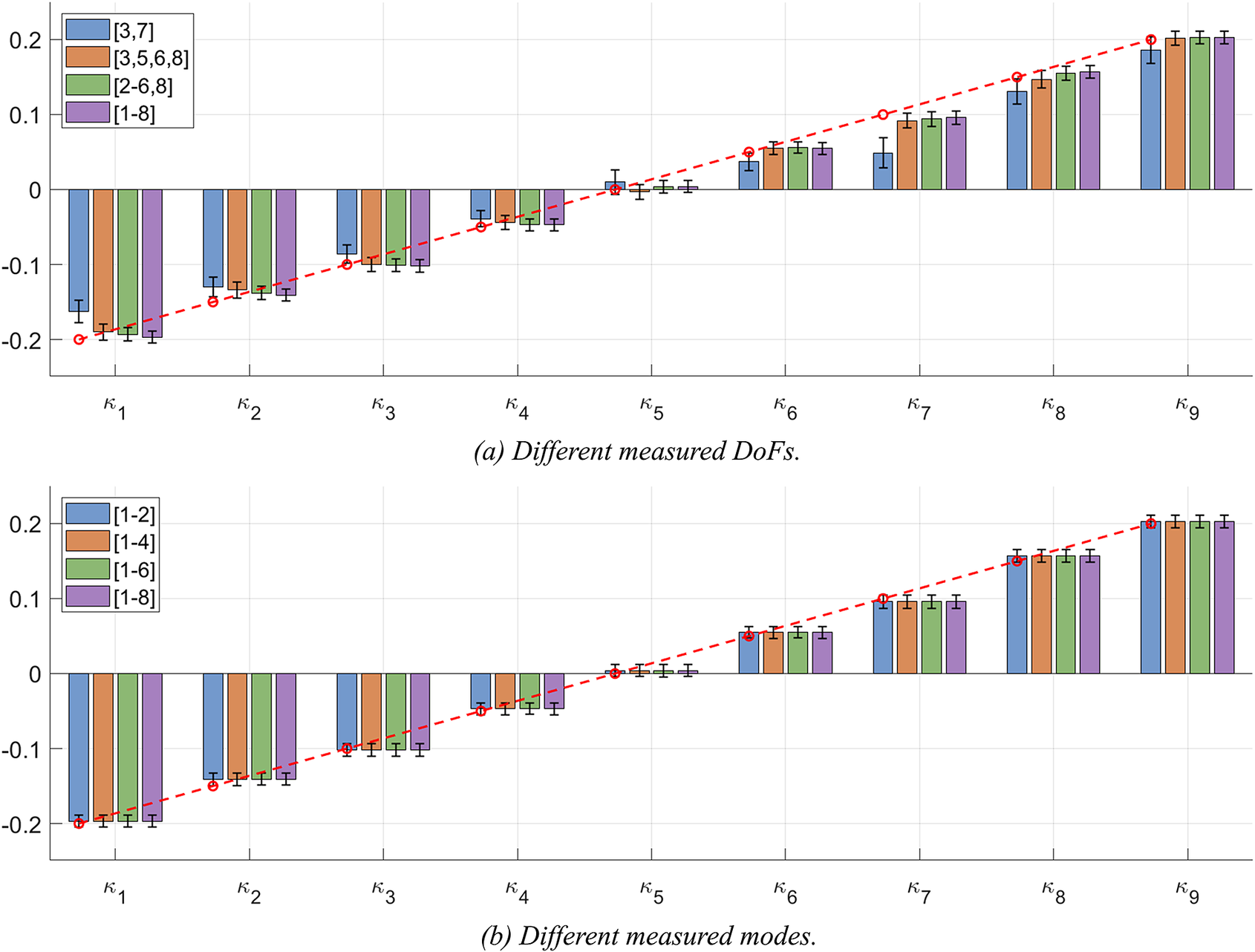

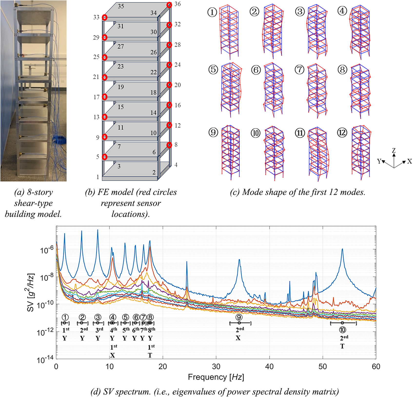
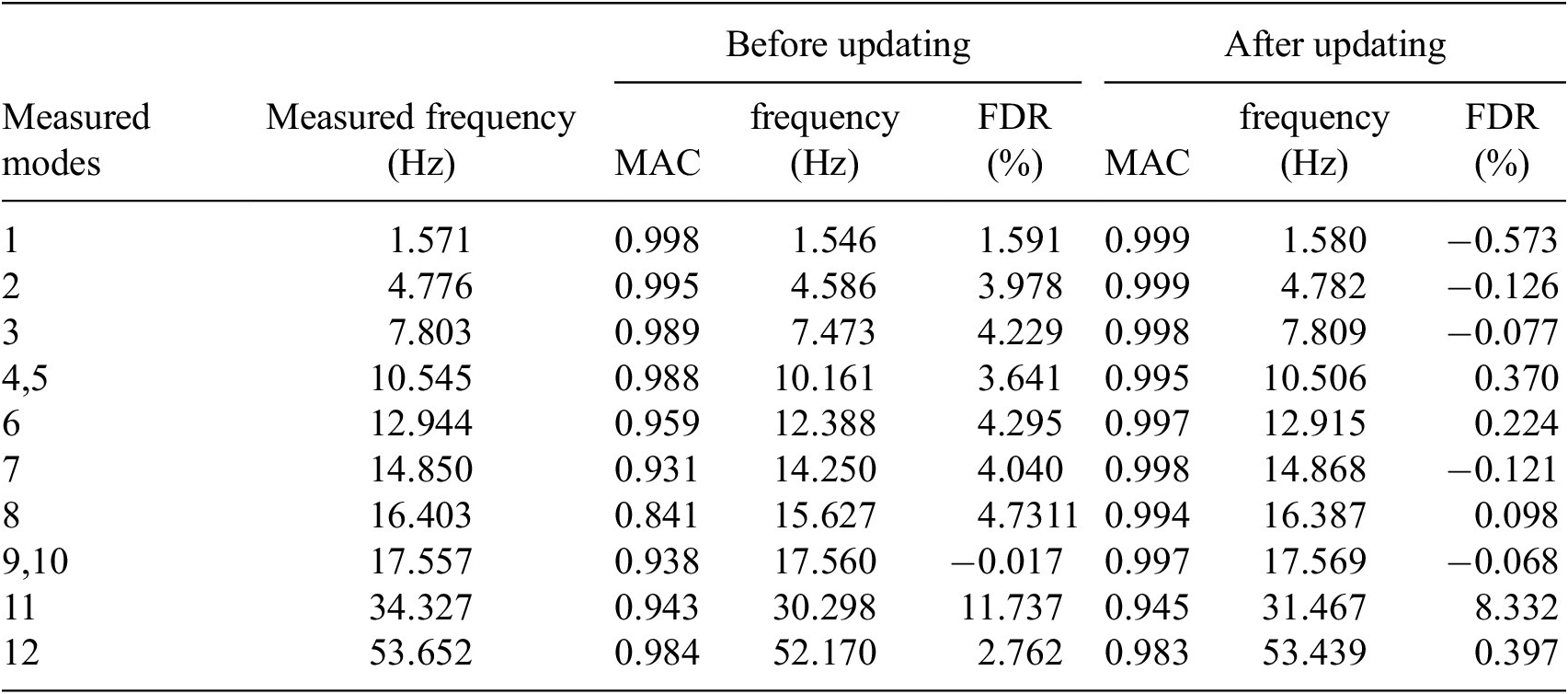
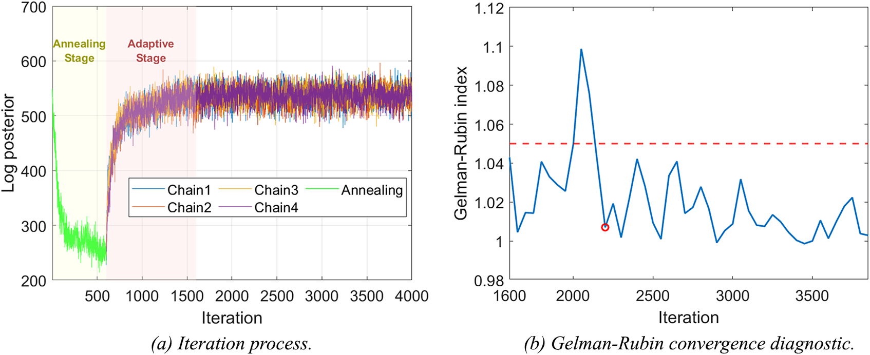
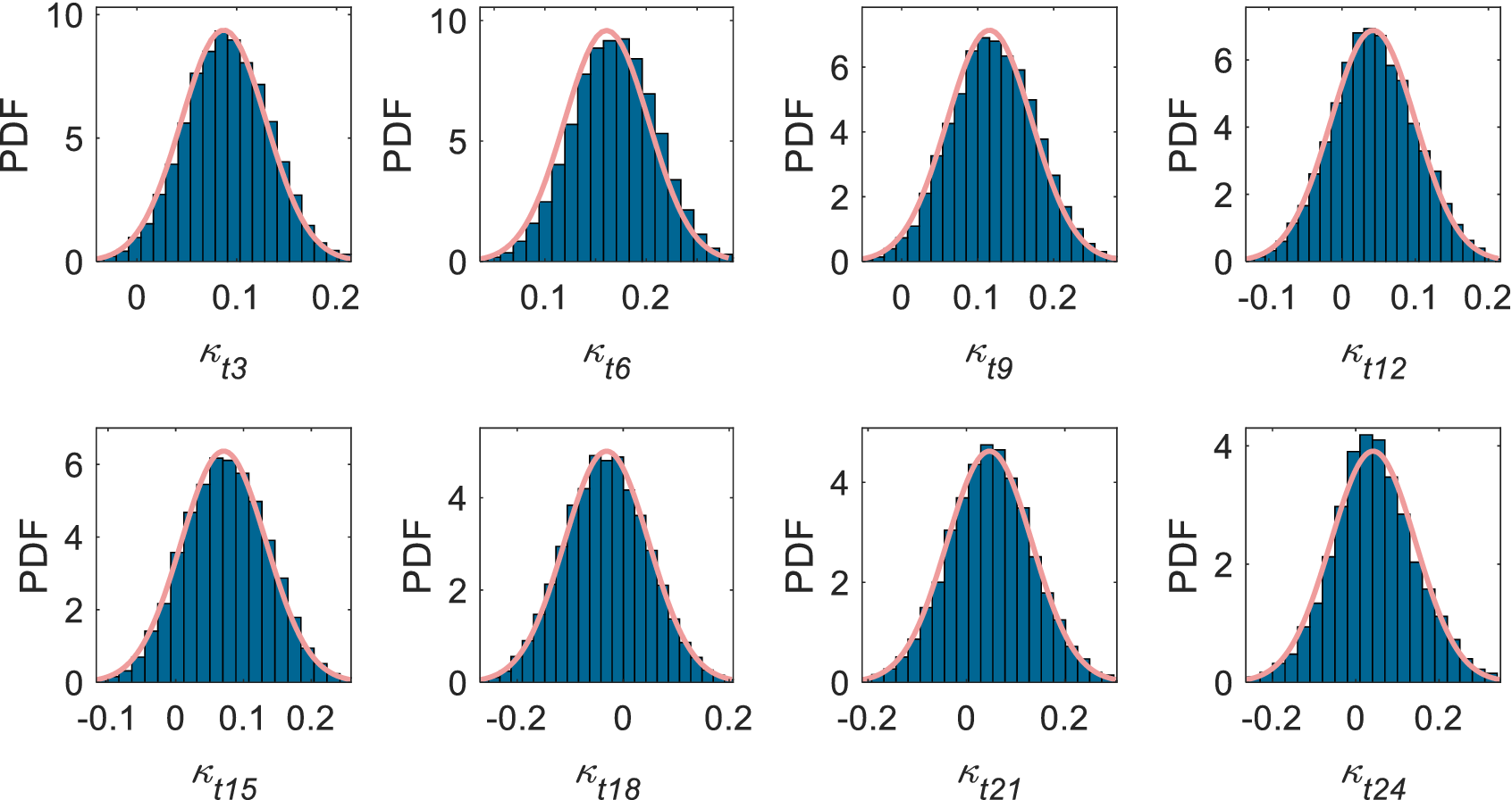

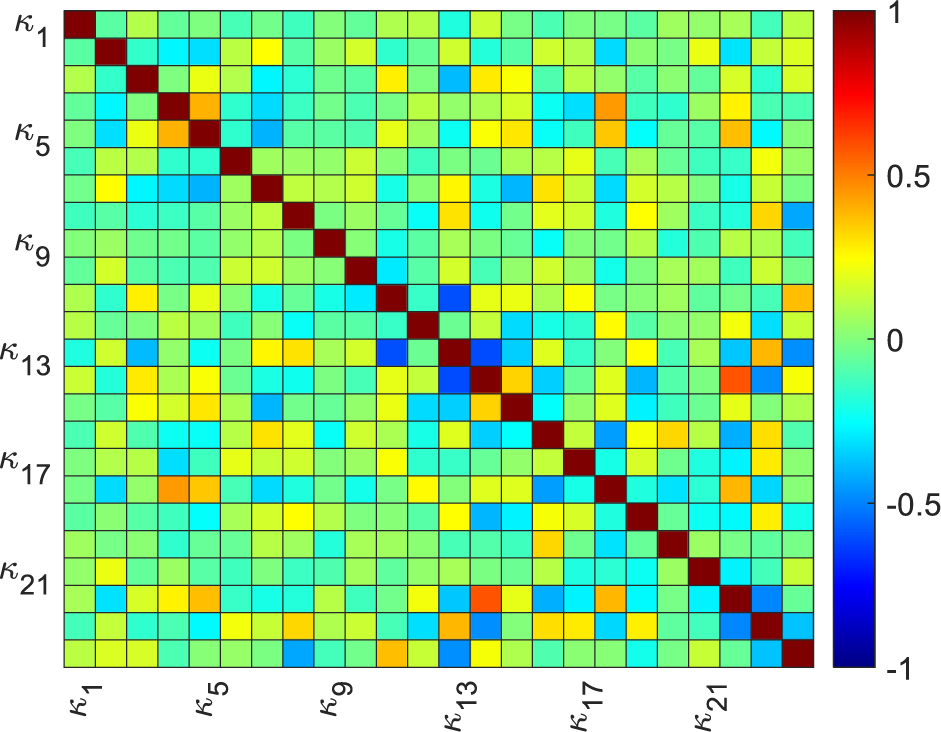
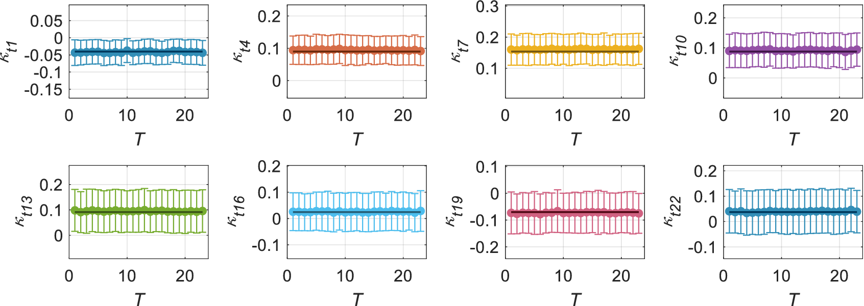


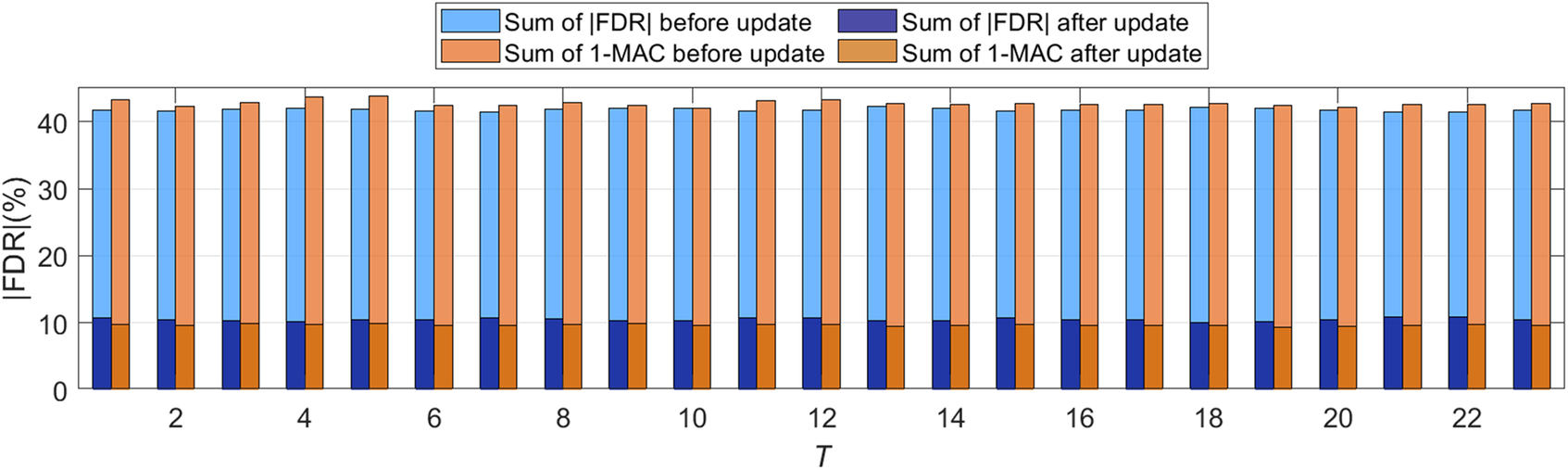
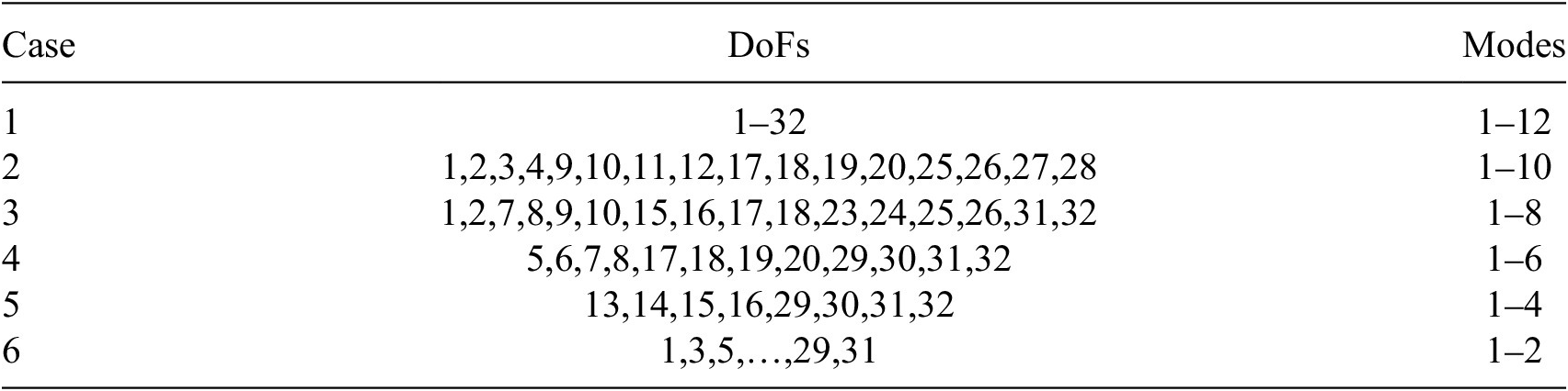
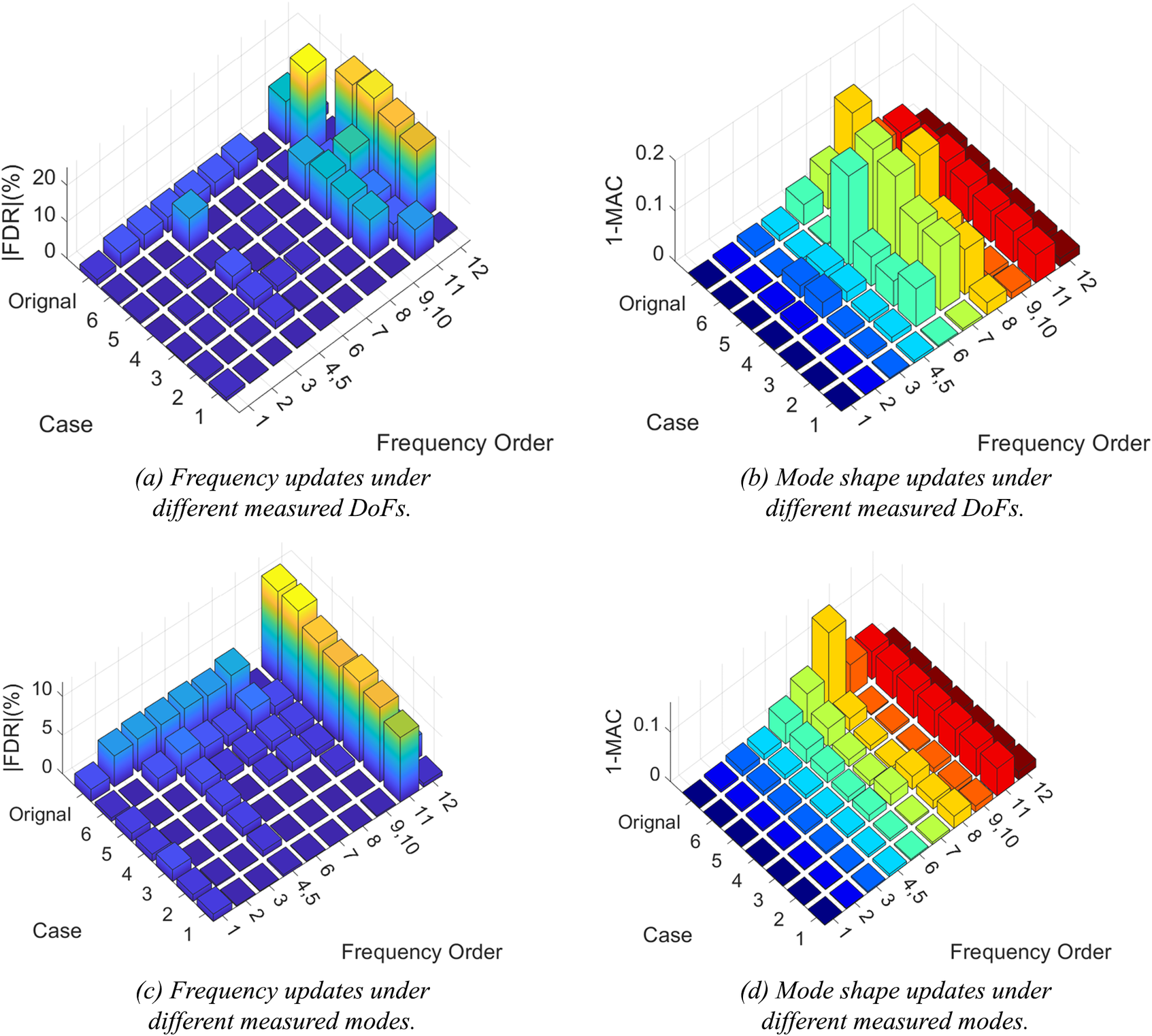
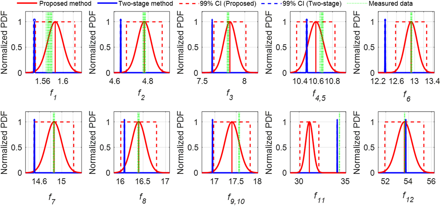
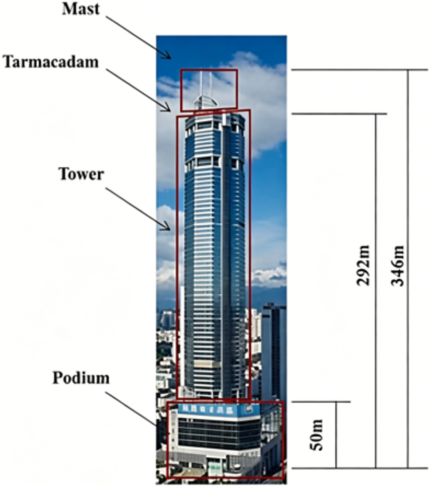
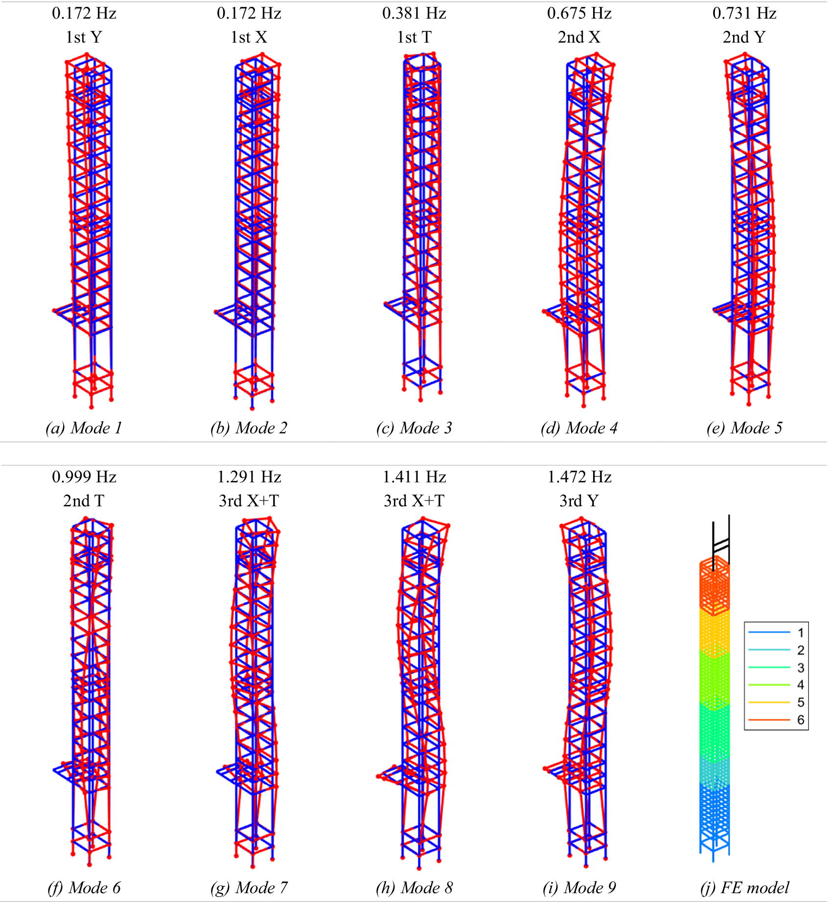
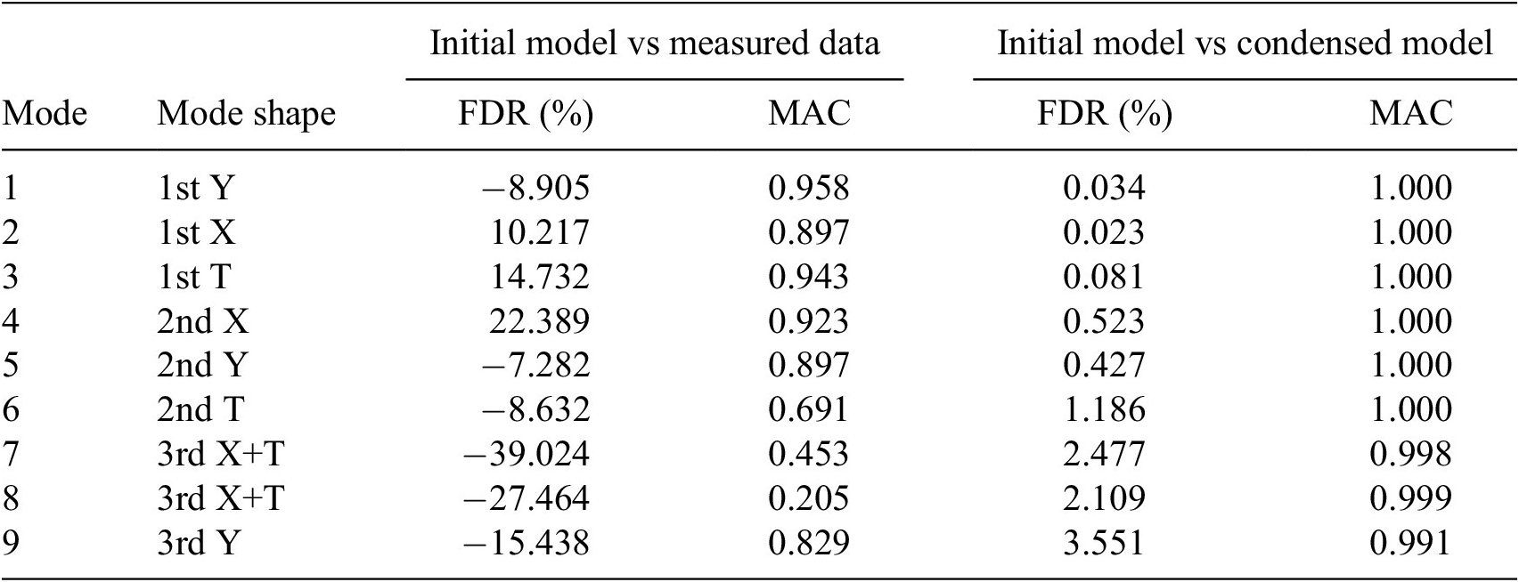
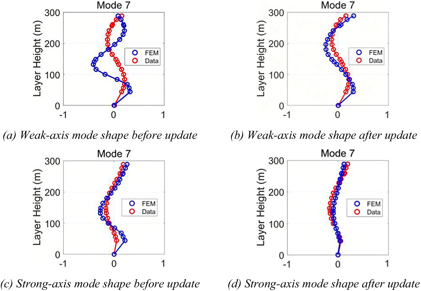
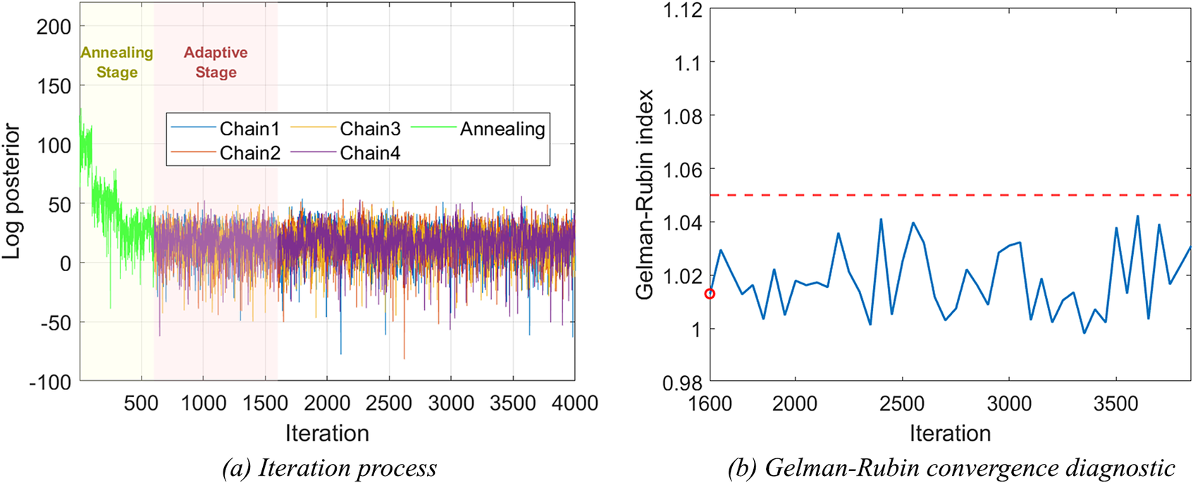
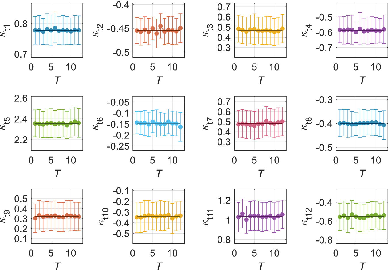


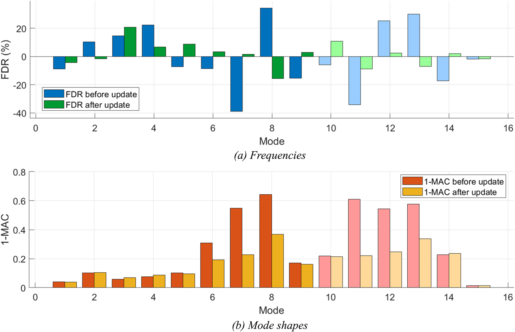
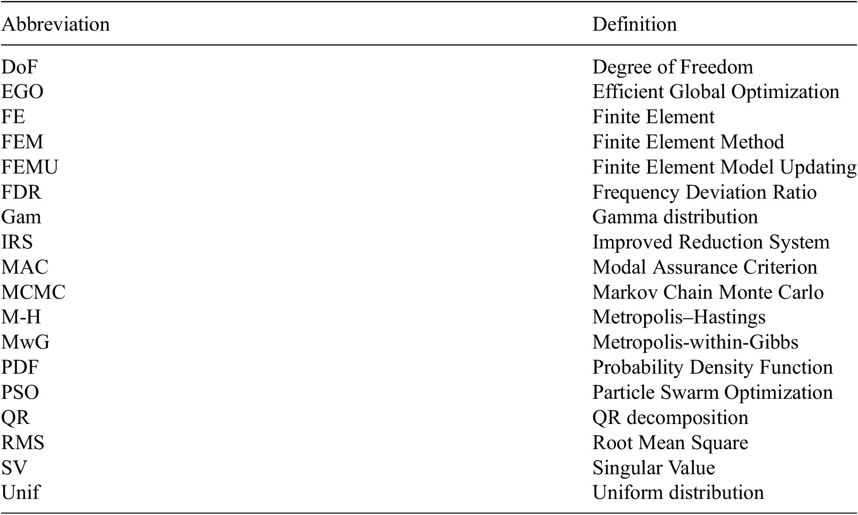

 Open access


Comments
No Comments have been published for this article.