

1. Introduction
A basic question about any ice sheet concerns whether or not it is thickening or thinning. One way to answer that question is to model the steady-state properties of the ice sheet and then compare the model with measurements. A common approach along this line infers the steady-state depth-averaged velocities from a model based on mass continuity. The continuity calculation is initiated with measurements of ice-sheet surface elevation, ice thickness, and surface and basal accumulation rate. The calculated velocities are known as balance velocities because they represent the ice-sheet depth-averaged speeds in the downslope direction that would result if the amount of snow added annually to a volume of the ice sheet equaled the amount of mass lost from that volume through advection or melting (Reference Budd, Jenssen and RadokBudd and others, 1971). If the surface balance velocities inferred from the (depth-averaged) balance velocities are higher than the measured velocities, the ice sheet is thickening and vice versa.
In this paper, we present computed surface balance velocities and error budgets for the Antarctic ice sheet. Our analysis builds on previous research (Reference Budd, Jenssen and RadokBudd and others, 1971, 1982; Reference Budd and SmithBudd and Smith, 1985; Reference Budd and WarnerBudd and Warner, 1996; Reference Bamber, Hardy and JoughinBamber and others, 2000a, Reference Bamber, Vaughan and Joughinb; Reference Huybrechts, Steinhage, Wilhelms and BamberHuybrechts and others, 2000) by adapting and modifying an algorithmic approach developed in the hydrology community (Reference Costa-Cabral and BurgesCosta-Cabral and Burges, 1994). Our numerical approach, which casts the outflow from a gridcell into a downstream flux matrix, refines the balance-velocity calculation by incorporating vector data on flow direction from the RADARSAT Antarctic Mapping Project (RAMP) image mosaic (Reference JezekJezek, 1999). The numerical implementation of our algorithm allows us to calculate a total error budget that includes errors arising from the input data and suggests how our algorithm may bias the final result. We validate our computed surface balance velocities and velocity errors through comparison with measured velocities on profiles encompassing Lambert Glacier and across ice streams draining into the Filchner Ice Shelf.
2. Balance-Velocity Equation
The mathematical expression of balance velocity for continuous fields is given by Reference Budd and WarnerBudd and Warner (1996), who also discuss approaches for discretizing the model. On a regular grid, the total flux from any gridcell is treated as a scalar with a fractional part of the flux going in orthogonal grid directions x and y. The portion of the flux in the x direction,|F x |, is related to an equivalent balance-velocity component |V x | as:
where H is the ice thickness, W is the square-grid cell-size dimension, |V| is the magnitude of the balance-velocity vector and θ is the flow direction with respect to the x axis. Similarly:
and the total flux |F| for a cell is:
Equations (1), (2) and (3) yield:
For comparison with measured surface data, Equation (4) is modified by the ratio r between balance velocity and the ice surface balance velocity |V S|, which takes into account the fact that the velocity decreases from the surface towards the bed. The value of r ranges from 0.8 to 1.0 (Reference PatersonPaterson, 1994) and we choose 0.9. |V S| then becomes
The value of r depends on properties such as ice temperature and basal conditions, so r will vary across the ice sheet. We select a constant value reflecting our lack of knowledge about spatial variability in r.
3. Numerical Evaluation of Balance Velocity
Several approaches for evaluating balance velocities start by determining the positions of flowlines. Balance velocities are calculated either by integrating fluxes over areas bounded by flowlines (Reference Budd, Jenssen and RadokBudd and others, 1971; Reference Joughin, Fahnestock, Ekholm and KwokJoughin and others, 1997) or by integrating point measurements along a flowline (Reference Radok, Barry, Jenssen, Keen, Kiladis and McInnesRadok and others, 1982). Although the technique accurately captures balance-velocity physics, flowline determination over long distances is prone to small errors in the surface slope and can be sensitive to the order (upstream vs downstream) in which flowlines are evaluated (Reference Radok, Barry, Jenssen, Keen, Kiladis and McInnesRadok and others, 1982). Most recent automatic approaches seem to over-concentrate flux towards the center of convergent flow (Reference Bamber, Hardy and JoughinBamber and others, 2000a).
Reference Budd and SmithBudd and Smith (1985) devised an automatic gridded technique that does not rely on an initial estimate of flowline positions. Reference Budd and WarnerBudd and Warner (1996) and Reference Fricker, Warner and AllisonFricker and others (2000) provide quantitative descriptions of a flowline-independent gridding technique that includes four generic steps: digital elevation model (DEM) preparation; flow-direction estimation; flux estimation; and final balance-velocity estimation. The first and last steps are common between different investigators (Reference Budd and WarnerBudd and Warner, 1996; Reference Bamber, Hardy and JoughinBamber and others, 2000a, b) and we essentially adopt a similar approach, as discussed below. There are different options for the second and third steps in which we have made modifications to procedures for estimating flow direction and flux. We discuss these below in comparison with the work of other investigators.
3.1. DEM preparation
We use the 1 km DEM from Reference Liu, Jezek and LiLiu and others (1999) in Arc/ Info grid format. We filter the DEM using a running, locally adaptive, Gaussian weighting window corresponding to an averaging dimension of 20 times the ice thickness (Reference PatersonPaterson, 1994; Reference Bamber, Hardy and JoughinBamber and others, 2000a). At the margin of Antarctica, the DEM is smoothed to the local mean to avoid edge effects.
Residual sinks (that is a local depression from the mean slope, resulting from data measurement error or data rounding) are filled using the Arc/Info grid function. The function raises the elevation of the sink to match the lowest height of the eight neighboring cells.
The filtered DEM is bilinearly resampled into a 20 km cell-size grid, which corresponds to the cell size used by Reference Budd and WarnerBudd and Warner (1996). The bilinear interpolation function provided by Arc/Info 8.1 assigns the value for an output cell using the weighted average of the four closest input cell centers to the output cell center. Ice-flow directions are determined from terrain slopes calculated from the 20 km data.
3.2. Flow direction estimation
Flow direction is calculated by estimating the direction of steepest slope using a DEM. Reference Budd and WarnerBudd and Warner (1996) calculate the slope components α x and α y for cell c i,j having elevation E i,j using the elevations of four cardinal nearest- neighbors surface elevations E i_1,j , E i,j+1 E i+1,j and E i,j-1, where subscripts i and j represent the row and column indices, respectively, of the DEM grid:
where W is the gridcell dimension. The flow direction θ is given by
where α is the magnitude of the slope.
We use the Reference Costa-Cabral and BurgesCosta-Cabral and Burges (1994) fitting plane algorithm to derive flow direction from the DEM. The algorithm uses the four most widely separated cell (diagonal cells about the evaluation cell) heights, E i-1,j-1, E i-1;j+1, E i+1,j-1 and E i+i,j+1, to fit a plane. The algorithm assigns the facing direction of the plane to the flow direction. The slope components (α x ,α y ) for cell c i,j are:
The flow directions θ is given by
The flow direction in either low-slope (Reference Lea, Parsons and AbrahamsLea, 1992; Reference Liang and MackayLiang and Machay, 1997, 2000; Reference TarbotonTarboton, 1997) or highly convergent regimes are unreliable. To mitigate this problem, we incorporate flow-direction information from imagery. In regions where the ice has been, or at least is assumed to be, in equilibrium, available information on flow stripes from the RAMP imagery is taken to accurately reflect the flow direction (Reference JezekJezek, 1999). Our approach is to use the two endpoints of each segment in the flow-stripe-vector dataset to calculate the flow direction for that segment. We then convert the flow-stripe-vector data into grid data, giving the gridcell value the flow direction of the closest line segment to the cell center if the line segment is within the cell. We merge the flow-stripe directions with surface-slope-derived flow directions by preferentially selecting the flow-stripe orientation. Incorporation of vector data mitigates the sensitivity of flow direction to DEM errors in low-slope areas and, to some extent, regions of converging flow. Flow stripes can incorrectly bias the result if the flow field has evolved over time. This is probably a greater problem on ice shelves, which are not treated in this analysis.
3.3. Flux and velocity estimation
Given estimates of flow direction and mass discharge per cell, partition schemes are used to model how much mass flows from one cell into one or two neighboring cells. Reference Budd and WarnerBudd and Warner (1996) partition the mass into downstream cells by multiplying the total scalar flux out of a gridcell by terms defined as
where x and y refer to the orthogonal grid directions.
As noted by Reference Budd and WarnerBudd and Warner (1996), the actual choice of partitioning scheme has little effect on the calculation (though as noted later the choice can play a role in the error model).
We favor the Reference Costa-Cabral and BurgesCosta-Cabral and Burges (1994) partition scheme wherein partitioning is proportional to areas defined by segmenting the cell into two regions separated by the flow-direction vector. The partitioning using the Reference Costa-Cabral and BurgesCosta-Cabral and Burges (1994) approach goes as:
where the definition of θ is slightly modified so that 0° ≤ θ ≤ 45°: now, we essentially define θ as the angle of the balance-velocity vector with respect to the cardinal direction (x or y), whichever is closer to the balance-velocity direction.
Partition schemes model how one cell discharges mass into neighboring cells. The next step is to form the drainage system using a flux algorithm model describing the contributions from all the cells. Reference Budd and WarnerBudd and Warner (1996) begin by sorting the DEM in descending order of elevation. Their algorithm depends on DEM sorting order, which makes it sensitive to DEM error.
In another approach that builds on the idea of using flow bands to calculate flux, Reference Costa-Cabral and BurgesCastal-Cabral and Burges (1994) trace upslope the flowlines passing through cells which then define the boundaries of contributing areas. Because the algorithm relies on flow directions to define contributing areas, flow-direction errors at the early stage of the calculation can create large errors in contributing areas.
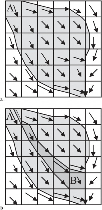
In a related approach, Reference Costa-Cabral and BurgesCosta-Cabral and Burges (1994) treat each cell as an initial condition wherein the flux entering the cell is simply the surface accumulation rate (advected fluxes are not included in the flux of the cell chosen for the start of the calculation). The discharge flux from the initial cell is allowed to flow downslope as an advective term until it encounters cells that are sinks or leaves the terrain. Once the discharge from every cell is calculated into a so-called influence matrix bounded laterally by flowlines, the total mass passing through each cell is summed (both accumulation and advection terms). In this way, the total mass passing through a particular cell equals the total mass drained by every upstream cell.
Figure 1a illustrates the influence-matrix idea. The gray region is the influence matrix of cell A. Every cell in the gray region receives some amount of advected mass from cell A. The boundaries of the influence matrix are flowlines so that there is no diffusion of mass across the boundary. Figure 1b is an example of how the flux into cell B is determined by a subset of flowlines which bound the dark gray region of Figure 1b. Though the influence matrix determined by flowlines is conceptually very accurate, it is hard to write an efficient and accurate computer program.
(a) The influence matrix associated with cell A where every gray cell receives some amount of mass from cell A. (b) The amount of mass received by cell B is determined by the careful downslope tracing of flowlines as described in the original Reference Costa-Cabral and BurgesCosta-Cabral and Burges (1994) approach. The accuracy of the estimated flux to cell B is strongly influenced by the accuracy of the derived flowlines that bound the dark gray region in (b).
We modify the downslope algorithm (Reference Costa-Cabral and BurgesCosta-Cabral and Burges, 1994) by focusing on the influence-matrix aspect of their model but abandoning explicit calculation of flowlines. This allows for a tractable code while retaining the advantage that it does not depend on DEM sorting order. As noted later, this modification does result in artificial mass diffusion through the grid.
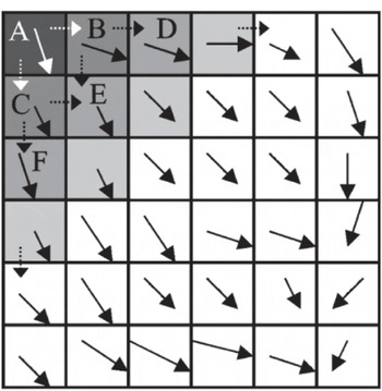
The influence matrix represents the flux distribution for a cell using only the accumulated mass at that cell as a flux source. Hence every cell is associated with a downstream influence matrix. The algorithm calculates the influence matrix for every cell and sums up influence matrices to obtain the total flux distribution. The algorithm builds an influence matrix cell by cell by successively partitioning mass from one cell into its downslope cells according to the partitioning scheme proposed by Reference Costa-Cabral and BurgesCosta-Cabral and Burges (1994). Partitioning proceeds until the edge of the terrain is reached. In Figure 2, flux from the originating cell A is partitioned into B and C and so on. The cells with the same gray tones are processed at the same time. We call these cells the frontline, and some care has to be taken when complex terrain may cause subsequent backflow into these cells (note that this problem is avoided in DEM sorting methods). Both the influence-matrix and DEM sorting techniques suffer from diffusion, by which we mean the artificial distribution of mass away from boundaries that would properly be identified as flowlines (Reference TarbotonTarboton, 1997).
Modified DEMON-Downslope algorithm (influence-matrix algorithm).
Since the influence-matrix algorithm does not use the DEM order to process cells, it is initially less affected by the DEM errors in flat or near-flat areas. The influence-matrix approach also yields a picture of the upslope areas contributing to a cell and the downslope areas fed by a cell. This aids in visualizing the flux calculation and helps validate the flux calculation.
To describe the influence-matrix algorithm, we need a notation that discriminates between a cell assigned to be the origin of an influence matrix from the same cell when it is used as a point for summing the flux from all upstream influence matrices. When a cell (or related property) is regarded as the start of an influence matrix, we use superscripts. When the cell is regarded as a receiving cell of flux from upstream cells we use subscripts. The contribution of flux from originating cell cl’m arriving at cell c i,j is then
where Sl,m
is the cell area and ![]() is the accumulation rate of matrix-origination cell c
l,m
, and λ0... λ
p
are the partition fractions using the Reference Costa-Cabral and BurgesCostal-Cabral and Burges (1994) partition scheme (Equation (11)).
is the accumulation rate of matrix-origination cell c
l,m
, and λ0... λ
p
are the partition fractions using the Reference Costa-Cabral and BurgesCostal-Cabral and Burges (1994) partition scheme (Equation (11)).
The total flux ![]() through cell c
i,j
is:
through cell c
i,j
is:
where the sums are taken over the cells that have influence matrices that include cell c i,j .
Once fluxes for every cell have been calculated, the balance velocity is computed according to Equation (5).
3.4. Error estimation
Uncertainty in the balance velocity comes from measurement errors associated with the observations and from the behavior of the algorithms. Errors in the behavior of the algorithm can be subtle and they also bias the way we estimate random errors. Here, we begin by discussing the effect of random errors in the observations on the balance velocity. We go on to discuss how artificial mass diffusion associated with the algorithm also causes errors in the final results.
Random errors in the DEM, accumulation rate and ice thickness are estimated from the data-source documentation. These errors propagate when the associated data are used to calculate flow direction, flux and balance velocity. We apply the maximum error propagation theory to estimate the error from input data. Essentially if y = f (x 1,x 2,..., x m ), and if the maximum errors for x 1,x 2,..., x m are δ x 1, δx 2,...,δx m , then the maximum absolute error Δy for y is:
The maximum absolute error of flow direction Δθ is from Equations (8) and (9):
where Δz is the absolute error in relative elevation between neighboring cell elevations. The absolute error of ![]() is:
is:
We estimate a maximum error of the last term to be:
Similarly, the absolute error Δλ of the partition function λ (Equations (11)) is:
Combining Equations (17) and (18) yields:
The relative error of ![]() is:
is:
![]() includes two characteristic parts. The first is error propagated from observation error in the accumulation rate. The second part includes DEM errors that propagate into computed surface slopes and hence the partitioning factors λ. The error associated with the partitioning scheme and the flux estimation algorithm propagates through the influence matrix via the terms:
includes two characteristic parts. The first is error propagated from observation error in the accumulation rate. The second part includes DEM errors that propagate into computed surface slopes and hence the partitioning factors λ. The error associated with the partitioning scheme and the flux estimation algorithm propagates through the influence matrix via the terms:
In that sense, Equation (21) implicitly includes diffusion effects, which serve to increase the error estimate at each gridcell.
The error Equations (16–19) also show how errors are accumulated downstream from the ice divide. For a downstream cell, the flux error will increase as l and m increase (Equation (16)); in other words, error increases as the contributing area increases, or if a smaller gridcell size is chosen for the same area. Equation (19) also shows that when θ (the 0–45° angle between flow direction and cardinal direction) is close to 45°, ![]() is larger than when θ is close to 0°. Restated, the smaller the angle between flow direction and cardinal direction, the less the diffusion. Note that partitioning using Equations (10) would yield a minimum error at 45° to the grid direction, which we believe is less desirable because the algorithm only allows for flow orthogonal to the grid direction.
is larger than when θ is close to 0°. Restated, the smaller the angle between flow direction and cardinal direction, the less the diffusion. Note that partitioning using Equations (10) would yield a minimum error at 45° to the grid direction, which we believe is less desirable because the algorithm only allows for flow orthogonal to the grid direction.
We use these results to estimate balance-velocity errors. By Equation (5), the absolute error of surface balance velocity, ΔV S, is:
The fractional error is:
We note again that we assign a constant value (0.9) for the ratio between depth-averaged mean velocity and the surface velocity (Equation (5)). Given the range of probable values for r, we assign the error on r to be 0.1.
4. Datasets
We used four primary datasets in this analysis: the OSU (Ohio State University) DEM of Antarctica (Reference Liu, Jezek and LiLiu and others, 1999); the BEDMAP ice-thickness model (Reference Lythe and VaughanLythe and others, 2000); surface accumulation rates (Reference Vaughan, Bamber, Giovinetto, Russell and CooperVaughan and others, 1999); and RAMP flow stripes (Reference JezekJezek, 1999).
The elevation data contained in the DEM from Reference Liu, Jezek and LiLiu and others (1999) are from several topographic datasets that have rather disparate sampling intervals. Consequently, the interpolated product was uniformly resampled to 200, 400 and 1000 m post-spacings recognizing that in some areas this represents an over-sampling of the available data. Similarly the quality and accuracy of the data varies due to data collection methods as discussed in Reference Liu, Jezek and LiLiu and others (1999). For error analysis purposes, we are only concerned with the absolute error in relative elevation z between adjacent observations: we take Δz in Equation (15) to be 1 m.
Reference Vaughan, Bamber, Giovinetto, Russell and CooperVaughan and others (1999) summarize accumulation rate data. Their product is available as a 10 km cell size, Arc/Info grid. It is assembled from over 1800 published or unpublished in situ measurements. The uncertainty of the data is approximately 10%.
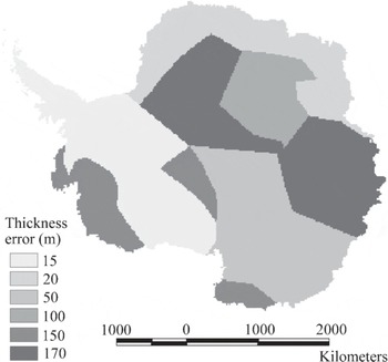
Ice thickness was compiled as part of the BEDMAP project (Reference Lythe and VaughanLythe and others, 2000). The data are provided in an Arc/Info grid with 5 km cell size. It is based on about 2 × 10⁶ ice-thickness observations by 12 countries over the last five decades. The accuracy of ice thickness is different in different regions and ranges from 10 to 180 m (Reference Lythe and VaughanLythe and others, 2000). A few areas, such as the Amery Ice Shelf, Filchner – Ronne Ice Shelf and West Antarctic ice streams, have good accuracy and excellent coverage (Reference Lythe and VaughanLythe and others, 2000). Other areas, such as large parts of East Antarctica, are covered by 50 km spaced flight-lines or with little to no data at all (there, ice thickness is based on gross interpolation or model results) (Reference Lythe and VaughanLythe and others, 2000). We estimated ice-thickness errors according to known properties of the data collection methods (Fig. 3).
Estimated error in ice thickness.
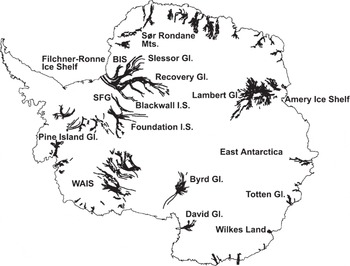
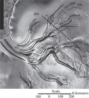
Flow stripes in the fast ice streams and ice shelves are evident on the 1997 RAMP imagery. As part of a separate project, the stripes were manually digitized and then converted into Arc/Info line coverage. Long, linear features were judged to be flow stripes based on continuity, correlation with known glaciologic features (e.g. ice streams) and general directions relative to a priori knowledge of surface topography (e.g. features running orthogonal to the generally known topography were not identified). Figure 4 shows the digitized flow-stripe map from the RADARSAT mosaic. Of these, we used in this analysis the flow stripes drawn for: the ice streams draining into the Filchner–Ronne and Ross Ice Shelves; the Lambert drainage system; Byrd, David and Pine Island Glaciers; and outlet glaciers through the Sør Rondane Mountains. We incorporate the flowline information into the analysis by determining the x-y coordinate of each node making up the line. The line coverage is converted into a line segment coverage, and the nodal coordinates of the ends of each segment are used to compute the orientation that is saved as an attribute of each segment. The line segment coverage is then gridded into a 20 km cell where the values of the cell are the orientation angles of the line segments nearest to the center of the cell. The last step is manual inspection and editing (Reference WuWu, 2002).
Digitized flow strips and place names referred to in the text. Abbreviated names are: BIS, Bailey Ice Stream; SFG, Support Force Glacier; WAIS, West Antarctic ice streams.
5. Results
Surface balance velocities calculated using the algorithm described in section 3 are shown in Figure 5 on a 20 km grid. Velocities are not calculated over the ice shelves because the flow directions both from the DEM and from flow stripes are suspect. We have created an ice-shelf mask and applied it to all of our maps. The mask is based on a coastline derived from the RAMP mosaic (Reference Liu and JezekLiu and Jezek, 2004) and Antarctic Digital Database (ADD Consortium, 2000) grounding-line data. As noted by Bamber and others (2000b), the surface balance-velocity distribution map shows complexities in flow from the ice divides to the coast. Channeled flow is evident around the entire continent and through major outlet glaciers such as David Glacier in northern Victoria Land. The map captures the network of tributaries that feed the West Antarctic ice streams draining into the Ross and Ronne Ice Shelves. The similarly complex flow of the ice streams draining into the Filchner Ice Shelfis also evident. In particular, the surface balance-velocity map depicts the flow of the newly discovered Blackwall Glacier (Reference JezekJezek, 1999; Reference Gray, Short, Mattar and JezekGray and others, 2001). Blackwall’s twin, RAMP Glacier, is absent from the balance-velocity map even though it appears more clearly in the RADARSAT mosaic (Reference JezekJezek, 1999). We suspect that the glacier is missed in our model because of the sparse ice-thickness data available for this region. Organized flows associated with Recovery Glacier and Support Force Glacier and Foundation Ice Stream snake hundreds of kilometers into East Antarctica. Flow associated with Support Force Glacier and Foundation Ice Stream extends nearly to the divide, which partitions flow to the Filchner and Ross Ice Shelves. Just on the opposite side of the divide, tendrils of organized flow descend into Byrd Glacier. Some of the least complex flow appears in Dronning Maud Land where a broad lobe of slow-moving ice extends towards the coast before the coastal mountains bifurcate the flow into several smaller glaciers.
Surface balance-velocity map (Vs).
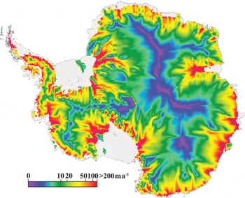
Figure 6 shows our estimates of surface balance-velocity errors from Equation (22). As might be expected, errors on the interior ice sheet are a few tens of meters per year where flow is relatively simple and errors are primarily due to local uncertainties in ice thickness, accumulation rate, surface slope and the velocity ratio r. As flow is channeled, errors begin to grow and can exceed several hundred m a-1 at the mouths of outlet glaciers and ice streams.
Surface balance-velocity error estimate (ΔV s)
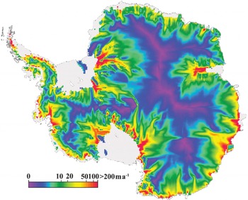
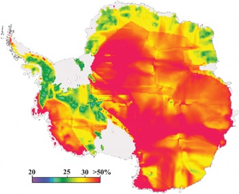
Figure 7 is the percentage error in surface balance velocity. The blockiness in Figure 7 is caused by the regional assignments of errors in ice thickness. Percentage errors are less than about 40% over much of the ice sheet where the primary contributors to error are local accumulation rate, ice thickness and velocity ratio r uncertainties. Errors are largest in regions of converging flow and where the flow approaches an angle of about 45° to the cardinal direction.
Percentage errors in balance velocity (ΔV s/V s)
6. Validation and Discussion
We compare the surface balance-velocity result with independently measured velocity to validate our calculation. We also compare our influence matrix approach to our implementation of the DEM sorting algorithm. Our sorting algorithm calculates flux from the highest to lowest elevation cell, partitioning the flux between cells using Equations (11). The direction angle for flux partitioning from each cell is based on the flow-stripe direction (where available) rather than the direction from the DEM slope. This is a modification to the DEM sorting approach described by Reference Budd and WarnerBudd and Warner (1996). By including the flow-stripe information in the algorithm, we introduce an inconsistency in that the DEM is assumed accurate for elevation sorting. By changing the flow direction from slope to flow stripes, we are implying that there are DEM errors that in turn imply that the sort order may be wrong. For the influence-matrix approach, we start with the DEM and calculate flow directions. We then essentially discard the DEM elevation data. We finally make modifications to the flow field using the flow stripes. We think this is a physically more consistent approach.
6.1. Lambert Glacier
Global positioning system (GPS)-derived velocities were collected along a profile around the Lambert Glacier drainage system as part of the Australian National Antarctic Research Expedition (Fig. 8). The velocities are available through the U.S. National Snow and Ice Data Center website (http://nsidc.org/data/velmap/amery/amery.html) and we compare these to our balance-velocity results.
Lambert Glacier and Amery Ice Shelf. Repeat GPS velocity measurement sites are shown by the black dots. Flowlines are based on interpretation of the RADARSAT mosaic.

Surface balance velocities are resampled for comparison with the GPS-derived velocity data VGps, using the nearest gridcell interpolation method from the original 20 km cell- size surface balance-velocity result. The results are compared in Figure 9 and Table 1. The mean difference between the influence-matrix model Vs_in and the measured result is 2.1 m a-1 with standard deviation of 9.2 m a-1. The mean difference between balance velocity using the DEM sorting algorithm, Vs_ds, and VGps is 2.5 m a-1 with standard deviation of 9.7 m a-1. The mean difference between balance velocity using the influence-matrix algorithm without using flow stripes to correct flow directions, VS_no, and VGps is 2.7 m a-1 with standard deviation of 10.5 m a 1. In this case, all the approaches perform about equally, presumably because the DEM (and hence the derived flow directions) as well as the other observational data are accurate in this well-studied region. If the DEM was inaccurate, we might expect an improved result when flow-stripe information was added to the mix.
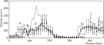
Measured (solid line) and calculated (black squares) velocity profiles around Lambert Glacier. Errors in measured velocities are < 1 m a -1.
Surface balance velocity comparisons with GPS velocity (VGps) for the Lambert Glacier drainage area
As illustrated in Figure 9, the VS_in estimates generally agree with the VGps data to within the calculation errors. Model and measurements deviate somewhat at locations A, B and C–D. The lateral scales of the anomalies at A and B are only one or two gridcells and we suspect our model simply does not have the resolution to capture these features. Anomalies between C and D are large in lateral scale (relative to the grid size) and in the overall negative difference between measured and modeled velocities (relative to the estimated errors). Points C and D bound the flow of a central tributary feeding Lambert Glacier. The negative differences between measured and modeled velocities suggest that this area is thickening. Previous to our analysis, Reference Fricker, Warner and AllisonFricker and others (2000) compared measured and modeled balance fluxes for the Lambert drainage basin. They used a DEM sorting approach to model the flux computed on a 5 km grid. They conclude as we that the flow outside the band between about 800 and 1500 km in Figure 9 is in balance to within the accuracy of the calculation. Our result suggests that the stream region between 800 and 1500 km is also in balance save for the narrow zone bounding the central tributary of Lambert Glacier (C–D). We note, however, that our balance-velocity errors may be significantly underestimated if, as Reference Fricker, Warner and AllisonFricker and others (2000) suggest, the accumulation rate uncertainties greatly exceed our assigned value of 10%.
6.2. Ice streams draining into the Filchner Ice Shelf
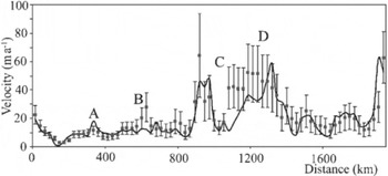
Reference ZhaoZhao (2001) used RADARSAT interferometric data to measure surface velocities of ice streams draining from East Antarctica into the Filchner Ice Shelf (Fig. 10). The resulting velocity fields were compiled into a 200 m cell grid with an estimated speed accuracy of 15 m a-1. We compared the InSAR velocities VInsAR to surface balance velocities calculated using the nearest-gridcell interpolation method applied to the original 20 km cell-size surface balance- velocity result. The dashed line in Figure 10 shows the profile location and Figure 11 shows the results. Note the improved agreement between surface balance velocities and measured velocities when flow-stripe information is used in the analysis. In Table 2, the mean difference between surface balance velocity using the influence-matrix algorithm VS_in and interferometric velocity VInsAR is 3.5 m a-1 with standard deviation of 48.9 m a-1. The mean difference between balance velocity using the DEM sorting algorithm Vs_ds and VInsAR is 10.0 m a-1 with standard deviation of 45.9 m a-1. The mean difference between InSAR velocities VinsAR and balance velocities Vs_no calculated using the influence-matrix algorithm but without using flow stripes to correct flow directions is13.8ma-1with standard deviation of 71.9 m a-1.
Ice streams draining into the Filchner Ice Shelf, and profile line used to compare balance velocities to InSAR velocities Abbreviated names are: FIS, Filchner Ice Shelf; BIS, Bailey Ice Stream; RG, Recovery Glacier; BW, Blackwall Ice Stream.
Measured (thick line) velocity and surface balance velocity profiles across ice streams draining into the Filchner Ice Shelf. Influence-matrix result with flow-stripe information is shown by the black squares. The short-dashed line shows the influence-matrix result without flow-stripe information. DEM sorting approach with flow-stripe information is shown with the long-dashed line.
Surface balance velocity comparisons with interferometry velocity (VinsAR.)
There is generally good agreement between the InSAR observations and the calculated balance velocities. Point A corresponds to the inferred margin of Bailey Ice Stream, which Reference ZhaoZhao (2001) reported to be thickening by 0.25 ± 0.06 m a-1. The increasing difference between balance velocities and InSAR velocities from the start of the profile to about 30 km past point A weakly supports Zhao’s observation. The peak flux from Slessor Glacier is located at point C and there is little significant difference between measured and modeled velocities, suggesting, as did Zhao, that Slessor Glacier is in equilibrium. The profile intercepts the northern margin of Recovery Glacier at point D. The balance velocities are statistically smaller than the measured velocities near the center of the ice stream, again weakly supporting Zhao’s calculation which indicates that Recovery Glacier is thinning by 0.23 ± 0.22 ma-1. However, we are cautious about drawing a firm conclusion about Recovery Glacier because of the very limited ice-thickness data available for this region.
As a further comparison, we have overlaid the measured flow stripes onto the balance-velocity map in Figure 12. As noted, most of the flow stripes are used in the balance- velocity calculation and in that sense the comparison serves as a consistency check. Shorter flow stripes associated with glaciers in Dronning Maud Land and Wilkes Land were not used in the calculation. Although the orientations of these stripes match well with the patterns of balance velocity, the balance-velocity data indicate organized flow further into the interior than would be suggested by the flow stripes, for example the flow from Totten Glacier and around Law Dome, the flow down Byrd Glacier and the flow from Support Force Glacier and Foundation Ice Stream.
Flow strips and balance-velocity map (gray image with relatively faster speeds shown lighter than the darker relatively slower speeds).
7. Conclusion
We have developed a modified surface balance-velocity estimation approach. Our matrix approach allows us to visualize upslope source and downslope outflow areas associated with individual cells, which helps to validate results. It also facilitates error estimation and can be used to illustrate how errors from source data and biases from the form of the algorithm introduce uncertainty into the result. Our approach flexibly incorporates refined flow directions derived from image data in low slope or complex slope. We find favorable comparison with independent velocity measurements around Lambert Glacier and ice streams draining into the Filchner Ice Shelf. The comparisons suggest that both glacial regimes are close to equilibrium within the estimated errors. The computer code version of our balance velocity model is available from X. Wu.
Acknowledgements
This research was supported by a grant from the U.S. NASA Pathfinder Program and Polar Oceans and Ice Sheet Program. We are grateful to two reviewers (T. Payne and an anonymous reviewer) and the scientific editor, J. Meyssonnier, for their considerable efforts on our behalf.


