


1. Introduction
The effects of fiscal policy on the economy are a topic of continuing disagreements among Keynesian and neoclassical economists, as well as policymakers. In contrast to monetary policy, the macroeconomic effects of fiscal policy are relatively more controversial. During the global financial crisis and the Covid-19 pandemic fiscal stimulus moved center stage. However, high inflation in the post-pandemic period raises questions about the impact of fiscal stimulus packages. The commonly used measure of fiscal policy effectiveness is the fiscal multiplier. It describes the effect of an exogenous change in a fiscal policy instrument, be it an unexpected government spending or tax change, on real GDP. The literature on empirical fiscal multipliers is extensive. Multipliers generally range in value from 0.6 to 2 for government spending and -5 to 0 for tax changes (Ramey, Reference Ramey2019, Table 1, p. 102, and Table 2, p.105, respectively). Multipliers may also depend on the state of the economy.
In regards to the identification of fiscal shocks in structural vector-autoregressive (SVAR) models, there are several common approaches in the empirical literature. The seminal study of Blanchard and Perotti (Reference Blanchard and Perotti2002), as well as further work by Perotti (Reference Perotti2004), rely on imposing contemporaneous restrictions on the structural coefficient matrices in an SVAR. Such restriction are based on externally calculated elasticities of government spending and taxes with respect to output and other variables included in the VAR.Footnote 1 More recently, several authors have relied on identification through sign restrictions with penalty function (Mountford and Uhlig, Reference Mountford and Uhlig2009), the use of narrative fiscal shocks derived from outside the SVAR (Ramey, Reference Ramey2011; Romer and Romer, Reference Romer and Romer2010), or on narrative shocks used as external fiscal and non-fiscal instruments in so-called proxy-SVARs (Mertens and Ravn, Reference Mertens and Ravn2014; Caldara and Kamps, Reference Caldara and Kamps2017; Angelini et al. Reference Angelini, Caggiano, Castelnuovo and Fanelli2023).
The crucial point for our study is that the values of contemporaneous fiscal elasticities play a critical role for the size of the multipliers in the SVAR literature. Mertens and Ravn (Reference Mertens and Ravn2014) use a proxy-SVAR with narratively identified unanticipated tax shocks. They compare result from such a proxy-SVAR to a standard SVAR with externally imposed elasticities as in Blanchard and Perotti (Reference Blanchard and Perotti2002). Mertens and Ravn (Reference Mertens and Ravn2014) show that the tax multiplier in standard SVARs can range from an absolute value near one (Blanchard and Perotti, Reference Blanchard and Perotti2002) to values of around two or three, depending on the size of the output elasticity of tax revenues. They argue that lower tax multiplier values in previous studies can be explained by an imposed output elasticity of tax revenue value that is contradicted by empirical evidence. Caldara and Kamps (Reference Caldara and Kamps2017) demonstrate that the differences in fiscal multiplier estimates in SVARs can be analytically accounted for by different assumptions for the systematic response of tax and spending policies to output. Different fiscal rules lead to different identification schemes and different empirical multipliers. They propose instead a proxy-SVAR that uses non-fiscal external instruments to directly identify and estimate the parameters of alternative fiscal rules, without imposing external elasticities. Furthermore, Angelini et al. (Reference Angelini, Caggiano, Castelnuovo and Fanelli2023) also use a proxy-SVAR and show the set of instruments used can crucially affect multiplier, as is the case for imposing or not imposing an orthogonality assumption between tax shocks and their factor productivity shock. Also, external instruments in proxy-SVARs may be weak (Stock and Watson, Reference Stock and Watson2018), or altogether not valid (Nguyen, Reference Nguyen2025).
Baumeister and Hamilton (Reference Baumeister and Hamilton2015, Reference Baumeister and Hamilton2018, Reference Baumeister and Hamilton2019) develop a new approach for identifying structural relationships in a VAR model. The identification of structural shocks requires prior information about underlying economic relationships that are external and supplementary to the VAR model itself. Their methodology employs Bayesian priors to account for a researcher’s uncertainty around imposed identifying assumptions. The traditional and most commonly used approaches to identifying structural shocks in SVARs are to impose zero restrictions on contemporaneous relationships among structural shocks, specific values for variables’ elasticities to shocks, and/or sign restrictions. Instead of imposing such identifying restrictions as if they were know with certainty, Baumeister and Hamilton (Reference Baumeister and Hamilton2015) propose to explicitly account for the degree of uncertainty surrounding a researcher’s prior information. As outlined in Baumeister and Hamilton (Reference Baumeister and Hamilton2019), their approach allows for imposing varying degrees of a priori uncertainty about identifying values imposed, as well as for setting sign restrictions. In addition, it can deal with structural instability by assigning different weights to observations from different time periods. So far, the methodology has been applied to quantify the impact of monetary policy shocks in the U.S. economy (Baumeister and Hamilton, Reference Baumeister and Hamilton2018) and to evaluate the elasticities on the U.S. oil and natural gas markets (Baumeister and Hamilton, Reference Baumeister and Hamilton2019; Rubaszek, et al. Reference Rubaszek, Szafranek and Uddin2021). To the best of our knowledge, this framework has not been exploited to broaden the understanding of U.S. fiscal policy and pin down precisely fiscal elasticities.
We contribute to the existing literature across several margins. First, our model specification produces sensible estimates that allow us to assess the effects of fiscal policy while controlling for monetary policy for the U.S. economy. We estimate the level of fiscal multipliers. Second, we provide estimates of posterior short-term elasticities by applying Baumeister and Hamilton’s methodology. Third, we present a number of robustness checks where we change the prior assumptions the lag length, and we include post-Covid-19 observations.
The rest of the paper is structured as follows. In Section 2 we briefly review the related literature. Section 3 presents the Bayesian econometric model. Section 4 is dedicated to the data and the empirical specification, along with the choice of specific prior distributions. Empirical results are discussed in Section 5 and their sensitivity to modifications in the baseline model is explored in Section 6. Finally, Section 7 concludes the analysis.
2. Literature review of closely related fiscal SVAR models
Blanchard and Perotti’s (2002) widely cited study forms the foundation for most subsequent empirical research on fiscal multipliers. In their approach fiscal shocks are identified by using institutional information about the tax and transfer systems to specify the automatic response of taxes and spending to economic activity and, then, by imposing externally calculated elasticities. Blanchard and Perotti (Reference Blanchard and Perotti2002) use a trivariate SVAR model: the logarithms of quarterly government spending, GDP, and taxes, all in real and per capita terms.Footnote 2 Their main findings are the following. Government spending increases cause output to increase, while tax increases cause output to decrease. Spending multipliers are close to one and they depend on different components of output, meaning that private consumption increases following a government spending increase, while private investment is crowded out to some degree.
Mountford and Uhlig (Reference Mountford and Uhlig2009) and Mertens and Ravn (Reference Mertens and Ravn2014) apply similar data as in Blanchard and Perotti (Reference Blanchard and Perotti2002) but use a different methodology. Mertens and Ravn (Reference Mertens and Ravn2014) use a proxy-SVAR with unanticipated narrative tax shocks as an external proxy (instrument variable) and they allow for measurement error in the narrative tax shocks. On the other hand, Mountford and Uhlig (Reference Mountford and Uhlig2009) set instead sign restrictions on VAR impulse responses to achieve identification. They use a so-called penalty function approach, that rewards large impulse responses in the right directions more than small responses and penalizes responses of the wrong sign. Their sample covers the period from 1955 to 2000 for U.S. data. Mountford and Uhlig (Reference Mountford and Uhlig2009) consider three scenarios: deficit-spending, deficit-financed tax cuts and a balanced budget spending expansion.Footnote 3 They find that deficit-financed tax cuts are the most effective among the three scenarios with the largest present value multiplier equal to five after five years. Mountford and Uhlig (Reference Mountford and Uhlig2009) also find that deficit spending weakly stimulates the economy, more precisely, it crowds out private investment but without interest rate increases and without real wage increases.
The two papers that are most closely related to ours are Caldara and Kamps (Reference Caldara and Kamps2017) and Caldara and Kamps (Reference Caldara and Kamps2008). They use a VAR model with five equations, as we do, including in addition to the three variables used by Blanchard and Perotti (Reference Blanchard and Perotti2002) inflation and an interest rate.Footnote
4
Caldara and Kamps (Reference Caldara and Kamps2008) is a comparative study on using different approaches for fiscal shock identification in VAR models and in our view can be seen as an extended introduction to Caldara and Kamps (Reference Caldara and Kamps2017). Caldara and Kamps (Reference Caldara and Kamps2017) argue that the differences in fiscal multiplier estimates can be analytically accounted for by different assumptions for the systematic response of tax and spending policies to output ( $\alpha _{ty}$
and
$\alpha _{ty}$
and $\alpha _{gy}$
, respectively). This is an important finding in the context of our analysis. It means that assumptions on
$\alpha _{gy}$
, respectively). This is an important finding in the context of our analysis. It means that assumptions on $\alpha _{gy}$
and
$\alpha _{gy}$
and $\alpha _{ty}$
should strongly affect our results. Caldara and Kamps (Reference Caldara and Kamps2017) apply a proxy-SVAR model with various non-fiscal instruments. Their results show a positive and large systematic response of taxes to output (
$\alpha _{ty}$
should strongly affect our results. Caldara and Kamps (Reference Caldara and Kamps2017) apply a proxy-SVAR model with various non-fiscal instruments. Their results show a positive and large systematic response of taxes to output ( $\alpha _{ty}$
), and a small but negative systematic response of government spending to output (
$\alpha _{ty}$
), and a small but negative systematic response of government spending to output ( $\alpha _{gy}$
). They note that the implied government spending multipliers tend to be larger than government tax multipliers. Mertens and Ravn (Reference Mertens and Ravn2014), however, find the opposite.
$\alpha _{gy}$
). They note that the implied government spending multipliers tend to be larger than government tax multipliers. Mertens and Ravn (Reference Mertens and Ravn2014), however, find the opposite.
Mertens and Ravn (Reference Mertens and Ravn2014) and Caldara and Kamps (Reference Caldara and Kamps2017) agree on the crucial importance of the output elasticity of tax revenue. In their approach the short-term elasticities are estimated and no prior information for them is needed. Also Angelini et al. (Reference Angelini, Caggiano, Castelnuovo and Fanelli2023) present a wide range of possible elasticities of government spending and tax responses to output, for fiscal and non-fiscal instruments in a proxy-SVAR. The output elasticity of government spending for detrended data ranges from $-0.32$
to
$-0.32$
to $0.00$
and the output elasticity of tax revenue ranges from
$0.00$
and the output elasticity of tax revenue ranges from $2.15$
to
$2.15$
to $4.40$
, depending on the set of instruments used and whether imposing orthogonality between the tax shock and factor productivity shock (cf. Table A2 in Angelini et al. Reference Angelini, Caggiano, Castelnuovo and Fanelli2023). Angelini et al. (Reference Angelini, Caggiano, Castelnuovo and Fanelli2023) use the sample between 1950Q1 and 2006Q4, which makes their results comparable with the study of Caldara and Kamps (Reference Caldara and Kamps2017) and enables them to use the publicly available proxies form Caldara and Kamps (Reference Caldara and Kamps2017), but it prevents full comparison with our study.
$4.40$
, depending on the set of instruments used and whether imposing orthogonality between the tax shock and factor productivity shock (cf. Table A2 in Angelini et al. Reference Angelini, Caggiano, Castelnuovo and Fanelli2023). Angelini et al. (Reference Angelini, Caggiano, Castelnuovo and Fanelli2023) use the sample between 1950Q1 and 2006Q4, which makes their results comparable with the study of Caldara and Kamps (Reference Caldara and Kamps2017) and enables them to use the publicly available proxies form Caldara and Kamps (Reference Caldara and Kamps2017), but it prevents full comparison with our study.
Carriero et al. (Reference Carriero, Marcellino and Tornese2024) extend the proxy-SVARs and sign/narrative restricted SVARs to using additionally heteroskedasticity for identification purposes. They assume that the variance of structural shocks follows a regime-switching process. It is further assumed that regime changes are either known or can be determined with change-point specifications, however, the contemporaneous shock-impact matrix is assumed to be time invariant. They apply, among other examples, a blended proxy-SVAR with narrative U.S. personal and corporate income tax shocks as external instruments to data spanning 1951Q1 to 2006Q4. Median responses in a proxy-SVAR with heteroskedasticity are largely similar to those with homoskedasticity. But, importantly, heteroskedasticity produces narrower confidence intervals and hence more precise estimates.
3. Methodology
In this section we outline the methodology for Bayesian estimation of parameters of the fiscal structural VAR, which will be specified in the next section. The form of the model is:
 \begin{equation} \mathbf{Ay}_t=\mathbf{Bx}_{t-1}+\mathbf{u}_t,\: \mathbf{u}_t\sim N(\mathbf{0},\mathbf{D}). \end{equation}
In this notation $\mathbf{y}_t=(y_{1t}, \ldots , y_{nt})'$
is an
$\mathbf{y}_t=(y_{1t}, \ldots , y_{nt})'$
is an $n\times 1$
vector of endogenous variables,
$n\times 1$
vector of endogenous variables, $\mathbf{A}$
is an
$\mathbf{A}$
is an $n\times n$
matrix containing contemporaneous structural relationships,
$n\times n$
matrix containing contemporaneous structural relationships, $\mathbf{x}_{t-1}$
is a
$\mathbf{x}_{t-1}$
is a $k\times 1$
vector,
$k\times 1$
vector, $k=mn+1$
, consisting of
$k=mn+1$
, consisting of $m$
lags for
$m$
lags for $\mathbf{y}_t$
and a constant,
$\mathbf{y}_t$
and a constant, $\mathbf{x}_{t-1}^{\prime}= (\mathbf{y}_{t-1}^{\prime},\dots ,\mathbf{y}_{t-m}^{\prime},1)'$
,
$\mathbf{x}_{t-1}^{\prime}= (\mathbf{y}_{t-1}^{\prime},\dots ,\mathbf{y}_{t-m}^{\prime},1)'$
, $\mathbf{B}$
is an
$\mathbf{B}$
is an $n \times k$
matrix of parameters of lagged variables,
$n \times k$
matrix of parameters of lagged variables, $\mathbf{u}_t$
is an
$\mathbf{u}_t$
is an $n \times 1$
vector of uncorrelated structural shocks and
$n \times 1$
vector of uncorrelated structural shocks and $\mathbf{D}=\mathop {\mathrm{diag}}(d_{11},\ldots ,d_{nn})$
represents a diagonal matrix of size
$\mathbf{D}=\mathop {\mathrm{diag}}(d_{11},\ldots ,d_{nn})$
represents a diagonal matrix of size $n\times n$
. We denote
$n\times n$
. We denote $\mathbf{a}_i$
row i of
$\mathbf{a}_i$
row i of $\mathbf{A}$
.
$\mathbf{A}$
.
We estimate the parameters of model (1) with Baumeister and Hamilton’s (Reference Baumeister and Hamilton2015, Reference Baumeister and Hamilton2019) Bayesian methodology. The key appealing feature of this approach is that it allows us to formulate identifying assumptions of the structural VAR in a very flexible fashion. We can set prior distributions for each parameter in $\mathbf{A}$
matrix separately and we identify the shocks by setting a number of sign and zero restrictions. In what follows, we shortly describe the methodology. We refer the reader to the source articles by Baumeister and Hamilton (Reference Baumeister and Hamilton2015, Reference Baumeister and Hamilton2019) for the detailed description and discussion. For the sake of transparency, we keep our notation almost identical to that in the source articles.
$\mathbf{A}$
matrix separately and we identify the shocks by setting a number of sign and zero restrictions. In what follows, we shortly describe the methodology. We refer the reader to the source articles by Baumeister and Hamilton (Reference Baumeister and Hamilton2015, Reference Baumeister and Hamilton2019) for the detailed description and discussion. For the sake of transparency, we keep our notation almost identical to that in the source articles.
Prior. We start by eliciting the prior for all unknown parameters included in model (1). The prior is decomposed into three parts:
 \begin{equation} p(\mathbf{A,B,D}) = p(\mathbf{B|A,D})\times p(\mathbf{D|A}) \times p(\mathbf{A}). \end{equation}
The prior for the covariance matrix, $p(\mathbf{D|A})$
, can be expressed as a product of priors for its elements:
$p(\mathbf{D|A})$
, can be expressed as a product of priors for its elements:
 \begin{equation} \begin{split} p(\mathbf{D|A}) & = \prod _{i=1}^{n}p(d_{ii}|\mathbf{A}) \\ d_{ii}^{-1}|\mathbf{A} & \sim \Gamma (\kappa _i,\tau _i(\mathbf{A})), \end{split} \end{equation}
with $x\sim \Gamma (\kappa ,\tau )$
, following a Gamma distribution with the shape and rate parameters
$x\sim \Gamma (\kappa ,\tau )$
, following a Gamma distribution with the shape and rate parameters $\kappa$
and
$\kappa$
and $\tau$
, respectively, where
$\tau$
, respectively, where $E(x)=\kappa /\tau$
and
$E(x)=\kappa /\tau$
and $Var(x)=\kappa /\tau ^2$
; and
$Var(x)=\kappa /\tau ^2$
; and $d_{ii}$
is the
$d_{ii}$
is the $(i, i)$
element of
$(i, i)$
element of $\mathbf{D}$
. The above notation stresses the fact that the rate parameter depends on the value of matrix
$\mathbf{D}$
. The above notation stresses the fact that the rate parameter depends on the value of matrix $\mathbf{A}$
.
$\mathbf{A}$
.
The prior for the matrix of parameters of lagged variables, $p(\mathbf{B|A,D})$
, is a product of priors for its individual rows
$p(\mathbf{B|A,D})$
, is a product of priors for its individual rows $\mathbf{b}_{i}$
:
$\mathbf{b}_{i}$
:
 \begin{equation} \begin{split} p(\mathbf{B|A,D}) & = \prod _{i=1}^{n}p(\mathbf{b}_{i}|\mathbf{D,A}) \\ \mathbf{b}_{i}|\mathbf{A,D} & \sim N(\mathbf{m}_{i}, d_{ii}\mathbf{M}_i), \end{split} \end{equation}
with $N(\mu ,\Sigma )$
representing the multivariate normal density function with the location and scale parameters
$N(\mu ,\Sigma )$
representing the multivariate normal density function with the location and scale parameters $\mu$
and
$\mu$
and $\Sigma$
.
$\Sigma$
.
Last, we set the prior for the contemporaneous relations matrix $p(\mathbf{A})$
. By design, it should reflect the economic structure of the analyzed economic system. We will discuss in detail our approach towards eliciting
$p(\mathbf{A})$
. By design, it should reflect the economic structure of the analyzed economic system. We will discuss in detail our approach towards eliciting $p(\mathbf{A})$
in Section 4.
$p(\mathbf{A})$
in Section 4.
Posterior. We turn to explaining how observations collected within $\mathbf{Y}_{T}$
,
$\mathbf{Y}_{T}$
, $\mathbf{Y}_{T}=(\mathbf{y}_1',\mathbf{y}_2',\ldots , \mathbf{y}_T')'$
affect our prior beliefs about unknown parameters
$\mathbf{Y}_{T}=(\mathbf{y}_1',\mathbf{y}_2',\ldots , \mathbf{y}_T')'$
affect our prior beliefs about unknown parameters $\mathbf{A, B}$
and
$\mathbf{A, B}$
and $\mathbf{D}$
. We follow Baumeister and Hamilton (Reference Baumeister and Hamilton2019) and divide the full sample into
$\mathbf{D}$
. We follow Baumeister and Hamilton (Reference Baumeister and Hamilton2019) and divide the full sample into $T_1$
initial observations, labeled pre-sample, and
$T_1$
initial observations, labeled pre-sample, and $T_2$
last observations, labeled as the main sample, with
$T_2$
last observations, labeled as the main sample, with $T_1+T_2=T$
. In this way we downweight the impact of pre-sample observations on the posterior by a factor
$T_1+T_2=T$
. In this way we downweight the impact of pre-sample observations on the posterior by a factor $0\leq \mu \leq 1$
. In order to derive the posterior distribution, it is decomposed into three parts:
$0\leq \mu \leq 1$
. In order to derive the posterior distribution, it is decomposed into three parts:
 \begin{equation} p(\mathbf{A,B,D}|\mathbf{Y}_{T}) = p(\mathbf{B|A,D,Y}_{T})\times p(\mathbf{D|A,Y}_{T}) \times p(\mathbf{A|Y}_T). \end{equation}
The posterior of $\mathbf{A}$
is estimated using a Metropolis-Hastings algorithm with
$\mathbf{A}$
is estimated using a Metropolis-Hastings algorithm with $M$
draws from the posterior distribution after initial
$M$
draws from the posterior distribution after initial $M^{*}$
burn-in draws (
$M^{*}$
burn-in draws ( $M=M^{*}=5e5$
), while the posteriors of
$M=M^{*}=5e5$
), while the posteriors of $\mathbf{B}$
and
$\mathbf{B}$
and $\mathbf{D}$
are their respective natural conjugates.
$\mathbf{D}$
are their respective natural conjugates.
First we present the equations for the contemporaneous relations matrix posterior, $p(\mathbf{A|Y}_T)$
, using the covariance matrices of the VAR model residuals estimated for the two subsamples, as well as their weighted average. The posterior marginal distribution for
$p(\mathbf{A|Y}_T)$
, using the covariance matrices of the VAR model residuals estimated for the two subsamples, as well as their weighted average. The posterior marginal distribution for $\mathbf{A}$
is:
$\mathbf{A}$
is:
 \begin{equation} p(\mathbf{A|Y}_T) = k_T p(\mathbf{A}) \left [ \det (\mathbf{A}\mathbf{\widetilde {\Omega }}_T\mathbf{A}') \right ]^{T^{*}} \prod _{i=1}^{n} \frac {\left [\tau _i(\mathbf{A})\right ]^{\kappa _i}}{\left [\tau _i^{*}(\mathbf{A})/ T^{*}\right ]^{\kappa _i^{*}}}, \end{equation}
with $T^{*} = (\mu T_1 + T_2)/2$
and
$T^{*} = (\mu T_1 + T_2)/2$
and $k_T$
a constant, ensuring that
$k_T$
a constant, ensuring that $p(\mathbf{A|Y}_T)$
is a proper density function that integrates to unity.
$p(\mathbf{A|Y}_T)$
is a proper density function that integrates to unity.
Next, the posterior for the covariance matrix, $p(\mathbf{D|A,Y}_{T})$
, is expressed as a product of the posterior for its diagonal elements:
$p(\mathbf{D|A,Y}_{T})$
, is expressed as a product of the posterior for its diagonal elements:
 \begin{equation} \begin{split} p(\mathbf{D|A,Y}_T) & = \prod _{i=1}^{n}p(d_{ii}|\mathbf{A,Y}_T) \\ d_{ii}^{-1}|\mathbf{A,Y}_T & \sim \Gamma (\kappa _i^{*},\tau _i^{*}(\mathbf{A})). \end{split} \end{equation}
The posterior for the matrix of parameters of the lagged variables, $p(\mathbf{B|A,D,Y}_T)$
, is written as the product of the posterior for its individual rows:
$p(\mathbf{B|A,D,Y}_T)$
, is written as the product of the posterior for its individual rows:
 \begin{equation} \begin{split} p(\mathbf{B|A,D,Y}_T) & = \prod _{i=1}^{n}p(\mathbf{b}_{i}|\mathbf{D,A,Y}_T) \\ \mathbf{b}_{i}|\mathbf{A,D,Y}_T & \sim N(\mathbf{m}_{i}^{*}(\mathbf{A}), d_{ii}\mathbf{M}_i^{*}). \end{split} \end{equation}
Let
 \begin{equation} \begin{split} \mathbf{\widetilde {\Omega }}_1 & = (T_1)^{-1} \left ( \sum _{t=1}^{T_1} \mathbf{y}_t \mathbf{y}_t' - \left (\sum _{t=1}^{T_1} \mathbf{y}_t \mathbf{x}_{t-1}'\right ) \left (\sum _{t=1}^{T_1} \mathbf{x}_{t-1} \mathbf{x}_{t-1}'\right )^{-1} \left (\sum _{t=1}^{T_1} \mathbf{x}_{t-1} \mathbf{y}_t'\right ) \right ) \\ \mathbf{\widetilde {\Omega }}_2 & = (T_2)^{-1} \left ( \sum _{t=T_1+1}^{T} \mathbf{y}_t \mathbf{y}_t' - \left (\sum _{t=T_1+1}^{T} \mathbf{y}_t \mathbf{x}_{t-1}'\right ) \left (\sum _{t=T_1+1}^{T} \mathbf{x}_{t-1} \mathbf{x}_{t-1}'\right )^{-1} \left (\sum _{t=T_1+1}^{T} \mathbf{x}_{t-1} \mathbf{y}_t'\right ) \right )\\ \mathbf{\widetilde {\Omega }}_T & = (\mu T_1 + T_2)^{-1}\left (\mu T_1 \mathbf{\widetilde {\Omega }}_1 + T_2 \mathbf{\widetilde {\Omega }}_2 \right ) \end{split} \end{equation}
 \begin{equation} \begin{split} \kappa _i^{*} & = \kappa _i + (\mu T_1 + T_2)/2 \\ \tau _i^{*}(\mathbf{A}) & = \tau _i(\mathbf{A}) + \zeta _i^{*}(\mathbf{A}). \end{split} \end{equation} $\zeta _i^{*}(\mathbf{A}) = \left (\widetilde {\mathbf{Y}}_i'(\mathbf{A})\widetilde {\mathbf{Y}}_i(\mathbf{A})\right ) - \left (\widetilde {\mathbf{Y}}_i'(\mathbf{A})\widetilde {\mathbf{X}}_i\right ) \left (\widetilde {\mathbf{X}}_i'\widetilde {\mathbf{X}}_i\right )^{-1} \left (\widetilde {\mathbf{X}}_i'\widetilde {\mathbf{Y}}_i(\mathbf{A})\right )$
represents the sum of squared residuals from a regression of
$\zeta _i^{*}(\mathbf{A}) = \left (\widetilde {\mathbf{Y}}_i'(\mathbf{A})\widetilde {\mathbf{Y}}_i(\mathbf{A})\right ) - \left (\widetilde {\mathbf{Y}}_i'(\mathbf{A})\widetilde {\mathbf{X}}_i\right ) \left (\widetilde {\mathbf{X}}_i'\widetilde {\mathbf{X}}_i\right )^{-1} \left (\widetilde {\mathbf{X}}_i'\widetilde {\mathbf{Y}}_i(\mathbf{A})\right )$
represents the sum of squared residuals from a regression of $\widetilde {\mathbf{Y}}_i(\mathbf{A})$
on
$\widetilde {\mathbf{Y}}_i(\mathbf{A})$
on $\widetilde {\mathbf{X}}_i$
:
$\widetilde {\mathbf{X}}_i$
:
 \begin{equation} \begin{split} \underset {(T+k)\times 1}{\widetilde {\mathbf{Y}}_i(\mathbf{A})} & = \begin{bmatrix} \sqrt {\mu } \mathbf{y}_1'\mathbf{a}_i & \ldots & \sqrt {\mu } \mathbf{y}_{T_1}'\mathbf{a}_i & \mathbf{y}_{T_1+1}'\mathbf{a}_i & \ldots & \mathbf{y}_{T}'\mathbf{a}_i & \mathbf{m}_{i}'\mathbf{P}_i \end{bmatrix}'\\ \underset {(T+k)\times k}{\widetilde {\mathbf{X}}_i} & = \begin{bmatrix}\sqrt {\mu } \mathbf{x}_0 & \ldots & \sqrt {\mu } \mathbf{x}_{T_1-1}' & \mathbf{x}_{T_1}' & \ldots & \mathbf{x}_{T-1}' & \mathbf{P}_i \end{bmatrix}' \end{split} \end{equation} $\mathbf{P}_i$
is the Cholesky factor of
$\mathbf{P}_i$
is the Cholesky factor of $\mathbf{M}_i^{-1} = \mathbf{P}_i\mathbf{P}_i'$
, and
$\mathbf{M}_i^{-1} = \mathbf{P}_i\mathbf{P}_i'$
, and
 \begin{equation} \begin{split} \mathbf{m_i^{*}}(\mathbf{A}) & = \left (\widetilde {\mathbf{X}}_i'\widetilde {\mathbf{X}}_i\right )^{-1} \left (\widetilde {\mathbf{X}}_i'\widetilde {\mathbf{Y}}_i(\mathbf{A})\right ) \\ \mathbf{M_i^{*}} & = \left (\widetilde {\mathbf{X}}_i'\widetilde {\mathbf{X}}_i\right )^{-1}. \end{split} \end{equation}
4. The data and the empirical model
We describe the structural fiscal SVAR model that we apply to the U.S. economy. The choice of endogenous variables entering vector $\mathbf{y_t}$
is based on the setup considered by Caldara and Kamps (Reference Caldara and Kamps2017), whereas the prior information is elicited based on the survey of the literature on fiscal elasticities provided in Section 2. In what follows, we discuss both the data and the setup of our empirical model in more detail.
$\mathbf{y_t}$
is based on the setup considered by Caldara and Kamps (Reference Caldara and Kamps2017), whereas the prior information is elicited based on the survey of the literature on fiscal elasticities provided in Section 2. In what follows, we discuss both the data and the setup of our empirical model in more detail.
4.1 Data
In our baseline specification we consider the joint dynamics of five U.S. variables: real general government consumption and gross investment expenditures ( $G_t$
), real GDP (
$G_t$
), real GDP ( $Y_t$
), inflation (
$Y_t$
), inflation ( $\pi _t$
), real general government tax receipts (
$\pi _t$
), real general government tax receipts ( $T_t$
), and the interest rate (
$T_t$
), and the interest rate ( $r_t$
) (for details see Table A1). We take
$r_t$
) (for details see Table A1). We take $G_t$
,
$G_t$
, $Y_t$
and
$Y_t$
and $T_t$
in nominal, seasonally adjusted values from the U.S. Bureau of Economic Analysis’s National Income and Product Accounts (NIPA) tables, deflate all the series with the implicit price deflator for GDP and express them in per capita terms. Next, we log the series
$T_t$
in nominal, seasonally adjusted values from the U.S. Bureau of Economic Analysis’s National Income and Product Accounts (NIPA) tables, deflate all the series with the implicit price deflator for GDP and express them in per capita terms. Next, we log the series $G_t$
,
$G_t$
, $Y_t$
,
$Y_t$
, $T_t$
and extract cycle estimates using the modified Beveridge-Nelson filter of Kamber et al. (Reference Kamber, Morley and Wong2025).Footnote
5
In regards to the proxy for inflation,
$T_t$
and extract cycle estimates using the modified Beveridge-Nelson filter of Kamber et al. (Reference Kamber, Morley and Wong2025).Footnote
5
In regards to the proxy for inflation, $\pi _t$
, we source the CPI index from the FRED database and compute the year-on-year log rate of change. With respect to
$\pi _t$
, we source the CPI index from the FRED database and compute the year-on-year log rate of change. With respect to $r_t$
, we construct a series based on data from Bernardini and Peersman (Reference Bernardini and Peersman2018) and estimates of the shadow rate from Krippner (Reference Krippner2013, Reference Krippner2015) for periods when the interest rate is near the zero lower bound. Consequently, the vector of endogenous variables is:
$r_t$
, we construct a series based on data from Bernardini and Peersman (Reference Bernardini and Peersman2018) and estimates of the shadow rate from Krippner (Reference Krippner2013, Reference Krippner2015) for periods when the interest rate is near the zero lower bound. Consequently, the vector of endogenous variables is:
 \begin{equation} \mathbf{y}_t = \begin{bmatrix} \hat {g}_t & \hat {y}_t & \pi _t & \hat {t}_t &r_t \end{bmatrix}, \end{equation}
where $\hat {x}$
indicates the cyclical deviation of variable
$\hat {x}$
indicates the cyclical deviation of variable $x$
from its stochastic trend estimate. All variables entering
$x$
from its stochastic trend estimate. All variables entering $\mathbf{y}_t$
are expressed in percent. Appendix A provides detailed sources of our data and lists all transformations.
$\mathbf{y}_t$
are expressed in percent. Appendix A provides detailed sources of our data and lists all transformations.
Our sample covers quarterly data from the period 1949Q4–2024Q3.Footnote
6
For the sake of our analysis, we divide the sample into two subperiods. In our setup, the initial $T_1=149$
observations for the period 1949Q4–1986Q4 are treated as pre-sample observations. This choice is motivated by the fact that the output elasticity of tax revenues has increased after the Tax Reform Act of 1986, according to the studies of Mertens and Ravn (Reference Mertens and Ravn2014) or Follette and Lutz (Reference Follette and Lutz2010).Footnote
7
For the above reasons, the information from this period is downweighted by a factor of 2 (
$T_1=149$
observations for the period 1949Q4–1986Q4 are treated as pre-sample observations. This choice is motivated by the fact that the output elasticity of tax revenues has increased after the Tax Reform Act of 1986, according to the studies of Mertens and Ravn (Reference Mertens and Ravn2014) or Follette and Lutz (Reference Follette and Lutz2010).Footnote
7
For the above reasons, the information from this period is downweighted by a factor of 2 ( $\mu =0.5$
). The subsequent
$\mu =0.5$
). The subsequent $T_2=151$
observations for the period 1987Q1–2024Q3 are treated as the main sample. Given quarterly data, we set the maximum lag at
$T_2=151$
observations for the period 1987Q1–2024Q3 are treated as the main sample. Given quarterly data, we set the maximum lag at $m=4$
, which is a frequent choice in the literature (e.g., Mertens and Ravn, Reference Mertens and Ravn2014).Footnote
8
$m=4$
, which is a frequent choice in the literature (e.g., Mertens and Ravn, Reference Mertens and Ravn2014).Footnote
8
Figure 1 illustrates time series for the dependent variables. Several observations follow. There is a strong cyclical pattern in both real general government consumption and gross investment expenditure, $\hat {g}_t$
, and in real general government tax receipts,
$\hat {g}_t$
, and in real general government tax receipts, $\hat {t}_t$
. Moreover, the patterns for both of these variables change markedly in the early 1950s. We note also that
$\hat {t}_t$
. Moreover, the patterns for both of these variables change markedly in the early 1950s. We note also that $\hat {t}_t$
is much more strongly correlated with
$\hat {t}_t$
is much more strongly correlated with $\hat {y}_t$
than
$\hat {y}_t$
than $\hat {g}_t$
, indicating an obvious link in the cyclicality of tax receipts to the tax base. In regards to
$\hat {g}_t$
, indicating an obvious link in the cyclicality of tax receipts to the tax base. In regards to $\hat {y}_t$
, we observe several downturns, most recently related to the global financial crisis and the outbreak of the Covid-19 pandemic. We explore this issue further in section 6. Next, apart from several high inflation episodes (related to the removal of price controls, supply constraints and pent-up demand after World World II, oil shocks in the 1970s, and most recently the Covid-19 pandemic), the year-on-year inflation rate,
$\hat {y}_t$
, we observe several downturns, most recently related to the global financial crisis and the outbreak of the Covid-19 pandemic. We explore this issue further in section 6. Next, apart from several high inflation episodes (related to the removal of price controls, supply constraints and pent-up demand after World World II, oil shocks in the 1970s, and most recently the Covid-19 pandemic), the year-on-year inflation rate, $\pi _t$
, evolves otherwise on a moderate level. Finally, following its peak in the 1980s, the nominal (shadow) interest rate decreased substantially and became negative after the global financial crisis and during the Covid-19 pandemic. By the end of the sample, along with a stark increase in inflation, the interest rate picked up considerably and moved away from its zero lower bound.
$\pi _t$
, evolves otherwise on a moderate level. Finally, following its peak in the 1980s, the nominal (shadow) interest rate decreased substantially and became negative after the global financial crisis and during the Covid-19 pandemic. By the end of the sample, along with a stark increase in inflation, the interest rate picked up considerably and moved away from its zero lower bound.
Time series for the endogenous variables.
Notes: The figure presents the endogenous variables used in the baseline model. For variable definitions and their transformations the reader is referred to Section 4.1.

4.2 Specification of the structural VAR model
The structure of contemporaneous relations among the endogenous variables is assumed to be as follows:
 \begin{align} \hat {g}_t&=\alpha _{gy}\hat {y}_t +\alpha _{gp}\pi _t+\alpha _{gt}\hat {t}_t +\alpha _{gr}r_t+\mathbf{b}_1^{'}\mathbf{x}_{t-1}+u_{t}^G \\[-10pt]\nonumber\end{align}
 \begin{align} \hat {y}_t &=\alpha _{yg}\hat {g}_t +\alpha _{yp}\pi _t+\alpha _{yt}\hat {t}_t +\alpha _{yr}r_t+\mathbf{b}_2^{'}\mathbf{x}_{t-1}+u_{t}^Y \\[-10pt]\nonumber\end{align}
 \begin{align} \pi _t&=\alpha _{pg}\hat {g}_t +\alpha _{py}\hat {y}_t +\alpha _{pt}\hat {t}_t +\alpha _{pr}r_t+\mathbf{b}_3^{'}\mathbf{x}_{t-1}+u_{t}^P \\[-10pt]\nonumber\end{align}
 \begin{align} \hat {t}_t &=\alpha _{tg}\hat {g}_t +\alpha _{ty}\hat {y}_t +\alpha _{tp}\pi _t+\alpha _{tr}r_t+\mathbf{b}_4^{'}\mathbf{x}_{t-1}+u_{t}^T \\[-10pt]\nonumber\end{align}
 \begin{align} r_t&=\alpha _{rg}\hat {g}_t +\alpha _{ry}\hat {y}_t +\alpha _{rp}\pi _t+\alpha _{rt}\hat {t}_t +\mathbf{b}_5^{'}\mathbf{x}_{t-1}+u_{t}^R \end{align}
In the notation of equation (1) for the structural VAR model, the above system implies the following representation for matrix $\mathbf{A}$
:
$\mathbf{A}$
:
 \begin{equation} \mathbf{A}= \begin{bmatrix} 1 &-\alpha _{gy} &-\alpha _{gp} &-\alpha _{gt} &-\alpha _{gr}\\ -\alpha _{yg} &1 &-\alpha _{yp} &-\alpha _{yt} &-\alpha _{yr}\\ -\alpha _{pg} &-\alpha _{py} &1 &-\alpha _{pt} &-\alpha _{pr}\\ -\alpha _{tg} &-\alpha _{ty} &-\alpha _{tp} &1 &-\alpha _{tr}\\ -\alpha _{rg} &-\alpha _{ry} &-\alpha _{rp} &-\alpha _{rt} &1 \end{bmatrix}. \end{equation}
Below we discuss equations (14)–(18) and explain the most important short-term elasticities. Equation (14) can be interpreted as the government spending rule, where $\alpha _{gy}$
is the output elasticity of government spending. Equation (15) describes the aggregate demand equation, where
$\alpha _{gy}$
is the output elasticity of government spending. Equation (15) describes the aggregate demand equation, where $\alpha _{yg}$
is the government spending elasticity of output. Equation (16) constitutes the short-term Phillips curve, where
$\alpha _{yg}$
is the government spending elasticity of output. Equation (16) constitutes the short-term Phillips curve, where $\alpha _{py}$
is the short term output elasticity of prices. Equation (17) is the tax rule with
$\alpha _{py}$
is the short term output elasticity of prices. Equation (17) is the tax rule with $\alpha _{ty}$
being the output elasticity of taxes, and
$\alpha _{ty}$
being the output elasticity of taxes, and $\alpha _{tp}$
being the price elasticity of taxes. Finally, the last equation, (18), can be interpreted as a short-term Taylor-type rule, where
$\alpha _{tp}$
being the price elasticity of taxes. Finally, the last equation, (18), can be interpreted as a short-term Taylor-type rule, where $\alpha _{ry}$
is the output elasticity of the interest rate and
$\alpha _{ry}$
is the output elasticity of the interest rate and $\alpha _{rp}$
is the price elasticity of the interest rate. We discuss the choice for the prior for the elasticities in equations (14)–(18) in the next section.
$\alpha _{rp}$
is the price elasticity of the interest rate. We discuss the choice for the prior for the elasticities in equations (14)–(18) in the next section.
Our system of equations implies that all endogenous variables are allowed to be affected by their past values, included in the vector $\mathbf{x}_{t-1}$
. The dynamics of endogenous variables is also affected by five structural shocks. The first shock,
$\mathbf{x}_{t-1}$
. The dynamics of endogenous variables is also affected by five structural shocks. The first shock, $u_t^G$
, can be perceived as an unexpected change in general government consumption and investment expenditures, hence we label it spending shock. The income shock
$u_t^G$
, can be perceived as an unexpected change in general government consumption and investment expenditures, hence we label it spending shock. The income shock $u_t^Y$
reflects unexpected shifts in aggregate U.S. economic activity. The price shock,
$u_t^Y$
reflects unexpected shifts in aggregate U.S. economic activity. The price shock, $u_t^P$
, captures unanticipated changes to inflation. The fourth shock
$u_t^P$
, captures unanticipated changes to inflation. The fourth shock $u_t^T$
accounts for unexpected changes in general government tax receipts, hence we label it tax shock. Finally, we account for the interest rate shock,
$u_t^T$
accounts for unexpected changes in general government tax receipts, hence we label it tax shock. Finally, we account for the interest rate shock, $u_t^R$
, which reflects unanticipated changes in the monetary policy stance.
$u_t^R$
, which reflects unanticipated changes in the monetary policy stance.
4.3 The prior for the empirical model
Setting the prior distributions is of central importance for our model. In this subsection we describe our choices related to the parameters describing $p(\mathbf{A,B,D})$
for the empirical model.
$p(\mathbf{A,B,D})$
for the empirical model.
Priors and posteriors for contemporeaneous relations matrix $\textbf{A}$

Notes: In the table $t$
denotes a Student t distribution and
$t$
denotes a Student t distribution and $At$
denotes an asymmetric Student t distribution proposed by Baumeister and Hamilton (Reference Baumeister and Hamilton2018). Signs
$At$
denotes an asymmetric Student t distribution proposed by Baumeister and Hamilton (Reference Baumeister and Hamilton2018). Signs $+$
and
$+$
and $-$
indicate that the distribution is truncated to be either positive or negative, respectively. D.o.f stands for degrees of freedom for each distribution. 90% LB and UB denote the lower and upper bounds for the confidence intervals (for truncated distributions, one-sided confidence sets are reported). For the posterior distributions the coefficients for the 5th percentile, the median, the 95th percentile and the mean are reported.
$-$
indicate that the distribution is truncated to be either positive or negative, respectively. D.o.f stands for degrees of freedom for each distribution. 90% LB and UB denote the lower and upper bounds for the confidence intervals (for truncated distributions, one-sided confidence sets are reported). For the posterior distributions the coefficients for the 5th percentile, the median, the 95th percentile and the mean are reported.
Prior for $\mathbf{A}$
. We start by describing our choices for the contemporaneous relations matrix prior,
$\mathbf{A}$
. We start by describing our choices for the contemporaneous relations matrix prior, $p(\mathbf{A})$
. The choices are summarized in the upper part of Table 1. We have chosen to use either symmetric or truncated Student t distributions for the elements of the
$p(\mathbf{A})$
. The choices are summarized in the upper part of Table 1. We have chosen to use either symmetric or truncated Student t distributions for the elements of the $\mathbf{A}$
matrix or restrict them to zero or one. We follow Baumeister and Hamilton (Reference Baumeister and Hamilton2018) for the monetary policy part of the system and introduce additional structure on the fiscal side. In the baseline specification we set all prior scale parameters to
$\mathbf{A}$
matrix or restrict them to zero or one. We follow Baumeister and Hamilton (Reference Baumeister and Hamilton2018) for the monetary policy part of the system and introduce additional structure on the fiscal side. In the baseline specification we set all prior scale parameters to $0.4$
as they do.
$0.4$
as they do.
First we discuss the government spending rule. The output elasticity of government spending ( $\alpha _{gy}$
) is centered around 0, following Favero and Giavazzi (Reference Favero and Giavazzi2012). A scale parameter equal to
$\alpha _{gy}$
) is centered around 0, following Favero and Giavazzi (Reference Favero and Giavazzi2012). A scale parameter equal to $0.4$
implies the confidence interval is
$0.4$
implies the confidence interval is $(-0.94,0.94)$
. Because evidence on the
$(-0.94,0.94)$
. Because evidence on the $\alpha _{gy}$
value in the literature is sparse, we also test a scale parameter equal to
$\alpha _{gy}$
value in the literature is sparse, we also test a scale parameter equal to $0.6$
in one of the robustness checks. Further, we restrict
$0.6$
in one of the robustness checks. Further, we restrict $\alpha _{gt}$
and
$\alpha _{gt}$
and $\alpha _{gr}$
to zero. This is mostly motivated by the discussion in Blanchard and Perotti (Reference Blanchard and Perotti2002), who explain that it typically takes longer than a quarter for discretionary fiscal policy to react to news at the quarterly frequency. In addition, Favero and Giavazzi (Reference Favero and Giavazzi2012) use as well zero values for
$\alpha _{gr}$
to zero. This is mostly motivated by the discussion in Blanchard and Perotti (Reference Blanchard and Perotti2002), who explain that it typically takes longer than a quarter for discretionary fiscal policy to react to news at the quarterly frequency. In addition, Favero and Giavazzi (Reference Favero and Giavazzi2012) use as well zero values for $\alpha _{gt}$
and
$\alpha _{gt}$
and $\alpha _{gr}$
. It is important to underline that, concerning the output and interest rate elasticities of public spending, our definition of spending does not include unemployment benefits and interest payments, but instead focuses on government purchases of goods and services. In regards to the price elasticity of public spending
$\alpha _{gr}$
. It is important to underline that, concerning the output and interest rate elasticities of public spending, our definition of spending does not include unemployment benefits and interest payments, but instead focuses on government purchases of goods and services. In regards to the price elasticity of public spending $\alpha _{gp}$
we center the prior at
$\alpha _{gp}$
we center the prior at $-0.5$
following, among others, Perotti (Reference Perotti and Perotti2008) and Favero and Giavazzi (Reference Favero and Giavazzi2012). The estimate is based on dividing spending into a non-wage and a wage components, where the non-wage component is indexed to the price level and the wage component shrinks proportionally to inflation.
$-0.5$
following, among others, Perotti (Reference Perotti and Perotti2008) and Favero and Giavazzi (Reference Favero and Giavazzi2012). The estimate is based on dividing spending into a non-wage and a wage components, where the non-wage component is indexed to the price level and the wage component shrinks proportionally to inflation.
Second, we discuss the aggregate demand curve. Blanchard and Perotti (Reference Blanchard and Perotti2002, Table II, p. 1342) estimate an impact government spending multiplier of 0.96 and 0.99 in their deterministic and stochastic trend specifications, respectively. Moreover, Hall (Reference Hall2009) similarly argues for a value of approximately 1. Consequently, we center the prior for $\alpha _{yg}$
at 1. The scale parameter, set at
$\alpha _{yg}$
at 1. The scale parameter, set at $0.4$
, resembles moderate uncertainty around our mode. In regards to
$0.4$
, resembles moderate uncertainty around our mode. In regards to $\alpha _{yt}$
we assume the prior mode is
$\alpha _{yt}$
we assume the prior mode is $-0.5$
. The assumed signs for
$-0.5$
. The assumed signs for $\alpha _{yg}$
and
$\alpha _{yg}$
and $\alpha _{yt}$
, imposed by using a truncated t distribution, are in accordance with Caldara and Kamps (Reference Caldara and Kamps2008) and Mertens and Ravn (Reference Mertens and Ravn2014). Hence, our one-sided 90% confidence interval for
$\alpha _{yt}$
, imposed by using a truncated t distribution, are in accordance with Caldara and Kamps (Reference Caldara and Kamps2008) and Mertens and Ravn (Reference Mertens and Ravn2014). Hence, our one-sided 90% confidence interval for $\alpha _{yg}$
is
$\alpha _{yg}$
is $(0.00, 1.67)$
and for
$(0.00, 1.67)$
and for $\alpha _{yt}$
it is
$\alpha _{yt}$
it is $(-1.22, 0.00)$
, in line with the elasticity range reported in those studies. We follow Baumeister and Hamilton (Reference Baumeister and Hamilton2018) and set our prior beliefs for
$(-1.22, 0.00)$
, in line with the elasticity range reported in those studies. We follow Baumeister and Hamilton (Reference Baumeister and Hamilton2018) and set our prior beliefs for $\alpha _{yp}$
as a symmetric Student t distribution centered at
$\alpha _{yp}$
as a symmetric Student t distribution centered at $0.75$
and for
$0.75$
and for $\alpha _{yr}$
as truncated Student t distribution with mode at
$\alpha _{yr}$
as truncated Student t distribution with mode at $-1$
.
$-1$
.
Third, we move to the aggregate supply (Phillips) curve. We use a Student t distribution for $\alpha _{py}$
, truncated to be positive, with the mode at
$\alpha _{py}$
, truncated to be positive, with the mode at $0.50$
and the scale parameter at
$0.50$
and the scale parameter at $0.4$
, which is in line with Baumeister and Hamilton (Reference Baumeister and Hamilton2018). The corresponding one-sided
$0.4$
, which is in line with Baumeister and Hamilton (Reference Baumeister and Hamilton2018). The corresponding one-sided $90\%$
prior confidence interval
$90\%$
prior confidence interval $(0.00, 1.20)$
includes also mean estimates from Gagliardone et al. (Reference Gagliardone, Gertler, Lenzu and Tielens2023), Hazell et al. (Reference Hazell, Herreño, Nakamura and Steinsson2022) and Gali and Gertler (Reference Gali and Gertler1999). In turn
$(0.00, 1.20)$
includes also mean estimates from Gagliardone et al. (Reference Gagliardone, Gertler, Lenzu and Tielens2023), Hazell et al. (Reference Hazell, Herreño, Nakamura and Steinsson2022) and Gali and Gertler (Reference Gali and Gertler1999). In turn $\alpha _{pg}$
and
$\alpha _{pg}$
and $\alpha _{pt}$
are restricted to zero, so we limit the possibility of fiscal variables affecting inflation on impact. Additionally, we do not have any prior beliefs for
$\alpha _{pt}$
are restricted to zero, so we limit the possibility of fiscal variables affecting inflation on impact. Additionally, we do not have any prior beliefs for $\alpha _{pr}$
and use a symmetric Student t distributions centered at 0 and set the scale parameter to 0.4.
$\alpha _{pr}$
and use a symmetric Student t distributions centered at 0 and set the scale parameter to 0.4.
Fourth, we look at the tax rule equation. We base our prior beliefs mostly on previous estimates by Perotti (Reference Perotti and Perotti2008), Favero and Giavazzi (Reference Favero and Giavazzi2012), and Caldara and Kamps (Reference Caldara and Kamps2008). Therefore, our prior belief for $\alpha _{ty}$
is represented by a Student t distribution, truncated to be positive, with the mode set at
$\alpha _{ty}$
is represented by a Student t distribution, truncated to be positive, with the mode set at $1.85$
and confidence interval
$1.85$
and confidence interval $(0.00, 2.51)$
. Favero and Giavazzi (Reference Favero and Giavazzi2012) report updated elasticities for Blanchard and Perotti (Reference Blanchard and Perotti2002), following calculations in Perotti (Reference Perotti and Perotti2008), and use this value. For
$(0.00, 2.51)$
. Favero and Giavazzi (Reference Favero and Giavazzi2012) report updated elasticities for Blanchard and Perotti (Reference Blanchard and Perotti2002), following calculations in Perotti (Reference Perotti and Perotti2008), and use this value. For $\alpha _{tp}$
, we employ the same distribution, but we set the mode at
$\alpha _{tp}$
, we employ the same distribution, but we set the mode at $1.25$
, as in Favero and Giavazzi’s (Reference Favero and Giavazzi2012) update, and the one-sided
$1.25$
, as in Favero and Giavazzi’s (Reference Favero and Giavazzi2012) update, and the one-sided $90\%$
confidence interval to
$90\%$
confidence interval to $(0.00, 1.92)$
. For
$(0.00, 1.92)$
. For $\alpha _{tg}$
, we use a rather uninformative, symmetric Student t distribution with mean at
$\alpha _{tg}$
, we use a rather uninformative, symmetric Student t distribution with mean at $0.0$
and scale parameter at
$0.0$
and scale parameter at $0.4$
. Thus we assume that the level of government spending may instantaneously affect the level of tax revenues, but not the other way around, in line with Favero and Giavazzi (Reference Favero and Giavazzi2012).
$0.4$
. Thus we assume that the level of government spending may instantaneously affect the level of tax revenues, but not the other way around, in line with Favero and Giavazzi (Reference Favero and Giavazzi2012).
Finally, for the Taylor-type (monetary policy) rule, we follow Baumeister and Hamilton (Reference Baumeister and Hamilton2018) and use a Student t distribution truncated to be positive for $\alpha _{ry}$
and
$\alpha _{ry}$
and $\alpha _{rp}$
. The means are set in accordance with Taylor (Reference Taylor1993) and Baumeister and Hamilton (Reference Baumeister and Hamilton2018) at
$\alpha _{rp}$
. The means are set in accordance with Taylor (Reference Taylor1993) and Baumeister and Hamilton (Reference Baumeister and Hamilton2018) at $0.5$
and
$0.5$
and $1.5$
, respectively, while the scale parameter is equal to
$1.5$
, respectively, while the scale parameter is equal to $0.4$
in each case. In regards to the remaining elasticities,
$0.4$
in each case. In regards to the remaining elasticities, $\alpha _{rg}$
and
$\alpha _{rg}$
and $\alpha _{rt}$
are restricted to zero to resemble our beliefs that monetary policy does not respond to changes in fiscal policy, at least on impact.
$\alpha _{rt}$
are restricted to zero to resemble our beliefs that monetary policy does not respond to changes in fiscal policy, at least on impact.
Taking into account the above considerations, we set the prior for the individual parameters of $\mathbf{A}$
as follows:
$\mathbf{A}$
as follows:
 \begin{equation} \begin{matrix} & \alpha _{gy}\sim t_3(0.00,0.40) \quad \alpha _{gp}\sim t_3(-0.50,0.40) \quad \alpha _{yg}\sim t_3^+(1.00,0.40) \quad \alpha _{yp}\sim t_3(0.75,0.40) \\& \alpha _{yt}\sim t_3^-(-0.50,0.40)\quad \alpha _{yr}\sim t_3^-(0.00,0.40)\quad \alpha _{py}\sim t_3^+(0.50,0.40) \quad \alpha _{pr}\sim t_3(0.00,0.40)\\ & \alpha _{tg}\sim t_3(0.00,0.40)\quad \alpha _{ty}\sim t_3^+(1.85,0.40)\quad \alpha _{tp}\sim t_3^+(1.25,0.40) \quad \alpha _{ry}\sim t_3^+(0.50,0.40)\\& \alpha _{rp}\sim t_3^+(1.50,0.40). \end{matrix} \end{equation}
where $x\sim t_v(c,\sigma )$
denotes that a variable
$x\sim t_v(c,\sigma )$
denotes that a variable $x$
follows the Student t distribution with mode
$x$
follows the Student t distribution with mode $c$
, scale parameter
$c$
, scale parameter $\sigma$
and
$\sigma$
and $v$
degrees of freedom, while superscripts “+” and “–” denote that the distribution is truncated to be either positive or negative, respectively. Our choice of
$v$
degrees of freedom, while superscripts “+” and “–” denote that the distribution is truncated to be either positive or negative, respectively. Our choice of $t_3$
distributions is the same as in Baumeister and Hamilton (Reference Baumeister and Hamilton2019). We summarize the choice of our priors that affect the contemporaneous coefficients in
$t_3$
distributions is the same as in Baumeister and Hamilton (Reference Baumeister and Hamilton2019). We summarize the choice of our priors that affect the contemporaneous coefficients in $\mathbf{A}$
in the upper part of Table 1.
$\mathbf{A}$
in the upper part of Table 1.
Having set prior distributions for individual parameters of matrix $\mathbf{A}$
, we also use prior information for their interactions. Additionally, we introduce the prior belief on parameter
$\mathbf{A}$
, we also use prior information for their interactions. Additionally, we introduce the prior belief on parameter $h_1=\det (\mathbf{A})$
, which governs how strongly endogenous variables react to structural shocks, with
$h_1=\det (\mathbf{A})$
, which governs how strongly endogenous variables react to structural shocks, with $h_1$
close to
$h_1$
close to $0$
resulting in substantial reactions of endogenous variables to structural shocks.
$0$
resulting in substantial reactions of endogenous variables to structural shocks.
To this end, we assume that:
 \begin{equation} \begin{matrix} h_1 \sim At_3(4.6, 4.0, 2), \end{matrix} \end{equation}
where $x \sim At_v(\mu , \sigma , \lambda )$
means that a variable
$x \sim At_v(\mu , \sigma , \lambda )$
means that a variable $x$
follows an asymmetric Student t distribution with
$x$
follows an asymmetric Student t distribution with $v$
degrees of freedom, location
$v$
degrees of freedom, location $\mu$
, scale
$\mu$
, scale $\sigma$
and skewness
$\sigma$
and skewness $\lambda$
(see Baumeister and Hamilton, Reference Baumeister and Hamilton2018, for details). In the case of the prior for
$\lambda$
(see Baumeister and Hamilton, Reference Baumeister and Hamilton2018, for details). In the case of the prior for $h_1$
, we set the values for the location and scale parameters using the averages from 50 000 draws for
$h_1$
, we set the values for the location and scale parameters using the averages from 50 000 draws for $\mathbf{\theta }_A=(\alpha _{gy}, \alpha _{gp}, \alpha _{gt}, \alpha _{gr},\alpha _{yg},\alpha _{yp},\alpha _{yt},$ $\alpha _{yr},\alpha _{pg},\alpha _{py},\alpha _{pt},\alpha _{pr},\alpha _{tg},\alpha _{ty},\alpha _{tp},\alpha _{tr},\alpha _{rg},\alpha _{ry},\alpha _{rp},\alpha _{rt})'$
, the skewness parameter is set to 2 and the degrees of freedom to 3 as in the Baumeister and Hamilton (Reference Baumeister and Hamilton2019). This choice implies a 95.3 percent prior probability for
$\alpha _{yr},\alpha _{pg},\alpha _{py},\alpha _{pt},\alpha _{pr},\alpha _{tg},\alpha _{ty},\alpha _{tp},\alpha _{tr},\alpha _{rg},\alpha _{ry},\alpha _{rp},\alpha _{rt})'$
, the skewness parameter is set to 2 and the degrees of freedom to 3 as in the Baumeister and Hamilton (Reference Baumeister and Hamilton2019). This choice implies a 95.3 percent prior probability for $h_1$
being positive.
$h_1$
being positive.
Priors for $\mathbf{D}$
given
$\mathbf{D}$
given $\mathbf{A}$
. The values of parameters
$\mathbf{A}$
. The values of parameters $\tau _i$
and
$\tau _i$
and $\kappa _i$
from equation (3) are set in line with the standard Bayesian VAR literature (Doan et al. Reference Doan, Litterman and Sims1984; Kadiyala and Karlsson, Reference Kadiyala and Karlsson1997; Sims and Zha, Reference Sims and Zha1998). We choose
$\kappa _i$
from equation (3) are set in line with the standard Bayesian VAR literature (Doan et al. Reference Doan, Litterman and Sims1984; Kadiyala and Karlsson, Reference Kadiyala and Karlsson1997; Sims and Zha, Reference Sims and Zha1998). We choose $\kappa _i=2$
, which means that the weight of the prior for the posterior is equivalent to two full observations from the sample, as in Baumeister and Hamilton (Reference Baumeister and Hamilton2019). Next, we set
$\kappa _i=2$
, which means that the weight of the prior for the posterior is equivalent to two full observations from the sample, as in Baumeister and Hamilton (Reference Baumeister and Hamilton2019). Next, we set $\tau _i(\mathbf{A})=\kappa _i \mathbf{a}_i'\mathbf{\widehat {S}}\mathbf{a}_i$
, where
$\tau _i(\mathbf{A})=\kappa _i \mathbf{a}_i'\mathbf{\widehat {S}}\mathbf{a}_i$
, where $\mathbf{\widehat {S}}=\frac {1}{T_1}\sum _{t=1}^{T_1}\mathbf{\widehat {e}}_t\mathbf{\widehat {e}}_t'$
and
$\mathbf{\widehat {S}}=\frac {1}{T_1}\sum _{t=1}^{T_1}\mathbf{\widehat {e}}_t\mathbf{\widehat {e}}_t'$
and $\mathbf{\widehat {e}}_t=(e_{it},\ldots ,e_{nt})'$
is a vector of residuals from an autoregressive AR(
$\mathbf{\widehat {e}}_t=(e_{it},\ldots ,e_{nt})'$
is a vector of residuals from an autoregressive AR( $m$
) models fitted to the series of the
$m$
) models fitted to the series of the $i$
-th endogenous variable
$i$
-th endogenous variable $y_{it}$
, using the pre-sample set of observations, i.e.,
$y_{it}$
, using the pre-sample set of observations, i.e., $t=1,2,\ldots ,T_1$
.
$t=1,2,\ldots ,T_1$
.
Priors for $\mathbf{B}$
given
$\mathbf{B}$
given $\mathbf{A}$
and
$\mathbf{A}$
and $\mathbf{D}$
. The parameters from vectors
$\mathbf{D}$
. The parameters from vectors $\mathbf{m}_i$
introduced in equation (4) are set to zero. In regards to the
$\mathbf{m}_i$
introduced in equation (4) are set to zero. In regards to the $\mathbf{M}_i$
matrices from equation (4), their values are set in a standard way and depend on three hyperparameters usually applied in Bayesian VAR analyses: overall tightness (
$\mathbf{M}_i$
matrices from equation (4), their values are set in a standard way and depend on three hyperparameters usually applied in Bayesian VAR analyses: overall tightness ( $\lambda _0=0.1$
), lag decay (
$\lambda _0=0.1$
), lag decay ( $\lambda _1=1$
), and tightness around the constant (
$\lambda _1=1$
), and tightness around the constant ( $\lambda _3=1000$
). In one of the robustness checks we test the model with overall tightness
$\lambda _3=1000$
). In one of the robustness checks we test the model with overall tightness $\lambda _0=0.2$
.
$\lambda _0=0.2$
.
4.4 The definition of the fiscal multiplier
We follow the definition of the fiscal multiplier in Angelini et al. (Reference Angelini, Caggiano, Castelnuovo and Fanelli2023). The multiplier is defined as the dollar response of GDP to an effective change in government spending or tax revenues of one dollar. Let $IRF_{y_h}$
be the response of log-output at horizon
$IRF_{y_h}$
be the response of log-output at horizon $h$
to a (one-standard deviation) fiscal policy shock; and
$h$
to a (one-standard deviation) fiscal policy shock; and $IRF_{p_0}$
be the impact of the (one-standard deviation) fiscal policy shock to the corresponding fiscal variable, expressed in logs. The
$IRF_{p_0}$
be the impact of the (one-standard deviation) fiscal policy shock to the corresponding fiscal variable, expressed in logs. The $h$
periods ahead multiplier
$h$
periods ahead multiplier $\mathbf{M}_{Ph}$
is then expressed as:
$\mathbf{M}_{Ph}$
is then expressed as:
 \begin{equation} \mathbf{M}_{Ph} = \frac {IRF_{y_h}}{IRF_{p_0}}\frac {1}{\frac {\overline {P}}{\overline {Y}}}, \end{equation}
where $P$
is either government spending or government tax revenues, and
$P$
is either government spending or government tax revenues, and $\frac {\overline {P}}{\overline {Y}}$
is the so-called scaling factor that converts elasticities to dollars.
$\frac {\overline {P}}{\overline {Y}}$
is the so-called scaling factor that converts elasticities to dollars. $\overline {P}$
denotes the mean across our sample of fiscal spending or tax revenues (not in logs) and
$\overline {P}$
denotes the mean across our sample of fiscal spending or tax revenues (not in logs) and $\overline {Y}$
denotes the mean across our sample of the level of output (nominal GDP, not in logs). In our baseline sample the scaling factor is equal to
$\overline {Y}$
denotes the mean across our sample of the level of output (nominal GDP, not in logs). In our baseline sample the scaling factor is equal to $0.205$
for government spending and
$0.205$
for government spending and $0.270$
for government tax revenues. We do not discount impulse responses (use present values) as it has only marginal effects on the results. The definition (22) also corresponds to the definition in Blanchard and Perotti (Reference Blanchard and Perotti2002) and the alternative definition in Caldara and Kamps (Reference Caldara and Kamps2017).
$0.270$
for government tax revenues. We do not discount impulse responses (use present values) as it has only marginal effects on the results. The definition (22) also corresponds to the definition in Blanchard and Perotti (Reference Blanchard and Perotti2002) and the alternative definition in Caldara and Kamps (Reference Caldara and Kamps2017).
5. Results for the baseline model
This section is devoted to presenting the results. We do it in three steps. First, we investigate the posterior distributions for contemporaneous elasticities. Second, we review the posterior impulse response functions and fiscal multipliers. Third, we quantify short-term and long-term effects of structural shocks on variables considered within our VAR system by calculating forecast error variance decompositions and the historical contributions of these shocks to the percentage deviation of the year-on-year CPI-inflation rate from its long-term mean.
5.1 Posterior of the empirical model
We compare the prior and posterior distributions for the contemporaneous relations matrix $\mathbf{A}$
. The results are presented in Table 1. We concentrate on the government tax rule and government spending rule. We are particularly interested in the response of fiscal variables to output (
$\mathbf{A}$
. The results are presented in Table 1. We concentrate on the government tax rule and government spending rule. We are particularly interested in the response of fiscal variables to output ( $\alpha _{ty}$
and
$\alpha _{ty}$
and $\alpha _{gy}$
) that likely strongly affect the value of fiscal multipliers (Blanchard and Perotti, Reference Blanchard and Perotti2002; Caldara and Kamps, Reference Caldara and Kamps2017). We compare the results with those of the papers listed in Table 2. The most important findings are summarized below.
$\alpha _{gy}$
) that likely strongly affect the value of fiscal multipliers (Blanchard and Perotti, Reference Blanchard and Perotti2002; Caldara and Kamps, Reference Caldara and Kamps2017). We compare the results with those of the papers listed in Table 2. The most important findings are summarized below.
5.1.1 Government spending rule
Caldara and Kamps (Reference Caldara and Kamps2017) state that the size of both tax and spending multiplier hinges critically on the cyclical output adjustment of fiscal variables. They find small and negative systemic response of government spending to output. We confirm this result. We find a negative government spending output elasticity $\alpha _{gy}$
with a posterior median of
$\alpha _{gy}$
with a posterior median of $-0.24$
that is not statistically significant. It lies within the range reported in the literature (cf. Table 2). It is similar to the values reported by Caldara and Kamps (Reference Caldara and Kamps2017) for general and simple fiscal rule. Also our estimates lie within the range presented by Angelini et al. (Reference Angelini, Caggiano, Castelnuovo and Fanelli2023), who report a government spending output elasticity between
$-0.24$
that is not statistically significant. It lies within the range reported in the literature (cf. Table 2). It is similar to the values reported by Caldara and Kamps (Reference Caldara and Kamps2017) for general and simple fiscal rule. Also our estimates lie within the range presented by Angelini et al. (Reference Angelini, Caggiano, Castelnuovo and Fanelli2023), who report a government spending output elasticity between $-0.32$
and
$-0.32$
and $0$
$0$
Our posterior estimates for $\alpha _{gp}$
are not statistically significantly different from zero, implying that real government spending does not change contemporaneously with an increase in inflation. Caldara and Kamps (Reference Caldara and Kamps2017), for comparison, report a negative estimate for the contemporaneous response of government spending to inflation (
$\alpha _{gp}$
are not statistically significantly different from zero, implying that real government spending does not change contemporaneously with an increase in inflation. Caldara and Kamps (Reference Caldara and Kamps2017), for comparison, report a negative estimate for the contemporaneous response of government spending to inflation ( $-0.75$
) for their general government spending rule model, but a positive relationship (
$-0.75$
) for their general government spending rule model, but a positive relationship ( $0.41$
) for their penalty function model.
$0.41$
) for their penalty function model.
Contemporaneous elasticities for the fiscal policy rules

Notes: The table gathers estimates of contemporaneous elasticities for fiscal policies. Point estimates and confidence intervals (in square brackets) are reported. Abbreviations used: BP2002 – Blanchard and Perotti (Reference Blanchard and Perotti2002), MR2014 – Mertens and Ravn (Reference Mertens and Ravn2014), CK2008 – Caldara and Kamps (Reference Caldara and Kamps2008), FG2012 – Favero and Giavazzi (Reference Favero and Giavazzi2012), P2008 – Perotti (Reference Perotti and Perotti2008), and CK2017 – Caldara and Kamps (Reference Caldara and Kamps2017). BP refers to Blanchard and Perotti’s (Reference Blanchard and Perotti2002) model specification.
5.1.2 Government tax rule
The output elasticity of taxes is the crucial short-term elasticity estimated in our model. Output represents a base for taxation to a large degree. Mertens and Ravn (Reference Mertens and Ravn2014), among others, establish that it significantly affects the size of tax multipliers. It is often found to be positive and large. In our baseline specification the posterior median for $\alpha _{ty}$
amounts to
$\alpha _{ty}$
amounts to $2.26$
and is higher than the assumed prior mode. It lies within our prior confidence interval. However, the median is lower than
$2.26$
and is higher than the assumed prior mode. It lies within our prior confidence interval. However, the median is lower than $3.13$
, which is the value for which Mertens and Ravn (Reference Mertens and Ravn2014) strongly argue. Angelini et al. (Reference Angelini, Caggiano, Castelnuovo and Fanelli2023) provide a discussion on how sensible the assumption is that the output elasticity of taxes is equal to 3. As we indicate in Table 2, Blanchard and Perotti (Reference Blanchard and Perotti2002) assume the output elasticity of net taxes is equal to 2.08. Perotti (Reference Perotti and Perotti2008), Favero and Giavazzi (Reference Favero and Giavazzi2012), and Caldara and Kamps (Reference Caldara and Kamps2008) assume a value of 1.85. Caldara and Kamps (Reference Caldara and Kamps2017) prefer a value of 2.18, while Angelini et al. (Reference Angelini, Caggiano, Castelnuovo and Fanelli2023) propose a range from
$3.13$
, which is the value for which Mertens and Ravn (Reference Mertens and Ravn2014) strongly argue. Angelini et al. (Reference Angelini, Caggiano, Castelnuovo and Fanelli2023) provide a discussion on how sensible the assumption is that the output elasticity of taxes is equal to 3. As we indicate in Table 2, Blanchard and Perotti (Reference Blanchard and Perotti2002) assume the output elasticity of net taxes is equal to 2.08. Perotti (Reference Perotti and Perotti2008), Favero and Giavazzi (Reference Favero and Giavazzi2012), and Caldara and Kamps (Reference Caldara and Kamps2008) assume a value of 1.85. Caldara and Kamps (Reference Caldara and Kamps2017) prefer a value of 2.18, while Angelini et al. (Reference Angelini, Caggiano, Castelnuovo and Fanelli2023) propose a range from $2.15$
to
$2.15$
to $4.40$
. Our posterior median value for
$4.40$
. Our posterior median value for $\alpha _{ty}$
is somehow in-between.
$\alpha _{ty}$
is somehow in-between.
We note that the posterior median estimate of the price elasticity of taxes, $\alpha _{tp}$
, is equal to
$\alpha _{tp}$
, is equal to $0.38$
, which is much lower than the mode prior value of
$0.38$
, which is much lower than the mode prior value of $1.25$
. The contemporaneous response of taxes to government spending,
$1.25$
. The contemporaneous response of taxes to government spending, $\alpha _{tg}$
, is negative (equal about
$\alpha _{tg}$
, is negative (equal about $-0.36$
). This is in accordance with the estimates of Caldara and Kamps (Reference Caldara and Kamps2017).
$-0.36$
). This is in accordance with the estimates of Caldara and Kamps (Reference Caldara and Kamps2017).
5.1.3 Contemporaneous effects of government spending and tax revenue on output, and other parameter estimates
Next we move to short term aggregate demand curve. First, we consider the contemporaneous effect of government spending on output. The posterior median for $\alpha _{yg}$
is
$\alpha _{yg}$
is $0.54$
and is lower than the prior value of
$0.54$
and is lower than the prior value of $1$
. Our estimated posterior value is lower than the corresponding
$1$
. Our estimated posterior value is lower than the corresponding $c_2$
coefficient (
$c_2$
coefficient ( $0.985$
) in Blanchard and Perotti’s (Reference Blanchard and Perotti2002) Table II for their stochastic model. Next, we look at the impact effect of an increase in tax revenue on output. The posterior median value for
$0.985$
) in Blanchard and Perotti’s (Reference Blanchard and Perotti2002) Table II for their stochastic model. Next, we look at the impact effect of an increase in tax revenue on output. The posterior median value for $\alpha _{yt}$
is equal to
$\alpha _{yt}$
is equal to $-0.67$
and is slightly higher than the assumed prior median of
$-0.67$
and is slightly higher than the assumed prior median of $-0.50$
. It has the same sign as reported in the literature. It corresponds to the
$-0.50$
. It has the same sign as reported in the literature. It corresponds to the $c_1$
coefficient in Blanchard and Perotti’s (Reference Blanchard and Perotti2002) Table II, who report a value of
$c_1$
coefficient in Blanchard and Perotti’s (Reference Blanchard and Perotti2002) Table II, who report a value of $-0.867$
for their stochastic model. It is, however, lower than the values reported by Mertens and Ravn (Reference Mertens and Ravn2014) in Table 2. Overall, our estimates are a bit lower in absolute terms than those of Blanchard and Perotti (Reference Blanchard and Perotti2002).
$-0.867$
for their stochastic model. It is, however, lower than the values reported by Mertens and Ravn (Reference Mertens and Ravn2014) in Table 2. Overall, our estimates are a bit lower in absolute terms than those of Blanchard and Perotti (Reference Blanchard and Perotti2002).
The data turn out to be quite informative about the value of the price elasticity of output $\alpha _{yp}$
, that appears to be statistically insignificant. This is in accordance to the results of Baumeister and Hamilton (Reference Baumeister and Hamilton2018) Figure 2.
$\alpha _{yp}$
, that appears to be statistically insignificant. This is in accordance to the results of Baumeister and Hamilton (Reference Baumeister and Hamilton2018) Figure 2.
As far as other parameter estimates are concerned, the parameters that relate to a Phillips curve are of interest. The median posterior for $\alpha _{py}$
is slightly above our prior mean value and indicates a larger slope of the Phillips curve than assumed. However, the value of
$\alpha _{py}$
is slightly above our prior mean value and indicates a larger slope of the Phillips curve than assumed. However, the value of $0.60$
is within the assumed prior confidence interval (from
$0.60$
is within the assumed prior confidence interval (from $0.00$
to
$0.00$
to $1.22$
). Inoue et al. (Reference Inoue, Rossi and Wang2025) estimate time-varying coefficients of the Phillips curve and find evidence that the Phillips curve flattened over time. They report, however, some evidence that flattening of the curve reverted towards the end of their sample.
$1.22$
). Inoue et al. (Reference Inoue, Rossi and Wang2025) estimate time-varying coefficients of the Phillips curve and find evidence that the Phillips curve flattened over time. They report, however, some evidence that flattening of the curve reverted towards the end of their sample.
Furthermore, the coefficients that relate to a Taylor-type rule are of interest. The posterior median for $\alpha _{ry}$
amounts to
$\alpha _{ry}$
amounts to $0.44$
and is a bit below our prior value of
$0.44$
and is a bit below our prior value of $0.5$
. The posterior median for
$0.5$
. The posterior median for $\alpha _{rp}$
is
$\alpha _{rp}$
is $0.38$
and is well below the assumed prior. This indicates a weaker reaction of the Federal Reserve to both the output gap and CPI inflation than assumed. Both of our posterior estimates are lower than the standard Taylor rule coefficients.
$0.38$
and is well below the assumed prior. This indicates a weaker reaction of the Federal Reserve to both the output gap and CPI inflation than assumed. Both of our posterior estimates are lower than the standard Taylor rule coefficients.
Prior and posterior distributions of contemporaneous elasticities in the baseline model.
Notes: The baseline prior is represented using solid red lines, whereas the posterior is depicted using blue histograms. These distributions concern the contemporaneous elasticities in matrix $\textbf{A}$
in the baseline model. The location of each plot corresponds to the location of the respective parameter in matrix
$\textbf{A}$
in the baseline model. The location of each plot corresponds to the location of the respective parameter in matrix $\textbf{A}$
.
$\textbf{A}$
.

5.2 Impulse response functions and fiscal multipliers
In this section we describe impulse response functions for our baseline model. Figure 3 contains a panel of graphs, each one representing the non-cumulative response of an endogenous variable to a one standard deviation structural shock in a given quarter in terms of percentage changes. The median estimates are indicated by the blue solid lines and 68% (in dark grey) and 90% (in light grey) credibility regions are denoted by gray shaded areas. Below, we focus on discussing the results for the 68% regions.
Impulse response functions for the baseline model.
Notes: The blue solid lines represent the Bayesian median posterior response. The grey areas denote the 68 (dark grey) and 90 (light grey) percent posterior credible sets, respectively. Spending, income, price, tax and interest rate shocks correspond to government spending, aggregate demand, supply, tax and monetary policy shocks, respectively. For variable and shock definitions the reader is referred to Section 4.

The first column shows the reaction of variables to a positive government spending shock of approximately $0.8\%$
. As a result, we observe a real GDP increase of around
$0.8\%$
. As a result, we observe a real GDP increase of around $0.2\%$
on impact. This response slowly fades out, remaining statistically significant for 5 quarters.Footnote
9
Based on these responses, we estimate government spending multipliers in dollar-for-dollar terms according to the formula presented in equation (22) (see Figure 6). In the baseline model the multiplier is equal to
$0.2\%$
on impact. This response slowly fades out, remaining statistically significant for 5 quarters.Footnote
9
Based on these responses, we estimate government spending multipliers in dollar-for-dollar terms according to the formula presented in equation (22) (see Figure 6). In the baseline model the multiplier is equal to $1.25$
initially,
$1.25$
initially, $0.57$
after a year, and is statistically insignificant after the fifth quarter. It reaches its peak value in the first quarter.
$0.57$
after a year, and is statistically insignificant after the fifth quarter. It reaches its peak value in the first quarter.
The government spending shock also leads to an increase in tax revenues and the interest rate, which aligns with our expectations. It is worth noting that the responses of tax revenues and interest rate are statistically significant only in the first quarter after the impulse.
The second column in Figure 3 presents the model variables’ responses to a positive real GDP shock of about $0.5\%$
initially, which is statistically significant for 7 quarters. As a result, we observe a hump shaped response of inflation with the strongest increase occurring in the sixth quarter, with a value of approximately
$0.5\%$
initially, which is statistically significant for 7 quarters. As a result, we observe a hump shaped response of inflation with the strongest increase occurring in the sixth quarter, with a value of approximately $0.3\%$
. One can also observe a significant increase in tax revenues, that is very strong on impact (
$0.3\%$
. One can also observe a significant increase in tax revenues, that is very strong on impact ( $1.2\%$
). This seem to be the result of increase in tax base. Moreover, after positive output shock interest rate increases, with the interest rate response being strongest in the eighth quarter, which is two quarters later than the maximum inflation response.
$1.2\%$
). This seem to be the result of increase in tax base. Moreover, after positive output shock interest rate increases, with the interest rate response being strongest in the eighth quarter, which is two quarters later than the maximum inflation response.
A negative supply shock (third column in Figure 3) has a statistically significantly effect on inflation throughout the analyzed period (20 quarters) equal to $0.7\%$
on impact. As a result of increased inflation, the interest rate rises with the peak response in the first quarter, by 0.6%. This indicates that the central bank responds to inflation by raising the shadow interest rate, which is consistent with expectations. The rise in inflation leads to a decrease in GDP that is statistically significant from the third quarter, with the strongest GDP response occurring in the 5th quarter. Government spending does not statistically significantly respond to the supply shock. However, tax revenues decline, statistically significantly from the 5th to the 16th quarter, which is likely associated with the decrease in real GDP.
$0.7\%$
on impact. As a result of increased inflation, the interest rate rises with the peak response in the first quarter, by 0.6%. This indicates that the central bank responds to inflation by raising the shadow interest rate, which is consistent with expectations. The rise in inflation leads to a decrease in GDP that is statistically significant from the third quarter, with the strongest GDP response occurring in the 5th quarter. Government spending does not statistically significantly respond to the supply shock. However, tax revenues decline, statistically significantly from the 5th to the 16th quarter, which is likely associated with the decrease in real GDP.
The fourth column in Figure 3 presents the variables’ responses to a tax shock. The tax shock is equal to $0.7\%$
initially and quickly fades out being statistically significant only in the first quarter. The tax shock primarily leads to a decrease in real GDP, with the strongest decline occurring on impact at
$0.7\%$
initially and quickly fades out being statistically significant only in the first quarter. The tax shock primarily leads to a decrease in real GDP, with the strongest decline occurring on impact at $-0.3\%$
. The real GDP response is statistically significant for four quarters. The associated tax multiplier, showing by how many dollars GDP decreases with a $1 increase in government taxes, is
$-0.3\%$
. The real GDP response is statistically significant for four quarters. The associated tax multiplier, showing by how many dollars GDP decreases with a $1 increase in government taxes, is $-3.24$
initially,
$-3.24$
initially, $-0.72$
after a year, and is statistically insignificant afterwards (cf. Figure 6). A positive tax shock does not lead to statistically significant changes in government spending. It causes a decline in inflation with the peak impact of
$-0.72$
after a year, and is statistically insignificant afterwards (cf. Figure 6). A positive tax shock does not lead to statistically significant changes in government spending. It causes a decline in inflation with the peak impact of $-0.1$
after 7 quarters. The interest rate decreases, with the strongest response occurring in the sixth quarter at
$-0.1$
after 7 quarters. The interest rate decreases, with the strongest response occurring in the sixth quarter at $-0.2\%$
.
$-0.2\%$
.
The last fifth column in Figure 3 illustrates the variables’ responses to an interest rate shock, i.e., to a monetary policy shock. The interest rate increases by $0.7\%$
initially, and then its increase gradually diminishes but remains statistically significant throughout the analyzed period. Tax revenues and real GDP do not respond to the interest rate impulse. CPI inflation decreases by
$0.7\%$
initially, and then its increase gradually diminishes but remains statistically significant throughout the analyzed period. Tax revenues and real GDP do not respond to the interest rate impulse. CPI inflation decreases by $0.4\%$
initially. The increase in the interest rate leads to a decrease in government spending, with the strongest response occurring in the fourth quarter at
$0.4\%$
initially. The increase in the interest rate leads to a decrease in government spending, with the strongest response occurring in the fourth quarter at $-0.1\%$
. This could indicate that the fiscal authority coordinates its policy with the monetary authority’s to cool the economy.
$-0.1\%$
. This could indicate that the fiscal authority coordinates its policy with the monetary authority’s to cool the economy.
5.3 Forecast error variance decomposition
Baumeister and Hamilton (Reference Baumeister and Hamilton2018) present formulas for h-period ahead forecast error variance decompositions in terms of their mean squared errors (MSEs). We follow their procedures and report in Table 3 the average percentage contribution of each structural shock to the h-period ahead MSE of the variance for each variable in our model. We show results for the baseline model.
Forecast error variance decomposition

Notes: In the table $u^G$
,
$u^G$
, $u^Y$
,
$u^Y$
, $u^P$
,
$u^P$
, $u^T$
and
$u^T$
and $u^R$
denote the contributions of government spending, aggregate demand (income), aggregate supply (price), tax and monetary policy (interest rate) shocks (in %) to the overall variability to each of the endogenous variables entering the SVAR model.
$u^R$
denote the contributions of government spending, aggregate demand (income), aggregate supply (price), tax and monetary policy (interest rate) shocks (in %) to the overall variability to each of the endogenous variables entering the SVAR model.
We are mostly interested in forecast error variance decomposition for economic activity, because it informs us to what extent fiscal policy shocks are transmitted to future output fluctuations. The results presented in Table 3 show that the variance decomposition of output is driven to a large extend by government spending shocks, with relative contributions equal to 15%, and tax shocks, with relative contributions from 12% to 21%. This reflects a major role of active fiscal policy, both spending and taxation, over the sample period. Aggregate demand shocks, after having controlled for government spending shocks, are the main driver and account for 52% to 57%. Supply shocks and especially monetary policy shocks matter much less for the fluctuations in aggregate output. Supply shocks relative contribution is between 10% to 15%. Whereas monetary policy shocks have a relatively small impact on output, ranging from 2% to 4%.
Also the results from Table 3 show that the variance of government spending is driven mostly by government spending and aggregate demand shocks. This means that government consumption expenditures and government investment, the two components of our measure of government spending, are quite sensitive to business cycle fluctuations, to the tune of 5.4% to 12.5% as we move from h = 1 to h = 20. Government spending shocks account for 78% to 90% of the variance in government spending across the horizons considered in Table 3. Supply, tax and monetary policy shocks play in comparison a rather minor role in the explanation of the variance of government spending.
Staying with fiscal policy, the variance of tax revenues in the baseline model is explained mainly by demand shocks over the various horizons. This is due to the nature of the tax system so that tax revenue changes directly fluctuate with shocks to aggregate economic activity. The contributions to the variance range from 68% to 75%. Tax shocks contribute from 11% to 24% and government spending shocks from 4% to 7%. Otherwise, supply and monetary policy shocks contribute less than 8% and 4%, respectively.
Next, we consider inflation. Its variance is determined mostly by supply shocks (46% to 64%). Aggregate demand shocks matter much less, contributing 6% to 29%. The influence of government spending and tax shocks is each below 6% across horizons. Monetary policy is most effective at h = 1 with an impact of 26%, leveling off afterwards and fluctuating around the 15% mark.
Last, we discuss the decomposition of forecasts of interest rate variances. Table 3 shows that the main driver is monetary policy. Monetary policy shocks account for 54% at h = 1, falling steadily to 25% at h = 20. The next most important factors are demand shocks (9% to 40%) and supply shocks (23% to 33%). In contrast, government spending shocks and tax shocks play a minor role (2% to 7%). This may indicate that government fiscal policy likely has moderate crowding out effects in regards to private sector spending, because a positive government spending shock drives up interest rates only moderately.
5.4 Historical decomposition
The period with the recent resurgence of U.S. inflation starting in the year 2021 (and peaking in June of 2022 with 9.1% for year-on-year CPI-based inflation) is covered in our main sample and calls for a more detailed analysis. Figure 4 shows the historical contribution of each identified structural shock to the deviation of the year-on-year CPI inflation rate from its long-term sample mean for every quarter. A historical decomposition allows us to gauge the relative roles of fiscal and monetary policy shocks at each point in time relative to the other structural shocks, instead of looking at the average contribution of each shock to the variance of inflation over the whole sample period, as we did in the previous Section.
Monetary and fiscal policies are not independent of each other. An aggressive monetary policy reaction to a fiscal stimulus may moderate the stimulus effects on output and its upward pressure on inflation. On the other hand, monetary accommodation could lead to amplified effects of a fiscal expansion, say when interest rates are near their zero lower bound (e.g., Ramey and Zubairy, Reference Ramey and Zubairy2018; Wolf, Reference Wolf2023).
The two main drivers in Figure 4 for large deviation of the inflation rate from its mean are aggregate demand and supply shocks. The most recent spike in inflation is mostly due to supply shocks (in grey), and to a lesser extend to demand shocks (in yellow) or government spending shocks (in red). This shows that general government spending contributed to the resurgence of inflation in recent years. However, our measure of government spending does not include government transfer payments, which were relatively large during the COVID-19 period. We show in Figure 5 the effects of using a measure of government spending that includes all general government expenditures, including transfer payments to the private sector. In this graph the recent contribution of government expenditure shocks to inflation is substantial in the early quarters of the pandemic, whereas for the post-2007 period prior to Covid-19 the opposite is the case for the years from 2009 to 2015, with negative contributions to the mean of inflation. On the other hand, tax revenue had a noticeable negative contribution to inflation in Figure 4 for the post-2011 period, with much smaller positive and negative contributions in earlier years. Monetary policy shocks contribute much less but have at times accentuated both positive and negative peaks in inflation, suggesting that the Federal Reserve occasionally made matters worse with its monetary policy, whereas at other time it managed to dampen inflation rates. This is particularly notable in the last four quarters of our sample, when the contributions of monetary policy shocks to inflation are negative and thus monetary policy brought down high inflation.
One other period of interest in the literature on monetary policy is the period of the so-called Great Moderation from 1986Q1 to 2008Q3, which is the focus of Baumeister and Hamilton’s (Reference Baumeister and Hamilton2018) study. Our findings basically agree with their results. The rising inflation in the 1980s was mostly due to aggregate demand shocks, whereas the moderation of inflation in the late 1990s in Figure 4 was driven mostly by the negative contributions of supply side shocks. Taxes and government spending shocks had only relatively small effects on inflation in this time period.
Historical decomposition for inflation from the post-Covid model.
Notes: Black solid lines represent the deviation of the year-on-year inflation rate from the long-term mean implied by the model (in %). In turn, $u^G$
,
$u^G$
, $u^Y$
,
$u^Y$
, $u^P$
,
$u^P$
, $u^T$
and
$u^T$
and $u^R$
denote the contribution (in %) of the government spending, aggregate demand, supply, tax and monetary policy shocks, respectively.
$u^R$
denote the contribution (in %) of the government spending, aggregate demand, supply, tax and monetary policy shocks, respectively.

Historical decomposition for inflation from the model including government transfer payments to the private sector.
Notes: See Figure 4

6. Sensitivity checks
We report four different robustness checks. The results are presented in Table 1. First, we increase the number of lags from 4 to 6. The posterior estimates for short term elasticities remain almost the same as in the baseline model. This is to be expected, because we use decaying lag prior and the additional lags do not contribute to the model in a significant way.
Second we test our prior assumptions by increasing the prior scale for $\alpha _{gy}$
and
$\alpha _{gy}$
and $\alpha _{ty}$
from
$\alpha _{ty}$
from $0.4$
to
$0.4$
to $0.6$
. These are the parameters most frequently discussed in the literature as the ones that affect the level of fiscal multipliers (see Mertens and Ravn (Reference Mertens and Ravn2014), Caldara and Kamps (Reference Caldara and Kamps2017), Angelini et al. (Reference Angelini, Caggiano, Castelnuovo and Fanelli2023)). As a result the posterior median of both elasticities increases and equals
$0.6$
. These are the parameters most frequently discussed in the literature as the ones that affect the level of fiscal multipliers (see Mertens and Ravn (Reference Mertens and Ravn2014), Caldara and Kamps (Reference Caldara and Kamps2017), Angelini et al. (Reference Angelini, Caggiano, Castelnuovo and Fanelli2023)). As a result the posterior median of both elasticities increases and equals $-0.31$
and
$-0.31$
and $2.45$
, respectively. The output elasticity of government spending is still statistically insignificant, whereas the output elasticity of tax revenues is high but within the range reported in the literature in Table 2.
$2.45$
, respectively. The output elasticity of government spending is still statistically insignificant, whereas the output elasticity of tax revenues is high but within the range reported in the literature in Table 2.
Fiscal multipliers from the baseline model.
Notes: The blue solid lines represent the Bayesian median posterior response. The grey areas denote the 68 (dark grey) and 90 (light grey) percent posterior credible sets, respectively.


Third we lower the tightness of our model ( $\lambda _0 = 0.2$
). Lower tightness increases the uncertainty of our posterior estimates for both posterior short-term elasticities (Table 1) and posterior fiscal multipliers (see Figure 8). Also the posterior median spending multiplier is a bit higher than in the baseline model: it is larger than 1 for three quarters and equal to
$\lambda _0 = 0.2$
). Lower tightness increases the uncertainty of our posterior estimates for both posterior short-term elasticities (Table 1) and posterior fiscal multipliers (see Figure 8). Also the posterior median spending multiplier is a bit higher than in the baseline model: it is larger than 1 for three quarters and equal to $0.83$
after one year. In comparison, in the baseline model it was higher than 1 only on impact and equal to
$0.83$
after one year. In comparison, in the baseline model it was higher than 1 only on impact and equal to $0.57$
after one year.
$0.57$
after one year.
Finally, we estimate the model on the full sample, which includes the Covid-19 pandemic period. In this model we assume a bit higher uncertainty than in the baseline specification, thus we set $\lambda _0 = 0.2$
. The sample covers the period from 1949Q4 to 2024Q3. The obtained results differ in a number of ways from the baseline specification. The most important to mention are posterior values for
$\lambda _0 = 0.2$
. The sample covers the period from 1949Q4 to 2024Q3. The obtained results differ in a number of ways from the baseline specification. The most important to mention are posterior values for $\alpha _{yg}$
and
$\alpha _{yg}$
and $\alpha _{yt}$
that are larger in absolute terms than in the baseline specification,
$\alpha _{yt}$
that are larger in absolute terms than in the baseline specification, $0.62$
and
$0.62$
and $-0.95$
, respectively. The median posterior output tax elasticity
$-0.95$
, respectively. The median posterior output tax elasticity $\alpha _{ty}$
is slightly lower than in the baseline model, equal to
$\alpha _{ty}$
is slightly lower than in the baseline model, equal to $1.97$
. Also the short term elasticities in the Taylor rule (
$1.97$
. Also the short term elasticities in the Taylor rule ( $\alpha _{ry}$
and
$\alpha _{ry}$
and $\alpha _{rp}$
) are lower than in the baseline model.
$\alpha _{rp}$
) are lower than in the baseline model.
It is worth underlining that the baseline model and all four robustness checks lead us to very similar spending multipliers, with posterior median slightly above one. We observe larger differences in tax multiplier estimates. In the post Covid-19 model posterior median impact multiplier is below $-2.52$
(see Figure 7), whereas in the baseline model it is
$-2.52$
(see Figure 7), whereas in the baseline model it is $-1.56$
. Changes in prior scale parameters, tightness of the model, and increasing the number of observations in the model (post Covid-19 model) produce larger credible sets for fiscal multipliers.
$-1.56$
. Changes in prior scale parameters, tightness of the model, and increasing the number of observations in the model (post Covid-19 model) produce larger credible sets for fiscal multipliers.

7. Conclusion
The paper offers a first application of Baumeister and Hamilton’s (Reference Baumeister and Hamilton2015, Reference Baumeister and Hamilton2018, Reference Baumeister and Hamilton2019a) Bayesian method with uncertain identifying assumptions to a structural fiscal policy VAR model for the United States. This approach allows us to incorporate a researcher’s uncertainty regarding the sign and magnitude of short-term elasticities used for model identification.
The literature disagrees on the size of fiscal multipliers, which crucially depend on certain contemporaneous elasticities. Mertens and Ravn (Reference Mertens and Ravn2014), Caldara and Kamps (Reference Caldara and Kamps2017) and Angelini et al. (Reference Angelini, Caggiano, Castelnuovo and Fanelli2023), inter alia, point to the crucial role of the output elasticities of taxes, but no consensus has emerged. Angelini et al. (Reference Angelini, Caggiano, Castelnuovo and Fanelli2023) also uncover substantial uncertainties around tax multipliers that we try to account for. Our results produce an output elasticity of taxes of around $2.26$
. This value is above the value of
$2.26$
. This value is above the value of $2.08$
in the seminal paper of Blanchard and Perotti (Reference Blanchard and Perotti2002) and also above the values reported in Caldara and Kamps (Reference Caldara and Kamps2008) and Favero and Giavazzi (Reference Favero and Giavazzi2012). But, it is below the value of
$2.08$
in the seminal paper of Blanchard and Perotti (Reference Blanchard and Perotti2002) and also above the values reported in Caldara and Kamps (Reference Caldara and Kamps2008) and Favero and Giavazzi (Reference Favero and Giavazzi2012). But, it is below the value of $3.13$
in Mertens and Ravn (Reference Mertens and Ravn2014), and within the range suggested by Angelini et al. (Reference Angelini, Caggiano, Castelnuovo and Fanelli2023) of
$3.13$
in Mertens and Ravn (Reference Mertens and Ravn2014), and within the range suggested by Angelini et al. (Reference Angelini, Caggiano, Castelnuovo and Fanelli2023) of $2.15$
to
$2.15$
to $4.40$
.
$4.40$
.
Our estimates indicate a statistically insignificant output elasticity of government spending. Additionally, we obtained an estimate for the price elasticity of tax revenue ( $0.38$
), as well as a statistically insignificant price elasticity of government revenue, consistent with the literature. The short-term output elasticities of government spending (positive) and of tax revenue (negative) are lower in absolute terms than those found in Blanchard and Perotti (Reference Blanchard and Perotti2002).
$0.38$
), as well as a statistically insignificant price elasticity of government revenue, consistent with the literature. The short-term output elasticities of government spending (positive) and of tax revenue (negative) are lower in absolute terms than those found in Blanchard and Perotti (Reference Blanchard and Perotti2002).
Having estimated the various structural elasticities allows us to calculate dollar-for-dollar fiscal multipliers. The government spending multiplier over our main sample is equal to $1.24$
on impact,
$1.24$
on impact, $0.57$
after one year, and is statistically insignificant after two years. The median tax multiplier is equal to
$0.57$
after one year, and is statistically insignificant after two years. The median tax multiplier is equal to $-1.56$
on impact,
$-1.56$
on impact, $-0.35$
after one year, and is statistically insignificant after two years. Based on Ramey’s (Reference Ramey2019, p. 102 and p. 105) our government spending and tax multipliers are within the reported ranges.
$-0.35$
after one year, and is statistically insignificant after two years. Based on Ramey’s (Reference Ramey2019, p. 102 and p. 105) our government spending and tax multipliers are within the reported ranges.
Our study allows us to draw several interesting additional conclusions. In the model that includes government transfer payments to the private sector, we observe a significant impact of government spending on year-on-year CPI-based inflation, particularly in the post-Covid period. In addition, our research indicates a slightly steeper short-term Phillips curve than recently found in the literature, specifically, the short-term output elasticity of prices, the parameter of short-term Phillips curve, is equal to about $0.60$
. Furthermore, the results suggest coefficients that differ from those typically assumed in a Taylor-type rule for monetary policy. The short-term impact (in percent) of the output gap on the interest rate is
$0.60$
. Furthermore, the results suggest coefficients that differ from those typically assumed in a Taylor-type rule for monetary policy. The short-term impact (in percent) of the output gap on the interest rate is $0.44$
, while the short-term impact of inflation on the interest rate is
$0.44$
, while the short-term impact of inflation on the interest rate is $0.83$
. Finally, a historical decomposition for CPI-based inflation confirms the important role of monetary policy in bringing down inflation towards the end of our sample period. In contrast, monetary policy has occasionally strengthened at other times (positive and negative) spikes of the deviations of inflation from its long-run mean.
$0.83$
. Finally, a historical decomposition for CPI-based inflation confirms the important role of monetary policy in bringing down inflation towards the end of our sample period. In contrast, monetary policy has occasionally strengthened at other times (positive and negative) spikes of the deviations of inflation from its long-run mean.
Acknowledgements
This article was realized thanks to the financial support from the National Science Centre (Poland) within Grant No. 2022/47/B/HS4/02157. We thank workshop and conference participants at the 2024 IAAE Conference in Thessaloniki, 14th RCEA Bayesian Econometrics Workshop in London, 8th International Workshop on Financial Markets and Nonlinear Dynamics in Paris, 17th Zelias International Conference in Zakopane, and 34th ANZESG meeting in Wellington for very useful comments and suggestions. Also, we thank Michal Rubaszek for his valuable feedback. The usual caveat applies.
Competing interests
The authors declare that no conflict of interest exists.
A. Appendix – data transformation and sources
Variable definitions, transformation and sources

Notes: The table provides information on variable definitions, transformations and sources. Defl means that the series has been deflated with the implicit GDP deflator (from NIPA Table 1.1.9, line 1), pc denotes per capita values using the US population series from the FRED Economic Database (series B230RC0Q173SBEA), $\hat x$
indicates that a cycle estimate is extracted from the log level of the series (either using the Hamilton (Reference Hamilton2018) filter (removing a stochastic time trend) for the baseline sample or using the Caldara and Kamps (Reference Caldara and Kamps2017) approach (removing a deterministic time trend) for one of the robustness checks),
$\hat x$
indicates that a cycle estimate is extracted from the log level of the series (either using the Hamilton (Reference Hamilton2018) filter (removing a stochastic time trend) for the baseline sample or using the Caldara and Kamps (Reference Caldara and Kamps2017) approach (removing a deterministic time trend) for one of the robustness checks), $\Delta ^4 \text{log}$
denotes the year-on-year log rate of change. Following transformations, all variables are expressed in per cent. We note that such a specification is appropriate because our data do not support cointegration among variables that are integrated of order one in log levels. For the sake of brevity, some robustness checks (with respect to variable definitions and transformations) have not been reported in the paper. They are marked in the last column of the table and the results are available on request from the authors.
$\Delta ^4 \text{log}$
denotes the year-on-year log rate of change. Following transformations, all variables are expressed in per cent. We note that such a specification is appropriate because our data do not support cointegration among variables that are integrated of order one in log levels. For the sake of brevity, some robustness checks (with respect to variable definitions and transformations) have not been reported in the paper. They are marked in the last column of the table and the results are available on request from the authors.


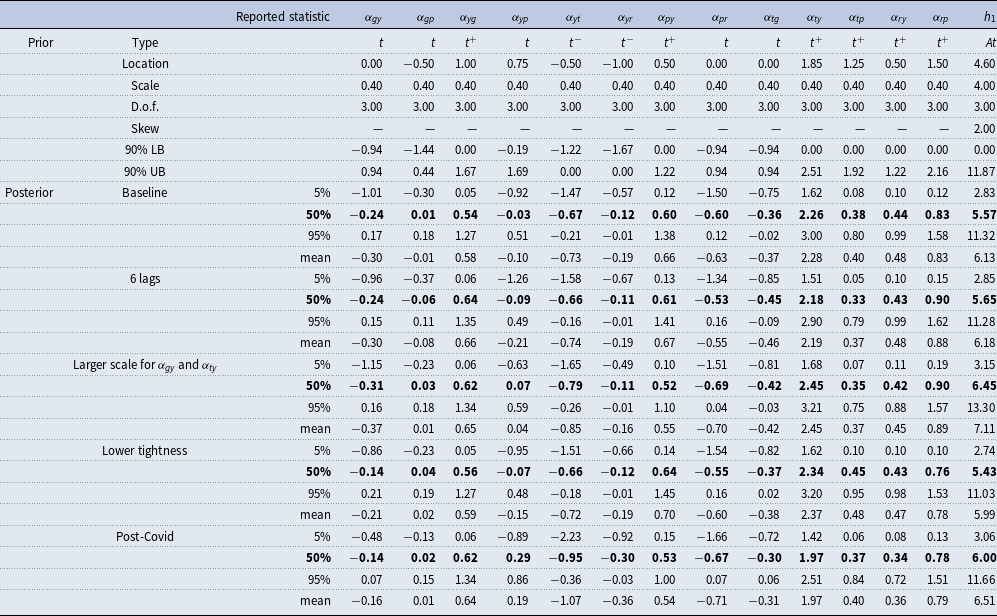

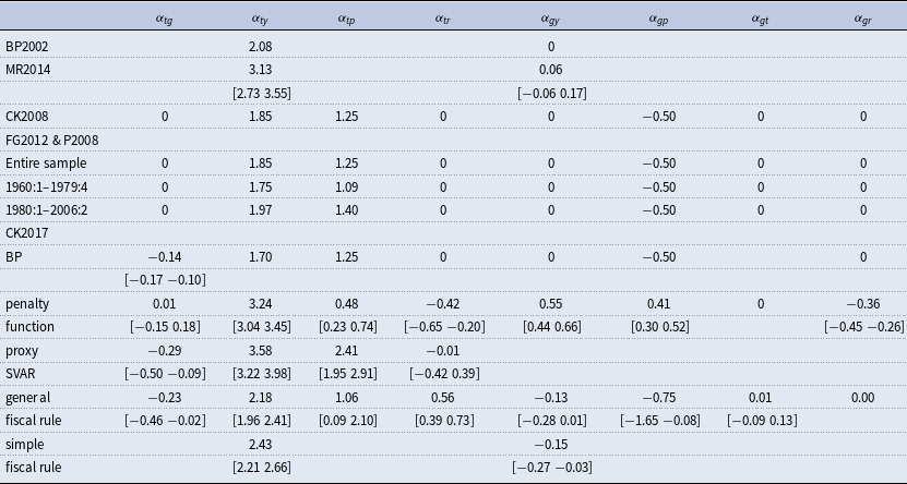


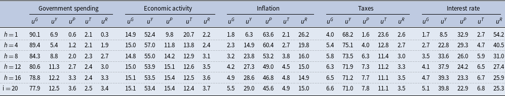
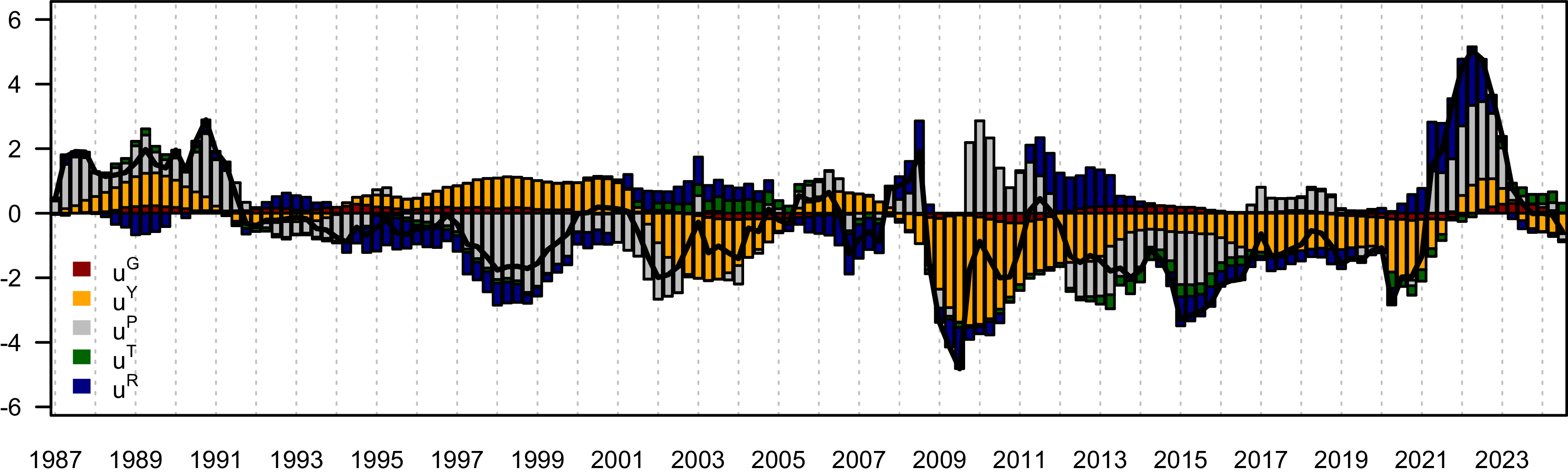


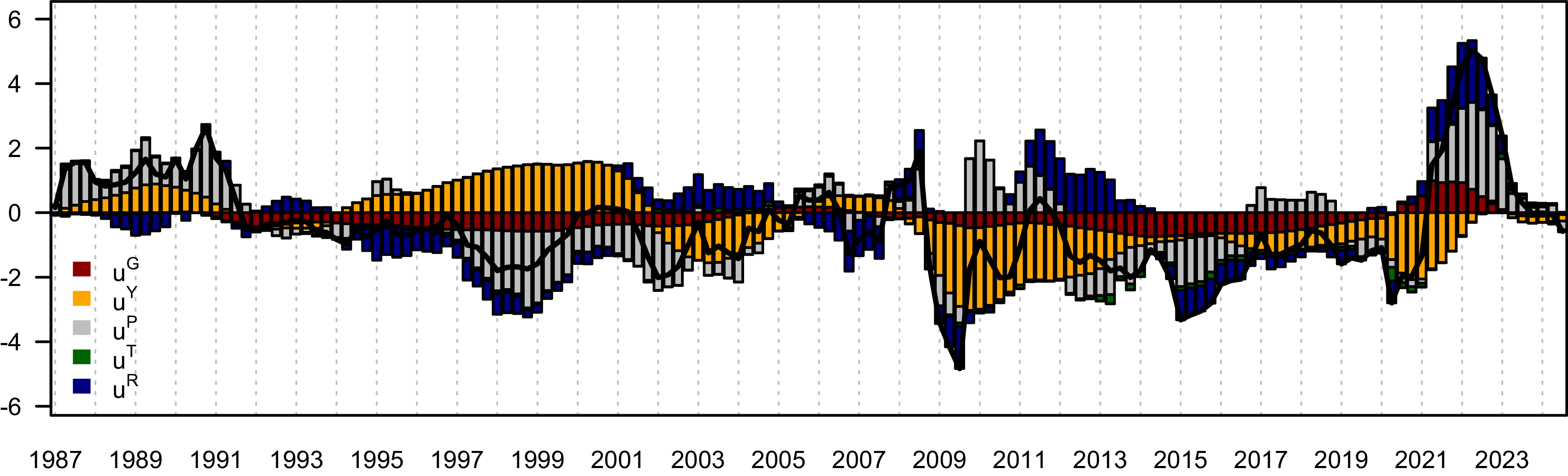
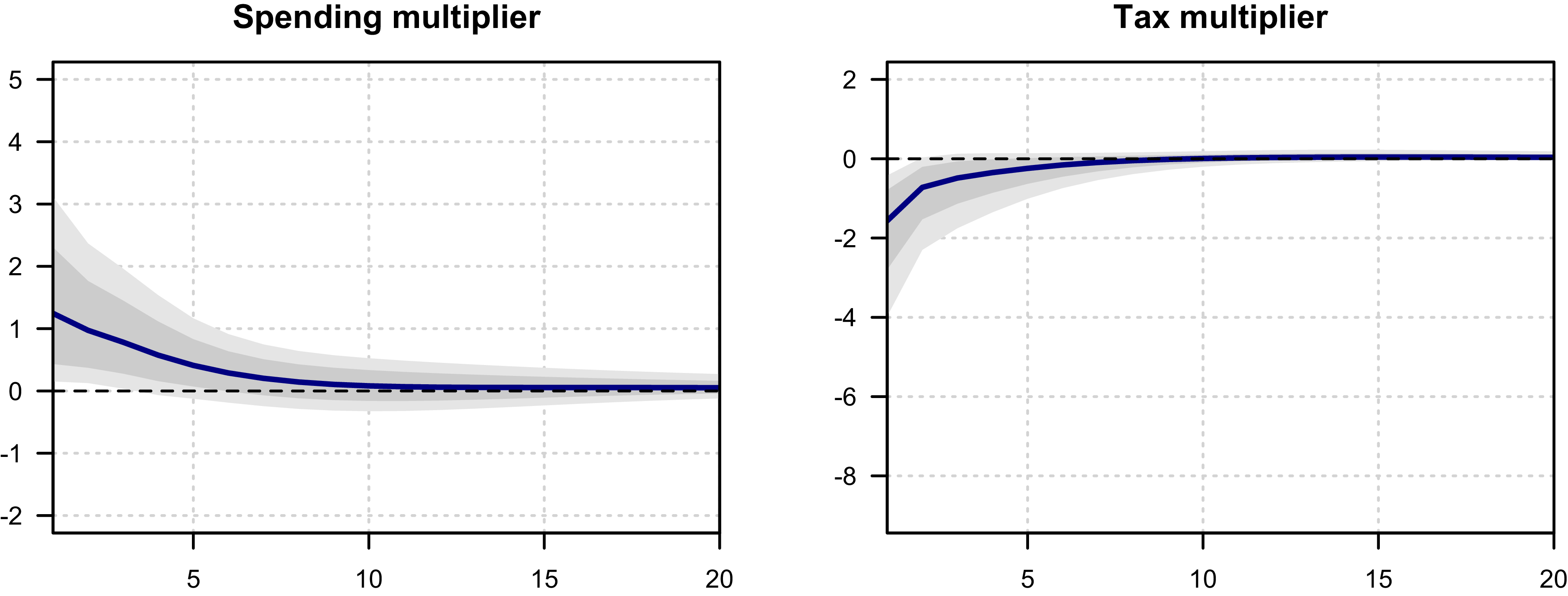
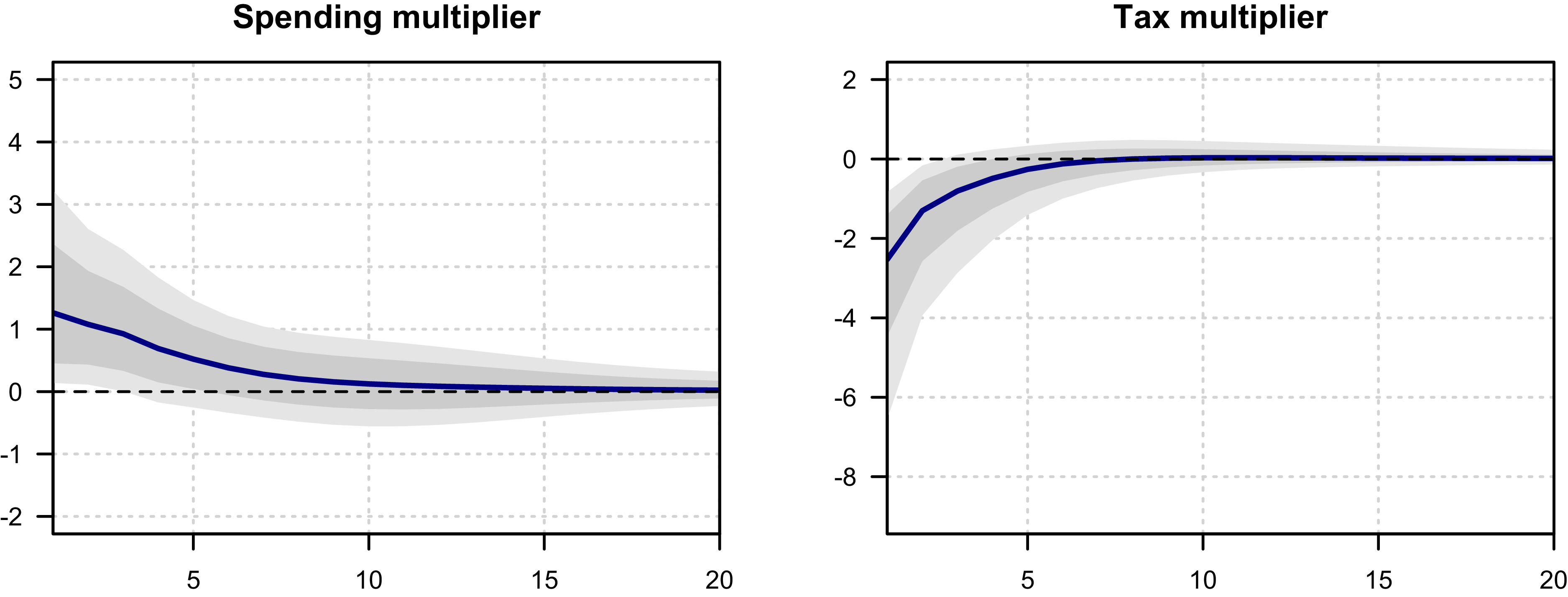
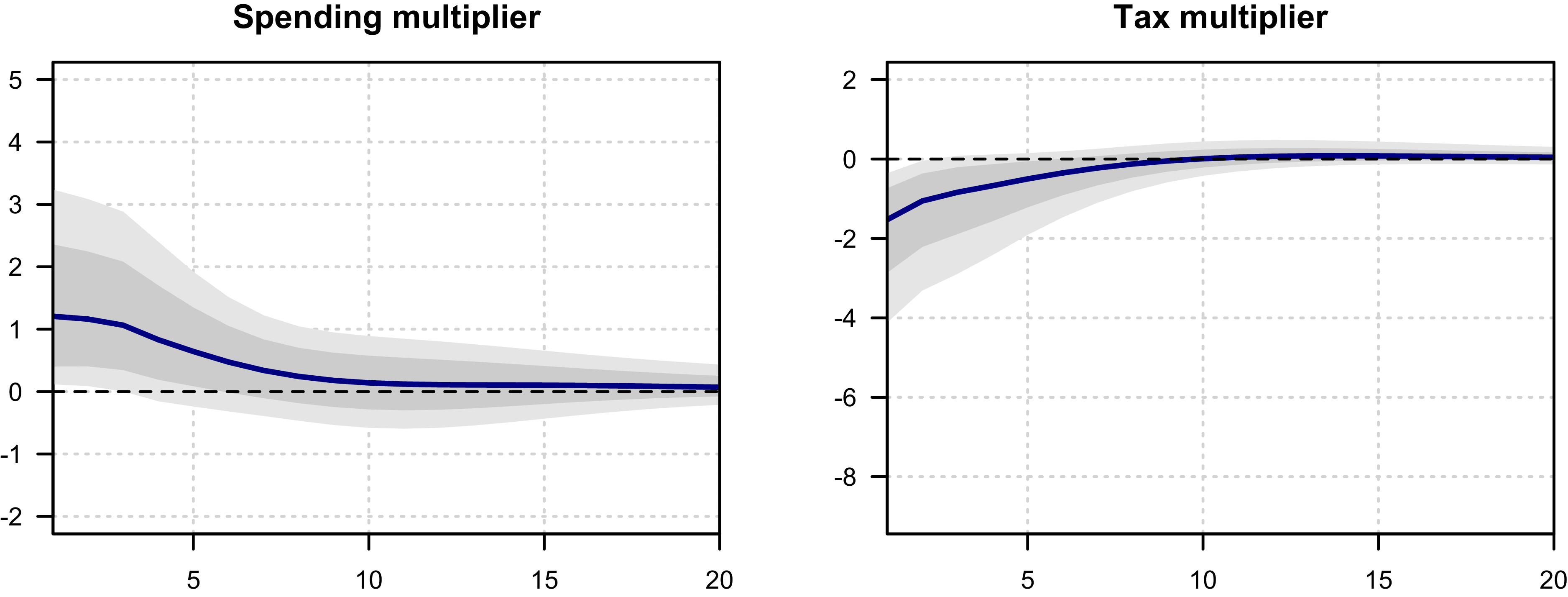
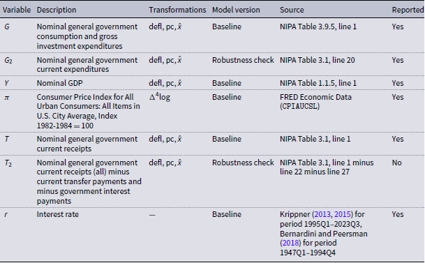

 Open access