


1. Introduction
This paper studies a small, open, overlapping-generations model where the fertility rate and old agents' labor supply are endogenously determined. Reflecting the recent trend that retirement age is increasing and the elderly can be more flexible in their choice of when to retire, we extend the model of van Groezen et al. (Reference van Groezen, Leers and Meijdam2003) by adding endogenous retirement. Given that agents do not internalize the effect that their fertility and labor supply in old age decision may have on the economy, a decentralized equilibrium in this model is not necessarily socially optimal. Thus, we discuss government policies through which equilibrium allocations coincide with socially optimal ones. In particular, we show the role of a child allowance scheme and of a subsidy to elderly labor supply.
The motivation behind our analysis is the increasingly aged population in most developed countries, which has required various continuous reforms to the pension systems in order to ensure sustainability. The extent of the concern over this issue has led many researchers to examine appropriate ways to ensure the economic and political sustainability of social security systems financed on a PAYG basis.Footnote 1
One strand in the literature focuses on policies devoted to increasing fertility in order to ease the burden of demographic change. According to this literature, in a PAYG pension system, parents do not take into account the externalities produced by fertility and, therefore, this leads to a sub-optimal fertility rate. In particular, fertility choices are associated with three social externalities: the intergenerational transfer effect, the child quality effect, and the capital dilution effect (Cipriani, Reference Cipriani2014). The first effect arises from the fact that a higher fertility rate increases the number of future workers who can then support pensioners. However, agents do not take into consideration this positive effect on pensions and this leads to a market equilibrium with an insufficient number of children (see among others Nishimura and Zhang, Reference Nishimura and Zhang1992; Cigno and Rosati, Reference Cigno and Rosati1996; Ehrlich and Lui, Reference Ehrlich and Lui1998; Cigno, Reference Cigno2006, Reference Cigno2009; Cremer et al., Reference Cremer, Gahvari and Pestieau2006). The child quality effect is related to the parental choice of investment in their children's human capital. Higher investments in children's education raise the return of a PAYG pension system because the increase in tax revenues generated by higher future wages can be allocated to the pension system (see Meier and Wrede, Reference Meier and Wrede2010; Cremer et al., Reference Cremer, Gahvari and Pestieau2011). Finally, the third effect is the capital dilution externality and goes in the opposite direction: a higher fertility rate reduces the capital-labor ratio and therefore also the per capita income and pension benefits (see Michel and Pestieau, Reference Michel and Pestieau1993; Cigno, Reference Cigno1993).
The literature highlights two main policy instruments that can be used to internalize these fiscal externalities: child allowances and fertility-related pensions. Regarding the first instrument, van Groezen et al. (Reference van Groezen, Leers and Meijdam2003) and Yasuoka and Goto (Reference Yasuoka and Goto2011) show that, in a small open economy with endogenous fertility and a PAYG pension system, introducing a child allowance enables the first-best level of fertility to be attained and leads to a Pareto improvement. Van Groezen et al. (Reference van Groezen, Leers and Meijdam2003) also discuss the reduction of PAYG contributions, combined with a debt policy that compensates the first generation of pensioners, as an alternative policy. However, this kind of reform does not lead to a Pareto improvement as it would not raise the utility of all generations. Following the same approach, van Groezen and Meijdam (Reference van Groezen and Meijdam2008) show that in a closed economy introducing a child allowance scheme increases fertility, but it is not Pareto improving, because while the utility of the young increases, the utility of future generations decreases due to the capital dilution effect. Fenge and Meier (Reference Fenge and Meier2005) demonstrated that fertility-related pensions are equivalent to child benefits as instruments for achieving the optimal number of children in a PAYG pension system. Fanti and Gori (Reference Fanti and Gori2013) show that in an overlapping-generation model, the introduction of fertility-related PAYG pensions can destabilize the economy and lead to chaotic dynamics. Moreover, Fanti and Gori (Reference Fanti and Gori2014) show, in contrast to van Groezen et al. (Reference van Groezen, Leers and Meijdam2003), that in an overlapping-generation economy characterized by public pension systems, endogenous fertility, and longevity, the steady-state welfare can be maximized with the introduction of a child tax. Along these lines, Stauvermann and Kumar (Reference Stauvermann and Kumar2018) show that in a framework with both endogenous education and fertility, while the provision of an educational subsidy is welfare-enhancing, the introduction of child allowances is not.
Overall, this strand of literature focuses on fertility and child-related policies, but does not take into account retirement choices and therefore does not consider possible policies for increasing the labor supply in old age. To the best of our knowledge, no study, until now, has analyzed the optimal policies that aim to attain the first-best allocation and their welfare implications in a model including both endogenous fertility and endogenous retirement choices. This allows us to focus on the joint effects of policies devoted to internalizing the social externalities of both fertility and labor supply in old age. In particular, the introduction of endogenous retirement allows us to analyze the effects of policies which are very near to the leading reforms implemented by various governments in recent years to ensure the financial sustainability of their respective pension schemes.
Most of the literature focuses on the link between endogenous labor participation in old age and life expectancy without taking into consideration fertility choice (see, e.g., Aísa et al., Reference Aísa, Pueyo and Sanso2012; Cipriani, Reference Cipriani2014; Nishimura et al., Reference Nishimura, Pestieau and Ponthiere2018). A very recent paper which considers retirement policies in a model with endogenous fertility is Cipriani and Pascucci (Reference Cipriani and Pascucci2020). However, in their framework, retirement is exogenous and they do not focus on the first-best policies. Cipriani and Fioroni (Reference Cipriani and Fioroni2019) set up a unified model with both endogenous fertility and endogenous retirement choices in order to compare the effects of different retirement regimes, but they do not examine potential government policies to replicate the first-best allocation. Very few recent contributions, such as Michel and Pestieau (Reference Michel and Pestieau2013) and Miyazaki (Reference Miyazaki2019), focus on policies that aim to achieve the first-best allocation in the presence of endogenous retirement choices but they ignore fertility. Michel and Pestieau (Reference Michel and Pestieau2013) show that the increase in the size of social security benefits negatively affects the elderly labor supply and that the first-best allocation can be implemented only by controlling both the PAYG social security tax and the retirement age. Miyazaki (Reference Miyazaki2019) builds on the Michel and Pestieau (Reference Michel and Pestieau2013) setting by adding the assumption that labor productivity depreciates. Under this setting, Miyazaki (Reference Miyazaki2019) shows that when elderly labor productivity is low, the PAYG pension system alone is enough to implement the first-best optimum in a market economy.
Finally, only the very recent paper by Chen and Miyazaki (Reference Chen and Miyazaki2018) develops an overlapping-generations model to examine the effects of PAYG pension systems and child allowances on fertility, the elderly labor supply, and welfare. However we, on the other hand, focus on alternative government policies aimed at replicating the socially optimal allocation in a market economy initially characterized only by a PAYG pension system. In particular, we consider a small open economy where agents live three periods and both fertility and retirement choices are endogenous. In accordance with the above literature, we find that in a decentralized equilibrium, agents choose to have a sub-optimal number of children. Moreover, agents do not have the appropriate incentive to choose an optimal level of labor supply. Three possible mechanisms may explain this result. First, according to the existing literature, social security provisions lead agents to retire early by reducing the marginal cost of leisure (Gruber and Wise, Reference Gruber and Wise1998). Second, in a PAYG pension system, the elderly do not internalize the positive effect of their labor supply on pension benefits, through higher tax revenues, and therefore choose a sub-optimal labor supply. Finally, agents fail to consider that a higher labor supply, for a given aggregate saving and fertility rate, lowers the capital-labor ratio. This can lead to a higher retirement age than is optimal.
We conclude that governments can achieve the first-best allocation by introducing a child allowance plan to internalize fertility externalities and by subsidizing the labor supply of older people. As an alternative to the latter, governments can achieve the first-best allocation by direct control of the retirement age. Finally, the model is simulated to see whether such policies could be Pareto improvements in an economy initially characterized by two alternative scenarios: (i) a fixed retirement age, i.e., agents retire at the beginning of old age; (ii) flexible retirement age, i.e., agents can choose when to retire. In particular, starting from fixed retirement, the first-best outcome can be realized through a policy consisting of a child benefit scheme and either a mandatory increase in the retirement age or free retirement combined with a subsidy for the elderly labor supply. Starting from a free retirement scenario, the command optimum can be implemented through a policy mix including a child allowance scheme and a subsidy for the labor supply of the elderly.
To sum up, in an economy initially characterized by a mandatory early retirement scheme, the policies considered lead to a Pareto improvement. Indeed, the lifetime utility of current young and future generations increases due to the increase in fertility and consumption and the welfare of today's elderly increases because, despite later retirement, they have higher consumption and increased pension benefits. By contrast, starting from a free retirement regime, a policy including a child benefit plan and a subsidy for the elderly labor supply is not a Pareto improvement. This is due to the fact that, if on the one hand, such a policy increases the welfare of the current young, on the other hand, it negatively affects the welfare of the current elderly because the introduction of a child benefit scheme lowers the resources available for pensions.
The structure of the paper is the following: the next section sets out some stylized facts regarding recent demographic trends and pensions. Section 3 presents the basic model, Sections 4 and 5 show, respectively, the first-best and the decentralized solutions. Section 6 compares the market and the first-best allocation, focuses on the alternative policies available to governments in order to realize the social optimum in a market economy and provides a numerical example in order to study whether these alternative policies could lead to Pareto improvements. The final section summarizes our results.
2. Background
In the past decade, although pension reforms have been widespread in all OECD countries, concerns remain regarding the financial sustainability and pension adequacy of the current pension systems due to the projected increase in the aging population (OECD, 2017). In the period 1975–2015, the combination of rising life expectancy and low fertility rates led on average, in OECD countries, to an increase in the old age dependency ratio of nearly 40% and it is expected to reach 58.6 by 2080 (see Figure 1).
Old-age dependency ratio. Source: OECD (2017).

The continuous change in the age structure drives the need for ongoing adjustments to the pension system. In particular, the leading reforms of various governments in recent years have involved changes to benefits, contributions, tax incentives, the raising of the retirement age, and free retirement schemes (see Galasso and Profeta, Reference Galasso and Profeta2004). As a result of these institutional reforms, the average effective retirement age, in OECD countries, which went down from 1970 to the early 2000s, has been on the increase since the start of the 21st century although it remains significantly below the 1970 level (see Figure 2).Footnote 2
Average effective age of retirement – years in retirement, OECD countries (1970–2017). Source: OECD (2017).
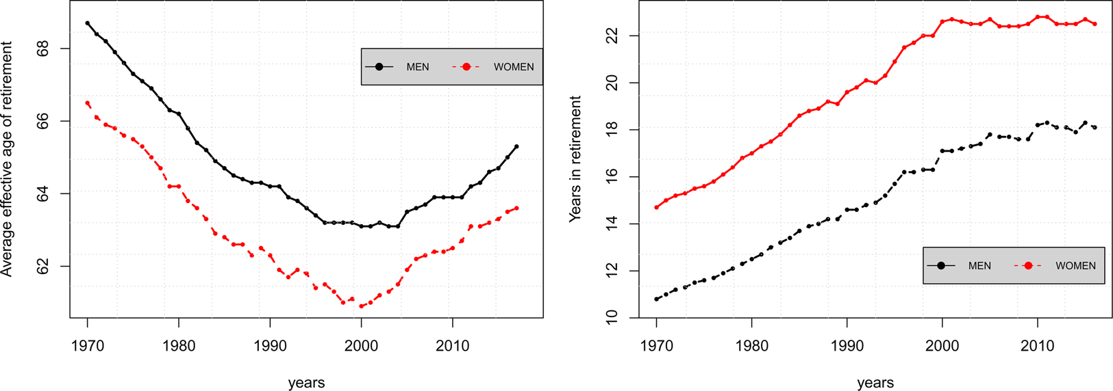
According to OECD estimates, on the basis of current legislation, the normal retirement age for a person who enters the labor force aged 20 should increase on average over the next four or five decades from 64.3 in 2016 to 65.8 years for men and from 63.4 to 65.5 years for women, across all OECD countries (OECD, 2017).Footnote 3
The right-hand panel in Figure 2 shows that the increased exit age in the labor market since 2000, counterbalancing the increase in life expectancy, has stabilized the duration of retirement at around 22 years for women and 18 for men.
In recent years, in order to increase the labor supply of older workers, governments have carried out pension reforms which are intended to promote flexible retirement schemes allowing individuals to choose when and how to retire. In particular, flexibility can include partial retirement, i.e., the ability to combine work and pensions. All European countries allow pensioners to engage in paid work, but the European Labor force survey shows that, in 2012, only about 10% of individuals between the ages of 60–64 and 65–69 in fact chose to combine work after retirement. Another element of flexibility is the choice of retirement age. Most pension systems already offer this flexibility by allowing early retirement, although this has been reduced over the last few decades to improve the financial sustainability of pension systems. Indeed, in recent years, in many countries, pension system reforms have moved in the opposite direction, allowing and incentivizing workers to defer retirement.
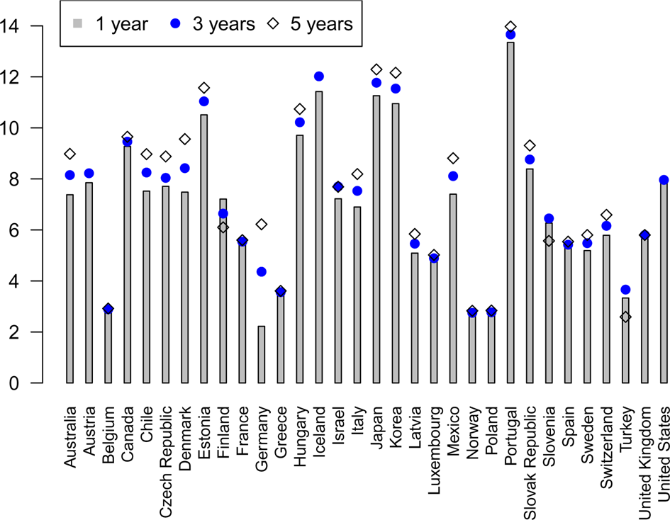
Figure 3 indicates that in the vast majority of OECD countries, postponing retirement leads to higher pension benefits. Specifically, it shows the impact of the deferral rate, additional entitlements, and the benefit as the proportion of total annual benefits for a full-career worker. On average, there is an increase of about 6.8% per year in deferrals, which ranges from a minimum of 2.2% in Germany to a maximum of 13.35% in Portugal. Moreover, the length of the deferral period does not significantly influence the increase in benefits; while a deferral of 1 year on average increases pensions by 6.8%, a deferral of 5 years leads to an increase of 7.3%.
Impact of postponing retirement on annual pension benefits. Source: OECD (2017).
Despite financial incentives for retirement deferral and the introduction in many countries of pension penalties for early retirement, people nonetheless commonly retire early in many OECD countries.Footnote 4 Indeed, although early retirement declined in some countries between 2006 and 2014, the decrease in OECD countries on average has been relatively low about 7 − 8% (see Figure 4). Thus, a crucial question for governments is whether flexible retirement schemes for promoting the elderly labor supply are actually effective (see OECD, 2017). In fact, on the one hand, they incentivize agents to work longer and increase total tax revenues given the contributions from the elderly workforce and, on the other hand, flexible retirement can encourage agents to retire early if they underestimate their future financial needs. Moreover, the ability to combine work and pensions can cause some people to reduce their working hours. Thus, the overall impact of flexible retirement on total hours worked is unclear and in some cases it is the opposite of what could be expected (for a detailed analysis of this point, see Börsch-Supan et al., Reference Börsch-Supan, Bucher-Koenen, Kutlu-Koc and Goll2018).
Early retirement OECD countries. Source: OECD (2017).

3. The model
We assume an economy with overlapping generations of people who live for three periods. In childhood, individuals make no decisions; in adulthood, they work full-time and raise their offspring. In old age, they either continue working or retire. In the latter case, they benefit from a state-funded PAYG pension scheme. For the sake of simplicity, the length of each period is normalized to one.
An adult in period t (and therefore elderly in period t + 1) derives utility from consumption in adulthood, i.e., $c_t^y$ , the number of childrenn t, and from consumption in old age $c_{t + 1}^o$
 and leisure time (1 − l t+1) after retirement. Therefore, the utility function is given by:

where β ∈ (0, 1) is the overall weight attached to utility in old age, δ ∈ (0, 1) is the weight of retirement, and θ reflects fertility preferences.
A small open economy is considered, with perfectly mobile capital. This means that the interest rate is equal to the world interest rate r which is assumed to be constant over time. On the assumption that production occurs according to a constant-returns-to-scale technology, i.e., $Y_t = AK_t^\eta L_t^{1-\eta }$ , capital per unit of effective labor and the wage w are fixed and constant over time. The labor supply in each period t comprises N t = n t−1N t−1 adult workers who supply one unit of labor and old workers each supplying l t, i.e., N t−1l t. In equilibrium, this supply must be equal to the total demand, i.e.:

4. The first-best solution
This section describes the first-best allocation. Consider a central planner who aims to maximize the lifetime utilities of all current and future generations. The social welfare function is, therefore, given by:

where 0 < α < 1 is the social discount factor.
Assuming that capital does not depreciate, the total resources of the economy, comprising production and debt creation minus interest payments, are devoted to the consumption of the young and old, the cost of raising children q and domestic investments:

where R = 1 + r, k = K/L is the capital-labor ratio, and d t is the per capita foreign debt of the country at timet.Footnote 5
Maximizing (3) at time t subject to the economy's resources constraint (4) yields the following first-order conditions:


Equations (6) and (7) show, respectively, the optimal intergenerational allocation, i.e., the equality of the marginal utility of the young generation in two different periods, and the optimal intragenerational allocation, i.e., the equal marginal utility of consumption in the young and old generations. Equation (8) gives the optimal relationship between fertility, consumption at the young age, and labor supply in old age. Equation (9) indicates that, as an optimum, a corner solution for labor supply in old age arises if the marginal cost of leisure in old age is lower than its marginal utility.
It should be noted that the feasible set in the welfare optimization problems may not be convex and therefore the first-order conditions above are necessary, but not sufficient for the solution to be a maximum (see Abio et al., Reference Abio, Mahieu and Patxot2004; Conde-Ruiz et al., Reference Conde-Ruiz, Giménez and Pérez-Nievas2010; De La Croix et al., Reference De La Croix, Pestieau and Ponthière2012; Fanti and Gori, Reference Fanti and Gori2012; Yew and Zhang, Reference Yew and Zhang2013; Li and Zhang, Reference Li and Zhang2015). Thus for the solution to be a social optimum, we assume:
Assumption 1 α < α < θ and qR < w < (qR 2 + Ψ)/(1 + R),
where α = θ/(1 + θ + β) and Ψ are given in Appendix A where more technical details can be found.
Thus under Assumption 1, from Equations (6)–(9), the first-best allocation is:


Finally, if the preference for retirement is sufficiently high, i.e., $\delta \ge \hat{\delta }$ , with $\hat{\delta } = w[ {\alpha ( {1 + \theta + \beta } ) -\theta } ] {\rm /}[ {\alpha \beta R( {w-qR} ) } ]$
 , then a corner solution with full retirement arises:


Note that a higher social discount factor implies a higher threshold level $\hat{\delta }$ . Thus if the social planner is more patient, then it is more difficult that a corner solution for elderly labor supply arises.
5. A decentralized economy
This section analyzes the optimal allocation in a market economy in the presence of a PAYG pension system. As adults, agents allocate their wages to consumption $c_t^y$ , savings s t, raising their children n t, and paying a payroll tax τ in order to contribute to a PAYG pension. The budget constraint of an adult agent in period t is, therefore, given by:

where q > 0 is the cost of raising each child. In the third period, agents consume their savings, receive a pension benefit b t+1 over the period in which they do not work, and when they work pay income tax τ in order to finance the PAYG pension scheme. Thus, the budget constraint in old age is as follows:

In period t + 1, the size of the adult population is N t+1 = n tN t and the size of the elderly is $N_{t + 1}^o = N_t$ . Total tax revenues are collected by the government to finance social security benefits. Assuming a balanced budget regime in each period, pension benefits in period t + 1 are:

Each household chooses n t, s t, and l t+1 to maximize the utility function (1) subject to (16) and (17) and l t+1 ≥ 0 taking as given the wage, interest rate, and pension benefit. The first-order conditions are given by:


Equation (19) is equivalent to Equation (7), indicating that the savings decisions of agents are consistent with a centralized economy whereas Equation (20) differs from social planner's one given by Equation (8). In fact, the marginal utility of fertility does not take into account the terms β and the interaction with the labor supply in old age, i.e., f(k)l t+1/Rn t. Differently from the central planner, agents discount future consumption at the rate β and do not take into account the fact that having a higher number of children implies a higher aggregate output shared by the same number of pensioners in the future. Similarly, they do not consider that a later retirement period, for a given number of children, increases total output shared by a given number of pensioners. Both of them constitute a dependency ratio effect.
Moreover, parents do not consider the effective cost of having an extra child, which is not just q but q + k − d t+1 because when the number of children increases, savings and/or the foreign debt should increase in order to keep the capital-labor ratio at the same level (see van Groezen et al., Reference van Groezen, Leers and Meijdam2003). Finally, Equation (21) differs from the social planner's one because, other things being equal, social security decreases the relative price of leisure in old age.
From the first-order conditions, we obtain the interior solution:


and

On the other hand, if the agents' weight on the preference over leisure when old is sufficiently high, i.e., δ > δ, with δ = [qR(1 + β + θ) − (1 + R)wθτ]/qR 2β, then a corner solution for elderly labor supply arises:


6. First-best allocation versus market allocation
This section compares the first-best allocation with a market economy and discusses potential government policies to implement the first-best allocation in a decentralized economy, both in the corner and the interior solution.
6.1 Corner solution
After replacing b t+1 from Equation (18) in Equations (25) and (26), optimal fertility and young consumption in a steady state and a market economy are given by:

and

where we assume τ < Rq(1 + θ + β)/θw.
Comparing Equations (27) and (28) with (14) and (13), it can be seen that the optimal choices of households differ from those of a central planner. In particular, in accordance with the existing literature (see, e.g., van Groezen et al., Reference van Groezen, Leers and Meijdam2003; Cremer et al., Reference Cremer, Gahvari and Pestieau2011; Cipriani, Reference Cipriani2014), optimal choices in a market economy differ from the social optimum due to two effects. The first, known as the intergenerational transfer effect (or dependency ratio effect), means that in a PAYGO social security system, individuals do not take into account the effect each person's fertility decision has on population growth and therefore on everybody's pension benefits. In other words, they do not take into account that a higher number of children means that, in the future, there will be a higher number of workers able to support pensioners. This leads to a decentralized equilibrium with too few children. The second effect is the capital dilution effect: parents do not consider that a higher fertility rate, given the aggregate saving, lowers the capital-labor ratio. In a small open economy, the capital-labor ratio is constant and thus, if the number of children increases, savings and/or foreign debt should increase in order to maintain the capital-labor ratio at the same level. This leads to a decentralized equilibrium with too many children. Depending on which of these two effects prevails, the number of children in a market economy is either too low or too high compared to the first-best solution.
Thus, the government needs to redistribute resources across generations in order to achieve the first-best allocation in a decentralized economy. Suppose the government provides a subsidy ε t per child in order to lower the cost of raising a child. The budget constraint in adulthood, therefore, becomes:

and assuming that the government devotes a fraction 0 < λ < 1 of tax revenues to child benefits and a fraction 1 − λ to social security benefits, the internal allocation of government expenditure is given by:

and

Thus, the optimum policy combination is τ = τ* and λ = λ*, where:

and

Note that for a given value of the social discount factor, i.e., α 0 = θw/Rq(1 + θ + β), τ* = 0, where α 0 > α. Thus, for this level of the social discount factor, the market outcome coincides with the first-best solution and therefore government intervention is unnecessary. On the other hand, if the social discount factor is sufficiently high, i.e., α > α 0, then in a market economy, the dependency ratio effect (intergenerational transfer effect) dominates the capital dilution effect, i.e., parents have too few children (n* < n**) and this in turn means higher consumption in the decentralized equilibrium c* > c**. Thus, the government should provide a positive child allowance in order to achieve the first-best outcome (see van Groezen et al., Reference van Groezen, Leers and Meijdam2003). By contrast, if α < α 0, children should be taxed in order to achieve the first-best solution.
From Equations (31) and (33), it follows that the first-best allocation is achieved in a market setting if the child allowance equals the present value of the pension benefit, i.e., ε = w(1 − λ*)τ*/R (see van Groezen et al., Reference van Groezen, Leers and Meijdam2003).Footnote 6 This coincides with the level of child allowance that, for a given value of the PAYG-tax τ, maximizes lifelong utility for the young in period t.
6.2 Interior solution
We now turn to the equilibrium where agents choose to supply labor in their old age. Thus, after replacing b t+1 from Equation (18) in Equations (22)–(24), optimal fertility, consumption, and the labor supply in old age, in a steady state, are given by:


As in the case of the corner solution, the optimum choices of households deviate from the social optimum. However, in addition to the intergenerational transfer effect and the capital dilution effect discussed above, the impact of pensions on the labor supply in old age and the interaction between the labor supply in old age and fertility have to be considered. In particular, from Equations (21) and (9), the provision of pension benefits reduces the marginal cost of leisure in old age leading to early retirement. In addition, agents do not take into consideration the fact that a higher labor supply in old age, all else being equal, increases pension benefits and thus, from this point of view, the labor supply in old age is too low. On the other hand, agents also fail to consider that a higher labor supply in old age, for given aggregate savings and fertility, lowers the capital-labor ratio. In a small open economy, the capital-labor ratio is fixed and thus, if the labor supply in old age increases, savings and/or foreign debt should increase in order to maintain the capital-labor ratio at the same level. This leads to a decentralized equilibrium with an excessive labor supply in old age. Thus, depending on which of these effects prevails, the levels of labor supply and fertility in a competitive equilibrium will either be lower or higher than those in the first-best economy.
Therefore, as in the corner solution, to replicate the first-best allocation, the government needs to introduce certain public policies. In particular, the government is able to increase fertility and to decrease the retirement period by a mix of policies that redistribute across generations. Assuming that the government introduces a subsidy or a tax on elderly labor supply, i.e., $\tau ^o \ge0$ , agents' budget constraints in adulthood and in old age become:


and the government budget constraint for pensions and a child allowance scheme is:

and

Thus, in equilibrium, the government can ensure that market allocations coincide with the social optimum by setting τ = τ*, τ o = τ o*, and λ = λ*, where:


and

Notice that when the social discount factor is equal to $\tilde{\alpha }^0 = \theta w( {1 + R} ) {\rm /}qR^2[ {1 + \theta + \beta ( {1 + \delta } ) } ]$ , with $\tilde{\alpha }^0 > \underline{\alpha }$
 , government intervention is not required. With this discount factor, in fact, the intergenerational transfer effect is compensated by the capital-dilution effect and fertility and retirement are at the first-best level. For other levels of α, the command optimum does not coincide with the market solution. In particular, if $\alpha > \tilde{\alpha }^0$
 , parents have too few children and retire too early, i.e., n* < n**, c* > c**, and l* < l**, and therefore the government should provide a child allowance and a subsidy for the labor supply of older people in order to achieve the first-best allocation. On the other hand, if $\underline{\alpha } < \alpha < \tilde{\alpha }^0$
 , fertility and elderly labor supply are too high, a tax on children and elderly labor supply would be required so that agents choose to have a lower number of children and retire early. The relationship between the social discount factor and the sign of the Pigouvian tax goes in the same direction as van Groezen et al. (Reference van Groezen, Leers and Meijdam2003): in general, the market outcome differs from the command optimum depending on whether the intergenerational transfer effect prevails or is dominated by the capital-dilution effect. In our model, in addition to the standard capital-dilution effect of fertility, we have another effect on the capital-labor ratio from the labor supply of old agents. On the other hand, labor supply of older agents could be lower than optimal given its effect on pension benefits.
From Equations (41)–(43), if τ o = τ, it is not possible to achieve the first-best allocation in a decentralized economy. In this case, in fact, the government needs an additional instrument for the market outcome to coincide with the social optimum, particularly direct control of the retirement age. In this case, workers cannot choose the length of their retirement period but are induced by the government to work for a fixed amount of time $\bar{l}$ . Thus, given that τ o = τ, the optimum fertility and consumption chosen by households in the steady stare are implicitly given by:

and

where $\bar{l}$ is given by Equation (12) and $\epsilon ( n ) = \lambda w\tau ( {n + \bar{l}} ) {\rm /}n^2$
 . In this case, therefore, the government can achieve the social optimum in a market economy by setting $\bar{l} = l^{{\ast}{\ast} }$
 , $\tau = \bar{\tau }^\ast$
 , and $\lambda = \overline {\lambda ^\ast }$
 :
:

and

6.3 Can reforms yield a Pareto improvement? A simulation
In this section, we consider an economy initially characterized by a PAYG-pension system, no child allowance (λ = 0), and no subsidy for elderly labor supply (τ o = 0). This could be a typical developed country, which is facing an aging population with the usual pension sustainability problem. We wish to investigate the possibility of implementing a policy to achieve the first-best and in particular, to check if such a policy could be Pareto-improving.
We consider two types of pension systems: one is characterized by a fixed retirement age, and the other by a flexible retirement regime. In the first case, agents retire at the onset of old age, whereas in the second case, agents decide when to retire, provided that they work for a minimum number of years (equivalent to the first period).
In the first case, as we have seen in Section 6, a government can achieve the first-best allocation either through a policy that consists of setting the fixed retirement age at the optimal level (l**) and implementing a child subsidy (policy 1) or through a policy which consists of a subsidy on both the elderly labor supply and fertility (policy 2). Under a flexible retirement regime, the first-best allocation can be achieved by a policy mix that includes both a child allowance and a subsidy for the labor supply of the elderly. In the simulation, we refer to this case as policy 3.
We focus on these pension reforms because, in general, they recall the main policies implemented in recent years by various governments for increasing the financial sustainability of pension systems. In fact, as discussed in Section 2, raising the retirement age has been a common reform over the last two decades in almost all OECD countries. Additionally, various countries have boosted incentives for working longer. For instance, Belgium, Canada, and Denmark have recently been enhancing work incentives for elderly workers (OECD, 2019). Finally, many countries provide various incentives for childcare, often in the form of credits for periods of maternity leave. However, as found by the OECD (2019), on average, these incentives are not enough to compensate women for lost pension income.
Of course, in many countries, the distinction between the policies that we are analyzing is not so clearly defined and often we find more complex scenarios. Thus, our aim is not to provide a comprehensive analysis of complex recent pension reforms, but to shed some light on their potential welfare impact across the generations.
We assume that one period lasts 30 years. The parameter η, that is the capital share in added value, is set at 0.3 as usually assumed. The annual interest rate is set at 1.2% per year and therefore we obtain R = 1.4 over a generation (30 years). The productivity level A is a scale parameter and is set at 1.5 in order to satisfy Assumption 1. Given R, η, and A, the capital-labor ratio is k = 0.2 and this means that w = 0.6. Following Blackburn and Cipriani (Reference Blackburn and Cipriani2002), the annual discount factor is set at 0.99 so β = (0.99)30 = 0.74 over a generation. The weight of leisure relating to consumption in old age δ is set at 0.8. The child raising cost, q, is set at 0.3, in line with the empirical literature on this resource share, which estimates that children account for between 20% and 30% of the households' budget (see, e.g., Letablier et al., Reference Letablier, Luci, Math and Thévenon2009; Apps and Rees, Reference Apps and Rees2001). The initial social security rate is equal to0.15. The parameter θ is calibrated to produce a total fertility rate of 1.2 in the steady state before policy implementation. However, since the model includes single sex individuals in the model, θ is calibrated so that fertility is equal to 0.6 per individual. This gives θ equal to0.85. This parameter set yields$\widetilde{{\alpha ^0}} = 0.65$ , thus we set α = 0.7.
Ten periods (i.e., generations) are considered and the economy is assumed to be in the steady state until period 3, and the new policy is announced and implemented at the beginning of period 4. Thus, until period 3, agents' choices, in the case of policy 1 and 2, are given by Equations (27) and (28), while in the case of policy 3, they are given by Equations (34)–(36).
Figure 5 shows the impact of the three policies on the utility of the currently young and all future generations.
Welfare analysis. Policy 1 consists of setting the fixed retirement age at the first-best level (l**) and implementing a child subsidy; policy 2 consists of a subsidy for both the elderly labor supply and fertility in a fixed retirement regime; policy 3 consists of a child allowance and a subsidy for elderly labor supply in a flexible retirement regime.

The black curve refers to lifetime utility in the case of policy 1. Here, the government sets $\bar{l} = l^{{\ast}{\ast} }$ and imposes a tax rate $\tau = \bar{\tau }^\ast$
 and $\lambda = \overline {\lambda ^\ast }$
 (see Equations (46) and (47)). With our parameters set, we obtain $\bar{l} = 0.57$
 , $\bar{\tau }^\ast{ = } 0.13$
 , and $\overline {\lambda ^\ast } = 0.25$
 .Footnote 7 From period 4, agents change their fertility and consumption choices and this implies an upward spike followed by a small decrease in periods 5–6 which then stabilizes at the first-best level from period 6 onwards. In fact, both fertility and consumption do not immediately reach the first-best level because they negatively depend on the fertility choices of the previous period.Footnote 8 Overall, lifetime utility increases compared to the initial steady state. The introduction of a child allowance actually lowers the cost of raising children and thus, all else being equal, increases the fertility and consumption of young agents (see Figure 6 in Appendix B). Moreover, forcing agents to work in old age has both a direct positive income effect and an indirect positive effect, through child allowance, on fertility (see Equation 44). Finally, the reduction in the retirement period reduces the necessity of savings, thus increasing consumption in adulthood. To sum up, utility increase from higher fertility and consumption exceeds the utility loss from the reduction of leisure time in old age. In order to give a measure of welfare change, we calculate the wealth equivalent. Specifically, this is a measure of the percentage increase in full lifetime resources needed in the initial scenario, without the policy, to achieve the level of utility reached after the introduction of the policy (Auerbach et al., Reference Auerbach, Auerbach and Kotlikoff1987; Fehr et al., Reference Fehr, Kallweit and Kindermann2017). Overall, we find that welfare gains from the initial steady state to the final one, measured in terms of wealth equivalent, amount to 24%.
However, what is most interesting to study is the effect of this policy on the welfare of the current elderly. Clearly, the effect is a priori ambiguous, since on the one hand, it increases their retirement age, which has a direct negative effect on utility, and on the other hand, it increases their labor income and pension benefits. Overall, in our example, for currently elderly agents, the gain in welfare is equivalent to a variation in wealth of 22%.
In policy 2, the government starting from a mandatory retirement system allows agents to choose how much they wish to work in old age, providing them with a subsidy in order to raise the elderly labor supply to the first-best level. Thus, from Equations (41)–(43), with our parameters set, we obtain τ* = 0.13 and λ* = 0.62, τ o* = −0.07. Lifetime utility follows a very similar path to policy 1, and therefore as in policy 1, there is a marked increase in lifetime utility in period 4 due to the positive impact of child benefit and the possibility of working in old age, on fertility and consumption. Regarding the currently elderly, as in the case of policy 1, there are two opposite effects on utility, that is, a positive one due to a higher consumption and a negative one due to the reduction of leisure time in old age. The total effect on the currently elderly is positive and is equivalent to a variation in wealth of 33%.
Thus, comparing policy 1 and 2, we can observe that although both lead to the same welfare gain for the currently young and future generations, because the total value of lifetime resources in the initial scenario is the same, policy 2 implies a higher welfare gain for the currently elderly. This is due to the fact that, while in policy 1 labor supply is immediately taken by the government to the first-best level, in policy 2 although the subsidy to the elderly labor supply induces agents to delay their retirement period, this is, nevertheless, above the first-best level. This, therefore, implies a minor utility loss.
Finally, regarding policy 3, there is an increase in lifetime utility, albeit smoother and lower compared to the previous policies. Indeed, in this case, agents already have the opportunity to work in old age prior to the introduction of the policy, and therefore, when compared to a scenario initially characterized by mandatory early retirement, fertility is higher and although the policy has a positive effect, the increase is lower (see Figure 6 in Appendix B). In fact, while in policies 1 and 2, the positive income effect of the labor supply in old age adds to child benefit, in policy 3, this additional effect is missing. Thus, the welfare gain from the initial steady state to the final one, measured in terms of wealth equivalent is 6%.
Regarding the currently elderly, policy 3 leads to a reduction of their welfare, i.e., −2.7%. This is due to the relatively low increase in consumption because, although the subsidy to elderly labor supply, on the one hand, has a direct positive effect on consumption, on the other hand, it has an indirect negative effect through a lower pension benefit. In particular, the latter decreases because total tax revenues, i.e., $\tau + \tau ^ol_t^\ast {\rm /}n_{t-1}^\ast$ , decrease and this in turn implies an increase in the fraction of tax revenues devoted to child benefit, i.e., λ, necessary for taking fertility to the first-best level.
To conclude, on the basis of our analysis, while policies devoted to increasing retirement age and child benefits may have a positive welfare effect across all the generations in those countries that are initially characterized by an early mandatory retirement regime, they may, however, generate a worsening of welfare for some generations in countries initially characterized by a flexible retirement regime.
7. Conclusion
In the recent decades, in the vast majority of developed countries, governments have introduced various reforms of their pension systems in order to meet the challenges presented by an increasingly aging population. In particular, the main reforms introduced over the past few years have involved changes to benefits, increases in the retirement age, and the introduction of flexible retirement schemes. In order to study the impact of some of these government policies, a small, open, overlapping-generations economy is developed, characterized by a PAYG social security plan combined with retirement and fertility choices, both of which are endogenous. The result is that parents do not make fertility and retirement choices that coincide with the social optimum because, in a PAYG pension system, they do not consider the nature of public goods, and therefore of the external social effects, of both fertility and the labor supply in old age. We therefore study alternative policies which allow governments to achieve the first-best allocation. In particular, governments can achieve the first-best optimum with an appropriate child benefit plan and either by controlling the retirement age or by introducing a free retirement system combined with subsidies to elderly labor supply.
To provide some clues as to the potential feasibility of these policies, the model is simulated to study whether these policies can lead to a Pareto improvement. Overall, with our parameters set, we find that in an economy initially characterized by a mandatory early retirement system, the introduction of a child allowance scheme and either a mandatory increase in retirement age or a free retirement scheme combined with a subsidy for elderly labor supply is found to be a Pareto improvement. By contrast, in an economy initially characterized by a free retirement scheme, a policy which introduces both a child benefit plan and a subsidy to incentivize the elderly labor supply does not lead to a Pareto improvement.
The model can be extended in various interesting ways. First, a straightforward extension might be the introduction of longevity in order to study the possible effects of its increase on optimal policies (see, e.g., van Groezen and Meijdam, Reference van Groezen and Meijdam2008). Second, another interesting extension could be to remove the assumption of a small open economy. This would certainly enrich the model because – as we are aware – these results may change in an economy with endogenous factor price (see, e.g., Cigno, Reference Cigno1993) although this would complicate the analysis. In addition, along the lines of Miyazaki (Reference Miyazaki2019), the model could be extended to include elderly agent's labor productivity. In this case, controlling the retirement age could have different implications on welfare. For example, when the labor productivity of the elderly workers is very low, encouraging them to retire early could increase welfare (see Miyazaki, Reference Miyazaki2019), and the opposite may be true if their productivity is sufficiently high.
Work will be carried out in the future on all of these possible extensions.
Acknowledgment
We thank the two anonymous referees and the Editor for their helpful comments. We also thank Davide Fiaschi for helpful comments and suggestions.
Conflict of interest
None.
Appendix
A. Second-order conditions
A sufficient condition that guarantees a unique and global maximum is that the planner's objective is strictly concave, in other words, the Hessian matrix should be negative definite at all points (see, e.g., Abio et al., Reference Abio, Mahieu and Patxot2004). The Hessian matrix of the second-order derivatives associated with the planner problem can be written as (see, e.g., Abio et al., Reference Abio, Mahieu and Patxot2004; De La Croix et al., Reference De La Croix, Pestieau and Ponthière2012; Stelter, Reference Stelter2016):

The Hessian matrix is negative definite if the first- and third-order leading principal minors are negative and the second- and fourth-order ones are positive. These, after substituting the first-order conditions, are given respectively by:


where:

The concavity of the utility and the production function guarantees that the first and the second leading principal minors have the right signs.
On the other hand, the third and fourth principal minors need restrictions on parameters in order to be satisfied. In particular, the condition θ > α ensures that the third leading principal minor is negative and the fourth leading principal minor is positive. Finally, by substituting c y from Equation (11) into Equation (52), we find that the determinant of the Hessian matrix is positive if w < (qR 2 + Ψ)/(1 + R) where:

In the case of corner solution for elderly labor, we have a 3 × 3 Hessian matrix and the first-, second-, and third-order leading principal minors are given, respectively, by Equations (48)–(50). Hence, this matrix is negative definite.
B. Simulation
Figure 6 shows the path of fertility under the three possible policies considered in Section 6.3.
Fertility. Policy 1 consists of setting the fixed retirement age at the first-best level (l**) and implementing a child subsidy; policy 2 consists of a subsidy for both the elderly labor supply and fertility in a fixed retirement regime; policy 3 consists of a child allowance and a subsidy for elderly labor supply in a flexible retirement regime.


 Open access