


1. Introduction
The polar regions are highly responsive to changes in climate, and the polar cryosphere in particular has acted as an early warning for climate impacts that have extended to lower latitudes. Ice shelves are features of the high Arctic that are experiencing irreversible change, especially those that fringe the northernmost coast of Ellesmere Island, Severnaya Zemlya, Franz Josef Land and a few northern Greenland fjords (Higgins, Reference Higgins1988; Willis and others, Reference Willis, Melkonian and Pritchard2015; Dowdeswell and Jeffries, Reference Dowdeswell, Jeffries, Copland and Mueller2017). The loss of ice shelves, in the Arctic and Antarctic, may cause acceleration and retreat of tributary glaciers (Wendt and others, Reference Wendt2010; Berthier and others, Reference Berthier, Scambos and Shuman2012; Hill and others, Reference Hill, Carr and Stokes2017, Reference Hill, Gudmundsson, Carr, Stokes and King2020) due to the lessened backstress and may also affect unique ecosystems residing in epishelf lakes (Vincent and Mueller, Reference Vincent and Mueller2020). Therefore, understanding their break-up processes is of utmost importance.
Arctic-style ice shelves form primarily from multi-year landfast sea ice (MYFI) that survives for several decades, thickening to a few tens of meters by snow accumulation and (initially) basal freeze-on. In most cases, there is significant ice input from tributary glaciers, resulting in a mixed-origin ice shelf combining land-ice-sourced areas and in situ accumulated ice (Dowdeswell and Jeffries, Reference Dowdeswell, Jeffries, Copland and Mueller2017).
Arctic-style ice shelves, in the framework of this paper, differ from Antarctic ice shelves in that they are not an extension of a continental ice sheet. They are generally smaller in size and they typically have MYFI as a main component of their total volume (Vincent and others, Reference Vincent, Gibson and Jeffries2001). Arctic-style ice shelves are similar to Greenland glacier tongues (sometimes referred to as ‘ice shelves’) because part of their composition is from tributary glacier ice mass. They differ in that glacier tongues are not sustained by MYFI and are simply an extension of a floating glacier into the ocean. Arctic-style ice shelves are said to take centuries to form (Higgins, Reference Higgins1991), whereas glacier tongues may only take decades. The Matusevich Ice Shelf, in Severnaya Zemlya, is also similar to an Arctic-style ice shelf, however it undergoes a 30-year cyclic break-up (Willis and others, Reference Willis, Melkonian and Pritchard2015) and is therefore different than the sustained century-old Arctic-style ice shelves. Here we will focus on Arctic-style ice shelves only, hereafter referred to as ‘Arctic ice shelves’.
In our study, we identify different regions of ice origin, structure and characteristics as ‘provenance regions’. Arctic ice shelves are typically >20 m thick and are characterized by having quasi-linear surface troughs and ridges with meltwater ponds forming in the toughs in summer (Dowdeswell and Jeffries, Reference Dowdeswell, Jeffries, Copland and Mueller2017). The troughs and ridges have been referred to as ‘rolls’ in previous literature (e.g., Dowdeswell and Jeffries, Reference Dowdeswell, Jeffries, Copland and Mueller2017); here we refer to them as ‘corrugations’. The wavelength of the corrugations has been shown to correlate approximately with ice thickness (Dowdeswell and Jeffries, Reference Dowdeswell, Jeffries, Copland and Mueller2017).
Using strand-line detritus (driftwood and seal carcasses), previous studies determined that the Ellesmere ice shelves formed ~4000 years ago (Vincent and others, Reference Vincent, Gibson and Jeffries2001; England and others, Reference England2008). When first discovered (Peary, Reference Peary1907, Reference Peary1910), a merged ice-shelf fringe extended 500 km along the northern Ellesmere coast. From 1900 to 1982 the Ellesmere Ice Shelf lost over 90% of its area, leaving much smaller individual ice shelves within the fjords (Vincent and others, Reference Vincent, Gibson and Jeffries2001). These ice shelves remained relatively stable until the early 2000s when a series of break-ups began to occur (White and others, Reference White, Copland, Mueller and Van Wychen2015). The last fully intact Ellesmere Ice Shelf, the Milne Ice Shelf, broke up in July 2020 (Vincent and Mueller, Reference Vincent and Mueller2020).
The Hunt Fjord Ice Shelf (HFIS) is the last remaining Arctic ice shelf in northern Greenland and due to poor data availability has not been extensively studied, until now. It is composed of a combination of multi-decadal corrugated fast ice and floating ice tongues. Beginning in 2012, a series of calving events began to disintegrate HFIS. The remaining areas of the HFIS are buttressing several tributary glaciers. A further break-up is likely to cause these glaciers to accelerate due to the lack of backstress provided by the ice shelves (e.g., see Dupont and others, Reference Dupont and Alley2005; Fürst and others, Reference Fürst2016), causing further ice loss through calving and glacial thinning. Additional glacial thinning and retreat may also occur due to basal melting at the grounding line caused by the increased presence of warm subsurface Atlantic Water (Straneo and others, Reference Straneo2012). Unlike several other Arctic ice shelves, HFIS does not have an epishelf lake behind it.
This study uses several remote-sensing datasets to explore the characteristics of HFIS and its provenance regions, and to describe and examine its evolution over the past several decades, including the processes leading to break-up events and their aftermath. The study was initiated by a series of special summer season off-nadir image acquisitions by Landsat 8 spanning 2016–2020 (except 2019) that covered the entire northern coast of Greenland and Ellesmere Island (Figs 1b–e). These were used to determine outlet glacier ice velocities of Hunt Fjord tributaries (Fig. 1c) and to assess the structural characteristics of the ice shelf. Ice, Cloud and land Elevation Satellite (ICESat) and ICESat-2 data, in conjunction with a 1978 photogrammetry-derived digital elevation model (DEM) and the ArcticDEM, are used to assess ice thickness changes on the HFIS over the last few decades (Fig. 1d). Moderate-resolution Imaging Spectroradiometer (MODIS) imagery is used to document the break-up events that began in 2012 (Fig. 1e). We further examine the likely causes of the calving events using both sea-ice extent records and summer melt-day records from passive microwave data (SSM/I-SSMIS).
Overview of the structure of Hunt Fjord Ice Shelf (HFIS) and its evolution since 1978, and summary of the datasets used in this analysis. (a) Subscene of the late summer 1978 airphoto mosaic showing the HFIS region (Korsgaard and others, Reference Korsgaard2016b). Inset, outline of Greenland showing study location in blue. Yellow dashed lines and capital bold letters show ice-shelf textural regions linked to ice provenance. Red boxes show sampling areas for corrugation wavelength measurements. (b) 17 July 2016 off-nadir Landsat 8 image of HFIS with shelf texture regions (minor evolution since 1978) and new ice front, with the remnant of region A denoted by (A). (c) Derived ice-shelf flow speed for HFIS using 2017–2018 Landsat image pair (mostly northern section of mapped area) and 2016–2017 image pair (mostly southern section of mapped area; color scale at top) overlaid on 5 August 2017 Landsat 8 image. Red line marks ice-shelf front in 2017–18. White dots and text insets show ice flow speed comparisons for locations cited in Higgins (Reference Higgins1991) (H91) with this study (O22). (d) 08 August 2018 Landsat 8 image with ICESat-2 tracks. (e) 12 July 2020 Landsat 8 image showing ice front retreat using the 1978 orthophotograph, the 2012 MODIS imagery and the available off-nadir Landsat 8 record. All Landsat 8 images are Path 040 Row 245, but are aimed ~14.5° rightward of the orbit track, pointing north.

2. Study area
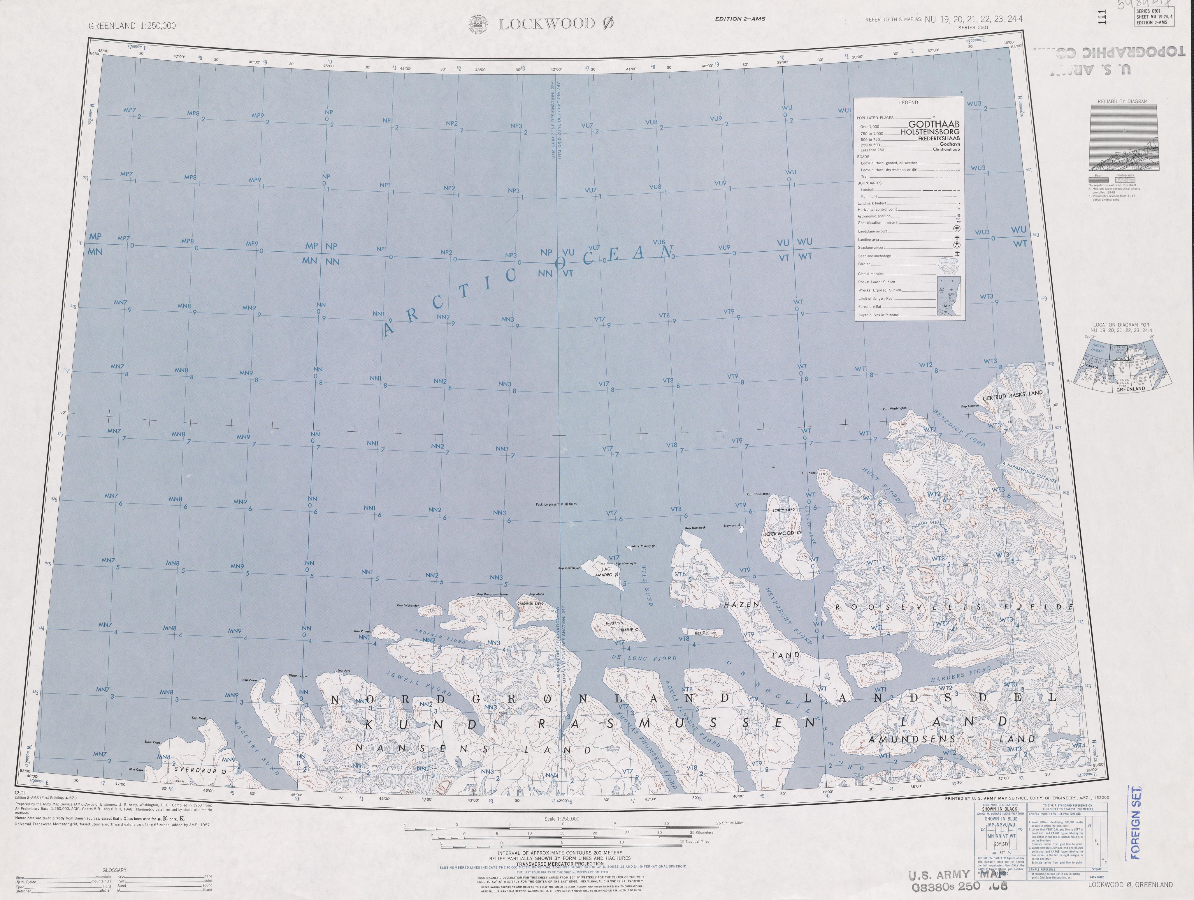
The HFIS (83.44°N, 39.10°W) is located between Kap Kane and Kap Washington in Peary Land, a part of northern Greenland. Our study site includes HFIS, Thomas Gletscher and two tributary glaciers that we informally name Glacier A and Glacier B (Fig. 1). In a 1978 orthophotograph (Korsgaard and others, Reference Korsgaard2016b; Fig. 1a) HFIS had an area of 75.8 km2; in 2020 it was 32.4 km2. The three main tributary glaciers were fronted by HFIS in 1978; in 2020, only Thomas Gletscher and part of Glacier B remain connected to the ice shelf. Mapping of the region in 1957 by the (US) Army Map Service of the Corps of Engineers (C501 Edition 2-AMS, Lockwood Ø. Quadrangle) suggests that Thomas Gletscher had a single merged outlet near the present-day northern outlet.
HFIS is characterized by several different provenance regions of ice with varying thicknesses and surface features (discussed further in Section 4.1). These unique provenance regions can affect the dynamics and flow of the ice shelf differently (Jeffries, Reference Jeffries1992). The majority of the ice shelf exhibits corrugations that are characteristic of Arctic ice shelves, but other regions are clearly derived from glacier ice and in general have a higher surface height (i.e., thicker floating ice). Sediments or cryoconite and seasonal melt ponds are also present, particularly near some of the shelf provenance boundaries where there are large amounts of accumulated rock and cryoconite debris.
Northern Greenland glaciers and fjord ice are relatively understudied compared to the Ellesmere ice shelves and other areas of Greenland. HFIS is considered to be the last remaining Arctic-style ice shelf that exists in Greenland (Higgins, Reference Higgins1988, Reference Higgins1991; Reeh, Reference Reeh, Copland and Mueller2017). Our own analysis of the 1978 photomosaic, which spans much of western Peary land, is that Hunt Fjord has the characteristics of an Arctic ice shelf, similar in many ways to the Milne and Ward Hunt ice shelves of Ellesmere Island, confirming Higgins (Reference Higgins1988) interpretation. The adjacent fjords, Conger and Benedict likely contained Arctic ice shelves in the recent past, and as of the 1978 mapping still appear to contain remnant ice-shelf areas, but the other regional inlets are generally filled with young sea ice and disaggregating glacier ice near the grounding lines. By the time of the beginning of Landsat 8 off-nadir coverage, these remnant areas (other than HFIS) were absent.
Northern Greenland has few long-term climate datasets. The closest weather station to HFIS is the Kap Morris Jessup automated weather station, ~75 km away. Several studies have investigated recent warming trends in Greenland. Westergaard-Nielsen and others (Reference Westergaard-Nielsen, Karami, Hansen, Westermann and Elberling2018) discuss the long-term seasonal temperature changes that Greenland is experiencing in different regions. In most areas, including near Hunt Fjord, mean annual air temperature has risen. Using a combination of instrumental data and ice-sheet records, Hanna and others (Reference Hanna2020) found that for the period 1991–2019 there was a significant warming trend over all of Greenland. Winter conditions warmed by 4.4°C, spring by 2.7°C and summer by 1.7°C.
3. Data and methods
3.1 Optical imagery
The 1978 airphoto mosaic was compiled by the Centre for GeoGenetics at the University of Copenhagen (Korsgaard and others, Reference Korsgaard2016a). The airphotos were rendered into a seamless 2 m mosaic of the western Peary Land region, and a sub-scene of this mosaic was used to identify ice provenance and surface texture regions on HFIS (Table 1). Assessment of early ice extent, HFIS ice provenance regions (Fig. 1a) and corrugation wavelength (Fig. 2) was determined from this image. We note that there are other datasets available that were not used in this study due to poor resolution, namely declassified satellite imagery from ARGON KH-5 Mission 9034A, from May 1962, with ~140 m resolution. The Satellite Pour l'Observation de la Terre (SPOT) images from 1988 and 1994 also indicated that ice extent and structural patterns had not changed substantially from 1978 (see Supplementary Fig. 1).
Ice thickness estimates from corrugation wavelengths adapted from Jeffries (Reference Jeffries, Copland and Mueller2017). The corrugation wavelengths measured from the 1978 image (triangles) are plotted on the linear trend line (red) from Jeffries (Reference Jeffries, Copland and Mueller2017). The cluster of black points in the lower left are MYFI thicknesses and in the upper right are Ellesmere ice shelf and ice island thicknesses reported by Jeffries (Reference Jeffries, Copland and Mueller2017). The linear equation shown in Jeffries (Reference Jeffries, Copland and Mueller2017) is modified.

HFIS extent, provenance extent and calving events, 1978–2019

Error is ±0.2 km2 of area measurements of provenance regions, ice shelf and calvings.
a Area measured at time of 1978 or Landsat image acquisition.
b Region A: MYFI, Region B: Glacier A tongue, Region C: NE Ice Shelf, Region D: Glacier B tongue, Region E: Ice shelf compression area, Region F: middle ice shelf area, Region G: Thomas Gletscher North tongue, Region H: Thomas Gletscher South tongue.
Landsat 8 Operational Land Imager (OLI) product L1GT imagery was used to assess surface characteristics of HFIS as well as to determine the ice flow speed of Glaciers A and B (Figs 1b–e). The nominal Landsat 8 coverage range is 82.4°N/S (with a nadir track of 81.5°N/S) but it has the capability to acquire off-nadir imagery, extending coverage to ~84.5°N/S. This is further north than the footprint of Sentinel 2a and b, despite the wider swath width of the Sentinel-2 system (185 km for Landsat 8; 290 km for Sentinel-2). Landsat 8 acquired off-nadir images covering both poles during their respective summer seasons in 2016, 2017, 2018 and 2020. Images were selected based on low cloud cover and then processed in QGIS software for quantitative measurements of HFIS extent changes, using bands 1, 2 and 3. Ice flow speed of northern HFIS was determined using PyCorr, a Python-based image correlation software tool (Fahnestock and others, Reference Fahnestock2016). PyCorr measures ice displacement between two images by comparing the correlation between image chips (small subscenes) extracted in a grid pattern over both images. A Landsat 8 image pair from 2017 (05 August) and 2018 (08 August) produced the best coverage of ice flow velocities of Glacier A, B and the northern edge of HFIS; this was supplemented in the south using the 2016 (17 July) image, and the speed fields were merged (and averaged where overlapping). Ice flow speed errors are a combination of geolocation errors for the image pair (typically ~5 m) and measurement errors on the individual correlations (0.1 pixel or 1.5 m; Fahnestock and others, Reference Fahnestock2016). For images separated by one year, error is ~±7.5 m a−1.
The Terra and Aqua satellites (launched in 2000 and 2003, respectively) both carry the MODIS sensor, which generates global daily coverage in 36 bands. A survey of images using NASA's Worldview web browse service (https://worldview.earthdata.nasa.gov) indicated several significant calving events in the 2012–2020 period, which we documented for date of occurrence and area. True color images, from bands 1, 3 and 4, with red-band sharpening (band 1, 250 m resolution), were used to produce images of the identified HFIS calving events.
3.2 Corrugations
A relationship between ice thickness and the wavelength of the corrugations on Arctic ice shelves was determined by Jeffries (Reference Jeffries, Copland and Mueller2017), who used ice shelf, ice island and MYFI thickness data from various studies to determine an empirical relationship between the wavelength of the corrugations and ice thickness. They used a regression analysis to obtain an empirical relationship. Since there are no known ice thickness data for HFIS, we instead used estimated wavelength values to infer ice thickness, using the empirical relationship developed by Jeffries (Reference Jeffries, Copland and Mueller2017). To estimate wavelengths on HFIS, we measured the distance between the corrugations using the QGIS tool on the 1978 photo mosaic. Evaluation transects were set perpendicular to corrugation crests in areas that had several sequential well-defined corrugations. In several regions, we used two parallel lines <100 m apart to assess variability in our assessment. Regions not included were A, and G, due to the lack of organized parallel corrugations. The crest-to-crest distance (i.e., wavelength ‘x’) was then entered into the two regression equations that were presented in Jeffries (Reference Jeffries, Copland and Mueller2017) to determine ice thickness (‘y’):


We include the results of Jeffries (Reference Jeffries, Copland and Mueller2017; see their Fig. 2.8) together with our results in Figure 2 and Table 2. We note that Eqn (1) is modified from Jeffries (Reference Jeffries, Copland and Mueller2017) to show the dependence y on x (instead of x on y as presented by Jeffries). We use these equations to calculate the approximate ice thickness of the different ice provenance regions in the 1978 orthophotograph and in the 2016 Landsat image.
Statistics of measured corrugation wavelength and derived ice thickness for HFIS provenance regions in 1978 and 2016 from 1978 orthophotographs and 2016 Landsat imagerya

a Corrugation wavelengths for each region are determined using two profile lines in each of the red boxes in Figure 1a. x̅ is the mean corrugation wavelength (m), σ is the std dev. (1 σ), H is the estimated thickness (m) from the Jeffries (Reference Jeffries, Copland and Mueller2017) equations, linear and quadratic (‘quad’).
3.3 ICESat and ICESat-2
Our study used ICESat and ICESat-2 data (Zwally and others, Reference Zwally2002, Reference Zwally, Schutz, Dimarzio and Hancock2014; Markus and others, Reference Markus2017; Smith and others, Reference Smith2020) to examine elevation changes over ~2003–2019 (i.e., the combined period covered by ICESat, 2003–2009, and ICESat-2, 2018–2019). The elevation change determination relied on slope correction of the laser altimeter tracks using the Arctic DEM. Within a grid of 200 × 200 m cells, the full-resolution (2 m postings) Arctic DEM provided local slopes so that multiple ICESat near-repeat tracks could be aligned to a single mean elevation for the cell; similarly, the ICESat-2 tracks could be adjusted for local slope in the same cell. Differencing the corrected mean cell elevations for ICESat and ICESat-2 data provided the elevation change values in cells containing data from both satellites. ICESat acquired laser altimetry profiles in a series of 8- and 31-day campaigns, providing several repeat profile measurements over the period 2003–2009. ICESat ground footprints are spaced every 172 m along the sub-satellite track, with elevation data returned from laser altimetry footprints ~60 m in diameter (Abshire and others, Reference Abshire2005). We used the data product GLAH06 version 34 for our analysis, accessed from https://nsidc.org/data/GLAH06/versions/34, which included corrections for tides and detected saturation over bright surfaces. ICESat-2 was launched in September 2018 and is equipped with photon-counting detection technology. This system uses a 532 nm laser output split into six beams, arranged in three beam pairs of one strong and one weak beam, with pairs separated by 3.3 km and has a 91-day repeat cycle. The ICESat-2 data product ATL06 provides a linear surface approximation of 40 m overlapping segments along each ground track (Smith and others, Reference Smith2019).
We used the ICESat-2 tracks to examine the vertical structure and elevation of the HFIS surface across the ice provenance regions (Fig. 3). We used the ICESat-2 ATL06 Version 3 Revision 1 data product, which has no tidal correction applied. In this region, the tidal range is ~0.5 m (Padman and others, Reference Padman, Siegfried and Fricker2018). Only the strong beam returns were used for this analysis, as we sought information on elevation change and not local slope (the strong–weak beam pairs are separated by 90 m for measuring local cross-track slope). Track acquisitions from October and November 2019 crossing HFIS were used. ICESat-2 vertical errors are less than a decimeter, similar to ICESat (Brunt and others, Reference Brunt, Neumann and Smith2019). October–November acquisitions of tracks 276 GT1R, 407 GT3R, 468 GT1R and GT2R, and 779 GT2R provided detailed information on ice height and by inference ice thickness for most of the ice provenance regions of HFIS, where GT is ‘ground track’ and L/R is ‘left/right’.
Left: ICESat-2 tracks from 2018 plotted over the 08 August 2018 Landsat 8 image with provenance regions (yellow dashed lines). Right: ICESat-2 annotated profiles showing the topography of the ice shelf and the provenance regions. GA and GB refer to unnamed Glacier ‘A’ and ‘B’ respectively.

3.4 DEMs
The 1978 stereo airphoto DEM was obtained from the dataset described in Korsgaard and others (Reference Korsgaard2016a). The DEM was produced by using stereophotogrammetry controlled by field surveyed geodetic ground control points and is referenced to the WGS84 ellipsoid. The product is gridded at 25 m ground-equivalent scale, with an accuracy of 10 m horizontally and 6 m vertically, and a precision of <4 m (Korsgaard and others, Reference Korsgaard2016a). Vertical error is dominated by variations in the steep mountain terrain adjacent to glaciers and floating ice. Aerial photographs were acquired on 23 July 1978 (Bjørk A., personal communication).
A second DEM used in our study, the ArcticDEM from the Polar Geospatial Center (PGC) was generated from stereo panchromatic band satellite images from WorldView-1, WorldView-2, WorldView-3 and GeoEye-1 (Morin and others, Reference Morin2016; Porter and others, Reference Porter2018; https://www.pgc.umn.edu/data/arcticdem). These were used to create 2 m resolution DEM strips for all land North of 60°N. We used the gridded Arctic-wide mosaic product, which is compiled from many strips that have undergone co-registration, blending and feathering. The total shift in the ArcticDEM mosaic once registered to ICESat is 4.62 m for our study area gridcell (Glennie, Reference Glennie2018). In the HFIS region, images used for the DEMs were acquired between April 2012 and April 2017, with the best quality strips (low cloud cover, smooth DEM rendering) acquired on 21 April and 27 April 2013, 11 May 2014, 01 June 2015 and 26 April 2016; i.e., the main contributing strips were from late spring. For our study we re-projected the DEMs into Arctic Polar Stereographic/WGS84 projection (EPSG: 3995) and resampled the ArcticDEM in the Hunt Fjord region to 25 m ground-equivalent gridcell size to match the gridding of the 1978 DEM.
We assessed the 1978 DEM for bias relative to the ArcticDEM, assuming that the latter was more accurate vertically. We adjusted the elevations in the 1978 DEM so that the weighted (by area) difference was zero in seven well-lit ice-free fjord wall regions adjacent to the HFIS (Supplementary Fig. 2). We applied a reliability masking to the 1978 DEM as suggested by Korsgaard and others (Reference Korsgaard2016a). The overall bias of the 1978 DEM in the Hunt Fjord region using this method was −2.97 ± 2.36 m (i.e., low relative to the ArcticDEM). The std dev. of the differenced elevations in smooth surface areas adjacent to Hunt Fjord (upper glacier catchments, low-slope land areas) was ±0.5–2.2 m. This adjustment to the 1978 DEM supported an approximate evaluation of ice-shelf elevation change over HFIS and the grounding zone of the glaciers in the period 1978–2015.
We extracted profiles from the two DEMs along the ICESat-2 track sections shown in Figure 3 to create an assessment of ice-shelf elevation changes over the ice provenance regions between 1978 and ~2015 (the mean date of the ArcticDEM in our region). The profiles are shown in Figure 4. We also subtracted the 1978 DEM from the ArcticDEM over the entire HFIS study area to assess the elevation changes of the HFIS and the lower reaches and grounding zones of the surrounding tributary glaciers.

Elevation changes between the ICESat and early ICESat-2 operational periods were evaluated using the ArcticDEM to interpolate between the two groundtrack patterns. ICEsat data were averaged from 2003 to 2009 with a midpoint in 2006 and ICESat-2 data were averaged from October 2018 to July 2020 with a midpoint in 2019. The Arctic DEM provided a slope correction for the ICESat and ICESat-2 track data in 200 × 200 m grid cells. Using the full-resolution Arctic DEM (2 m) the multiple ICESat and ICESat-2 passes were adjusted for local slopes, providing a mean reference elevation for the ~2006 timeframe (ICESat) and 2019 timeframe (ICESat-2). Cells that contain both ICESat and ICESat-2 tracks can provide a slope-corrected mean elevation change for the period spanning the two satellite missions. This gives a total elevation change in meters with an error of decimeters for flat areas.
3.5 Ice-shelf thickness and area, provenance regions and retreat events
For our study, initial ice-shelf area, ice provenance regions and shelf extent were determined using the 1978 orthophotograph (Fig. 1a). The ice-shelf provenance areas were re-examined and boundaries were revised slightly using the 2016 Landsat 8 image (Path 040, Row 245, 17 July 2016), with changes interpreted as being largely due to tributary glacier flow against relatively slow-moving MYFI areas. For 1978, the extent of the provenance regions was determined using the orthophotograph in conjunction with the 1978 DEM to assess the areas that were MYFI versus glacier lobe ice in the ice shelf. Regions and frontal positions were outlined at least three times and then adjusted for consistency. Boundaries were identified based on corrugation orientation and linearity, and to a lesser extent on ice-shelf elevation. Estimated regional areas have an uncertainty of ±0.2 km2, based on repeat mappings performed by the same individual, due to the ambiguity of the boundaries.
To estimate the ice-shelf thickness using elevations from ICESat-2 and the DEMs we used the following equation:

where H is the thickness of the ice shelf, h is the height of the floating ice (corrected for the EGM2008 geoid), ρ w is the density of seawater, and ρ i is the density of the ice. We assume the density of the sea water to be 1028 kg m−3 and the ice to be 900 kg m−3 as studies on the Ward Hunt Ice Shelf suggest (Ragle and others, Reference Ragle, Blair and Persson1964; Jeffries and others, Reference Jeffries, Sackinger, Krouse and Serson1988; Braun, Reference Braun, Copland and Mueller2017). With extensive surface melting every spring and summer, and surface ponding, we assume any firn layer is heavily densified by refrozen meltwater.
We evaluated the grounding line retreat of the four tributary glaciers. The grounding line was determined using the ArcticDEM and 1978 DEM, using the elevation to calculate the slope using the GIS raster slope calculator and selecting the downstream boundary where surface slope had a sudden drop below ~3°; optical images were used to help inform the location of the grounding line by identifying changes in the surface features. For the ArcticDEM and 1978 DEM, 58 elevation points crossing the approximate glacier centerline along the grounding line were extracted using QGIS. Both DEMs were corrected to the EGM2008 geoid (Pavlis and others, 2012) by subtracting 26.4 m (variation of the geoid at two different points in the study area was <0.01 m), and the 1978 DEM was bias-adjusted by −2.97 m, as noted above (see Supplementary Information), giving elevations above sea level. The 58 points along the centerline of the grounding line were averaged to determine the mean grounding line elevation at the center of the glacier outlet. Error for these calculations was estimated by using the standard error of the mean. Using Eqn (3) the ice-shelf thickness was then determined using the elevation and error estimates.
3.6 Passive microwave data (SSM/I-SSMIS)
In considering possible climate-related causes for the recent increase in major calving events of HFIS, we examined regional trends in ice-sheet surface melt days on the ice sheet adjacent to HFIS to the south, and sea-ice concentration trends in the Arctic Ocean north of Hunt Fjord using passive microwave data. Both local sea-ice concentration variations and trends in total annual ice-sheet melt days were estimated using two passive microwave-based datasets. The data are from the NASA-produced Sea Ice Concentrations from Nimbus-7 SMMR and DMSP SSM/I Passive Microwave Data dataset (https://nsidc.org/data/nsidc-0051), which uses the GSFC Bootstrap algorithm Version 3.1 (Comiso, Reference Comiso2017). We used an average of the daily passive microwave-derived sea-ice concentrations for a 3 grid-cell area (each cell represents 25 km × 25 km) in the region immediately north of HFIS and the Greenland coast, available every other day from 1978 to 1987 and daily from 1988 to 2020. For determining annual total ice-sheet melt days, we averaged six 25 km grid cells, including one on Hans Tausen Ice Cap in a region south of HFIS. HFIS itself is too small for an accurate melt day determination using these data (Mote and Anderson, Reference Mote and Anderson1995; Mote, Reference Mote2007; see also https://nsidc.org/greenland-today/).
4 Results
4.1 Ice shelf provenance regions
We mapped eight ice provenance regions in the HFIS with distinct corrugation textures, surface features and relationships to adjacent glaciers and rocky debris strands on the 1978 orthophotograph (Fig. 1a). These regions are still perceptibly evolving in extent and characteristics in the 2016 and later Landsat 8 images (Figs 1b–e). As part of ongoing calving and retreat, many of these regions have lost some or all of their area over the last decade (Table 1). In our evaluation of the provenance boundaries, we considered the elevation and inferred ice thickness from the corrugation wavelengths (Fig. 2) and ice elevation profiles from ICESat-2 and the two DEMs (Figs 3 and 4).
HFIS is formed from glacier ice outflow and long-term MYFI. In 1978, Glacier A, Glacier B and Thomas Gletscher all contribute to the area of HFIS as floating ice tongues within the shelf (Fig. 1a; regions B, D, G and H). As these floating glacier tongues extend into the fjord, they thin and appear to acquire some characteristics of the MYFI elements that make up HFIS, e.g., parallel corrugations that trap meltwater ponds in summer and generally have low elevation. At the edges of the glacier tongue regions there is often a zone of increased debris cover. However, Region B, formed by the glacier tongue of Glacier A, has few of these features and extends more or less directly toward the mouth of the fjord. Regions D, G and H formed by outflow from Glacier B, the northern outlet of Thomas Gletscher, and southern outlet of Thomas Gletscher, respectively, possess parallel corrugations and have clear indications of flow in the form of streaklines. Moreover, the image series shows these features are moving due to continued spreading of the ice tongue areas and outlet glacier flow. Region D has rifts northeast of the grounding line that have shifted with flow over the years. In the 2020 Landsat image, a new fracture has formed near the grounding line in Region D (Fig. 1e).
Regions A, C, E and F are interpreted as corrugated multi-year fast ice but have distinct corrugation patterns. Regions A and C have linear parallel corrugations with shorter wavelengths. Unlike Region A, Region C also contains thicker embedded ice areas. These are pieces calved from the thicker part of the ice shelf or the glacier-sourced ice of Region B, and resemble ‘sikussak’, a composite of landfast sea ice and icebergs typical of Greenland fjords and areas of the Ellesmere ice shelves (Dowdeswell and Jeffries, Reference Dowdeswell, Jeffries, Copland and Mueller2017).
Three regions do not have clear indications of land ice origins. Region E is adjacent to the east fjord wall and contains parallel corrugations with many meltwater ponds in the 1978 image. The corrugations run parallel to the fjord wall, unlike the corrugations in Region D that are more variable. Region E appears to be compressed folded ice, likely originating from multi-year landfast ice or possibly a detached area from an older glacier ice tongue. We interpret Region F as a ‘compressive strain confluence area’ because it lies between thicker glacier tongue ice from both Region D and Region G. The corrugations in Region F are distinct but chaotic and lack any clear pattern. We note a clear range of ice thicknesses in Region F, the thick strain confluence area and the thin strain confluence area, as measured in ICESat-2 data (Fig. 3). Region H, at the southern end of the HFIS, between the northern and southern outflow areas of Thomas Gletscher, appears to be similar to Region F, a compressive strain confluence area, but has slightly longer wavelengths in its corrugations that are more similar to Region B (Table 2). Distance corrugations are not distinguishable in the Landsat imagery in Region H but may still be present.
The ice regions have different ice flow speeds estimated in this study (2016–2018) (Fig. 1c). Region E is relatively stagnant, whereas Region D has flow speeds up to 30.2 m a−1, while Region F has a slower flow speed of 6.1 m a−1. The tributary glaciers had generally high flow speeds as well with Glacier A at 24.5 m a−1, Glacier B at 14.6 m a−1 and Thomas Gletscher at 23.7 m a−1. The ice flow speed is likely contingent upon ice thickness, ice strain from interaction with glacier flow and fjord walls, and indirectly contingent upon ice origin.
4.2 Ice thickness, ice thickness change and structural change since 1978
4.2.1 Provenance regions ice thicknesses
Determining the ice thickness of the ice shelf and its provenance regions is difficult without in situ measurements because the ice is relatively thin. In this section, we use several methods to estimate ice thickness. Following Jeffries (Reference Jeffries, Copland and Mueller2017) two equations (linear and quadratic) were determined to relate corrugation wavelength to ice thickness. When applied to our measurements of corrugation wavelength (Fig. 2), we find that regional ice thickness varied significantly, from 4 to 32 m. Applying both equations from Jeffries (Reference Jeffries, Copland and Mueller2017) to our measurements of corrugation wavelength (Fig. 2) indicated that ice thicknesses vary significantly, from 4 to 32 m. This is within the range of ice thicknesses reported for MYFI and the Ellesmere Ice Shelf ice and ice islands (Jeffries, Reference Jeffries, Copland and Mueller2017).
The different ice-shelf regions have distinct ice elevation ranges, and by inference using Eqn (3), ice thicknesses. Ice-shelf provenance region elevations retrieved from ICESat-2 range from very low-freeboard ice (nearly indistinguishable from the thinnest sea ice, see Track 779 in Fig. 3b), to between 6 and 8 m of freeboard in the glacier lobe regions (Regions D and G, Fig. 3b Tracks 779 and 468 GT2R and GT1R), and over 8 m on the lowest grounded ice of Thomas Gletscher (Fig. 3b Track 276). Region F, the unknown-provenance region, is also thicker than sea ice, with 2–4 m freeboard (Fig. 3b Track 407). The corrugations are evident in the ICESat-2 data in several regions (Fig. 3), with 1–3 m amplitudes. For the shorter wavelength corrugation areas (Regions E and F) the corrugation structure is undersampled, therefore we did not calculate ice thickness from the corrugations detected by ICESat-2.
Our three methods (corrugation wavelength correlation, ICESat-2 and DEMs) for measuring the surface height of the various provenance regions report similar ice thickness values. Some HFIS provenance regions are thinner than other Arctic ice shelves and ice islands yet are thicker than the MYFI components of those features (Jeffries, Reference Jeffries, Copland and Mueller2017). We note that our assessment area for region D, the Glacier B-sourced ice tongue, was not near its grounding line, where it would likely have been thicker. This area, particularly the southern portion of the lobe, has less distinct corrugations.
4.2.2 Ice thickness and structural changes
The structure and thickness of the HFIS provenance regions and tributary glaciers have changed over time. We used the ICESAT-2 nominal track locations to investigate elevation profiles from the ArcticDEM and 1978 DEM (Fig. 4). While noise in the 1978 DEM is large, a running-mean smoothing at 250 m scale (averaging 10 measurements from the 1978 DEM) provides a ~±1 m accuracy profile (assuming the errors are random at ±4 m in the 25 m DEM). The comparison indicates in a semi-quantitative way how the regions have changed in freeboard and thickness over time. Most notably, there has been a significant decrease in freeboard elevation in Region D (outflow glacier lobe of Glacier B), with some areas decreasing by ~40% (3.5 m) resulting in an inferred ice thickness decrease on the order of ~30 m. The thickening in Region E is also evident, increasing from ~1 m freeboard to just under ~4 m as measured in the Arctic DEM.
All the tributary glaciers show substantial elevation loss at and upstream of their grounding zone regions inferred by distinct slope breaks relative to the ice-shelf surface seen in the DEMs (Fig. 5). Centerline ice-shelf thicknesses were determined using Eqn (3), coordinates of the end points for the grounding line central portions are in the Supplementary Table S1. The cross-sectional profile lines (red lines in Fig. 5) were chosen as the along-flow area with the greatest amount of retreat, independent of thinning. Glacier A has retreated and thinned by a marginal amount (<13 m thinning), whereas Glacier B and both outlets of Thomas Gletscher have experienced significant changes (Table 3), with centerline ice-shelf thinning of up to 61 m and grounding line retreat up to 480 m. As of 1978, the grounding line of the southern outlet of Thomas Gletscher appears to have retreated ~5 km further south (near the southern edge of the area shown in Fig. 1a) when compared to the 1957 map, though the methods of grounding line determination in 1957 are unknown.
Grounding lines of the HFIS tributary glaciers determined by the break in slope (to <0.05°). Profile elevations across the grounding zone are relative to the EGM2008 geoid representing sea level. Zero indicates which position starts of the cross-sectional profile lines shown in the map view. The black points indicate the sections of the grounding lines that were used for ice thickness calculations (Table 3). The background images are shaded relief subscenes of the 1978 DEM, 2.5 km on a side, with locations indicated in Figure 6.

Tributary glacier grounding line changes: elevation, thickness and retreat

Ice shelf thicknesses were calculated using Eqn (3).
a Elevation change at the intersection of the centerline and 2015 grounding line.
b Measured along the central portion of the grounding lines (see Supplementary Information).
Figure 6a is a map of the difference between the ArcticDEM (average acquisition year for HFIS area is ~2015) and the 1978 stereo airphoto-derived DEM. Overall, surface elevation on HFIS declined over this 37-year period. We note that the 1978 orthophotographs and DEM are compiled from stereo aerial photographs acquired on 23 July and thus reflect late summer conditions (and there are abundant melt ponds in the images), while the ArcticDEM component image strips in this area are almost entirely from mid- to late-spring (2013–2016). We therefore infer that the Arctic DEM likely had a thicker snow cover.
(a) Difference of ArcticDEM and1978 stereo airphoto-derived DEM of the HFIS region. A bias in the 1978 DEM of 3.0 ± 2.4 was removed, see Supplementary Information. High variation (noise) in the thin snow and rock areas of the DEM difference is due in part to poor elevation quality in the 1978 DEM rendering. However, we note that the ice surfaces have far less short-scale variation. Yellow boxes are 2.5 km cells used for groundling line analysis (Fig. 5). (b) Difference of gridded ICESat-2 elevations (from ICESat-2 tracks acquired in 2019) and ICESat elevations along ICESat tracks. ICESat-2 track data were extrapolated to a near-continuous grid using the ArcticDEM as a guide. Repeat ICEsat tracks were slope-corrected using the ArcticDEM slopes. The ICESat–ICESat-2 differenced grid cells are overlain on a shaded relief image of the ArcticDEM of the HFIS study regions.

Our results show a range of ice elevation changes between 1978 and 2015. Region E experienced significant elevation increases (Fig. 4d), likely from additional deformation and thickening of the ice from the compressive stress exerted from the expansion of the Glacier B tongue, represented by Region D. However, other areas of the ice shelf experienced elevation loss, such as Region D in the area near the grounding line of Glacier B. Region G has a mixed pattern of very slight elevation decline in the northern portion of the Thomas Gletscher ice tongue but with some elevation increase in the southern section. We interpret the elevation increase to be a result of compression and thickening of the ice due to inflow from Thomas Gletscher South, similar to Region E. Region H, at the far southern end of the HFIS, shows a mixed pattern, probably indicating near-zero net change but with some horizontal motion of the corrugated surface.
These general patterns are also evident in Figure 6b, which shows the ICESat to ICESat-2 differences from ~2019 to ~2005. While the data are sparser in Figure 6b than Figure 6a, the patterns of significant elevation loss on the glacier tributaries, and near-zero to slight loss over most of the ice shelf (Fig. 6a), confirm the general pattern of change from the DEM differencing.
Regions A, B and C calved from HFIS beginning in 2012 and in subsequent events (Figs 1b–d, 7; Table 1). Regions D and E lost substantial fractions of their areas in calving events beginning in 2019 (Figs 1d, e, 7e, f; Table 1). Figures 7a and b display the break-up event in 2012 that resulted in an area loss of 8.9 ± 0.2 km2. In 2016 another break-up event occurred (Figs 1b, 7c, d; Table 1), reducing HFIS by a further 21.1 ± 0.2 km2. In 2017 and 2018 the ice shelf had landfast sea ice at the front of the fjord, possibly protecting the ice shelf from further break-up. In 2019, another 12.5 ± 0.2 km2 broke away overnight on 26–27 of July (Figs 7e, f).
MODIS images of 2012, 2016 and 2019 calving events illustrating connection with limited landfast fast ice loss.

These break-up events result in a total reduction of 42.5 km2 (~56%) relative to the 1978 extent of HFIS. In addition to the area changes, the corrugations shifted in orientation by several degrees (northern Region D, 9 degrees, 1978–2016; Region E, 7 degrees) and the glacier lobes in Regions D and G have evolved, appearing to have spread out more into HFIS, and displacing the adjacent areas of Region F.
5. Discussion
HFIS is one of the last Arctic-style ice shelves remaining. Its remote, rarely visited location has kept it from previous detailed study, and yet its complex structure and recent retreat make it an informative example of how Arctic ice shelves have responded to intense regional climate warming over the past few decades. HFIS has undergone significant changes since 1978, including several recent break-up events, thinning and the tributary glaciers that feed HFIS have also thinned and likely sped up. A further look at the regional conditions during the break-up events provides insight into the causes of Arctic ice-shelf retreat, as developed below.
HFIS formed sometime well before 1978, probably by at least several decades but perhaps up to a few centuries before, as inferred from the complex interaction and deformation structures of what we interpret as land- and ocean-derived ice regions. Assuming the conditions of formation are similar to the Ellesmere ice shelves, then it is possible it formed 4000 years ago (Vincent and others, Reference Vincent, Gibson and Jeffries2001). Like several Ellesmere ice shelves, HFIS is formed from a combination of glacier ice and MYFI. The different origins of ice contribute to HFIS's dynamic nature, with varying surface characteristics and ice thicknesses. The continuing, but very slow, changes in the extent of the provenance regions (Table 1), and the very slow expansion of the glacier tongues, are consistent with the inference that the HFIS is at least hundreds of years old.
Unlike the Ellesmere Arctic ice shelves, HFIS was generally stable during the period 1978–2012, having no substantial change in extent at the level of MODIS resolution. The identified HFIS provenance regions experienced only minor area changes since 1978 as the ice continued to move and evolve. However, since 2012, calving of the HFIS northern edge has been significant, calving a total of 33.6 km2, or 45% of its 1978 extent, between 2012 and 2020.
For comparison, the once-large Ellesmere Ice Shelf fringe (estimated at 9000 km2 by Peary, Reference Peary1907) lost 90% of its area between 1906 and 1982, with significant loss by the 1950s, leaving only the individual fjord-based ice shelves. These remained relatively stable through the late 1980s and 1990s but then began a period of rapid retreat coincident with intense regional climate warming (Copland and others, Reference Copland, Mueller and Weir2007). The Ward Hunt Ice Shelf split into two sections between 2000 and 2002 (Braun, Reference Braun, Copland and Mueller2017) and in 2008 lost 22 km2 (England and others, Reference England2008); Ayles ice shelf lost 99% of its area in 2005 (Copland and others, Reference Copland, Mueller and Weir2007), and Serson lost 64% of its ice extent in 2008 (Mueller and others, Reference Mueller, Copland, Jeffries, Copland and Mueller2017).
The demise of the Ellesmere Arctic ice shelves is attributed to warming air and ocean temperatures, loss of a consistent landfast sea-ice fringe (i.e., more open water periods at the shelf ice front) and wind events. Warming air temperatures can increase surface melting and can lead to weakening of the ice shelf, with potential calving events through hydrofracturing. The warming ocean can increase basal melt causing thinning and therefore weakening. The loss of landfast sea ice can contribute to ice-shelf weakening and subsequent collapse by a number of effects: (a) loss of buttressing, that otherwise provides resisting stress, inhibiting ice-shelf rifting and calving (Cassotto and others, Reference Cassotto, Fahnestock, Amundson, Truffer and Joughin2015; Bendtsen and others, Reference Bendtsen2017); (b) loss of protection from long-period wave-driven flexure (Reeh and others, Reference Reeh, Thomsen, Higgins and Weidick2001; Copeland and others, Reference Copland, Mueller and Weir2007; White and others, Reference White, Copland, Mueller and Van Wychen2015; Massom and others, Reference Massom2018); and (c) greater open water exposure that significantly affects the local energy budget, substantially increasing both the surface and sub-surface ice melt rates. An example of the latter, Bendtsen and others (Reference Bendtsen2017) found that during open water periods at the Flade Isblink Ice Cap glaciers surface melt in August increased to ~10 m month−1 from ~0.5 m month−1. Wind events, including föhn events, have been known to increase surface melt significantly and potentially trigger ice-shelf collapse events in the Arctic and Antarctic (Copland and others, Reference Copland, Mueller and Weir2007; Turton and others, Reference Turton, Kirchgaessner, Ross, King and Kuipers Munneke2020).
The HFIS appears to have thinned prior to the observed break-up events in its thickest areas, but the thinner provenance shows both minor thickening and thinning, based on the indications of surface elevation change between 1978 and 2019 (the time elapsed between the two DEMs; Figs 4 and 6a). Regions D, F and parts of H have likely thinned by several meters between the time of the two DEMs. In contrast, during the same interval Region E thickened (Figs 4 and 6a), although the trend in elevation for this region from the two altimetry satellites is not determined (Fig. 6b). Additionally, the corrugations of Region E have rotated in a manner consistent with increased compressive stress from the glacier lobe of Region D, likely arising from increased outflow of the Glacier B tributary. The observed increase in elevation for Regions E and G are not explainable by tidal height differences (given the tidal range is only ~0.5 m in Northern Greenland; Padman and others, Reference Padman, Siegfried and Fricker2018). The thickening is also unlikely to be due to basal accretion, given the thickness of the shelf (tens of meters). Basal accretion on floating ice layers due to cold air temperatures, e.g., winter weather, is very slow once ice thicknesses exceed ~2 m (Ebert and Curry, Reference Ebert and Curry1993). If there were supercooled waters flowing beneath the ice shelves, basal accretion would be possible; however, oceanographic data do not support this hypothesis (Bendtsen and others, Reference Bendtsen2017; White and Copland, Reference White and Copland2019).
The tributary glaciers have all decreased in ice thickness by several meters, particularly in the areas immediately above their estimated grounding lines. Three of the four glaciers we evaluated show significant grounding line retreat since 1978. Glacier A shows a nearly stationary grounding line position, but also a relatively small elevation change, on the order of several meters over the glacier trunk (Figs 4–6). Ice speed changes are also consistent with these observations: Glacier A shows no change in speed since the earlier study (1963–1978; Higgins, Reference Higgins1988, Reference Higgins1991; Fig. 1c), while Glacier B shows ice speed increases of 6.6 m a−1 noting however that errors in our flow speed measurement are large compared with the observed change (±7 m a−1).
Few factors have likely contributed to the observed glacier ice thinning, including surface meltwater runoff, drainage within the ice shelf or basal melting. In adjacent fjords in northern Greenland (Sherard Osborn Fjord, the outlet area for Ryder Glacier and Petermann Fjord containing Petermann Glacier), Atlantic Water (AW) at up to +0.3°C (at 500 m) underlies cold Polar Water (−1.5°C, and low salinity, <34 g L−1) beginning at ~60 m depth (Münchow and others, Reference Münchow, Padman, Washam and Nicholls2016; Jakobsson and others, Reference Jakobsson2020, their Fig. 2). Ocean water temperatures there have a steep thermal gradient below 60 m, warming to −0.5°C by 150 m depth. Additionally, warm AW has been found recently in Greenland fjords all around the island, driving increased glacier melting (Joughin and others, Reference Joughin, Alley and Holland2012; Straneo and others, Reference Straneo2012; Straneo and Heimbach, Reference Straneo and Heimbach2013). At Yelverton Bay in northeastern Ellesmere Island, using TOPAZ4 Arctic Ocean Reanalysis data, White and Copland (Reference White and Copland2019) found the highest increase in ocean temperatures occurred between 2006 and 2010, warming by up to 1.07°C at a depth of 100 m.
We infer that the large elevation decline we see at and immediately upstream of the grounding lines for the tributary glaciers (the regions of thicker ice) is due to basal ice erosion at the grounding line. We attribute this to the likely increased presence of AW in Hunt Fjord at depths below 60 m, similar to Ryder Glacier and Petermann Fjord. We estimate that the base of glacier ice extended below 60 m for all four tributary glaciers in 1978 (Table 3); however, by 2015, only the southern Thomas Gletscher outlet (south end of Region H) had an estimated ice draft >60 m.
According to previous studies, one of the main contributing factors for ice-shelf break-up is a change in the presence of landfast sea ice (e.g., Massom and others, Reference Massom2018). We examined the sea-ice concentration record derived from a series of satellite-borne passive microwave sensors (see https://nsidc.org/data/nsidc-0051) to look at the changing sea-ice concentration for 1979–2020 (Fig. 8a). The record shows that low-concentration and open-water periods occurred near Hunt Fjord many times in the 1979–2020 period, both before and after MODIS data show calving events beginning in 2012. There is a reported relationship between off-shore wind events and the break-up of ice shelves, involving the removal of landfast ice, followed by increased wave action (Copland and others, Reference Copland, Mueller and Weir2007; White and others, Reference White, Copland, Mueller and Van Wychen2015). The MODIS imagery indicates that break-up events occur during periods when fast ice is removed; however calving events do not always occur when MYFI is absent.
(a) Daily passive microwave-derived sea-ice concentrations, 1979–2020, of a region immediately north of Hunt Fjord and the Greenland coast (as indicated by the blue square in the inset map), average of three 25 km grid cells from NSIDC's NASA-produced Sea Ice Concentrations from Nimbus-7 SMMR and DMSP SSM/I-SSMIS, using the GSFC Bootstrap algorithm Version 3.1 (Comiso, Reference Comiso2017). (b) Annual total surface ice-sheet melt days, 1979–2020, from passive microwave determination for the northernmost region of the Greenland Ice Sheet (as indicated by the blue squares in the inset map), average of six 25 km grid cells, including one on Hans Tausen Ice Cap (Mote and Anderson, Reference Mote and Anderson1995; Mote and others, Reference Mote2007; see also https://nsidc.org/greenland-today/). Black lines and areas mark the end-of-season annual area losses (±1 km2) for the HFIS. No losses were evident in MODIS images early in the summer of 2012 relative to the 1978 orthophotograph.

Surface melting over the same period (1978–2020; Fig. 8b) shows that northern Greenland has experienced a doubling in the number of melt days (Fig. 8b) between the 1980s and the 2010s. The record surface melt season in 2012 for the ice-sheet region closest to HFIS was triple the melt days of the earlier years in the record. White and others (Reference White, Copland, Mueller and Van Wychen2015) found the recent break-ups in other Arctic ice shelves are also correlated with the highest number of melt days on record. This coincides with recent temperature trends for Greenland and the Arctic, where mean annual temperatures have increased by several degrees, in some regions as much as a 6–7° increase (Westergaard-Nielsen and others, Reference Westergaard-Nielsen, Karami, Hansen, Westermann and Elberling2018; Hanna and others, Reference Hanna2020). Increased surface melting can fill crevasses and induce hydrofracturing events that can lead to the demise of Arctic and Antarctic ice shelves (MacAyeal and others, Reference MacAyeal, Scambos, Hulbe and Fahnestock2003; Scambos and others, Reference Scambos2009; White and others, Reference White, Copland, Mueller and Van Wychen2015). This implies that significant surface melting is a key factor in the collapse of HFIS and other ice shelves.
Sea-ice drift and compression along the northern Greenland coast has contributed further to the mechanical failure of HFIS in the period since major calvings began (after 2012). Figure 9 shows the evolution of HFIS using Landsat image subscenes highlighting distinct features that underwent deformation or fracture after calving events along the HFIS northern edge. The post-calving ice front is irregular in shape. This change may distribute stresses unevenly across the shelf front. The compression-related events (fracturing and shifting of region boundaries) appear to have occurred in the intervening fall and winter seasons between the off-nadir images. Several areas of the ice shelf experienced a southward compression, changing the orientation of the glacier tongues and lobes. Both Glacier A and Glacier B fractured at the grounding line from a right-lateral shearing force. Provenance regions B, D and E moved southward, by up to 550 m, and in the latter cases compressed and fractured parts of Region F. This compression and the new fractures contribute to the weakening of the ice shelf.
Image pairs showing structural changes at HFIS indicative of compression from the north following the major ice shelf calving that occurred in 2016. Dark red arrows highlight areas of change. (a) Glacier A developed new fractures across the grounding line with southward motion and rotation of the floating ice front in 2017. (b) South of Glacier A, parts of the ice shelf have been forced southwest. (c) Glacier B developed new fractures across the width of the glacier near the grounding line. (d) North of Thomas Gletscher, Region F moved southward after 2018. (e) Glacier B lobe (Region D) was pushed further south and west after 2018. Pale red highlight line outlines the approximate southern edge of the glacier lobe in e1 and e2 subscenes (subscenes are the same geographic area).

Patterns of Arctic sea-ice drift show that the north coasts of Greenland and the northern Canadian Archipelago experience strong compression due to the Beaufort Gyre circulation of the ice pack (Serreze and Barry, Reference Serreze and Barry2005). The thickest sea ice is 3–5 m thick off the north coast of Greenland and Ellesmere Island (Tilling and others, Reference Tilling, Ridout and Shepherd2018). During late fall, winter and spring periods, this Arctic sea ice presses into Hunt Fjord and adjacent areas. We infer that calving of the HFIS ice front has changed how these sea-ice-driven stresses are distributed within the shelf, leading to new fractures and movement of the provenance regions. HFIS did not experience obvious internal structural damage until 2016 (Fig. 9). The structural changes evident in Figure 9 are consistent with a force pushing the ice shelf southward, and not from increased outflow speed of the tributary glaciers. Therefore, we infer that this is due to sea-ice compression of the HFIS, a result of the loss of the buffer of fast ice regions of HFIS in the years before.
6. Conclusion
HFIS is an Arctic-style ice shelf that has a complex structure and varied provenances that is still evolving. HFIS has undergone changes since 1978 resulting in the thinning of the ice shelf and tributary glaciers, potential changes in ice flow speed, and a series of break-up events that has caused the area to be reduced by 56%. HFIS is similar to the Ellesmere ice shelves in composition, formation and characteristics yet was stable until the 2012 record-breaking year of ice-sheet melt days. The analysis of the Landsat and MODIS imagery and passive microwave data indicates that HFIS calving events coincide with the absence of MYFI, yet despite several seasons when MYFI was absent prior to 2012, calving events did not occur. Mechanically induced fracturing from sea-ice forces likely preconditioned the ice shelf to disaggregation by weakening the structural integrity allowing it to calve more easily. Calving only initiated when melt days increased, which more than doubled after 2010 relative to the late 1970s and early 1980s. This almost certainly led to thinning and weakening of the ice shelf, with longer summer periods of extensive melt ponding increasing the potential for hydrofracture (Scambos and others, Reference Scambos2009). Ice-shelf weaknesses were likely exacerbated by the influence of AW, melting the base of the ice shelf and in particular the regions of the thickest floating ice.
A further destabilizing effect of thinning and subsequent summertime calving is a susceptibility to ice-shelf compression and damage from the Arctic winter pack. The evidence from satellite images along with the timing of the damaging events imply that the loss of the outer parts of the ice shelf, and perhaps basal thinning, reduced the durability of the HFIS with respect to sea-ice compression.
We anticipate further retreat of HFIS in this decade due to the ice shelf's sensitivity to climate change, and to the structural fracturing and weakening that has already occurred. As HFIS continues to break-up there will likely be a significant loss of buttressing to the tributary glaciers. With increased heat gain in the ocean, longer open water periods and increased surface melt days, the glaciers in the Hunt Fjord region will likely continue to retreat. This has been noticed elsewhere: the removal of glacier tongues and ice shelves is causing rapid disintegration of the surrounding glaciers.
Supplementary material
The supplementary material for this article can be found at https://doi.org/10.1017/jog.2022.44
Data
The off-nadir Landsat 8 images are available from the USGS EarthExplorer website at https://earthexplorer.usgs.gov. Our access to MODIS imagery of calving events and local fast ice conditions came from NASA's Worldview website at https://worldview.earthdata.nasa.gov. The orthophotographs and derived DEM for northern Greenland are thoroughly described in Korsgaard and others (Reference Korsgaard2016a) and are available at http://dx.doi.org/10.7289/V56Q1V72. ICESat and ICESat-2 data were accessed at the National Snow and Ice Data Center at https://nsidc.org/data/GLAH06/ versions/34 and https://nsidc.org/data/atl03. NSIDC was also the source of both the sea-ice concentration data (https://nsidc.org/data/nsidc-0079) and the Greenland ice-sheet surface melt days data (available from NSIDC upon request, based on http://nsidc.org/data/nsidc-0080.html; see also https://nsidc.org/greenland-today/about-the-data/). The C501 Edition 2-AMS, Lockwood Ø. Quadrangle Map was obtained from the Polar Geospatial Center at https://data.pgc.umn.edu/maps/arctic/nga/03/preview/Lockwood%20O.jpg.
Acknowledgements
This work was supported by the USGS contract award 140G0118C0005 to TAS and MAF. We thank Mike MacFerrin and Thomas Mote for gathering the Greenland melt-day data and Terry Haran for reprojecting the DEMs. Helpful discussions with Luke Copeland, Derek Mueller and Johannes Lohse guided some of the ideas in the text. We acknowledge the use of imagery from the NASA Worldview application (https://worldview.earthdata.nasa.gov), part of the NASA Earth Observing System Data and Information System (EOSDIS).


 Open access