


1. Introduction
The northeast Greenland ice stream (NEGIS) covers an area of ~200 000 km2 of the Greenland ice sheet (GrIS) and drains through three marine-terminating outlet glaciers (Fig. 1). Together, those drain ~12% of the GrIS (Fig. 1a; Mayer and others, Reference Mayer2018). The largest of those is called the Nioghalvfjerdsfjorden Glacier, also referred to in English (including throughout this paper) as 79N Glacier. Approximately 8.4% of the GrIS drains through the 79N Glacier to the ocean (Huybrechts and others, Reference Huybrechts, Mayer, Oerter and Jung-Rothenhäusler1999). With a drainage basin of ~120 000 km2, the 79N Glacier has the largest outlet of the GrIS and is the Arctic's largest remaining ice shelf (Seroussi and others, Reference Seroussi2011).
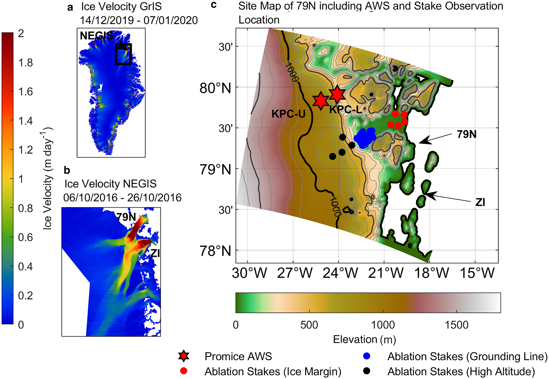
Ice velocity of the GrIS from 14 December 2019 to 7 January 2020 (a) and the NEGIS from 6 October to 26 October 2016 (b) (Solgaard and Kusk, Reference Solgaard and Kusk2019). Site map of the 79N and the lower drainage basin of the NEGIS (c). The map in (c) shows the elevation taken from the PWRF output and presents the modeled domain. The isolines indicate 100 m (gray) and 1000 m (black) altitude steps. Stars show locations of the AWSs from PROMICE (Fausto and van As, Reference Fausto and van As2019) and points show the location of surface ablation stakes (Zeising and others, Reference Zeising, Neckel, Steinhage, Scheinert and Humbert2020).
The floating tongue of the 79N Glacier directly connects the GrIS to the Atlantic Ocean (Schaffer and others, Reference Schaffer2017). It is ~8 km wide at the grounding line and extends ~80 km long into the Nioghalvfjerds fjord. At the terminus, the glacier tongue widens to ~30 km (Thomsen and others, Reference Thomsen1997; Reeh and others, Reference Reeh, Mayer, Miller, Thomsen and Weidick1999; Reeh and others, Reference Reeh, Mayer, Olesen, Christensen and Thomsen2000). The glacier thickness increases from ~50 m at the glacier margins to 250–600 m at the grounding line (Huybrechts and others, Reference Huybrechts, Mayer, Oerter and Jung-Rothenhäusler1999; Reeh and others, Reference Reeh, Mayer, Olesen, Christensen and Thomsen2000; Schaffer and others, Reference Schaffer2016). The inland extent of the glacier is difficult to outline, as it joins with Zachariae Isstrøm (ZI) and Storstrømmen Glaciers to become the NEGIS. However, the glacier outlines can be approximately determined by the high ice velocity compared to the surrounding ice sheet (Fig. 1b; Krieger and others, Reference Krieger, Floricioiu and Neckel2020).
The 79N Glacier was assumed to be stable until the early 21st century (Joughin and others, Reference Joughin, Smith, Howat, Scambos and Moon2010). However, recent observations revealed increasing surface velocities and glacier thinning (Khan and others, Reference Khan2014). Dynamical mass loss through numerous small calving events led to an area reduction of ~65.4 km2 between 1999 and 2013 (Jensen and others, Reference Jensen, Box and Hvidberg2016). This is ~4% of the total area of the floating portion of the glacier. Andersen and others (Reference Andersen2019) reported an average annual area change of ~−2.7 km2 a−1 from 1999 to 2018. Additional retreat is now likely following the 100 km2 calving of Spaltegletsjer (a tributary of 79N) in 2019 and 2020 (personal communication from Jason Box, 4 September 2020). The glacier is exposed to both changes in atmosphere and ocean circulation. The trapping of relatively warm Atlantic water under the glacier tongue by a sill leads to a basal melt rate of 10.4 ± 3.1 m a–1 (Schaffer and others, Reference Schaffer2020). Enhanced basal melting in particular years is likely driven by atmospheric processes which drive additional warm water into the cavity of beneath the floating tongue (Münchow and others, Reference Münchow, Schaffer and Kanzow2020). Additional variability in the mass balance (MB) comes from the surface mass balance (SMB) changes (Mouginot and others, Reference Mouginot2019). The 79N Glacier region has experienced 3°C warming of the average air-temperature over the last 40 years (Turton and others, Reference Turton, Mölg and van As2019a), and persistent supraglacial melt lakes now feature on both the floating tongue and grounded part of the glacier (Leeson and others, Reference Leeson2015; Hochreuther and others, Reference Hochreuther, Neckel, Reimann, Humbert and Braun2021). The equilibrium line altitude (ELA) is likely to increase in altitude within the 21st century (Leeson and others, Reference Leeson2015; Noёl and others, Reference Noёl, van de Berg, Lhermitte and van den Broeke2019).
Due to the remoteness of the 79N Glacier there are only a couple of SMB measurements and climate observations from automatic weather stations (AWSs) available (Fig. 1). Therefore, to estimate SMB of the glacier, models are valid tools. Several studies have been conducted recently concerning SMB of Greenland. Those attempts use diverse models such as the regional atmospheric climate model RACMO2 (e.g. Ettema and others, Reference Ettema2009; Noёl and others, Reference Noёl2018; Mouginot and others, Reference Mouginot2019), the Modèle Atmosphérique Régional (MAR) (e.g. Fettweis, Reference Fettweis2007), a degree-day model (e.g. Mayer and others, Reference Mayer2018) or other climate-SMB models (e.g. The IMBIE Team, 2020) to detect mass changes, and flowline models to simulate ice velocity and glacier outlines (Krieger and others, Reference Krieger, Floricioiu and Neckel2020). Others achieved their results concerning the MB or ice thickness change with data from satellite missions or from other air-borne surveys (e.g. Seroussi and others, Reference Seroussi2011; Khan and others, Reference Khan2014). However, common focus was set on mass changes of the entire GrIS on a rather coarse grid and NEGIS was treated as a part of GrIS. This leads to an underrepresentation of the large spatial and temporal variability of SMB in the 79N region which cannot be captured in a coarse grid in its full entity (Mayer and others, Reference Mayer2018; Noёl and others, Reference Noёl2018; Turton and others, Reference Turton, Mölg and van As2019a).
Prior to the current study, high-resolution SMB modeling down to a spatial resolution of 2.5 km was only available until 1997 (Huybrechts and others, Reference Huybrechts, Mayer, Oerter and Jung-Rothenhäusler1999). Therefore, recent intensive melt events or the effects of warm air advection during winter (Turton and others, Reference Turton, Mölg and van As2019a), are not incorporated or poorly resolved by coarser-resolution SMB models which simulate the whole of Greenland. Other unsolved questions include the ratio of meltwater that runs off into the ocean, refreezes or is stored as liquid water in ice pores or meltwater ponds. Previously, Turton and others (Reference Turton, Mölg and Collier2020) applied the Polar version of the Weather Research and Forecasting Model (PWRF) with 1 km spatial resolution on the domain shown in Figure 1c, to investigate the dominant atmospheric processes and climatology of the region. The current study attempts to link the PWRF atmospheric output with a recently developed SMB model called the COupled Snowpack and Ice surface energy and mass-balance model in PYthon (COSIPY) (Sauter and others, Reference Sauter and Arndt2020). COSIPY was previously tested for Himalayan glaciers (Sauter and others, Reference Sauter and Arndt2020) with observations from AWS as atmospheric input. However, as yet, COSIPY has not been tested in a one-way, offline coupled setting, using high-resolution 4-D model output from an atmospheric model as input. Here, we use the PWRF data as input and explore which parameter settings for COSIPY are appropriate for our region of interest. The goals of this study are twofold. First, we evaluate the accuracy of COSIPY in its ability to simulate the SMB when linked with PWRF. Second, once we have confidence in the model for this region, we use it to produce a high-resolution (1 × 1 km) dataset of SMB for the 79N Glacier. This study will provide a basis for studying the acceleration of mass loss in the 79N region further and to investigate the relationship between specific atmospheric processes and SMB. The modeled data (available from www.doi.org/10.5281/zenodo.4434259) can provide the foundations of a deeper understanding of the processes effecting the MB of this remote region.
The paper continues with a description of the COSIPY model and the observations used to manually optimize and evaluate the model (Section 2). The results are split into different sections, beginning with model optimization and evaluation (Section 3.1) and followed by presentation and discussion of the surface mass and energy balance for the 79N Glacier from 2014 to 2018 (Section 3.2). The paper concludes in Section 4.
2. Data and methods
The concept of driving a process-based MB model with high-resolution atmospheric model output over multiple years was successful for mountain glaciers (e.g. Mölg and others, Reference Mölg, Maussion and Scherer2014), and hence it seems a promising approach for the current study. Furthermore, due to the sparse atmospheric observations in the region and the large area of 79N, using high-resolution input from an atmospheric model, as opposed to localized in situ observations, should yield more accurate results with regard to spatial variability. Several in situ observations of SMB, radiation and near-surface meteorological data are used for model optimization and evaluation of the results. Table 1 lists all data used in this study.
List of input data from PWRF, AWS and stake observations including the time span of data usage and used variables

a 2 m air-temperature, 2 m air-pressure, incoming shortwave radiation, incoming longwave radiation, snowfall, total precipitation, wind-speed (horizontal wind vectors), initial information (skin temperature, water content, snow height, total height).
b Surface temperature, outgoing longwave radiation, shortwave albedo, snow height.
c Surface height change.
2.1. Study site
The regional climate is dominated by the characteristic annual cycle of the high-Arctic region, with the polar night (October to April), when no sunlight reaches the area, and the polar day (April to September). Two AWSs from the PROMICE network are located on the Kronprins Christian Land, just north of the 79N Glacier. A lower station is located in the ablation zone (KPC-L; where L stands for lower) and an upper station is near the equilibrium line (KPC-U; where U stands for upper; Fig. 1; Fausto and van As, Reference Fausto and van As2019). Cold conditions with annual mean temperatures (2009–18) of −13.4 ± 1.5°C (KPC-L) and −16.6 ± 0.5°C (KPC-U) characterize the local climate (Turton and others, Reference Turton, Mölg and van As2019a). The average summer temperature does not exceed the melting point at KPC-U, although daily maximum values can reach up to 4°C (Turton and others, Reference Turton, Mölg and van As2019a). Katabatic winds dominate the wind conditions. The strong temperature variability during winter is due to a combination of regional scale meteorological conditions, such as warm air advection from passing storms (Turton and others, Reference Turton, Mölg and van As2019a), and large-scale variability associated with teleconnections (Lim and others, Reference Lim2016; Hahn and others, Reference Hahn, Ummenhofer and Kwon2018).
2.2. Input data from Polar WRF
Data for the initialization of COSIPY comes from a high-resolution (1 km) Polar WRF (PWRF) output. PWRF is a polar-optimized version of the WRF model (Hines and others, Reference Hines and Bromwich2008). The atmospheric modeling was conducted and evaluated by Turton and others (Reference Turton, Mölg and Collier2020) using version v3.9.1.1 of PWRF. The output is available online (https://osf.io/53e6z/; last accessed on 9 May 2020). The data are available at hourly resolution for the domain shown in Figure 1c. Model outputs for this study from July 2014 to December 2018 are used. July 2014 is treated as a spin-up period, to ensure a minimum snow height (or no fresh snow as observed by a monthly average albedo of 0.47 at KPC-L, representing bare ice; Ryan and others, Reference Ryan2019) at the glacier surface starting August 2014 (Section 2.4). The experiment setup and parameterization for the PWRF modeling are described in Turton and others (Reference Turton, Mölg and Collier2020).
2.3. Observations
2.3.1. PROMICE weather stations
COSIPY is optimized with observations from two AWSs just north of 79N Glacier at two altitudes at the Kronprins Christian Land (Fig. 1c). KPC-L, in the ablation zone has an elevation of 255.6 m a.s.l., KPC-U is located near the equilibrium line at an elevation of 907.2 m a.s.l. (Table 1). The data are corrected (e.g. tilt-correction) and quality controlled according to the procedure by van As (Reference van As2011) and are available online at the PROMICE homepage (http://www.promice.org/PromiceDataPortal/; last accessed on 10 May 2020; Fausto and van As, Reference Fausto and van As2019). However, measurement errors cannot be completely excluded (Turton and others, Reference Turton, Mölg and van As2019a). Data from these locations were previously used to evaluate the PWRF atmospheric and radiation variables (Turton and others, Reference Turton, Mölg and Collier2020). To handle the noise in the snow height data, daily changes are calculated as difference in ‘midnight’ values defined as mean of all hourly values between 22:00 and 02:00 local time (LT), following Mölg and others (Reference Mölg2020). For COSIPY optimization the PROMICE data from January to December 2015 are used, as there are no missing values for all required input variables; the evaluation of COSIPY-WRF spans from August 2014 to December 2018 (Table 1).
2.3.2. Stake observations
In situ data from a field campaign conducted by the Alfred Wegener Institute (AWI) as a contribution to the Greenland Ice Sheet Ocean Interaction project (https://groce.de/en/; last accessed on 10 May 2020) are also used for independent evaluation of COSIPY-WRF. The observations are previously unpublished surface ablation estimates using ablation stakes on the 79N Glacier (Fig. 1c). Data are available for download from https://doi.pangaea.de/10.1594/PANGAEA.922131 (Zeising and others, Reference Zeising, Neckel, Steinhage, Scheinert and Humbert2020). The ablation stakes were installed in July 2017 and observations of snow height were taken in July 2018, which give the height change at the stake sites for 1 year. At each site, four stakes were installed, to prevent data loss in case of a failure of one stake, and to provide uncertainties in surface height change estimates.
The elevation and location of the stakes was recorded with a GPS device which has an elevation accuracy of ~10 m. The elevation of the stakes on the floating tongue is also subjected to an additional error of 3 m due to the tidal movement. We used the coordinates of the GPS to select the closest gridpoint in the COSIPY-WRF output for comparison. The uncertainties in stake location do not translate to an uncertainty of the surface height change, but to the elevation of the stake observations (personal communication from Zeising, 5 February 2020). The measured GPS locations are listed in Table 4 in Appendix A.
2.4. COSIPY
2.4.1. Structure and optimization
COSIPY is available online in its current release as an open-source software, we use v1.1 for this study (https://github.com/cryotools/cosipy; last accessed on 9 May 2020; Sauter and Arndt, Reference Sauter and Arndt2020). It is a physical surface energy and MB model that assumes full mass conservation in the snowpack. Therefore, it calculates the different mass fluxes by distinguishing between internal mass balance (IMB) and SMB. The sum of IMB and SMB is the total MB (TMB). In COSIPY, IMB summarizes the subsurface melt and the refreezing of meltwater, and SMB summarizes all MB processes at the surface including surface melt, snowfall, sublimation and deposition. Excess meltwater can be held in the snow layers as liquid water content. If one layer is saturated, meltwater drains in the next layer below (tipping bucket approach) or runs off when it reaches the surface below the lowest model layer (Sauter and others, Reference Sauter and Arndt2020). By doing so, the model divides the snow and ice pack into several user-defined numbers of layers in the vertical (Sauter and others, Reference Sauter and Arndt2020).
The ablation component relies on the surface energy balance (SEB). An energy surplus at the surface can cause melting (if the surface temperatures reach 0°C). A negative SEB, on the other hand, causes cooling of the surface layers. Sublimation or deposition also occurs depending on the surface-air water vapor pressure gradient between the surface and the surface layer. In COSIPY, SMB is computed as the difference of the total accumulation at the surface (snowfall accumulation and deposition) and the total ablation at the surface (surface melt and sublimation). Penetrating energy into the snowpack triggers ablation processes in the snowpack. Here, ablation occurs due to internal melting if temperatures reach 0°C. Melt water from surface and subsurface melt can penetrate deeper snow layers and refreeze there too or is held in pores as liquid water content. Excess meltwater contributes to the runoff and leaves the domain (Sauter and others, Reference Sauter and Arndt2020).
Carefully chosen parameter settings are needed to produce an ‘optimal’ model performance of COSIPY in this Arctic setup. For this reason, and as COSIPY is a newly released SMB model, a manual trial-and-error approach is preferred over an automated Monte-Carlo approach which is used for long-term documented MB models (e.g. Mölg and others, Reference Mölg, Maussion, Yang and Scherer2012; Cullen and others, Reference Cullen, Mölg, Conway and Steffen2014). A manual testing of parameter tuning gives a better idea of the response of COSIPY results to changes in the configuration. The testing followed the value ranges in Tables 5 and 6 in Appendix B and the final parameter selection is presented in Table 2. Input data from the two PROMICE AWSs are used from January to December 2015 for optimization (Section 2.3.1). In a second step, the model is applied to the 79N domain using the PWRF data as input.
Parameterization and parameters selection for the COSIPY-WRF run

References are provided where value/value ranges have been used from previous studies. Each parameter was tested according to the options and ranges indicated by Tables 5 and 6 in Appendix B.
The initial englacial vertical profiles of the state variables temperature, liquid water content and density needed for the optimization are from the observations. The top-layer and bottom-layer temperatures are the mean temperatures of December 2014 and January 2015 measured at the surface and 10 m depth by the PROMICE AWSs (248.40 ± 6.4 K top, and 260.46 ± 0.6 K bottom for KPC-L; 244.87 ± 7.0 K top, and 258.66 ± 0.1 K bottom for KPC-U) (Table 2). Even though the 79N Glacier is reported to be much thicker than 10 m (e.g. Schaffer and others, Reference Schaffer2016), the assumption regarding the constant bottom-layer temperature is reasonable. The conductive heat flux below that depth was regarded to be negligible over the timescale examined following Cullen and others (Reference Cullen, Mölg, Conway and Steffen2014).
In COSIPY, the albedo is calculated with the parameterization of Oerlemans and Knap (Reference Oerlemans and Knap1998). The strong variability of ice albedo, which can range from 0.1 to 0.6 depending on the surface conditions, makes it difficult to find values for the entire 79N Glacier (Bøggild and others, Reference Bøggild, Brandt, Brown and Watten2010). Manual testing and inspection of the AWS data revealed that the albedo decreases from a fresh snow albedo of 0.87 to a firn albedo of 0.78 with an aging factor of 2 d after the snowfall event. When there is no snow layer, the albedo drops to 0.525 (van de Wal and Oerlemans, Reference van de Wal and Oerlemans1994). The depth scaling factor for albedo was found to be 12.5 cm (Table 2). The non-reflected shortwave radiation heats the surface, penetrates the snowpack and supplies the interior with energy according to Bintanja and van den Broeke (Reference Bintanja and van den Broeke1995). The outgoing longwave radiation is calculated after updating the surface temperature assuming a final surface emissivity of 0.99, following Noёl and others (Reference Noёl2018) (Table 2).
To calculate the turbulent heat fluxes, COSIPY assumes a linear roughness length increase with time following Mölg and others (Reference Mölg, Cullen, Hardy, Winkler and Kaser2009). The maximum increase from a fresh snow value of 0.5 mm to a firn value of 1.7 mm (Smeets and van den Broeke, Reference Smeets and van den Broeke2008; Fausto and others, Reference Fausto2016) occurs if there is no new snow addition over a specified time window, which has the same length as the albedo aging factor (Mölg and others, Reference Mölg, Cullen, Hardy, Winkler and Kaser2009). A value of 3.5 mm is assumed for bare ice (Cullen and others, Reference Cullen, Mölg, Conway and Steffen2014). The stability influence on the sensible and latent heat fluxes is based on the Richardson number (Table 2; Braithwaite, Reference Braithwaite1995).
Surplus energy results in ablation. If the surface temperature is below 273.16 K, only sublimation can occur. If the surface temperature exceeds the freezing point, it is set to a melting temperature of 273.16 K and the excess energy is translated into melt energy (Sauter and others, Reference Sauter and Arndt2020). Aging snow layers decrease their height due to compaction and densification. The density calculation with the ‘Boone’ method is described in Essery and others (Reference Essery, Morin, Lejeune and Ménard2013). Thereby, the density threshold of ice is 800 kg m−3 (Herron and Langway, Reference Herron and Langway1980). The threshold of firn is derived after manually testing parameter combinations following the tested range in Cullen and others (Reference Cullen, Mölg, Conway and Steffen2014) from 400 to 500 kg m−3. A minimum firn density of 400 kg m−3 was selected as it produces results closest to the observations (Table 2).
2.4.2. COSIPY-WRF configuration
The final COSIPY-WRF run was initiated on 15 July 2014. For the COSIPY-WRF simulations, the constant bottom-layer temperature was 258.7 K (the mean value for the observations at both AWSs) and was run with only the final set of parameters after the manual optimization. The first 15 d are regarded as a spin-up and are not included in the analysis. The spin-up includes the last 2 weeks of July where no snow accumulation was modeled or observed. The analyzed COSIPY-WRF output starts from 1 August 2014 (Table 1). At this time there is no fresh snow and minimal old snow observed and modeled at the glacier surface facilitating the initialization process of the model. The comparison against SEB terms and SMB from PROMICE AWSs is conducted for hourly values, except for albedo, for which a daily mean value is calculated. Albedo values are calculated as the sum of the observed outgoing shortwave radiation divided by the sum of the observed incoming shortwave radiation in 1 d. This approach is suggested by Oerlemans and Knap (Reference Oerlemans and Knap1998) to reduce errors from hours of low solar elevation.
3. Results and discussion
3.1. Model evaluation
3.1.1 Optimization period (January to December 2015)
In order to optimize the model set up, all time steps of year 2015 (1 January to 31 December) are evaluated according to the correlation coefficient (R) and the root mean square error (RMSE) to the PROMICE AWSs (Table 3). COSIPY-WRF simulates the observed conditions at both AWSs well in the optimization period. The model results agree with the measurements with relatively high significant correlation coefficients and a low RMSE (Table 3). For surface temperature, COSIPY-WRF archives a performance comparable to Huintjes and others (Reference Huintjes2015) (R = 0.95, RMSE = 3.44 K for KPC-L, and R = 0.94, RMSE = 2.03 K for KPC-U, compared with R = 0.98, RMSE = 2.12 K in Huintjes and others, Reference Huintjes2015). The evaluation statistics for albedo (R = 0.78, RMSE = 0.10 for KPC-L, and R = 0.62, RMSE = 0.12 for KPC-U) compare well with the statistics archived by Mölg and others (Reference Mölg, Cullen, Hardy, Kaser and Klok2008) (R = 0.69, RMSE = 0.10). This suggests a reasonable level of optimization.
Evaluation statistics (correlation coefficient – R and root mean square error – RMSE) for COSIPY-WRF evaluation against PROMICE AWSs in the optimization and the evaluation period

The statistics for the evaluation period were calculated one time for the entire time series and a second time for the time series excluding the optimization period.
3.1.2 Model evaluation from August 2014 to December 2018
A longer-term model evaluation of COSIPY-WRF is conducted for the period from 1 August 2014 to 31 December 2018. The statistical comparisons are also included in Table 3; a visual comparison is presented in Figures 2 and 3 for KPC-L and KPC-U, respectively. The comparison against the observation from PROMICE AWSs reveals a good agreement of COSIPY-WRF with the observed surface temperature (R = 0.92, RMSE = 4.46 K for KPC-L, and R = 0.90, RMSE = 5.13 K for KPC-U) and outgoing longwave radiation (R = 0.92, RMSE = 16.73 W m−2 for KPC-L, and R = 0.91, RMSE = 18.78 W m−2 for KPC-U) (Figs 2a, b, 3a, b). For both variables, the simulated time series follow the annual cycle of the measurements and meet the values relatively accurately. The statistical evaluation for the surface temperature is similar to the evaluation in Sauter and others (Reference Sauter and Arndt2020). Statistics for the outgoing longwave radiation are similar to those considered as good in Noёl and others (Reference Noёl2018; R = 0.98 and RMSE = 14.20 W m−2 at their station S5). When excluding the optimization period from the evaluation period there is no systematic decrease in the model performance (Table 3).
Model evaluation against the KPC-L of hourly surface temperature (a), hourly outgoing longwave radiation (b), daily shortwave albedo (c) and accumulated hourly surface height change relative to the first time step (d). The time period is 1 August 2014 00:00 to 31 December 2018 23:00 LT. The blue-dashed lines indicate the start and end time of the optimization period. Due to a measurement error of the SR50 sensor for the snow height change (stripping), the time before 1 July 2015 was excluded from evaluation for the snow height evaluation. Snow height can drop below zero due to a small initial snow layer at the observation site.

Model evaluation against PROMICE the KPC-L AWS of hourly surface temperature (a), hourly outgoing longwave radiation (b), daily shortwave albedo (c) and accumulated hourly surface height change relative to the first time step (d). The time period is 1 August 2014 00:00 to 31 December 2018 23:00 LT. The blue-dashed lines indicate the start and end time of the optimization period. Snow height can drop below zero due to a small initial snow layer at the observation site.

The albedo is modeled with a relatively high correlation coefficient of R = 0.85 for KPC-L and R = 0.67 for KPC-U (Figs 2c, 3c; Table 3). At KPC-L, the decrease in albedo during summer, when ice is exposed, is delayed in the simulations (Fig. 2c). This is a result of finding the best albedo parameters valid for the entire 79N Glacier. To meet the KPC-L albedo values, a lower ice albedo and a higher scaling factor would produce a better model fit. However, a higher ice albedo and a lower albedo aging scaling factor produce a better agreement with the KPC-U albedo values. A similar difficulty in albedo parameterization choice for a large heterogeneous ice surface was identified by Noël and others (Reference Noёl2018). In previous studies, a better agreement in albedo values between observations and simulations were achieved by advancing the albedo parameterization of Oerlemans and Knap (Reference Oerlemans and Knap1998). For instance, Helsen and others (Reference Helsen2017) included both wet and dry snow albedos and various albedo aging factors. However, COSIPY does not currently have the option to choose wet vs dry albedos; therefore, we selected the most appropriate albedo values based on manual optimization of the model (Section 2.4.1 and Table 2).
In terms of snow height change, an offset is evident at both stations (Figs 2d, 3d). Especially at KPC-L, the modeled snow height is too high in winter 2015. This is partly attributed to errors in the measurements during the accumulation period. The albedo and snow height at KPC-U remain high, indicating snow cover, whereas at KPC-L, snow height is much lower despite the high albedo value. Note that the values in Figures 2d, 3d can be negative as it is a relative change since the first date of the simulation (1 August 2014) when a small layer of snow was present on the surface. The sonic rangers used to measure the distance between the surface and the sensor have a membrane which deteriorates over time and produces erroneous values (personal communication from van As D, 22 August 2019), which is a known potential problem with these instruments (Mölg and others, Reference Mölg2020). Therefore, a number of time steps from August 2014 until July 2015 were left out while calculating the evaluation statistics resulting in an RMSE of 0.39 m (Fig. 2d). COSIPY-WRF still overestimates the snow height observations at KPC-U but results in a smaller RMSE of 0.32 m compared to the RMSE at KPC-L (Fig. 3d). After summer 2015, the agreement of modeled and observed snow height improves for both PROMICE AWSs. A positive model bias in snow height can also result from a number of things, including an underestimation of the density by the parameterization. Due to the large area of 79N Glacier, finding a valid density parameter is difficult, as no density observations are available for this location. We tested both the ‘Bonne’ and ‘Vionnet’ parameterizations available in COSIPY and found higher agreement with observations for the Boone method. For the final run, the ‘Boone’ method was used as this was also reported to produce the best fit in previous studies (e.g. Essery and others, Reference Essery, Morin, Lejeune and Ménard2013). We chose this parameterization, despite having no observations to assess its validity for the 79N Glacier region. Issues in snow height simulation also rise from the effects of snowdrift that are not simulated by PWRF. Previous studies have shown a significant effect of snowdrift on the snow height in eastern Greenland (Hasholt and others, Reference Hasholt, Liston and Knudsen2003).
Figure 4 compares the modeled height change with the observations from the ablation stakes. Negative values point to ablation and decreasing surface height and positive values indicate accumulation and increasing surface height between July 2017 and July 2018. COSIPY-WRF overestimates ablation at some of the stake locations. At the glacier margin (five stakes; red points in Fig. 4), the modeled ablation is stronger compared to the measurements resulting in an RMSE of 0.97 m. At the stakes near the grounding line (blue points in Fig. 4), this offset decreases. Here, the COSIPY-WRF results agree better with the observations (RMSE = 0.32 m). Some ablation stakes at higher altitudes point to either ablation or accumulation (five stakes: black points in Fig. 4). COSIPY-WRF simulates ablation well at the stakes affected by a decreasing surface. However, the model results in a positive MB at only one of the three sites with observed accumulation. This points to a modeled 2017–18 ELA that is too high. Altogether, this leads to an RMSE of 0.67 m in the high-altitude group. The errors can be attributed to various reasons, such as measurement error related to tidal movement of the floating parts of the glacier tongue and GPS errors in elevation (see Section 2.3.2) (Reeh and others, Reference Reeh, Mayer, Olesen, Christensen and Thomsen2000; Joughin and others, Reference Joughin, Smith, Howat, Scambos and Moon2010; personal communication Zeising, 5 February 2020). The inaccuracy of the GPS sensors at the ablation stakes makes it difficult to find the exact gridpoint for the comparison with COSIPY-WRF (personal communication Zeising, 5 February 2020).
Comparison of the modeled glacier height change with the GPS measurements at the ablation stakes from AWI. At each site, four stakes were deployed to prevent data loss in case of the failure of one stake and to provide error estimates. The error bars indicate the SD of the measured values at each site. Coloring shows reference to the location of the measurement sites like in Figure 1 (red: ice margin, blue: grounding line, black: high altitude region).

In spite of these significant measurement uncertainties, the simulated height change agrees relatively well with the observations. The model fit is highest at locations near the grounding line. The RMSE increases toward the lower areas of the floating tongue and toward the ELA. The floating tongue is highly crevassed and features many small melt ponds and channelized melt areas (Hochreuther and others, Reference Hochreuther, Neckel, Reimann, Humbert and Braun2021) making it difficult to find appropriate places for stake observations. The ELA in the 2017–18 ablation period was lower than that in previous years, as the accumulation during winter 2017 to 2018 was more intense than previous years (Turton and others, Reference Turton, Mölg and Collier2020; Section 3.3), which could be partially responsible for a poorer agreement between observations and simulations at the lower elevations. All in all, the evaluation against PROMICE AWSs and ablation stake measurements shows that COSIPY-WRF in its current configuration can offer a realistic estimate of SMB and SEB of the 79N Glacier and is therefore analyzed further in Section 3.2.
3.2. SMB and IMB
The modeled SMB is illustrated in Figure 5. The 79N Glacier features distinct patterns regarding the spatial distribution of annual SMB. The floating tongue is prone to negative SMB in all simulated years. There are variations in the estimates regarding the ELA and the extent of ablation in higher regions. Between September 2014 and August 2017, negative SMB regions exceed 1000 m a.s.l. In the 2014–15 period, SMB is negative up to an altitude of 1300 m a.s.l., however annual SMB total is small in magnitude accumulating to ~−13.56 × 10⁶ kg a−1 (Fig. 5a). The mass loss intensifies in the 2015–16 and 2016–17 periods, with annual SMB values of −25.51 × 10⁶ and −29.68 × 10⁶ kg a−1, respectively (Figs 5b, c). Lower annual ablation in 2017–18 at the glacier tongue is depicted in Figure 5d. In the 2017–18 period, annual accumulation at the surface is evident already at 500 m a.s.l. In this year, SMB accumulates to ~+5.75 × 10⁶ kg a−1.
Spatial distribution of the annual SMB from September to August of the following year starting 2014 (a), 2015 (b), 2016 (c) and 2017 (d). The contours indicate 100 m (gray) and 1000 m (black) altitude steps taken from WRF.

Often, a negative TMB results in enhanced meltwater production. The surface water collects into meltwater ponds or supraglacial lakes, as seen on the surface of 79N (Leeson and others, Reference Leeson2015; Ignéczi and others, Reference Ignéczi2016; Hochreuther and others, Reference Hochreuther, Neckel, Reimann, Humbert and Braun2021). From there, a portion of meltwater evaporates, refreezes or runs off. Meltwater that penetrates the snowpack can either refreeze englacially, be collected in subglacial lakes or runs off at the base. The latter can lubricate the bedrock and can accelerate the ice flow inducing instability to other parts of the glacier (Carr and others, Reference Carr, Stokes and Vieli2013; Rathmann and others, Reference Rathmann2017; Bevis and others, Reference Bevis2019). Figure 6 illustrate the portion of surface meltwater that refreezes, runs off, evaporates or is stored in the snowpack (Figs 6a, b, c, d). Furthermore, the contribution of SMB and IMB to TMB is illustrated. Figures 6e, f, g h depict the simulated cumulative annual IMB – refreeze minus subsurface melt – and SMB – snowfall and deposition minus surface melt, sublimation and evaporation – contributing to the TMB of the 79N Glacier. Surface melt is a dominant factor determining ablation at the surface (Section 3.3).
The ratio of surface meltwater that contributes to runoff, refreeze, evaporation or remains in the snow layer as liquid water content from September to August of the following year starting 2014 (a), 2015 (b), 2016 (c) and 2017 (d). The bottom panels show the contribution of SMB and IMB to the TMB of the same periods starting 2014 (e), 2015 (f), 2016 (g) and 2017 (h).

The major portion of the surface melt contributes to the runoff in all years, whereas evaporation is suppressed because of the low temperatures in the region (Fig. 9b in Appendix C). As a result, only 1% of the surface meltwater evaporates. Furthermore, a considerable part of meltwater is stored inside the snow layers. Schröder and others (Reference Schröder, Neckel, Zindler and Humbert2020) found evidence for liquid water retention under ice lenses and snow throughout the winter in our study area, which confirms that not all meltwater refreezes. Refreezing is more dominant in 2014–15 and 2017–18. This may be related to cooler climate conditions and low surface temperatures, which promote fast refreezing of meltwater before it runs off (Figs 9a, b in Appendix C).
Although during the 2014–15 and the 2017–18 periods (Figs 6e, h), IMB is the dominant factor for the TMB, the SMB does dominate over IMB in the periods from 2015–16 to 2016–17 (Figs 6f, g). The modeled TMB remains negative throughout the simulated time. In the years in which IMB is more negative than SMB, less than two-thirds of the meltwater contribute to the surface runoff (Figs 6a, d). In contrast, >85% of the total meltwater runs off in years when SMB contributes more to the TMB (Figs 6b, c). The only year with a positive component of the MB is 2017–18, but estimated positive SMB is compensated by negative IMB, resulting in an overall negative TMB.
SMB has a higher annual variability compared to IMB as it is more dependent on regional atmospheric conditions and its variability. Changes in meltwater runoff induce variabilities to the stability, the velocity and the total mass loss of the glacier (Fettweis, Reference Fettweis2007; Mayer and others, Reference Mayer2018; Bevis and others, Reference Bevis2019). The IMBIE Team (2020) supported that the meltwater production and runoff for the GrIS increased because of regional warming. Therefore, glacier-wide surface ablation can explain strong run off between 2015 and 2017. Furthermore, an overall negative MB in all periods agrees with Mouginot and others (Reference Mouginot2019). They identified an overall negative MB for the GrIS, which was largely due to internal and dynamic processes that did not allow accumulation due to surface processes even in years with positive SMB. This agrees with our findings for the 2017–18 period, when modeled positive SMB turns into a negative MB due to the IMB. Dynamical processes, such as iceberg calving or surging, are not included in the COSIPY model. However, during our study period, no major calving events were detected and 79N is not a surge-type glacier, unlike its southerly neighbor, Storstrømmen (Mouginot and others, Reference Mouginot2019).
3.3. Interannual variability of the SMB
The difference in SMB between the 2016–17 (Fig. 5c) and 2017–18 (Fig. 5d) years (which are the highest and lowest surface melt years in our study, respectively), prompted us to investigate the differences between the two years (hereafter ‘2017’ and ‘2018’). TMB and SMB exhibit distinct features. Ablation is strongly reduced in 2018 concerning both the total and the surface ablation (Figs 7b, d), whereas accumulation does not show large differences (Fig. 7a, c). Snowfall and surface melt during the ablation period are prominent components of SMB (Figs 7e, f, j), whereas deposition and sublimation are less dominant (Figs 7g, h, k, l). Due to the overall low surface and 2 m air-temperature, surface melting is suppressed and ablation due to sublimation gains importance in the accumulation period and in high altitude bands (Figs 7i, k; Figs 9a, b in Appendix C).
Average vertical profile (altitude bands of 50 m) of the TMB (a and b) and SMB (c and d), and the components of the modeled SMB. This includes snowfall from PWRF (e and f), deposition (g and h), surface melt (i and j) and sublimation (k and l). The red line shows results for 2016–17 and the blue line shows results for 2017–18. The data are averaged over the accumulation periods (October 2016 to April 2017, and October 2017 to April 2018) in light blue boxes and over the ablation periods (May to September 2017 and May to September 2018) in brown boxes.

Distinct and significant differences are evident regarding the strength of surface melt and snowfall (paired t-test). Although in 2017 intensive melting appears in the ablation period, the melting is reduced in 2018 (Fig. 7j). Simultaneously, snowfall increased at elevations below 1200 m in the ablation period of 2018 compared to 2017 (Fig. 7f). However, there was no significant difference in snowfall amount during the accumulation periods of the two years (Fig. 7e). Only in lower altitudes of the ablation zone does the surface melt exceed mass gain by snowfall, while snowfall accumulation is persistent, leading to a distinct and significant reduction in negative SMB values in 2018 compared to 2017 (paired t-test).
SMB features are also expressed by the SEB (Fig. 8). Energy surplus during the ablation period is caused by rising incoming shortwave radiation and decreasing albedo resulting in a high positive net shortwave radiation (Figs 8b, d, and Fig. 10b in Appendix C), whereas in the accumulation period the shortwave radiation budget is near zero and albedo values are high (Figs 8a, c, and Fig. 10a in Appendix C; Fausto and others, Reference Fausto2016; Hahn and others, Reference Hahn, Storelvmo, Hofer, Parfitt and Ummenhofer2020). In the 2017 accumulation period, the longwave radiation is more negative at lower altitudes than in 2018. In the 2017 ablation period, a more negative longwave radiation is simulated at higher elevations. Overall, this leads to a weaker longwave radiation deficit in 2017 compared to 2018 (Figs 8e, f, and Fig. 10d in the Appendix C; Turton and others, Reference Turton, Mölg and van As2019a). Sensible heat adds energy to the surface throughout the year (Figs 8g, h). Surface temperatures at the melting point initiate the conversion of excess energy to melt energy during the ablation period (Figs 8l, Fig. 9a in Appendix C). The low longwave radiation flux coupled with a negative latent heat flux and a lack of energy input by shortwave radiation and by sensible heat suppresses melt energy, which approaches zero in all altitude bands in the accumulation period 2018 (Fig. 8k).
Average vertical profile (altitude bands of 50 m) for the components of the SEB. This includes net shortwave radiation, SWnet (a and b), albedo (c and d), net longwave radiation, LWnet (e and f), sensible heat flux (g and h), latent heat flux (i and j) and melt energy (k and l) from COSIPY-WRF. The red line shows results for 2016–17 and the blue line shows results for 2017–18. The data are averaged over the accumulation periods (October 2016 to April 2017, and October 2017 to April 2018) in light blue boxes and over the ablation periods (May to September 2017 and May to September 2018) in brown boxes.

In the ablation period of 2017, the snow layer melted entirely, including at higher altitudes, resulting in the exposure of large extents of ice surface. As a consequence, the albedo was reduced and more shortwave radiation was absorbed and therefore available for ablation processes in summer 2017; a causality chain known to induce strong variability in MB also in other climatic zones (Mölg and others, Reference Mölg, Cullen, Hardy, Winkler and Kaser2009). This albedo feedback also explains positive SMB in the 2017–18 period. Higher snowfall in lower altitudes increased the snow height, which caused higher albedo and a decreased shortwave radiation budget at the surface. A lower snowline resulted in higher albedo, which reduced the melt energy and dampened surface melting in summer 2018. This snowline-albedo feedback at the margins of the GrIS was described for the period 2001–2017 by Ryan and others (Reference Ryan2019).
The COSIPY-WRF simulation points to a significantly warmer ablation period, especially in July, in terms of surface and air temperature in 2017 compared to 2018 in all altitude bands (paired t-test; Figs 9a, b in Appendix C). Additionally, wind speed and relative humidity from PWRF are significantly increased during both seasons in 2017 (paired t-test; Figs 9c, d in Appendix C). The differences in wind speed at the altitude bands near the grounding line are the only non-significant points (Fig. 9c in Appendix C). The strong and persistent wind speed in July 2017 promotes the intensification of turbulent energy fluxes in the ablation period (Figs 8h, j). Those increases in importance to SMB as other ablation processes (e.g. surface melt; Fig. 8i) are suppressed due to low temperatures. The respective mass turnover by sublimation and deposition has less of an impact on the TMB, however (Figs 7g, h, k, l). The snowfall (Fig. 7b) has a much larger impact on SMB, as seen over large parts of the glaciers in 2018 compared to 2017 (Figs 5c, d). In conclusion, less mass loss at the surface may be attributed to a significant increase in snowfall, and therefore albedo values, which was largely caused by a cooler regional climate in summer 2018 (The IMBIE Team, 2020).
4. Conclusion
The forcing of an SMB model with a high-resolution regional atmospheric model, PWRF, reproduced available observations reasonably well and enables more insights into mass changes in the remote area of the 79N Glacier. The manual model optimization conducted to meet the climatic observations from two PROMICE AWSs, however, also revealed problems in the parameterization for a large area. Often, input to SMB models, especially on smaller glaciers, comes from one or a few in situ observation sites (Mölg and others, Reference Mölg, Cullen, Hardy, Kaser and Klok2008; Sauter and others, Reference Sauter and Arndt2020). In this case, we attempted to find the best parameter selection for two stations, one in the ablation zone and one near the ELA, with quite different climatic characteristics. In addition, the simulation of snowfall and the related accumulation was a critical factor (Section 3.1). However, the modeled data from COSIPY-WRF were found to be suitable for a first detailed analysis of MB processes as response to atmospheric features.
SMB observations in this remote region are sparse and often plagued with difficulties. Independent stake data were only available for 1 year and were affected by tidal variations and GPS inaccuracies. However, our estimates of ~2 m mass loss on the floating tongue were also found in similar magnitude for NEGIS and 79N by Khan and others (Reference Khan2014). At the grounding line, the model results are more comparable with observations. Partially, this could be due to reduced tidal influence, but may also be due to parameter selections based on the KPC-L station, which is close to this location (Fig. 1).
The present results indicate stronger variability of ablation processes compared to accumulation processes on interannual timescale in the study domain. SMB features are dominated by ablation over the 79N Glacier in 2014–17 and turn positive in 2018. A major reason for this change in sign of the SMB is a strong variability in surface melt rates. In intense ablation years (September 2015 to August 2017) the mass loss due to surface ablation dominates the impact of IMB, and a major part of the meltwater contributes to the surface runoff. This finding is reversed in years with less overall ablation (September 2014 to August 2015) or positive SMB (September 2017 to August 2018). In those years, dominant factors inducing mass loss are components of IMB while SMB is small or positive. Also, most of the meltwater does not contribute to the surface runoff in those years. The TMB in the analyzed period remains negative (Fig. 6).
The COSIPY-WRF results reveal a substantial interannual variability in surface ablation, such as the reduced values in 2018, which can be explained by the effects of a cooler regional climate. The main differences between 2018 and the previous years with more intense overall ablation are increased snowfall, decreased surface melt and consequently higher albedo and lower net shortwave radiation budget in summer 2018. This difference effects large parts of the higher regions of the 79N Glacier, while being insignificant on the glacier tongue. Therefore, the climate in the lower ablation zone is potentially less influential over interannual SMB variability.
The low overall temperatures in this region suppress the ablation processes such as surface melting. Especially in the accumulation period, when the mean temperatures do not exceed the melting point, sublimation and deposition rise in importance, but remain in a low quantity. Melting at the NEGIS and 79N including the floating tongue occurs almost exclusively in June to August when net shortwave radiation is positive. In conclusion, the presented dataset reproduces SMB and SEB at the 79N Glacier reasonably well and highlights the large spatial and interannual variability of SMB and the individual components. The high resolution of SMB output is beneficial for future investigation into interactions between specific atmospheric features or extreme events, and the mass and energy balance of the 79N Glacier.
Acknowledgements
We thank Ole Zeising from the Alfred-Wegener Institute (AWI) for providing the data from the ablation stakes at the 79N Glacier and for additional information and communication throughout the project. Thanks are also to Prof. Jason Box for his information on the calving of 79N. This study was supported by the German Federal Ministry for Education and Research (BMBF) with grant number 03F0778F. We acknowledge the High-Performance Computing Centre (HPC) at the University of Erlangen-Nürnberg's Regional Computation Centre (RRZE), for their support and resources while running the COSIPY simulations. Daily average values of the SMB components from July 2014 to December 2018 are available online and open access at: www.doi.org/10.5281/zenodo.4434259. We express our thanks to the two anonymous reviewers and the editor for providing reviews of the paper, which benefitted from their critiques.
Author contributions
M.T.B. conducted optimization, simulation and evaluation of the COSIPY-WRF model and wrote the manuscript. J.V.T. designed the study. T.S. provided assistance in the setup and running of the model. T.M. assisted with model optimization and evaluation. J.V.T, T.S. and T.M. contributed to writing the manuscript and discussion of the results.
Conflict of interest
The authors confirm that they have no conflict of interest.
Appendix A: Ablation stake locations
See Table 4.
GPS locations of the ablations stakes and the measurement results

Appendix B: Manual optimization scheme
List of parameterization options available in v1.3 COSIPY (Sauter and others, Reference Sauter, Arndt and Schneider2020)

List of key parameters and the range of values tested in model optimization

Appendix C: Local climate and radiative conditions
Average vertical profiles (altitude bands of 50 m) for the surface temperature from COSIPY-WRF (a) and the mean climate conditions – 2 m air-temperature (b), 2 m wind speed (c) and relative humidity – from the PWRF output at the 79N region in July 2017 and July 2018. The surface temperature.

Average vertical profile (altitude bands of 50 m) for the components of incoming shortwave radiation, SWin (a and b) and incoming longwave radiation, LWin (c and f) from COSIPY-WRF with energy flux density on the x-axis. The data are averaged over the accumulation periods (October 2016 to April 2017, and October 2017 to April 2018) and over the ablation periods (May to September 2017 and May to September 2018).


 Open access