INTRODUCTION
As long as people have worked with calibrated radiocarbon (14C) dates, there has been a wish to summarize large numbers of calibrated dates in an effective way. The issues involved can be separated into two classes: dealing with systematic biases in the datasets due to survival or sampling probability, and artifacts which are generated by many of the most widely used methods for presentation of data. This paper seeks to address the second of these two problems while acknowledging that the taphonomic biases are in many cases the most important issue. The overall aim is to find a better way to determine the temporal density of ages, as reflected in large 14C datasets, where there is no clear prior information on their distribution.
The fact that dates with errors always appear to be more spread than they really are was carefully considered by Buck et al. (Reference Buck, Litton and Smith1992) where they introduced the approach of making use of prior information that events are grouped within phases, under the assumption that they are uniformly likely to be anywhere within each phase. This approach can be widened to include other types of distribution such as normal, triangular (Bronk Ramsey Reference Bronk Ramsey2009) and trapezoidal (Karlsberg Reference Karlsberg2006; Lee and Bronk Ramsey Reference Lee and Bronk Ramsey2012; Bronk Ramsey and Lee Reference Bronk Ramsey and Lee2013). All of these approaches reduce the chronology to a set of model parameters such as the start and end and duration of a uniform phase. In many cases, it is sufficient to plot and quote the ranges for these parameters to explain the significance of the data (Bayliss et al. Reference Bayliss, Bronk Ramsey, van der Plicht and Whittle2007). This type of analysis constitutes much of the Bayesian chronological analysis currently being undertaken in Archaeology.
Two issues are not fully dealt with in this way however. The first arises in situations where, for example, a uniform phase model is applied and yet there is still a requirement to look at the distribution of events within that phase or to summarize that distribution in some way. The second is where there is no prior information available to postulate a phase with a particular underlying distribution. This latter case is particularly common when looking at large datasets over long time periods in order to assess the implications of climatic and other environmental influences (see for example Stuart et al. Reference Stuart, Kosintsev, Higham and Lister2004; Ukkonen et al. Reference Ukkonen, Aaris-Sørensen, Arppe, Clark, Daugnora, Lister, Lõugas, Seppa, Sommer and Stuart2011; Buchanan et al. Reference Buchanan, Collard and Edinborough2008; Shennan Reference Shennan2013).
Many different approaches have been used to summarize datasets, including binning of ranges, summing calibrated date distributions, binning the output of such sums and simulation methods. There are three main problems that arise in these methods: excessive noise seen in summed distributions, over-smoothing of the data if techniques are used to remove this noise, and a failure to address the issue of statistical spread unless they are combined with other forms of Bayesian analysis. Some of the methods are also complex to implement and therefore not suitable for widespread use in visualizing datasets. The main purpose of this paper is to explore methods based on Gaussian (normal) Kernel Density estimation in order to asses whether they might be a useful tool in summarizing 14C datasets with and without other forms Bayesian analysis.
CURRENT METHODS OF SUMMARIZING 14C DATASETS
There are a number of different ways people have used to present multiple 14C dates. The first is simply to plot multiple distributions, which can be done with any of the widely used calibration software packages. The challenge is how to summarize many such plots, or to understand their significance.
The older literature contains a very wide variety of methods, including the binning of uncalibrated dates or mean dates. Clearly these are not ideal except for the roughest of analyses. More sophisticated methods using the ranges from calibrated datasets have also been used (see for example MacDonald et al. Reference MacDonald, Beilman, Kremenetski, Sheng, Smith and Velichko2006) often together with some form of running mean. These methods are often prone to artificially favor some time periods over others (for example where there is a plateau in the calibration curve, the mean or median of calibration distributions of dates from that period will usually fall near the center of the plateau) and to weight samples with some ranges more strongly than others (if the length of the ranges is not accounted for). More recently, the method that has been most widely used is the summed distribution and variations on that. Also included here is discussion of existing methods that have been used in conjunction with Bayesian analysis (summed distributions within models and the use of undated events within phases).
Sum Distributions
A simple follow-on step from the multiple plot is to stack multiple plots into a summed distribution, for example using the Sum command within OxCal. In a sense both the multiple plot and summed plot share the same problem because the summed distribution is just a superposition of all of the individual calibrated distributions.
It is useful to consider what the summed distribution actually represents for a set of samples. If a single sample were selected at random and the probability density for the age of that sample was required, then the normalized summed distribution would be appropriate. If the likelihood distributions from the 14C calibration are summed, then the assumption is that all of the measurements are independent and that there is no a priori reason to suppose the events are related in any way. There is nothing wrong with this per se but often this is not what is wanted as a summary. More often what is required is the probability density function for the age of any randomly selected similar sample whether or not it has actually been dated.
There is extensive literature on the use of Sum distributions with reviews by Williams (Reference Williams2012) and Contreras and Meadows (Reference Contreras and Meadows2014). Although many have tried to use Sum distributions for answering important questions about long terms trends (Shennan Reference Shennan2013; Armit et al. Reference Armit, Swindles, Becker, Plunkett and Blaauw2014; Kerr and McCormick Reference Kerr and McCormick2014; Buchanan et al. Reference Buchanan, Collard and Edinborough2008) there is widespread agreement that there are problems in identifying which fluctuations are significant and which are artifacts both in these papers and in discussions of them (Culleton Reference Culleton2008; Bamforth and Grund Reference Bamforth and Grund2012). There are some who argue that the artifacts are a direct result of the shape of the calibration curve (Kerr and McCormick Reference Kerr and McCormick2014) and in a way which is to a degree predicable though the use of simulations and thereby corrected (Armit et al. Reference Armit, Swindles and Becker2013, Reference Armit, Swindles, Becker, Plunkett and Blaauw2014; Timpson et al. Reference Timpson, Colledge, Crema, Edinborough, Kerig, Manning, Thomas and Shennan2014). Contreras and Meadows (Reference Contreras and Meadows2014) point out that the the artifacts generated are essentially random in nature, changing with each simulation and identify the key problem as being one of separating out signal from noise. This will always be a balance.
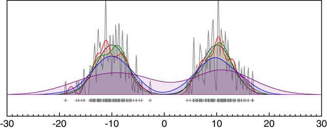
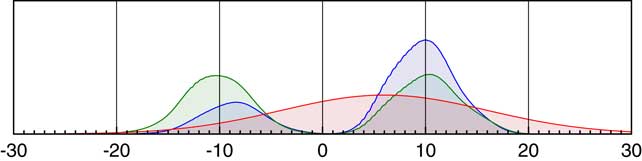
Because of the complication of 14C calibration, before discussing calibrated dates it is worth seeing how the summing procedure works in a much simpler situation. Figure 1 shows what happens if a series of measurements are made on samples selected from a bimodal normal distribution. We assume that these values are measured with a range of different uncertainties, thereby introducing noise. Normal probability distributions with a mean of the measured value and a standard deviation of the uncertainty are then summed. When the measurement uncertainty is small the summed distribution is a very poor representation of the underlying bimodal distribution, showing a lot of high frequency noise. At intermediate values there are spurious peaks, very similar to those frequently seen in summed 14C calibrations. When the uncertainty becomes higher the simple bimodal distribution is generated but smeared by the uncertainty. Only if the sample number is high and the uncertainty happens to have an appropriate value will the summed distribution give a reasonable indication of the distribution from which the samples have been taken.
The effect of using the summing of likelihood distributions for measurements with normally distributed errors. The black line shows a bimodal normal distribution (centers: ±10, standard deviations: 3.0) from which 100 random samples have been generated (shown in the rug plot). Each of the other curves shows what happens if these values are measured with different standard uncertainties (gray: 0.1, red: 0.5, green: 1.0, blue: 2.0; purple: 4.0) and then the normal distributions associated with the measurement likelihood summed. Even with this number of samples the distributions are very noisy unless the measurement uncertainty is large, at which point the original distribution is smeared and it is no longer possible to fully resolve the two original modes.
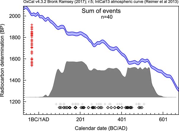
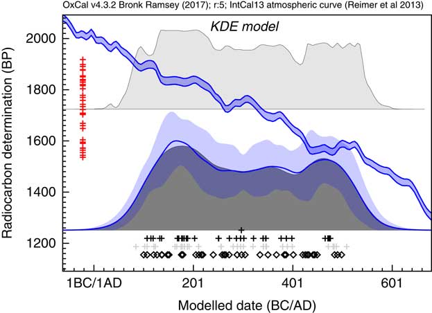
Sum distributions of 14C dates have exactly the same issues but in addition have the complication of the non-normal distributions from calibration. Figure 2 shows an example of a sum distribution exhibiting some of the common features: sharp drops and rises associated with features in the calibration curve and unrelated to the underlying distribution of events, and an excessive spread beyond the range from which the dates have been sampled, especially where there are plateaus in the calibration curve. This can be seen more clearly in Figure 3a where the Sum approach is compared to other methods. In general, there are three main problems with this as an approach: noise due to the limited number of dated samples, noise from the calibration process, and excessive spread due to measurement uncertainty.
An example of a sum distribution of calibrated 14C likelihood distributions. The open diamonds show the values of the randomly selected dates from the range AD100–AD500 for simulation, the red crosses on the left show the simulated 14C date central values (all errors in this case are ±25) and the light gray crosses below show the median values of the resulting calibrated likelihoods.
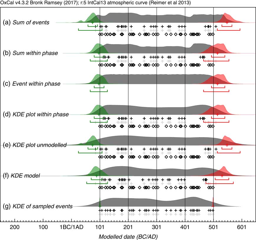
Comparison of methods of summarizing a set of 40 14C dates. The same simulations are used as in Figure 2. The open diamonds show the randomly selected dates in the range AD100–AD500, the light gray crosses show the medians of the likelihood distributions of the calibrated dates and the black crosses the medians of the marginal posterior distributions for each dated event. Panel (a) shows the sum of the likelihoods. Panels (b), (c), and (d) all use the marginal posteriors from the same simple single uniform phase model with a start and end boundary (Bronk Ramsey Reference Bronk Ramsey2009): panel (b) shows the sum of the marginal posteriors, panel (c) shows the marginal posterior for an event simply constrained to lie between the start and end boundary and panel (d) shows a Kernel Density plot based on the dated events constrained to be within the phase. Panel (e) is a KDE plot generated from samples randomly taken from the likelihood distributions. Panel (g) shows the effect of applying the KDE_Model model which uses the KDE distribution as a factor in the likelihood (see text). Panel (g) shows a Kernel Density plot of the original calendar dates chosen from the range AD100–AD500: ideally this is the distribution that the other estimates should reproduce. The overlain green and red distributions with their associated ranges show the marginal posterior for the First and Last events within the series: these should overlap at 95% with the first and last open diamonds which are the actual first and last events sampled; this is the case for those based on the uniform phase model, and the KDE model but not those based on the unconstrained Sum or KDE plot.
Sum Distributions within Models
If the processes underlying the data are properly understood, it is possible to overcome the excessive spread problem by employing a Bayesian model. Most simply a single uniform phase model might be used. It is then possible to calculate a Sum for the marginal posterior distributions of the events within the phase. This provides a visualization of the overall distribution of dated events within the phase. However, this still leaves the problem of the two types of noise due to calibration and the limited number of data-points. It is still very difficult to distinguish this noise from the signal (see Figure 3b).
Undated Events within Phases
A third approach can be used within a Bayesian phase model to produce a distribution which summarizes our knowledge of each phase inferred only from the boundary dates (see for example Loftus et al. Reference Loftus, Sealy and Lee-Thorp2016). We can postulate an undated event within the phase which obeys the priors (start and end boundaries, together with any particular phase distribution). This produces a smoother distribution (as shown in Figure 3) but it does not reflect the actual distribution of events for which there are date measurements. This can still, however, be a convenient way to summarize both boundary dates in a single plot.
Genetic Models
It is also possible to build other types of information into chronological models. Perhaps the best case is for demographic data with ancient DNA analysis. Ho and Shapiro (Reference Ho and Shapiro2011) is a useful review of methods employed including Bayesian multiple-change-point (MCP), Bayesian skyline, and Bayesian skyride. These all incorporate information on the way populations are likely to change over time, making the models both more precise and also more robust. Where 14C is used with these genetic models this has not usually been done with the full probability distribution function from calibration. Molak et al. (Reference Molak, Suchard, Ho, Beilman and Shapiro2015) have implemented such a procedure and found that, given the other uncertainties inherent in the genetic models, the output from the models is not usually affected.
KERNEL DENSITY PLOTS
One of the most widely used non-parametric methods for estimating underlying distributions of discrete data points is kernel density estimation (KDE; Rosenblatt Reference Rosenblatt1956; Parzen Reference Parzen1962). This is a frequentist rather than a Bayesian approach with no formal prior for the distribution. Effectively what the Sum distribution is generating is similar to a KDE distribution where the kernel is the probability distribution function from the calibration. This is not a suitable kernel for two reasons: firstly the width of the kernel is not optimized for the sample density, and secondly the kernel shape is strongly dependent on the details of the calibration process. This is why the Sum approach has the problems outlined above. However, it is still important to make use of the uncertainty associated with the calibration. To achieve this, it is possible to use a KDE approach for each specific MCMC state of the sampled distributions and average over the different MCMC states. For any particular set of events t={t 1 . . . t n }, assuming a normalized kernel distribution K(u), and a bandwidth h, the KDE estimate of the underlying distribution is given by:
 $$\hat{f}_{h} (t)\,{\equals}\,{1 \over {hn_{{}} }}\mathop{\sum}\limits_{i{\equals}1}^n {K\left( {{{t{\minus}t_{i} } \over h}} \right)} $$
Kernel Density Estimation Algorithm
Kernel choice and bandwidth estimation are the main issues when generating KDEs. The standardized normal kernel is widely used where K(u) ∼N(0,1), but other kernels might also be justified. In this application, the normal kernel will be used because of widespread use and known properties. Silverman’s rule (Silverman Reference Silverman1986) provides an optimal choice of bandwidth for use with normal kernels where the underlying distribution is assumed to be normal too. This estimate for the bandwidth is:
 $$h_{S} ({\bf{t}} )\,{\equals}\,(4\,/\,3)}^{{{1 \over 5}}} \hat{\sigma }({\bf{t}} )n^{{{\minus}{1 \over 5}}} $$
where σˆ is the sample standard deviation. This should be considered a maximum bandwidth as it usually over-smooths multi-modal distributions. In order to overcome this problem, the Silverman bandwidth can be multiplied by a shaping parameter g with a uniform prior:
 $$h({\bf{t}} )\,{\equals}\,gh_{S} ({\bf{t}} )$$
 $$g\sim{\!}\,U(0,1)$$
Effectively this allows the bandwidth to take any value with an upper limit of the Silverman estimate. The upper limit ensures that the Uniform prior is proper and also ensures that kernels are not considered which would be wider than optimal (this is only important because of the MCMC approach used below). A predictive likelihood can then be used to weight possible values of g. Here the predictive likelihood is taken to be:
 $${\cal L}\left( {{\bf{t}} \left| g \right.} \right)\propto\left[ {\prod\limits_{i\,{\equals}\,1}^n {\left( {{1 \over {\left( {n{\minus}1} \right)\,gh_{S} ({\bf{t}} )}}\mathop{\sum}\limits_{j{\equals}1,j\,\ne\,i}^n {K\left( {{{t_{i} {\minus}t_{j} } \over {gh_{S} (t)}}} \right)} } \right)} } \right]^{{(n{\minus}2)\,/\,n}} $$
where each element in the product is the likelihood of a single event as predicted by the KDE using all of the other events within the set. The power of (n−2)/n is used because once the mean and standard deviation are known there are only (n−2) degrees of freedom; it also follows that if n=2 there is no information available to determine the multi-modality of the KDE. For large n the power of (n−2)/n will make very little difference to the probability distribution. One approach would be to select g as the value that gives a maximum in the likelihood function (in which case the power applied would be irrelevant) as proposed for example by Zhang et al. (Reference Zhang, King and Hyndman2006). However, because the parameters t are themselves varying during the MCMC simulation, rather than for each pass find a maximum likelihood (which would be computationally expensive), the parameter g is included within the MCMC using the Metropolis-Hastings algorithm. The result of this approach is that the output is a likelihood weighted average of KDEs with slightly different bandwidths (which is why the upper limit of the Silverman bandwidth is significant: the maximum likelihood would always give a bandwidth lower than or equal the Silverman estimate anyway).
The MCMC implementation within OxCal works by generating an equal number of random samples from each of the events t i specified within the model within the kernel probability distribution function:
 $$\propto\,K\left( {{{t{\minus}t_{i} } \over h}} \right)$$
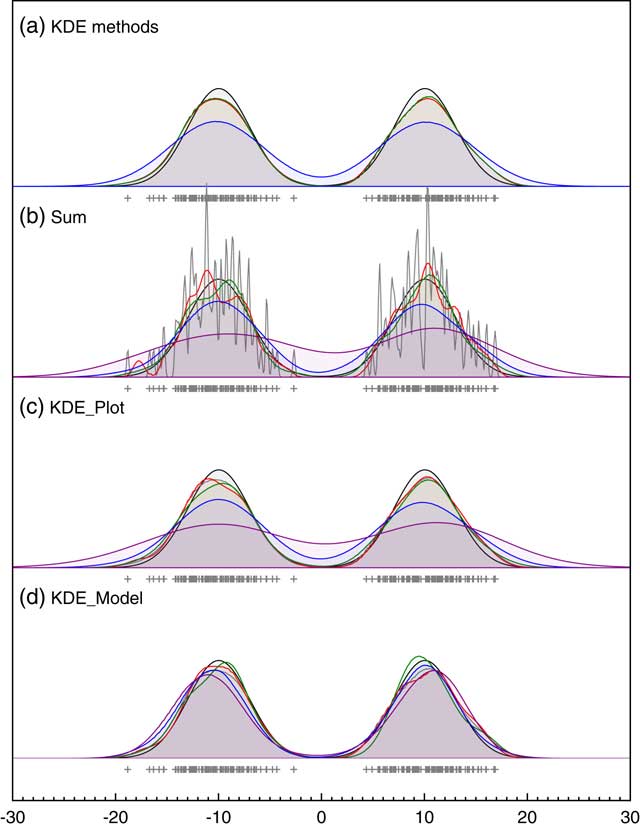
To test the effectiveness of this approach, it can be tested on data points with no uncertainty (the usual application of KDE) against the widely used Matlab KDE package which uses the more elaborate diffusion method of Botev et al. (Reference Botev, Grotowski and Kroese2010). Figure 4a shows that the outputs of the method presented here, and the diffusion method, are virtually indistinguishable (if anything this method is slightly closer to the original distribution) on two just resolvable normal distributions and both much better than Silverman’s rule on its own. The disadvantage of the method presented here for data with no uncertainty is that it is much slower since it involves MCMC. However, where MCMC is already being used to deal with uncertainty, the approach is faster than optimizing for each MCMC pass using an approach such as that of Botev et al. (Reference Botev, Grotowski and Kroese2010). It is also worth noting that, given there are many different methods for optimizing the choice of kernel width any KDE is just one possible estimate of the underlying frequency distribution and there is often no attempt to see how robust this is. The approach of using a Bayesian method and weighting for the likelihood rather than maximizing it, allows the family of plausible KDE distributions to be explored. The example given here shows that the mean of these distributions gives a result at least as close to the true distribution as other methods and furthermore gives some measure of robustness even in applications of KDE which do not involve measurement error.
Comparison of different approaches to KDE. Panel (a) shows the comparison of different methods for bandwidth estimation for data sampled from a bimodal normal distribution with centers at ±10 and standard deviation of 3; blue: Siverman-rule estimate, red: the MatLab KDE module (Botev et al. Reference Botev, Grotowski and Kroese2010) and green: the KDE_Plot method described here. Panel (b) is a repeat of Figure 1 showing the effect of changing measurement uncertainty (gray: 0.1, red: 0.5, green: 1.0, blue: 2.0; purple: 4.0) on the Sum distribution. Panel (c) shows the same for the KDE_Plot function on the same data. Panel (d) shows the application of the KDE_Model model implementation on the same dataset.
Implementation within OxCal
A new function KDE_Plot has been introduced into v4.3.2 of OxCal to provide KDE plots. The function takes three parameters:
 $${\tf="courier" KDE\_Plot}\,(name\;[,\;kernel\;[,\;factor]]);$$
where name is the label applied to the distribution, kernel is the kernel to be used (default is N(0,1)) and factor is the factor to be applied relative to the Siverman’s rule (default is U(0,1)). The command can either be used in place of the Phase function or be used as a query on any grouping and, in this respect, works in just the same way as the Sum function.
In addition to the sampling method used to generate the main KDE probability distribution, OxCal will also generate snapshots of the KDE during the MCMC at increments of 1000 iterations. An ensemble of these outputs can be plotted as shown in Figure 5 and the variability summarized as a blue band showing ±1σ. The ±1σ variability is useful as a summary but it should be remembered that this quantity will only be approximately normally distributed if the variability is small. If further detail is required on the variability, then the ensembles of possible KDE distributions should be further analyzed. In this particular case, the kernel width is well constrained and there is very little variation. An advantage of this MCMC approach is that this gives some indication of the robustness of the KDE to bandwidth selection.
This shows 30 individual KDE estimates generated during the MCMC with slightly different kernel bandwidths (based on the parameter g). The underlying data are as for Figure 4a. The blue line shows the mean of these and the light blue band ±1σ.
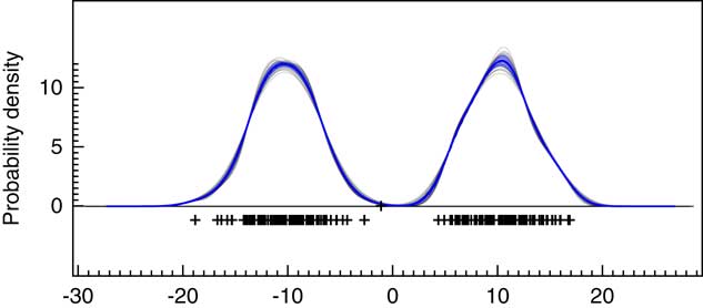
Figure 4c shows the output from the KDE_Plot algorithm for the same range of different measurement uncertainties as shown for the Sum function in Figure 1 (also shown in Figure 4b for comparison). Here it can be seen that the effect of the KDE is to eliminate the high-frequency noise seen in the Sum distributions where the measurement uncertainty is low. The approach does however smear the original signal when the uncertainty is higher (even slightly more so than the Sum). It is a conservative approach that is unlikely to reveal spurious structure.
Plots of Unstructured Chronological Data
The KDE_Plot algorithm can be tested on 14C datasets where Sum might have been used. Figure 3e shows the KDE plot for the same data which generated the summed plot shown in Figure 3a where the KDE estimate made on samples taken from the likelihood distributions. For reference the KDE of the calendar dates sampled is shown in Figure 3g.
This approach certainly does have advantages over using the Sum function in that the noise introduced from the calibration procedure is reduced (see Figure 3a). However, the KDE does not take any account of the dispersion in the data associated with the measurement uncertainty and if the First and Last events are sampled (see Figure 3e) these are the same as for the Sum method and too early and late respectively. In order to deal with this some other method is still required. If the data can be well represented by one of the existing Bayesian models (such as the uniform phase model) then it seems best to first use these to model the events listed in the model and then use KDE to estimate the distribution after modeling.
Kernel Density Plots within Bayesian Models
In the “Sum Distributions within Models” section, it was shown that the Sum can be carried out on the marginal posterior distributions instead of the likelihood distributions. We can do the same with the KDE_Plot function too. To do this, rather than simply sampling from the likelihood distributions a prior model such as the uniform model (Buck et al. Reference Buck, Litton and Smith1992; Bronk Ramsey Reference Bronk Ramsey2009) can be applied. In doing so the KDE distribution should also take account of the prior model being applied. This is in part achieved by by applying the prior to the t parameters in the model. However, this is not sufficient: the samples drawn within each kernel should obey the same prior (including boundary constraints). So if there is some prior (such as a uniform, normal or exponential distribution) which pertains to the events P(t) this can be used to modify the kernel shape for each point to:
 $$\propto\,P(t)\,K\left( {{{t{\minus}t_{i} } \over h}} \right)$$
where there is a hard boundary (a Boundary statement in OxCal) the kernel distributions are reflected at that boundary; this ensures that the distribution is uniform up to the boundary rather than rounding off. This enables abrupt transitions to be realistically handled by the KDE plotting routine. Note that equal numbers of samples are taken for the kernels associated with each t i to ensure that the actual distribution of events is still reflected in the final KDE. This has been implemented in OxCal so that the function KDE_Plot can be used within any model in the same way that the Sum function can. The effects of this can be seen in Figure 3d where the KDE plot generated within a modeled uniform phase better reflects the start and end of the phase than the unmodeled KDE plot (Figure 3e) and is still free of much of the high frequency noise in the Sum distribution (Figure 3a and b).
Overall this approach can be seen as a mixture of Bayesian and frequentist methods. The MCMC sampler uses the Bayesian likelihood and model priors and then for each sample state a frequentist KDE distribution is generated and averaged over the states. This mixture of statistical approaches is not unique: for example, Bayesian methods are often used to estimate the kernel bandwidth for KDE (Zhang et al. Reference Zhang, King and Hyndman2006). A Bayesian interpretation for the approach taken here would be that the prior for undated events is a product of the prior for the model and the (frequentist) KDE distribution generated for the dated events.
KERNEL DENSITY MODELS
From the discussion above it is clear that using the KDE_Plot method (Figures 4c and 3d) provides a display of the distribution of events which is free from the noise artifacts seen in Sum plots (Figures 4b and 3a). However, unless the plotting method is used together with another Bayesian model (Figure 3d), the distributions are over-dispersed (Figure 3d) and smear the underlying signal (Figure 4c). This is ultimately nothing to do with the method itself, it arises from the assumption that each parameter is totally independent and therefore a greater spread is statistically much more likely.
In many circumstances, it is incorrect to assume complete independence of our events: often the events form a coherent grouping, albeit perhaps with variations in event frequency. Consider the simple situation illustrated in Figure 4. Supposing of the 100 parameters sampled here, there are precise measurements for 99 of them. For the 100th parameter there might be no measurement information at all and then, if all of the parameters were entirely independent, the marginal posterior should be uniform across the entire parameter space. If on the other hand the parameter is from the same group as those for which there are 99 precise values, then it would be reasonable to assume that the 100th parameter likelihood could be defined by the distribution of the other 99 values. The best estimate for this distribution is given by the KDE. Alternatively, supposing for the 100th parameter there is a measurement but an imprecise one, for example 6±10. In this case, there is some more information: the measurement itself can define the likelihood but if the parameter is still part of the same group as the other 99, the KDE from our other values could still be used to narrow this down and, for example, down-weight the values around 0. What is required is for the likelihood to be given by the product of the likelihood from the measurement and the KDE from the other parameters as shown in Figure 6.
Schematic of likelihood for a parameter within a KDE model. If 99 parameters, all with precisely known values generate a bimodal KDE as shown in green, and the 100th parameter has a likelihood given by measurement of 6±10 as shown in red, then the combined likelihood for the true value of this 100th parameter is shown in blue.
In practical cases, all of the parameters to be modeled are like to have measurement uncertainty associated with them, but by using MCMC it is still possible to use the KDE associated with the values of all of the other parameters in the chain to define a KDE for updating any individual parameter. The weighting function to be applied to the likelihood is simply give by the factors of Equation 5:
 $$p(t_{i} \left| {g,{\bf{t}} _{{j\,\ne\,i}} } \right.)\propto\left( {{1 \over {(n{\minus}1)gh_{S} ({\bf{t}} )}}\mathop{\sum}\limits_{j{\equals}1,j\,\ne\,i}^n {K\left( {{{t_{i} {\minus}t_{j} } \over {gh_{S} ({\bf{t}} )}}} \right)} } \right)^{{(n{\minus}2)\,/\,n}} $$
The power of (n−2)/n is included here for two reasons. Firstly if there are less than three parameters, then it is not possible to estimate the bandwidth for a KDE. Secondly with this power, the probability of the model as a whole scales as ∝ σ2−n (t) (because hS ∝ σ(t)) and this means that the model is scale invariant because the statistical weight of the model with a span of s scales as s n−2 (Buck et al. Reference Buck, Litton and Smith1992; Bronk Ramsey Reference Bronk Ramsey2009). Like the uniform phase model, this KDE model should be able to deal with the excessive scatter due to statistical weight.
Although the KDE model probabilities are chosen to be scale invariant, unlike the parameterised models (Buck et al. Reference Buck, Litton and Smith1992; Bronk Ramsey Reference Bronk Ramsey2009), the effective prior for the span or standard deviation of these models is not necessarily uniform. For this reason, the Bayesian models with boundary parameters such as the uniform (Buck et al. Reference Buck, Litton and Smith1992; Bronk Ramsey Reference Bronk Ramsey2009) triangular, or normal (Bronk Ramsey Reference Bronk Ramsey2009) models would be more appropriate where this is something required of the model.
This overall approach for the KDE model is an extension to that used for the KDE_Plot where the KDE was used only to estimate the distribution of undated events. From a Bayesian perspective, the prior for each dated event is the KDE distribution for all of the other events, and the prior for all undated events is the KDE for all of the dated events. Because the KDE method is in itself frequentist, this is not a purely Bayesian approach. There may be other possible Bayesian methods such as the Bayesian Bootstrap (Rubin Reference Rubin1981) but none are without their problems and all require information on the distribution characteristics. If it is accepted that the KDE is a generally reasonable estimate for any underlying density when we have randomly selected samples, then the approach taken here is a reasonable approach for dealing with densities of events for which we have little or no quantitative prior knowledge.
Implementation in OxCal
The KDE_Model is implemented in OxCal and has a format:
 $${\tf="courier" KDE\_Model}\,(name\;[,\;kernel\;[,\;factor]])\left\{ {...} \right\};$$
where the events to be modeled are contained within the braces {...}. The kernel and factor default to N(0,1) and U(0,1) as for the KDE_Plot function above.
The MCMC algorithm allows for four different trial state changes:
-
∙ One event t i within the distribution is updated: the acceptance of this trial move depends on the product of the the KDE distribution probability given in Equation 9 for all of the other events, and the likelihood associated with any direct measurements on t i . See Figure 6 for a schematic explanation of how this works.
-
∙ The shaping parameter g is updated: acceptance of this move depends on the using the probability given in Equation 5. This is exactly the same step as is used in the KDE_Plot algorithm.
-
∙ All of the events t are shifted together: acceptance of this move depends only on the combined likelihoods of all of the parameters. All of the probabilities associated with the KDE model remain unchanged.
-
∙ All of the events t are expanded or contracted about the mean: acceptance of this move depends only on the combined likelihoods of the parameters; the change in phase space is balanced by the KDE model probability.
Both of the last two moves are only used to improve convergence in models with a very short overall span. For many applications, they are not necessary and could be omitted.
As with all MCMC Bayesian models implemented in OxCal, the Metropolis Hastings algorithm is used to decide whether to accept or reject trial moves (see for example Gilks et al. Reference Gilks, Richardson and Spiegelhalter1996). In the current version of OxCal the proposal distributions for dated events are uniform, covering the full possible range of the likelihood, and similarly that for the shaping parameter g is ~U(0,1), covering the full possible range. For the shift move a quite wide (±1σ) symmetrical uniform proposal distribution is used and for the expansion/contraction factor a log-uniform distribution ranging between 0.5 and 2. In general in OxCal bounded uniform rather than Gaussian proposal distributions are used because of the multi-modal nature of calibrated 14C likelihood distributions. Future versions may use adaptive sampling procedures depending on the context which might speed up convergence.
Tests on Simulated Data
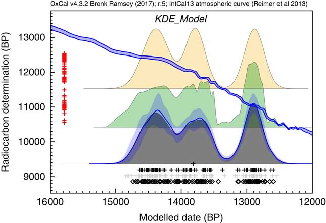
The KDE_Model algorithm can be tested against the same simulated uniformly distributed data that we used with the Sum method in Figure 2, as shown in Figure 7. The output of this model, together with the sampled distributions for the First and Last events is shown in Figure 3f where it can be seen that the overall span is much closer to the original, or to the output of the single uniform phase model (Figure 3b–d), than either the Sum plot (Figure 3a) or the KDE_Plot (Figure 3e). The algorithm removes high frequency noise in the form of sharp edges, peaks and troughs but does retain lower frequency signal. The method is not as good at detecting the abrupt ends to the true distribution as the uniform phase model which specifically assumes abrupt boundaries: this can be seen in the more sloping tails of the distribution and the the marginally wider estimates for the first and last event. The method does provide an output similar to that for the KDE plot for the randomly selected calendar events (Figure 3g) which is the objective of the method.
Plot showing the output of the KDE_Model method when used on the same simulated data as Sum in Figure 2. The open diamonds are a rug plot of the calendar date random samples, the light gray crosses show the medians of the likelihood distributions from the simulated 14C measurements for these dates and the black crosses show the medians of the marginal posterior distributions for the events from the KDE_Model analysis. On the left the rug plot for the central values of the simulated 14C dates is shown and the calibration curve is shown for reference. The dark gray distribution is the sampled KDE estimated distribution. The blue line and lighter blue band overlying this show the mean ±1σ for snapshots of the KDE distribution generated during the MCMC process and give an indication of the significance of any features. The light gray distribution shown above is the Sum distribution for reference.
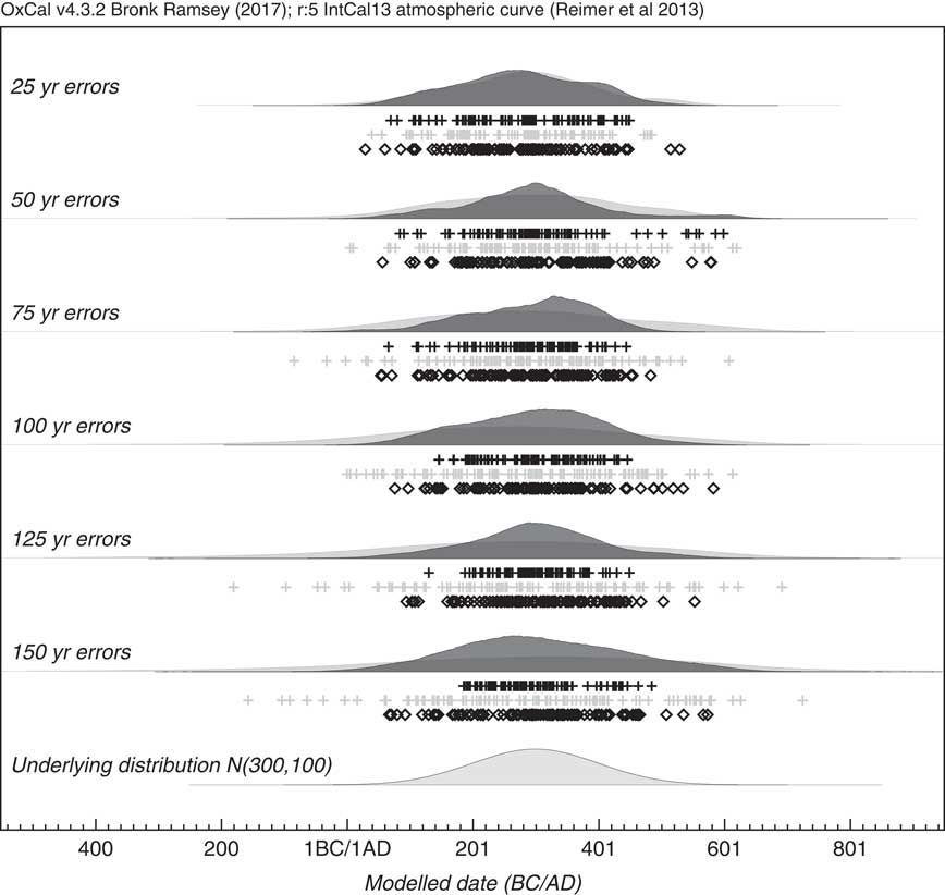
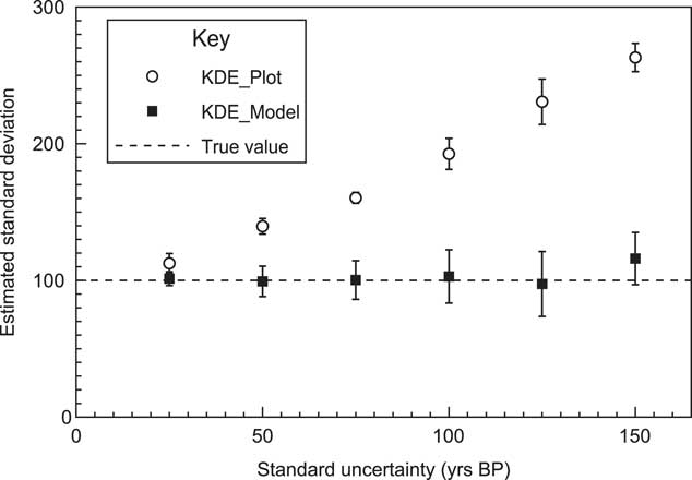
By looking at a simulated case where the underlying events are normally distributed, the method can be tested for a range of 14C measurement errors. Figure 8 shows an example of how a series of simulations with increasing uncertainty, still reproduces the original underlying distribution well. To test this further a series of 10 different simulations were done for the sample range with different uncertainties, and the results of the estimate for the standard deviation of the KDE distribution are shown in Figure 9. The estimated standard deviation remains correct and is, within errors, independent of the uncertainty. This contrasts with the approach of just using a KDE_Plot without any Bayesian model, which gives similar results to using a Sum distribution. In this case it can be seen that the KDE_Model is a good substitute for a parameterized normal distribution model.
Simulation of events with an underlying normal distribution N (300, 100). Each simulation has 100 events and assumes a different measurement uncertainty ranging from 25 to 150 yr. The light gray distributions show the effect of using KDE_Plot without any Bayesian modeling. The dark gray distributions are the output of a KDE model using the KDE_Model command within OxCal. The underlying distribution is shown for comparison. The rug plots show the randomly selected calendar dates (diamonds), the medians of the simulated 14C dates (light gray crosses) and the medians of the marginal posteriors of the simulated events (black crosses).
Details of the models used are explained in Figure 8. The estimated standard deviation of the underlying distribution is shown based on 10 different runs of each model with the error bars showing the sample standard deviation in results. The events are sampled from a normal distribution of 100. This plot shows that the KDE_Model algorithm recovers the underlying distribution independently of uncertainty whereas a simple KDE_Plot without a Bayesian model shows over-dispersion as the measurement uncertainties increase.
In the case of the kernel density model the power of (n−2)/n in Equation 9 is much more important than it was for KDE plots. Although in most instances where the spread of dates is considerable (including most examples given in the section “Example Applications of KDE Models”, with the exception of that for the British Bronze Age), a bias on the overall spread of dates proportional to s −1 or s −2 would be imperceptible, for models with short spans the impact would be considerable and the ability of the model to correctly determine the spread of dates as seen in Figures 8 and 9 would be compromised. Perhaps even more importantly the singularity at s = 0 would result in the MCMC becoming locked into states with very low span. With this power included, the MCMC is well-behaved and any bias in overall spread is avoided.
The real advantage in the approach comes with dealing with multi-modal distributions. Before considering 14C calibrated data it is worth testing the method on the simpler bimodal data shown in Figure 4. The KDE_Model algorithm has been applied to the same data with a range of uncertainties and associated noise added. The results of this analysis are shown in Figure 4d. The method successfully removes the high frequency noise seen in the Sum output and also eliminates the dispersion shown in the both the Sum and KDE_Plot distributions (Figure 4b and c). The method retains the lower frequency signal and removes the high frequency noise.
A final theoretical simulation is shown here for simulated 14C dates from the Late Glacial period. Figure 10 shows how the KDE_Model approach performs in comparison to the Sum distribution. In this case the KDE_Model performs much better at reproducing the underlying distribution of events without the sharp spikes and edges which characterize the Sum.
Two hundred dates were randomly sampled from a multimodal distribution. The events are assumed to be drawn from the trimodal distribution with modes centered on 14,400, 13,800, and 12,900 cal BP with standard deviations of 200, 150, and 150 respectively. There are 40 events in the first mode and 30 in the other two. The 14C measurements are assumed to have a standard error of 50 and measurement scatter has been simulated. The original underlying distribution is shown at the top, a simple Sum below that and the output of the KDE_Model algorithm outlined here. The rug plot is as for Figure 7.
EXAMPLE APPLICATIONS OF KDE MODELS
Here the KDE_Model methodology is tested on a number of published datasets in order to illustrate the ways in which it might be useful.
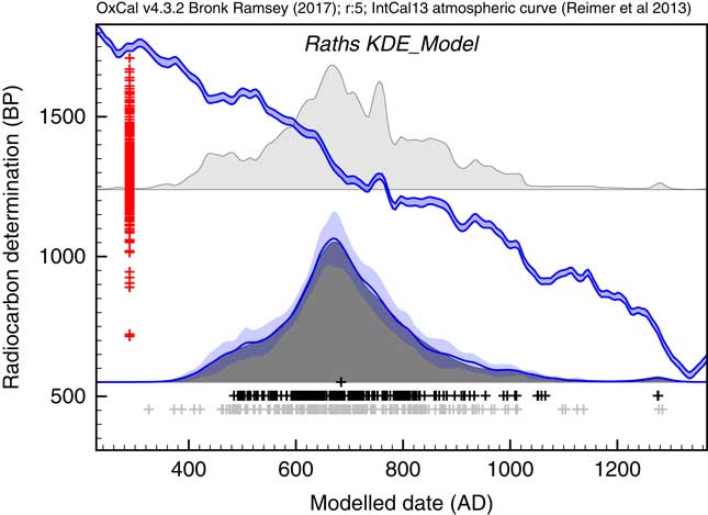
Irish Early Mediaeval Settlements (Raths)
The first application used the dataset of Kerr and McCormick (Reference Kerr and McCormick2014) on raths. Much of their paper is focused on how to deal with the artifacts in the distribution of raths through the early mediaeval period using a combination of binning and subtraction of probability distributions. They conclude that it is important not to over interpret the details of the distribution. Figure 11 shows the effect of using the KDE_Model function to summarize the data. This analysis would suggest that the material dated in the raths can be as old as the 5th and 6th centuries but that very little dates to later than about 1050. The exact interpretation would depend on issues of sample taphonomy beyond the scope of this paper. However, the key point is that here is no significant second peak in date density in the second half of the 8th century as suggested by the Sum distribution, and as concluded by Kerr and McCormick (Reference Kerr and McCormick2014).
Comparison of Sum distribution (above) and KDE_Model distribution for dates on raths as reported in Kerr and McCormick (Reference Kerr and McCormick2014). The features of the plot are the same as Figure 7.

British Bronze Age Axes
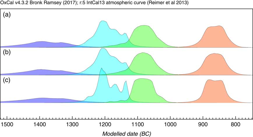
The next application is not ideally suited to the KDE_Model method because it is based on phased material with possibly quite short phase lengths, which can be better modeled using purely Bayesian parametric models. The dataset chosen for this is the same as that used to test the trapezium model in Lee and Bronk Ramsey (Reference Lee and Bronk Ramsey2012) which relates to dates on British Bronze Age axes (Needham et al. Reference Needham, Bronk Ramsey, Coombs, Cartwright and Pettitt1998). Here three different approaches to summarize the dates on each Bronze axe type are applied. The first method is to assume an underlying uniform phase model as used in the original publications (Needham et al. Reference Needham, Bronk Ramsey, Coombs, Cartwright and Pettitt1998) with a KDE_Plot to visualize the distribution; the second is to use a normal distribution for the data (Bronk Ramsey Reference Bronk Ramsey2009), and then use KDE_Plot to show the distribution of events; finally the KDE_Model is used on its own to both model and visualize the data. The results of these analysis options are shown in Figure 12. It is clear that all methods give very similar results. This data has a peculiarity in that for all of the groups other than Acton and Taunton, the dates are not statistically different from each other and so actually each group could be short-lived. Given this characteristic, the modeled spans of those phases are actually shorter with the KDE_Model which is just visible in the plots. Overall it is encouraging that the non-parametric KDE method gives such similar solutions in a unimodal case like this, though it is not recommended where the overall span might be close to zero or where a purely Bayesian parametric model can be used.
Comparison of methods for summarizing dates on different types of bronze axe from the British Bronze Age (data from Needham et al. Reference Needham, Bronk Ramsey, Coombs, Cartwright and Pettitt1998). The phases shown in all cases are from left to right: Acton and Taunton (5 dates), Penard (12 dates), Wilburton (10 dates), and Ewart Park (9 dates). Panel (a) shows the results of using independent (overlapping) single uniform phase models for each group with the probability distribution between the boundaries being visualized using KDE_Plot. Panel (b) shows the same but using a normally distributed phases (using Sigma_Boundary, see Bronk Ramsey Reference Bronk Ramsey2009). Panel (c) simply uses a KDE_Model for each group of dates. All methods give very similar results indicating that the Acton and Taunton, Penard and Wilburton phases follow on one after the other with a short gap before Ewart Park.
Paleoindian Demography
The next example draws on the dataset of Buchanan et al. (Reference Buchanan, Collard and Edinborough2008), also discussed by Culleton (Reference Culleton2008) and Bamforth and Grund (Reference Bamforth and Grund2012). Again much of the discussion arises out of what can be considered noise and what is signal in the summed distributions of calibrated 14C dates. Here the same dataset is analyzed using the KDE_Model algorithm. The results of this analysis are shown in Figure 13.
Comparison of Sum distribution (above) and KDE_Model distribution for dates on Paleoindian contexts as reported in Buchanan et al. (Reference Buchanan, Collard and Edinborough2008). The features of the plot are the same as Figure 7.

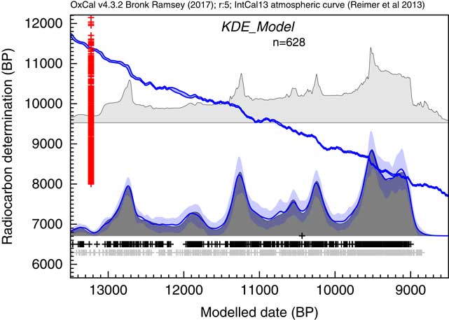
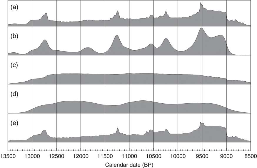
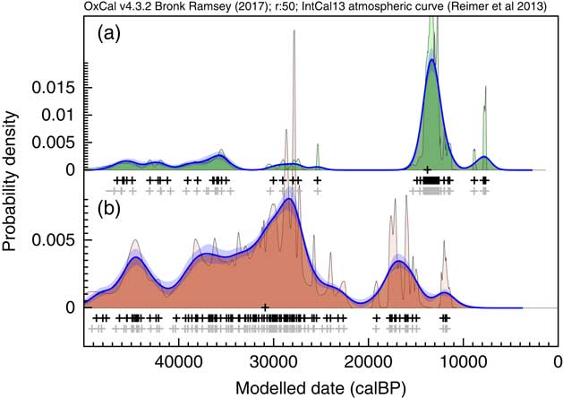
This analysis would suggest that there is a useful signal in the original data but that it is somewhat masked by the Sum distribution. It has been pointed out that simulations will show fluctuations even if the underlying density of dates is uniform. This is true, and this is not entirely due to the calibration curve either, it is simply a result of stochastic noise. In order to explore this further, like Bamforth and Grund (Reference Bamforth and Grund2012), a simulation of 628 14C dates with comparable error terms has been undertaken over a similar time period (12,950–8950 cal BP) uniformly distributed throughout the period. These simulated dates have then been summed (as shown in Figure 14c) and subjected to the same KDE_Model analysis. The results of this analysis are shown in Figure 14d.
Comparison of different distributions related to the data from Buchanan et al. (Reference Buchanan, Collard and Edinborough2008) (628 dates). Panel (a) shows the simple Sum distribution; panel (b) is the KDE_Model analysis as shown in Figure 13; panel (c) shows the Sum distribution from the simulation of 628 dates uniformly spread through the period 12,950–8950 cal BP; panel (d) shows the KDE_Model analysis of the same simulated dataset; panel (e) shows the simple Sum plot for dates simulated from the medians of the marginal posterior distributions arising from the KDE_Model analysis. The fact that panel (e) is similar to panel a indicates that the original sum distribution is compatible with the output of the KDE_Model analysis.

Although there are some underlying fluctuations in rate (which vary with each simulation) there are no obvious artifacts. As a final test of the method, the median marginal posterior dates from the KDE_Model have been taken as the true dates of the samples and a simulation run to recover the original Sum distribution. This is shown in Figure 14e and is very similar to the original Sum shown in Figure 14a. Each simulation will give slightly different results and the minor details are clearly not significant. One, albeit impractical, approach to analyzing a dataset like this would be to try a very large number of possible distributions, simulate the dates from them and see how well you could reproduce the original Sum distribution. Effectively this is what the KDE_Model analysis is achieving this case.
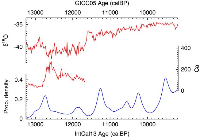
The results of the analysis can then be compared to the climate record of NGRIP (Andersen et al. Reference Andersen, Azuma, Barnola, Bigler, Biscaye, Caillon, Chappellaz, Clausen, Dahl-Jensen and Fischer2004; Bigler Reference Bigler2004; Rasmussen et al. Reference Rasmussen, Andersen, Svensson, Steffensen, Vinther, Clausen, Siggaard-Andersen, Johnsen, Larsen, Dahl-Jensen, Bigler, R̈othlisberger, Fischer, Goto-Azuma, Hansson and Ruth2006; Svensson et al. Reference Svensson, Andersen, Bigler, Clausen, Dahl-Jensen, Davies, Johnsen, Muscheler, Parrenin and Rasmussen2008) as shown in Figure 15. To return to the original subject of Buchanan et al. (Reference Buchanan, Collard and Edinborough2008), there is certainly no indication of an abrupt bottleneck at 12,900 cal BP: it would seem that the date density peaks slightly after that and then declines most rapidly as the Calcium flux in Greenland reaches its peak. Overall the data would suggest that there might be an interesting phase delay between what is recorded in NGRIP and the archaeological activity in North America.
A plot of the Ca flux and δ18O isotope ratios recorded in NGRIP (Andersen et al. Reference Andersen, Azuma, Barnola, Bigler, Biscaye, Caillon, Chappellaz, Clausen, Dahl-Jensen and Fischer2004; Bigler Reference Bigler2004; Rasmussen et al. Reference Rasmussen, Andersen, Svensson, Steffensen, Vinther, Clausen, Siggaard-Andersen, Johnsen, Larsen, Dahl-Jensen, Bigler, R̈othlisberger, Fischer, Goto-Azuma, Hansson and Ruth2006; Svensson et al. Reference Svensson, Andersen, Bigler, Clausen, Dahl-Jensen, Davies, Johnsen, Muscheler, Parrenin and Rasmussen2008) against the KDE_Model derived probability density for dates from Paleoindian contexts in North America using data from Buchanan et al. (Reference Buchanan, Collard and Edinborough2008).
Megafauna in the Late Quaternary
The next datasets to be considered cover almost the entire range of the calibration curve. These are datasets for Megaloceros giganteus (Stuart et al. Reference Stuart, Kosintsev, Higham and Lister2004) and Mammuthus primigenius (Ukkonen et al. Reference Ukkonen, Aaris-Sørensen, Arppe, Clark, Daugnora, Lister, Lõugas, Seppa, Sommer and Stuart2011). The raw data in each case, over such a long timescale inevitably show considerable noise when viewed as a Sum distribution. The KDE_Model distributions (Figure 16) provide a much more reasonable starting-point for discussion of the underlying trends. Of course it is still very important to keep in mind sampling and survival biases which might affect these distributions but having a reasonable estimate for the distribution of dated specimens is still very useful.
KDE analysis of two sets of megafauna data from (a) Stuart et al. (Reference Stuart, Kosintsev, Higham and Lister2004) (77 dates on Megaloceros giganteus) and (b) Ukkonen et al. (Reference Ukkonen, Aaris-Sørensen, Arppe, Clark, Daugnora, Lister, Lõugas, Seppa, Sommer and Stuart2011) (112 dates on Mammuthus primigenius, excluding one beyond calibration range). In each case the rug plots show in light gray the median likelihoods of the calibrated dates, and in black the median of the marginal posterior distributions. The main KDE_Model distributions are shown in a darker shade with the much noisier Sum shown in the background. The blue lines and bands show the mean and ±1σ of the ensembles of snapshot KDE distributions from the MCMC analysis, showing in this case that the distributions are fairly well constrained.
Demography of Prehistoric Ireland
The final example provides a challenge to the methodology. The dataset is that used to discuss the end of the Bronze Age in Ireland in Armit et al. (Reference Armit, Swindles, Becker, Plunkett and Blaauw2014). This comprises 2020 14C dates (3 having been discarded because of insufficient information). This is challenging for the KDE_Model because Equation 9 entails relating the position of every event to every other event at each iteration. This becomes very slow for large datasets. For this dataset on a MacBook Pro (2.3 GHz Intel Core i7) it runs at about 1800 iterations (of all parameters) per hour. Ideally for a proper study this should be run for several days to ensure full convergence.
A purely practical point should be made about running models of this size. These are too large to run on the online OxCal server and even on a dedicated computer running through the web-interface may cause memory problems. It is recommended that the model be saved and then run from the command line of the operating system. To terminate the run delete the .work file and wait for completion and output of the results which may take some minutes. In future, it may be possible to optimize the algorithm further for such large models since in practice only near neighbor events really affect the KDE distribution significantly. However, it is useful to know that models with thousands of events are possible and the algorithm, although slow, still works well with reasonably rapid convergence for the main KDE distribution.
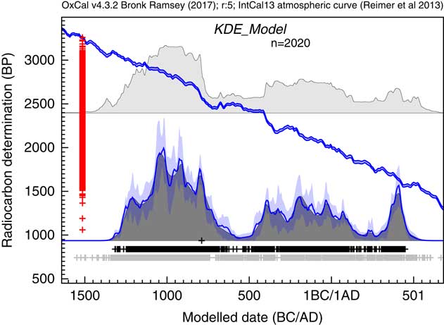
The output of the analysis is shown in Figure 17. The focus of the original study was the end of the Bronze Age in this region. The KDE analysis suggests a peak in density of dates at around 1050 BC with some fluctuation over the next three centuries to 750 BC. There is then a rapid fall, staring from a peak at about 800BC with very low density from 600 to 450 BC, consistent with the paucity of evidence for the Early Iron Age (Armit et al. Reference Armit, Swindles, Becker, Plunkett and Blaauw2014). The KDE analysis would suggest that this fall, is actually underestimated in the Sum distribution because the calibrated ranges for dates on either side of this range extend right across this period.
Comparison of Sum distribution (above) and KDE_Model distribution for dates on Irish archaeological sites in the period 1200 BC to AD 400 as reported in Armit et al. (Reference Armit, Swindles, Becker, Plunkett and Blaauw2014). The features of the plot are the same as Figure 7.
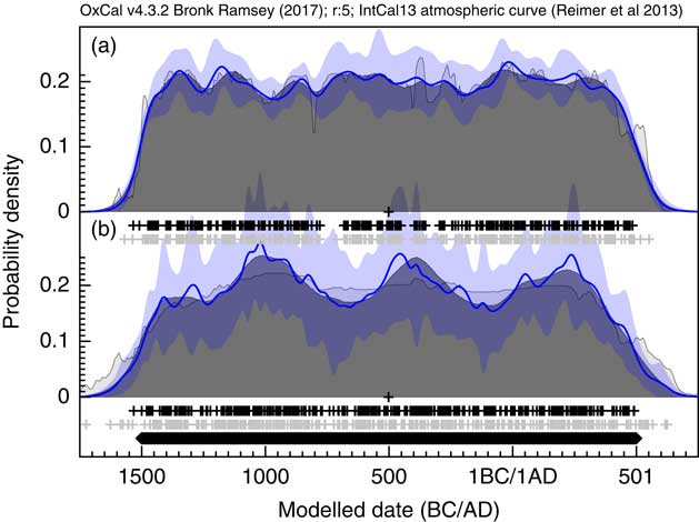
A legitimate question would be whether the drop in density seen in the Early Iron Age could be due to the calibration plateau covering roughly 800–400 BC. One aspect of this can be tackled by simulation. Multiple simulations through this period do not show any consistent patterns, although the models do often show more variability through this period. A couple of examples of simulations with uniform density are shown in Figure 18 and although patterns are visible they are generally consistent with a uniform density if you take into account the variability in the snapshot KDE distributions. This variability is greater if the error margin on the dates is larger as is to be expected. However, the drop seen in Figure 17 would seem to be unambiguous. Of course there is always the issue of sampling bias to consider and in general there is a tendency not to 14C date Iron Age material because of the 14C plateau which could have a very significant effect on such a study. Whether this is the case or not in Ireland is a question beyond the scope of this paper.
Example simulations of 400 14C dates on uniformly distributed events through the period 1500 BC to AD 500. The uncertainty of the dates is assumed to be ±30 and ±100 14C yr in panels (a) and (b) respectively. The blue bands show the ±1σ variability in snapshot KDE distributions generated during the MCMC analysis with more uncertainty seen in panel (b) (±100) than in panel a (±30). There is no consistent patterning in where rises and falls in the distribution occur and these are therefore consistent with stochastic effects of the simulations.
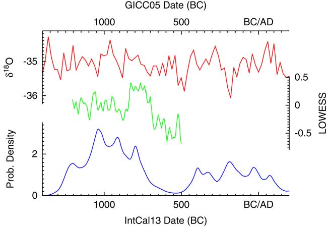
Having generated a density of dates, this can then be compared to the climate data as presented in Armit et al. (Reference Armit, Swindles, Becker, Plunkett and Blaauw2014). Figure 19 shows the density plotted both against the NGRIP δ18O isotope record (Andersen et al. Reference Andersen, Azuma, Barnola, Bigler, Biscaye, Caillon, Chappellaz, Clausen, Dahl-Jensen and Fischer2004; Rasmussen et al. Reference Rasmussen, Andersen, Svensson, Steffensen, Vinther, Clausen, Siggaard-Andersen, Johnsen, Larsen, Dahl-Jensen, Bigler, R̈othlisberger, Fischer, Goto-Azuma, Hansson and Ruth2006; Svensson et al. Reference Svensson, Andersen, Bigler, Clausen, Dahl-Jensen, Davies, Johnsen, Muscheler, Parrenin and Rasmussen2008) and the climate summary statistic using LOWESS models (smooth = 0.02) presented in Armit et al. (Reference Armit, Swindles, Becker, Plunkett and Blaauw2014). This plot confirms the conclusions of Armit et al. (Reference Armit, Swindles, Becker, Plunkett and Blaauw2014) that the drop in date density actually proceeds the climatic downturn of the mid-eighth century. In addition, the finer structure of the KDE_Model analysis does seem to show some correlation in the period 1100–700 BC with the LOWESS curve with a slight lag, perhaps of the order of a generation or two. This could imply that demographics is partly being driven by climate during the later Neolithic, which would not be surprising.
Plot showing the probability density from the KDE_Model analysis of archaeological 14C dates from Ireland as summarized in Armit et al. (Reference Armit, Swindles, Becker, Plunkett and Blaauw2014) compared to the δ18O isotope record of NGRIP (Andersen et al. Reference Andersen, Azuma, Barnola, Bigler, Biscaye, Caillon, Chappellaz, Clausen, Dahl-Jensen and Fischer2004; Rasmussen et al. Reference Rasmussen, Andersen, Svensson, Steffensen, Vinther, Clausen, Siggaard-Andersen, Johnsen, Larsen, Dahl-Jensen, Bigler, R̈othlisberger, Fischer, Goto-Azuma, Hansson and Ruth2006; Svensson et al. Reference Svensson, Andersen, Bigler, Clausen, Dahl-Jensen, Davies, Johnsen, Muscheler, Parrenin and Rasmussen2008) and the LOWESS (smooth 0.02) climate analysis of Armit et al. (Reference Armit, Swindles, Becker, Plunkett and Blaauw2014). The NGRIP data is on the GICC05 timescale, all other data is based on 14C and so on the IntCal13 timescale (Reimer et al. Reference Reimer, Bard, Bayliss, Beck, Blackwell, Bronk Ramsey, Grootes, Guilderson, Haflidason, Hajdas, Hatte, Heaton, Hoffmann, Hogg, Hughen, Kaiser, Kromer, Manning, Niu, Reimer, Richards, Scott, Southon, Staff, Turney and van der Plicht2013). See text for discussion.
Discussion
These examples show the way in which the KDE_Model works in practice with real data. The ±1σ variability is useful in assessing the success in each case but additional information can be gained by looking at the marginal posterior distributions for the g shaping parameter because this is indicative of the nature of the distribution.
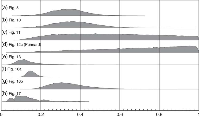
Figure 20 shows the marginal posteriors for g for a number of the examples of KDE_Model use throughout this paper. In general, the marginal posteriors have an approximately normal distribution (Figures 20a, b, e, f, g) and are quite different to the prior. If you look at the associated KDE distributions in these cases the ±1σ variability is also well behaved (low in magnitude and without major fluctuations). However, there are some interesting exceptions.
Marginal posterior distributions for the parameter g in applications of the KDE_Model for (a) the simulated bimodal distribution shown in Figure 5, (b) the simulated multimodal distribution shown in Figure 10, (c) the Irish early mediaeval settlements example from Kerr and McCormick (Reference Kerr and McCormick2014) shown in Figure 11, (d) the Pennard phase from the British Bronze Age data of Needham et al. (Reference Needham, Bronk Ramsey, Coombs, Cartwright and Pettitt1998) as shown in Figure 12c, (e) the Paleoindian contexts of Buchanan et al. (Reference Buchanan, Collard and Edinborough2008) as shown in Figure 13, (f) the Megaloceros giganteus data of Stuart et al. (Reference Stuart, Kosintsev, Higham and Lister2004) as shown in Figure 16a, (g) the Mammuthus primigenius data of Ukkonen et al. (Reference Ukkonen, Aaris-Sørensen, Arppe, Clark, Daugnora, Lister, Lõugas, Seppa, Sommer and Stuart2011) in Figure 16b, and (h) the data of Armit et al. (Reference Armit, Swindles, Becker, Plunkett and Blaauw2014) as shown in Figure 17. The model is most likely to be robust when the marginal posterior is a well defined, approximately normal distribution. If the mode is close to 1 (as in panel (d), a single phase parameterized Bayesian model would be more appropriate. This parameter should be assessed in combination with the variability in output results as seen either in ensembles of outputs or in the plot of the ±1σ variability.
The g parameter for the analysis of Irish early mediaeval settlements (Figure 11; Kerr and McCormick Reference Kerr and McCormick2014) is shown in Figure 20c. In this case g is not very well constrained although the maximum likelihood is around 0.4 so suggesting a non-Gaussian distribution. On the other hand, in this case the ±1σ variability in the KDE_Model is fairly low suggesting that the output of the model is just not very sensitive the choice of kernel width. What you do see is some fluctuation in the ±1σ variability which is associated with this lack of constraint in g. In this case, the model still seems to be useful and robust despite the lack of constraint on g.
In the British Bronze Age example (Needham et al. Reference Needham, Bronk Ramsey, Coombs, Cartwright and Pettitt1998), it has already been noted that the data for each phase is such that each phase could be very short. All of the marginal posteriors for g parameters for the different phases are similar and that for the Pennard type is shown in Figure 20d. The maximum likelihood for g occurs close to 1 indicating that the Silverman’s rule (Silverman Reference Silverman1986) estimate for the kernel is the most appropriate. This is in turn indicative of a unimodal distribution which can be well approximated with a normal distribution. The ±1σ variability is also larger than the mean value showing that the result is not robust. In this case clearly one of the parameterized Bayesian models would be much more appropriate.
Finally, the demography of prehistoric Ireland example (Figure 17; Armit et al. Reference Armit, Swindles, Becker, Plunkett and Blaauw2014) has a marginal posterior for the g parameter as shown in Figure 20h. This is reasonably well constrained but multimodal indicating that there are a number of different possible kernel widths that might be most appropriate. This is also reflected in the ±1σ variability visible in Figure 17, which exhibits fluctuations through time. It is clear that some of the fine structure here might not be significant.
In general, the ±1σ variability is a good guide to how robust the output is and the marginal posterior for g can indicate what the reasons for excessive variability are. In particular, if the mode marginal posterior for g is close to 1 then a parameterized Bayesian single phase model of some kind would be much more appropriate. Studying the marginal posterior for g also shows one of the strengths in approach of allowing g to vary in that multimodal distributions would be missed if a maximum likelihood method had been employed, giving an over-precise assessment of the underlying distribution.
CONCLUSIONS
There are a number of different methods available for the analysis and summary of 14C datasets. Where prior information is available on the nature of the datasets and their expected distribution, parametric Bayesian modeling has been found to be very useful. In such cases KDE plots can be used to summarize the distribution of events within such groupings in way which both retains signal and suppresses noise.
In a very large number of cases, however, the distribution of events is not well understood and yet parametric Bayesian analysis requires the assumption of a particular distribution in order to deal with the problem of over-dispersion from measurement error. Here it is shown that KDE modeling is a simple and widely applicable method that can be used in such circumstances. It allows for multimodality in the data and is seen to be much better in recovering underlying signal than other methods tested. The ability to assess the robustness of the KDE distributions by looking at the variability seen in distributions during MCMC analysis is also an important advantage over other methods such as summing which can only provide a single solution.
The KDE approach presented here is a simple one, based on kernels which have the same width throughout the distribution. There might well be other KDE approaches which could further refine this method. However, a simple approach has the advantage of keeping the underlying assumptions clear. The case studies presented here indicate that the method in its current form could be applicable to a wide range of important research topics.
In the introduction, it was pointed out that taphonomic issues are often very important in understanding large 14C datasets and it is important to remember that these cannot be eliminated using the statistical methods described here. In all cases the distributions generated are estimates for the distributions of the events which have been subjected to the filtering processes of survival and sampling. In some cases, it might be argued that survival and sampling is fairly random and that this does indeed give a reasonable representation of the original underlying processes. In most cases this will not be the case and further interpretation is required. However, even in these cases having a good representation of distribution of the events which have passed through the survival and sampling process is still a significant advance.
ACKNOWLEDGMENTS
All calibrations in this paper have been carried out using IntCal13 (Reimer et al. Reference Reimer, Bard, Bayliss, Beck, Blackwell, Bronk Ramsey, Grootes, Guilderson, Haflidason, Hajdas, Hatte, Heaton, Hoffmann, Hogg, Hughen, Kaiser, Kromer, Manning, Niu, Reimer, Richards, Scott, Southon, Staff, Turney and van der Plicht2013). The author would like to acknowledge support from the UK Natural Environment Research Council (NERC) for the Oxford node of the national NERC Radiocarbon facility.