



INTRODUCTION
Within-field and sub-field soil variability is a ubiquitous feature, management-induced (i.e., soil amendments) or the result of naturally occurring sources (Adamchuk et al., Reference Adamchuk, Ferguson, Hergert, Oerke, Gerhards, Menz and Sikora2010). Some soil properties exhibit highly dynamic characteristics varying rapidly with time and over distances ranging from mm to m, e.g., nitrate, temperature, moisture, microbial activity, water-soluble salts, nutrient concentration in soil solution and redox potential (Adamchuk et al., Reference Adamchuk, Ferguson, Hergert, Oerke, Gerhards, Menz and Sikora2010; Becker, Reference Becker1995; Dhillon et al., Reference Dhillon, Samra, Sadana and Nielsen1994; Lascano and Hatfield, Reference Lascano and Hatfield1992; Wierenga et al., Reference Wierenga, Hills and Hudson1991). Berndtsson and Bahri (Reference Berndtsson and Bahri1995) found that field variability of different element concentrations in plants can only partially be explained by corresponding soil variability. Spatial heterogeneity, reflecting the acquired part of the plant-to-plant variability, is owed to soil variation and inflated by uneven seed emergence, effects of clouds and capping in wet soils, uneven application of applied inputs, differential effects of herbivores, parasites or pathogens and interactions among these factors (Fasoula and Tokatlidis, Reference Fasoula and Tokatlidis2012). Acquired variability can have serious effects on the interpretation of variety trials, preventing precise distinction of the genotypes’ characteristics (Ball et al., Reference Ball, Mulla and Konzak1993; Brownie et al., Reference Brownie, Bowman and Burton1993; Stroup et al., Reference Stroup, Baenziger and Mulitze1994; Vollmann et al., Reference Vollmann, Winkler, Fritz, Grausgruber and Ruckenbauer2000).
Several techniques have been proposed for dealing with spatial heterogeneity in breeding field trials. The most common is the RCB design, where plots (PLs) are positioned on the basis of blocking and randomization within each block, as well as on replication of the blocks. The statistical validity of the RCB and accurate estimates depend primarily on the assumption that treatments are evaluated with respect to similar environmental and operational conditions within a block (Brownie et al., Reference Brownie, Bowman and Burton1993; Gusmao, Reference Gusmao1986). Papadakis (Reference Papadakis1937) was the first to propose the use of yield residuals from neighbouring PLs and paved the way for what is now termed NN analysis (Scharf and Alley, Reference Scharf and Alley1993). Assuming that close neighbours share a common micro-environment, the NN adjustment can improve both the precision and accuracy of field experiments (Magnussen, Reference Magnussen1993). Papadakis's idea motivated Briggs and Shebeski (Reference Briggs and Shebeski1968) to suggest unreplicated PLs with every third PL planted with a common control genotype (the check-PL method). However, the check-PL technique can still induce additional spatial heterogeneity because of the extra 33% of land required. Knott (Reference Knott1972) introduced the moving average method in which the mean of a number of adjacent PLs is used as a covariate for adjusting PL values, eliminating the need to devote PLs to checks. In the moving average procedure, however, the absence of common control genotype implies a varying baseline for PL adjustment. The lattice design (LD) suggested by Yates (Reference Yates1936) allows sampling of spatial variation in two directions (row–column); however, it is restrictive for the number of treatments and the field layout (Rosielle, Reference Rosielle1980). The honeycomb breeding methodology and respective experimental selection designs, i.e., HD, have been suggested as remedy for the confounding effects of spatial heterogeneity (Fasoula and Fasoula, Reference Fasoula and Fasoula2000; Fasoula and Tokatlidis, Reference Fasoula and Tokatlidis2012; Fasoulas, Reference Fasoulas1987, Reference Fasoulas1993; Fasoulas and Fasoula, Reference Fasoulas and Fasoula1995). Two inviolable rules obtain: individual plants grown widely apart to ensure the absence of competition and consideration of each plant as the experimental unit rather than the classical PL. Further, it has been asserted that advanced features of systematic instead of random entry allocation, plus multiple replications, ensure the highest efficiency in terms of sampling spatial heterogeneity and counteracting its detrimental effects on selection efficiency. Precise entry allocation enables adjustment on the same baseline, even if extra control is absent. In order to obtain the systematic arrangement for a given number of entries, a constant (k) value should be used so as to define the starting codes of each row (Fasoulas and Fasoula, Reference Fasoulas and Fasoula1995). For certain designs, the standardized pattern is accomplishable only if the set of entries is split into more than one row, called ‘grouped’ designs. For the rest (‘ungrouped’ designs), systematic arrangement is formed with entire sets of entries in each row. Numerous breeding studies have successfully incorporated this method, on two of which the present study was based (Tokatlidis, Reference Tokatlidis2000; Tokatlidis et al., Reference Tokatlidis, Xynias, Tsialtas and Papadopoulos2006).
Even though spatial heterogeneity can limit precise distinction of performance differences, breeders are reluctant to use elaborate statistical designs (e.g., lattice or NN adjustment designs), sustaining lower breeding efficiency (Ball et al., Reference Ball, Mulla and Konzak1993). Because of low densities, HDs demand considerably increased field areas, so the way they manage spatial heterogeneity is challenging. This paper considers the effectiveness of the systematic entry arrangement of the honeycomb pattern to correct for the effects of spatial heterogeneity of breeding field trials, and compares it with the classical RCB design, the NN analysis method and the LD. To appraise these procedures, two field trials were held.
MATERIALS AND METHODS
In trials including a mono-genotypic population, the coefficient of variation (CV) represents absolute environmental effects, depicting the level of spatial heterogeneity. Spatial heterogeneity is also depicted by the top-to-bottom gap (TBG) among the means of a number of simulated entries dispersed across the whole experimental area, as well as by the number of means significantly differing (MSD) from the overall (grand) experimental mean. Hereafter, the terms ‘significant residual’ and ‘mean deviating’ imply the statistically significant difference of an entry mean from the grand mean. The TBG was computed as a percentage of the overall trial mean. For example, assuming the value of 100 as grand mean, the entry mean range of 75–130 corresponds to +30 and −25% top and bottom deviation, respectively, thus to 55% TBG. The deflation in TBG obtained by an experimental technique was seen as reflecting its effectiveness in overcoming spatial heterogeneity. Data from two field studies pertaining to grain yield of individual plants were used to test the above hypothesis. The first comprised the maize (Zea mays L.) hybrid ‘B73xMo17’ (Tokatlidis, Reference Tokatlidis2000), and the second, the wheat (Triticum aestivum L.) cultivar ‘Nestos’ (Tokatlidis et al., Reference Tokatlidis, Xynias, Tsialtas and Papadopoulos2006). However, the maize trial was the primary source because its experimental area was more than three times larger and it had three additional agronomic traits (plant height, ear height, ear length).
The trial of the maize hybrid ‘B73xMo17’
The trial area was 44 m long and 77 m wide including 70 rows of 35 single-plant hills, i.e., 2450 hills in total. To construct the uniformity map, the procedure described in Petersen (Reference Petersen1994) was applied, smoothed in two directions. By omitting an edge plant of each row (because of the zig-zag arrangement, the first for the odd rows and the last for the even rows), the trial was divided into units of four (2×2) plants and their average corrected yield was recorded: it comprised 35 rows of 17 means on each row, i.e., 595 yield PLs. The running median of three PLs was used whereby the yield of a PL was replaced by the median of the three adjacent PLs on the same row or the same column. Finally, areas of equal yield were delineated (Figure 1).
Smoothed variability map constructed on the single-plant grain yield (g) from the uniformity trial of the maize hybrid B73xMo17. The coloured legend on the right gives the yield range of small plot units (g) corresponding to the respective delineated area. The whole area is divided into 28 square plots, with mean yield (g) and CVsp(%) of single plants shown in parentheses in the plot centre (the PL28 arrangement of Table 1), averaged lengthwise and breadthwise outside the trial borders. The within-circle numbers represent the best scenario of randomization of seven entries into four complete blocks (I–IV) corresponding to the RCB7b of Table 1. The table below the map depicts the plot yields of eight simulated entries replicated in four blocks either lengthwise (RCB8ln) or breadthwise (RCB8br). The above the map results of mean yield ( $\bar x$
), CVsp, and top-to-bottom gap (TBG) relate to seven simulated entries analysed as honeycomb layout (HD7) in three equal parts, with each frame corresponding to the part below it.
$\bar x$
), CVsp, and top-to-bottom gap (TBG) relate to seven simulated entries analysed as honeycomb layout (HD7) in three equal parts, with each frame corresponding to the part below it.

The influence of spatial heterogeneity on single-plant performance of the maize hybrid B73xMo17 for four traits, as illustrated by the range of mean values, the top-to-bottom gap (TBG) in relation to the overall mean and the number of means significantly differing from the grand mean (MSD), when the trial is divided into a number of plots (i.e., 28 for PL28), as well as the degree of amelioration if the respective simulated entries are allocated according to the randomized complete block (RCB) of four replicates or the ‘nearest-neighbour’ (NN) configuration or the lattice design (LD) pattern. The overall measures of mean value $(\bar x)$
, coefficient of variation of single plants (CVsp), and number of plants (n) are also given.
$(\bar x)$
, coefficient of variation of single plants (CVsp), and number of plants (n) are also given.

†ln and br subscriptions denote lengthwise and breadthwise plot orientation (Figure 1), respectively.
‡b and w subscriptions denote the best and the worst scenario, respectively.
The whole area was divided into 28 equal PLs (4×7, Figure 1), defined as PL28 (Table 1), with each PL including around 87 plants. Alternatively, 28 simulated entries, i.e., tested PLs, allocated on the 1×28 longitudinal arrangement, were analysed on the NN analysis by adjusting their means against the mean of six adjacent check-PL (three rows leftwards and three rows rightwards), defined as NN28ln (Table 1); all rows were included either in tested PLs or in check-PLs except for the edge ones used just as check-PLs. To correct the yield of each tested PL, it was divided by the yield of the adjacent check-PL and then multiplied by the overall trial mean. The same analysis was conducted in the breadthwise direction, on two-row check-PL and tested PL, i.e., the NN28br analysis.
The trial was also divided assuming that 16 entries were allocated to 16 PLs (4×4) or in 4 RCBs (4×16), i.e., the arrangements of PL16 and RCB16, respectively. For comparison purposes, analysis of variance (ANOVA) was performed for the RCB16 to find the best randomization (RCB16b) of the lowest TBG, as well as the worst randomization (RCB16w) assuming that all the highest yielding PLs within blocks belonged to the same entry and all the PLs that gave the second highest yield belonged to the same entry, etc. In another option, seven simulated entries were positioned either on the PL7 breadthwise (1×7) or lengthwise (7×1) orientation, as well as in four RCBs (4×7) constituting the RCB7 arrangement shown in Figure 1. The NN16 and NN7 configurations were analysed similarly to the NN28 arrangement. The trial was also separated in 49 PLs so as each of 7 entries to be positioned on either each of 7 rows or each of 7 columns, matching thus the 7×7 lattice design (LD7).
In order to test the effectiveness of the honeycomb procedure in overcoming spatial heterogeneity, data were analysed for possible HD with regard to the 3–37 entries (HD3–37) constructed on the alternative k values. Those including 4, 9, 12, 16, 25, 27 and 28 entries were ‘grouped’ designs, and the rest were ‘ungrouped’ designs. This analysis was performed bilaterally, with the breadthwise one corresponding to the actual establishment. Thus, entries’ mean range and their TBG and MSD were obtained (Tables 2, 3).
The mean range (g) of 3–37 simulated entries allocated according to the honeycomb experimental pattern concerning the single-plant performance of the maize B73xMo17 hybrid for grain yield (GY), plant height (PH), ear height (EH) and ear length (EL), with least significance difference (LSD) values shown in this order. The potential designs are determined by the number of entries (i.e., seven entries for HD7) and the potential constant k.

Top-to-bottom gap relevant to the overall mean and in parentheses the number of means significantly deviating from the overall mean concerning the single-plant performance of the maize B73xMo17 hybrid for grain yield (GY), plant height (PH), ear height (EH) and ear length (EL). The potential designs are determined by the number of entries (i.e., seven entries for HD-7) and the potential constant k.

The trial of the wheat cultivar ‘Nestos’
The trial area was approximately 30 m long and 31 m wide including 34 rows of 31 single-plant hills, i.e., 930 hills in total. Spatial heterogeneity of the wheat cultivar ‘Nestos’ was approached by splitting the experimental area into 16 (4×4) PLs. The 30 internal rows formed 15 two-row PLs corresponding to the NN15 pattern. The honeycomb analysis was conducted with the HD3–HD25 model unilaterally (breadthwise direction). The uniformity map on single-plant yields was also constructed as described for the maize hybrid.
Statistical analysis
A computer program tailored to HDs was used for analysis of means (ANOM) (Mauromoustakos et al., Reference Mauromoustakos, Fasoula and Thompson2006). Single-plant observations were subjected to the t-test to appraise the significance of residual of each entry mean from the grand mean, i.e., $t = (\bar x - \bar x_1 )/\sqrt {s^2 /n_1}$
(Snedecor and Cochran, Reference Snedecor and Cochran1989), where
$\bar x$
, and s, are mean and standard deviation of the overall population, while
$t = (\bar x - \bar x_1 )/\sqrt {s^2 /n_1}$
(Snedecor and Cochran, Reference Snedecor and Cochran1989), where
$\bar x$
, and s, are mean and standard deviation of the overall population, while $\bar x_1$
is the entry mean and n
1 its size. To approach the across-individuals phenotypic heterogeneity, CV on the single-plant basis was measured, e.g., for the overall population
$\bar x_1$
is the entry mean and n
1 its size. To approach the across-individuals phenotypic heterogeneity, CV on the single-plant basis was measured, e.g., for the overall population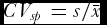 $CV_{sp} = s/\bar x$
.
$CV_{sp} = s/\bar x$
.
ANOVA was performed with the M-STAT statistical package (MSTAT-C, version 1.41, Crop and Soil Sciences Department, Michigan State University, USA) to measure the heterogeneity among PLs, where CV was computed by the formula $CV_{pl} = \sqrt {EMS} /\bar x$
, with EMS corresponding to the mean square error.
$CV_{pl} = \sqrt {EMS} /\bar x$
, with EMS corresponding to the mean square error.
RESULTS
The maize hybrid ‘B73xMo17’
Data quoted in Table 1 show that as regards yield per plant the overall mean was 449 g, with a CVsp of 38%. As expected, heterogeneity was greater along the longer side of the breadthwise direction. Indicatively, the TBG of grain yield of seven PLs was higher when allocated breadthwise rather than lengthwise, that is, 17 vs. 8.1%.
Spatial heterogeneity is further depicted in the uniformity map of Figure 1 where the yield range of 28 equal PLs (337–526 g) reflected a TBG relevant to the overall mean of 42%. The respective CVsp range was 30 to 42%. Twelve MSD out of the 28 PL yield means reflected significant residuals (Table 1). The NN analysis for 28 simulated entries reduced the TBG to 19% (lengthwise analysis) and 22% (breadthwise analysis), and the respective MSD values to 5 and 8. In terms of the plant height, mean values varied from 178 up to 212 cm (TBG of 17%), and 16 out of the 28 means differed significantly from the overall mean of 199 cm. The NN method resulted in TBG of 4.7 and 6.1% (MSD of 2 and 4). The ear height of the 28 PLs ranged from 83.1 up to 104 cm (TBG of 22%) with 16 of them significantly differing from the overall mean (95 cm), and the NN analysis gave TBG of 6.2 and 9.7% (MSD of 2 and 3). The average ear length of 235 mm differed significantly in 12 out of the 28 PL means of 225 to 243 mm, corresponding to TBG of 7.7%, and the NN analysis reduced TBG to 3.0 and 6.1% (MSD of 2 and 5).
In the case of 16 simulated entries, grain yield means corresponded to 38% TBG and included five significant residuals (MSDs). Comparatively, the RCBw exhibited a similar TBG including double MSDs, while the RCBb declined TBG to 6.8% without any significant residual. The NN method decreased the TBG to 17% for the lengthwise and 14% for the breadthwise arrangement; however, the MSD increased to seven for the former and decreased to one for the latter. Concerning plant height, the best RCBb reduced TBG to 4.2% and the MSD to 8, and the worst RCBw did not make any correction. The NN alternative gave TBG values of 4.6 and 9.4%, and MSD of 4 and 7. With regard to ear height and ear length, and compared with the PL configuration, the RCBb reduced the TBG nine-fold and six-fold, respectively, zeroing the MSD in both. Instead, the RCBw arrangement retained the level of TBG and increased the MSD from 10 to 11 for ear height and from 7 to 10 for ear length. The NN analysis, gave 6 and 4 MSD for lengthwise and breadthwise arrangement in the matter of ear height. The respective values in relation to ear length were 10 and 5.
As regards grain yield of seven simulated entries, the RCB7w resulted in almost double heterogeneity compared with the adverse breadthwise allocation (31 vs. 17% TBG and 5 vs. 4 MSD). Instead, the RCB7b reduced the TBG to 3.1% and zeroed the MSD. ANOVA resulted in CVpl of 5.4% for the RCB7w and 13.5% for the RCB7b. When the ANOVA was performed for several randomized scenarios of the RCB7, a negative connection between TBG and CVpl was found (Figure 2). The NN analysis resulted in less heterogeneity than the common PL arrangement, that is, 6.4 vs. 8.1% TBG (one MSD for both) for the desirable lengthwise orientation, but retained almost the same heterogeneity (16 vs. 17% TBG and four MSD for both) for the breadthwise orientation. The outcome of the LD7 analysis was 17% TBG and 4 MSDs. As regards plant height and ear height, for the best RCB arrangement there was still one MSD (vs. three and six of the lengthwise PL arrangement). Against PL7, the NN analysis gave the same (plant height) or less (ear height and length) MSD values for both directions. The LD7 substantially lowered the TBG, however, five, three and two MSDs were computed for plant height, ear height and ear length, respectively.
The relationship between the level of the top-to-bottom gap (TBG) with the coefficient of variation among plots (CVpl) within blocks which resulted when ANOVA was performed for the RCB7 of Figure 1 for different randomizations.

The NN32 analysis did not change the 46% TBG of 32 PLs (Figure 3). Since resolving the major direction of the spatial heterogeneity blocking the lengthwise direction would be desirable, for comparison purposes, the 32 PL assumed to represent four blocks of eight entries were analysed in both directions (see the Table below Figure 1). In the longitudinal arrangement prudent randomization (RCB8ln/b) resulted in a mean range of 444 to 454 g (TBG of 2.7%) and zero MSD, whereas the most adverse randomization (RCB8ln/w) gave a mean range of 389 to 518 g (TBG of 28%) and 6 out of the 8 MSD (not shown). The CVpl value resulting from ANOVA was higher for the former (12%) than the latter (4.7%). The breadthwise randomization resulted in a mean range of 431 to 462 g (TBG of 6.9%) and zero MSD for the RCB8br/b, and 380 to 516 g (TBG of 30%) and six MSD for the RCB8br/w. The CVpl values from ANOVA were 12.4 and 6.2%, respectively.
The entry residual from the grand mean as an index of the alleviation level of spatial heterogeneity obtained by the nearest-neighbour (NN) and the honeycomb design (HD) methods versus the plot (PL) arrangement in two grain yield trials. Each model is followed by the number of simulated entries and the top-to-bottom gap of entry means is given within parentheses, i.e., PL-16(51%) implies that means of 16 entries allocated in random plots exhibited 51% TBG relevant to the grand mean. Trial areas (m2) and statistics of single plants are shown, i.e., grand mean (
$\bar x$
), coefficient of variation (CVsp) and the number of plants measured (n). Solid points along a line correspond to means significantly differing from the grand mean.

As far as the honeycomb entry arrangement is concerned, the mean ranges of the potential designs simulating 3–37 entries are given in Table 2, and the respective TBGs and the number of means differing significantly from the overall mean are shown in Table 3. In general, increasing the number of entries resulted in wider variation among their means and a greater incidence of deviating means. Indicatively for grain yield, the lowest TBG (3.0%) was observed in an HD4 model and the highest one (24% with two MSD) in an HD31 analysis. A positive correlation was measured between the number of entries and the respective average TBG (Figure 4). For the seven designs that belong to the grouped set (corresponding to 4, 9, 12, 16, 25, 27 and 28 entries) different constant (k) values did not affect the outcome resulting in absolute the same mean ranges (Table 2). For the ungrouped designs, different k constants gave different mean ranges, but over all did not play any crucial role in experimental precision, and the same applied to trial orientation. For example, in the HD21 and HD37 designs for which two k values exist, the higher k resulted in more MSD in the breadthwise orientation and the lower k resulted in more MSD in the lengthwise orientation. For the HD31 design, the opposite was true. In terms of experimental orientation, out of the total 80 mean ranges for each orientation (Table 2), at least one significant residual was included in 21 for the breadthwise and 26 for the lengthwise orientation (Table 3).
The relationship between the number of simulated entries included in a honeycomb design, and the degree of the respective average top-to-bottom mean value gap as a percentage of the trial mean, in relation to yield per plant of maize hybrid ‘B73xMo17’ and wheat cultivar ‘Nestos’. The slopes of the linear correlations (significant at p < 0.001) indicate three-fold higher rate of TBG increase in the wheat compared to the maize trial.

For yield, the TBG of 4% of the HD7 analysis (k = 2) across the entire experimental area (Table 3) inflated to 8.9, 11 and 13% when applied to the left, middle and right third, respectively (Figure 1); none showed significant deviation, however. The HD7 (Table 3) averaged higher TBG (4.9%) compared with the RCB7b (Table 1); however, no significant residual resulted. The HD7 model gave better results compared with the NN analysis of both directions. For plant height, the HD7 gave TBG values of 0.9 to 1.3% (no MSD), whereas the respective values for the RCBb, RCB7w, NN7ln and NN7br were 2.1% (1), 11% (3), 5.4% (3) and 7.2% (5). For ear height, the HD7 gave TBG values of 1.2 to 2.0% (no MSD), whereas the respective values for the RCBb, RCB7w, NN7ln and NN7br were 2.3% (1), 13% (6), 6.7% (3) and 6.2% (4). For ear length, the HD7 gave TBG values of 0.6 to 1.1% (no MSD), whereas the respective values for the RCBb, RCB7w, NN7ln and NN7br were 0.8% (0), 4.5% (5), 1.8% (3) and 2.9% (4).
In terms of 16 entries, for yield the HD16 exhibited less precision than the RCB16b resulting in TBG of 10% (no MSD) in the breadthwise analysis and 11% (one MSD) in the lengthwise analysis. Nevertheless, the HD16 model was more precise than the NN analysis. For plant height, the HD16 was more effective (TBG of 0.9% with no MSD) than the RCB and NN analysis. Regarding ear height, the HD16 matched the effectiveness of RCB16b, exhibiting TBG of 0.7 to 0.8% (no MSD). Regarding ear length, the HD16 gave TBG of 0.9% (no MSD) for breadthwise direction matching the RCB16b. For the lengthwise direction, TBG was 1.0% (one MSD), whereas the NN16ln gave 3.1% TBG and the NN16br 3.0% TBG, with 10 and 5 MSD, respectively.
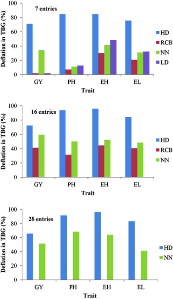
In the case of four simulated entries and for grain yield in particular, the honeycomb analysis averaged TBG of 4.1% with one significant residual, and the RCB4b and RCB4w resulted in TBG of 6.9 and 19%, respectively; in both, two out of the four means differed significantly from the overall mean (not shown). The 14% TBG of the LD4 was accompanied by three MSDs for yield. The LD4 configuration resulted in 4.8% TBG and 4 MSD concerning plant height, 4.3% TBG and 3 MSD for ear height, and 1.5% TBG and 3 MSD for ear length. For comparison purposes, data from Tables 1 and 3 were summarized in Figure 5 demonstrating the average deflation in TBG obtained by HD and the classical procedures, concerning 7, 16 and 28 entries. The HD model averaged the highest deflation, i.e., of 70, 90, 92 and 81% for grain yield, plant height, ear height and ear length, respectively. The respective achievements were 22, 19, 37 and 31% for RCB, 48, 43, 52 and 40% for NN and 2, 13, 48 and 32% for LD.
Comparison of the honeycomb model (HD) for 7, 16 and 28 entries with the respective randomized complete block (RCB) of four replicates, the nearest-neighbour (NN) model and the lattice design (LD), concerning the deflation in spatial heterogeneity for grain yield (GY), plant height (PH), ear height (EH) and ear length (EL), as percentage reduction in TBG relevant to TBG measured in the plot (PL) configuration (the breadthwise direction for seven entries). Pooled data obtained from Table 3 (HD) and Table 1 (RCB, NN and LD).
The wheat cultivar ‘Nestos’
Spatial heterogeneity of the wheat experiment (Figure 6) was expressed by 56% CVsp; divided into 16 PLs gave a mean range of 23.3 to 39.0 g, corresponding to a 51% TBG and including 9 MSDs (Figure 3). The NN and HD remedy techniques for the same number of PLs gave TBG of 38 and 22%, respectively, with three MSDs for the former and none for the latter. In the case of the honeycomb models, significant residuals were computed for the HD19 of k = 11 (one MSD), the HD21 of k = 4 (one MSD) and the HD25 (two MSDs), and the correlation of TBG with the number of entries was significant (Figure 4). When four entries were under consideration, the HD4 and RCB4b succeeded in zeroing MSD (TBG of 6.1 and 3.0%, respectively) while the four means of the LD4 significantly deviated (TBG of 10%) (not shown).
Smoothed variability map constructed on the single-plant grain yield (g) from the uniformity trial of the wheat cultivar ‘Nestos’. The coloured legend on the right gives the yield range of small plot units corresponding to the respective delineated area. An illustration of the possible honeycomb arrangement of seven entries demonstrates that every entry (e.g., entry 7) is evenly positioned across the entire experimental area on an equilateral triangle pattern, so the spatial heterogeneity can be sampled and overcome in the most effective way when comparing different entries. The circles demonstrate that the performance of each plant (positioned in the centre) can be expressed in relation to the mean of the plants within a circle of chosen size, constituting thus a moving fixed complete replicate, distributed to all directions. The moving fixed complete replicate allows the nearest-neighbour approach to be easily established, e.g., yield of the plant coded 7 or 1 is adjustable to the average performance of 7 (interior circle) or 19 (exterior circle) or more entries/plants, ensuring the most objective single-plant selection within a particular entry. (Based on Fasoulas and Fasoula, Reference Fasoulas and Fasoula1995).

DISCUSSION
The general impacts
Spatial heterogeneity is a ubiquitous feature in natural ecosystems (García–Palacios et al., Reference García–Palacios, Maestre, Bardgett and de Kroon2012; Li et al., Reference Li, Li, Ma, Fan and Wang2010). In plant breeding, yield is always one of the main objectives affected by numerous factors comprising spatial heterogeneity (Ball et al., Reference Ball, Mulla and Konzak1993; Brownie et al., Reference Brownie, Bowman and Burton1993; Stroup et al., Reference Stroup, Baenziger and Mulitze1994; Vollmann et al., Reference Vollmann, Winkler, Fritz, Grausgruber and Ruckenbauer2000). Spatial heterogeneity was comparatively lower in maize rather than wheat (Figures 3, 4). This classification was reflected by the significant residuals of simulated entries and/or the overall CVsp values. It was the outcome of both genotype vulnerability to environmental forces and the conditions under which each trial was conducted. The wheat cultivar had been qualified as a genotype that lacks genetic buffering and is thus prone to acquired variance (Tokatlidis et al., Reference Tokatlidis, Xynias, Tsialtas and Papadopoulos2006). Trial of the maize hybrid was three-fold larger but exhibited lower spatial variation attributable to genotype stability or a less fluctuating environment or both.
The results suggest that spatial heterogeneity in maize field trials may simultaneously influence not only grain yield but other agronomic characteristics as well, in agreement with Vollmann et al. (Reference Vollmann, Winkler, Fritz, Grausgruber and Ruckenbauer2000) concerning soybean trials. Variations in soil parameters have been reported to affect element concentrations in grain, grain yield and protein content of wheat in a correlated manner (Berndtsson and Bahri, Reference Berndtsson and Bahri1995; Mulla et al., Reference Mulla, Bhatti, Hammnond and Benson1992). Inability to combat spatial variation could cause biased estimates of heritability (Helms et al., Reference Helms, Orf and Scott1995; Magnussen, Reference Magnussen1993; Rosielle, Reference Rosielle1980), decreased response to selection and reduced precision of testing statistics (Vollmann et al., Reference Vollmann, Winkler, Fritz, Grausgruber and Ruckenbauer2000). Procedures that correct for the effects of spatial variability can require elaborate statistical designs (e.g., lattice or NN designs); however, they are rarely used by breeders, who prefer classical field-PL designs, thus maintaining lower efficiency (Ball et al., Reference Ball, Mulla and Konzak1993; Rosielle, Reference Rosielle1980), particularly for characteristics other than yield (Vollmann et al., Reference Vollmann, Winkler, Fritz, Grausgruber and Ruckenbauer2000).
Effectiveness of the honeycomb model
The first and inviolable rule of the honeycomb breeding method is absence of competition. The reasons have been thorougly explained previously (Fasoula and Fasoula, Reference Fasoula and Fasoula2000; Fasoula and Tokatlidis, Reference Fasoula and Tokatlidis2012; Fasoulas, Reference Fasoulas1993; Fasoulas and Fasoula, Reference Fasoulas and Fasoula1995; Kyriakou and Fasoulas, Reference Kyriakou and Fasoulas1985; Tokatlidis et al., Reference Tokatlidis, Has, Mylonas, Has, Evgenidis, Melidis, Copandean and Ninou2010) and are beyond the scope of this paper. This work focuses on the potential effectivenenes of honeycomb experimental designs, and draws interesting comparisons with RCB, NN and LD.
Analysis of the maize hybrid data shows that there is no need for concern about orientation in field experimentation according to the honeycomb pattern. Despite the differential distribution of spatial variation (Figure 1), none of the directions was found to be advantageous and their differences were relatively low (Tables 2, 3). The same applies to the k constants. As regards the grouped HDs, different k resulted in absolutely the same outcome, whereas for the ungrouped ones, the differences were relatively low. The systematic entry arrangement of the honeycomb layout regardless of the number of entries and the k constant chosen to construct the design (Fasoulas and Fasoula, Reference Fasoulas and Fasoula1995) offers a uniform entry distribution to all directions. The longitudinal arrangement gave mostly better results in NN statistical analysis (Table 1). The same applies to the RCB8 because of the within-blocks higher heterogeneity for the breadthwise direction (lower TBGs and CVpl values for RCB8ln than RCB8br). Heterogeneity among PLs within a block causes the estimated difference between two treatments to vary across blocks; the greater the heterogeneity within blocks, the greater the variation in estimates of treatment effect and the lower the precision of the study (Brownie et al., Reference Brownie, Bowman and Burton1993; Gusmao, Reference Gusmao1986; Stroup et al., Reference Stroup, Baenziger and Mulitze1994; Vollmann et al., Reference Vollmann, Buerstmayr and Ruckenbauer1996, Reference Vollmann, Winkler, Fritz, Grausgruber and Ruckenbauer2000).
Another important inference is that for up to nine entries, statistically the HDs succeeded in almost absolute sampling the spatial heterogeneity (Table 3). The RCBs did the same regarding the presupposition of favourable randomization, i.e., the RCB7b and RCB16b (Table 1) as well as the RCB8b zeroed the MSD while the RCB4b gave two MSDs. Nevertheless, the respective adverse randomizations not only exhibited absolute failure to remedy the spatial heterogeneity, but even deteriorated it (e.g., the RCB7w in Table 1). Hence, taking into account the very low possibility of prudent randomization, the HD appears advantageous. For example, in the case of seven entries replicated four times the possibility of a particular randomization is one per 50404, implying that RCB7b (and RCB7w) is unrealistic. Considering the magnitude of 31% TBG of the RCB7w, the most probable level of 15 to 20% TBG (reflecting just 2% deflation and absolute failure as Figure 5 demonstrates) is far from sufficient (i.e., the 16% of the NN7br included three out of seven significant residuals) (Table 1). On the other hand, the NN model produced inadequate deflation of differences, and sometimes failed completely (Table 1, Figure 3). Indeed, the literature presents contrasting accounts of NN analysis. Pro the NN analysis were the results of Townley-Smith and Hurd (Reference Townley-Smith and Hurd1973), and Vollmann et al. (Reference Vollmann, Buerstmayr and Ruckenbauer1996) indicated it was more efficient than both the RCB and LDs. Scharf and Alley (Reference Scharf and Alley1993) and Stroup et al. (Reference Stroup, Baenziger and Mulitze1994) recommended it to improve accuracy and precision compared with RCB analysis. However, Zimmerman and Herville (Reference Zimmerman and Harville1991) found random field methods to be more accurate than NN procedures, and Helms et al. (Reference Helms, Orf and Scott1995) did not find any advantage of NN over unadjusted selection criteria in two soybean populations. Rosielle (Reference Rosielle1980) found an LD more efficient for control of intra-site error compared with both NN and RCB designs, and Vollmann et al. (Reference Vollmann, Winkler, Fritz, Grausgruber and Ruckenbauer2000) found both lattice analysis and the NN method to be far more efficient than randomized block analysis in modelling spatial variations.
Using a special analysis technique can improve precision, but selecting the most appropriate analysis for a given set can be hard (Brownie et al., Reference Brownie, Bowman and Burton1993). Spatial homogeneity within blocks is extremely uncommon and the efficiency of the RCB design tends to be poor in trials involving a large number of treatments (Brownie et al., Reference Brownie, Bowman and Burton1993; Stroup et al., Reference Stroup, Baenziger and Mulitze1994). Breeders qualify their trials on the CVsp of ANOVA and often discard trials with CVsp > 15% as unacceptable (Stroup et al., Reference Stroup, Baenziger and Mulitze1994). However, if this is the case, the negative relationship between the CVsp values obtained by ANOVA with the respective TBGs (Figure 2) is interesting, implying contrasting inferences for two desirable outcomes. Replication is in itself an attempt to account for the existence of soil's spatial variability. However, it is a crude technique given the complex patterns of spatial variability that exist, and there is no way to lay out blocks that will successfully account for spatial yield variability (Scharf and Alley, Reference Scharf and Alley1993). To increase precision in such a trial, one approach is to reduce block size by employing an incomplete block design such as LD designs (Brownie et al., Reference Brownie, Bowman and Burton1993). LDs, however, have certain disadvantages over RCBs in terms of the number of treatments and the field layout (Rosielle, Reference Rosielle1980). Concerning the NN method, Ball et al. (Reference Ball, Mulla and Konzak1993) recommended it as a means to remove the effects of spatial dependence on PL yield deviations from the treatment mean. Brownie et al. (Reference Brownie, Bowman and Burton1993) recommended that NN analysis should ignore blocks to avoid artificial discontinuities, whereas uniterated analysis lacks efficiency and iterated produces inflated Type I error rates. The HDs compromise the main principles of the above statistical schemes, i.e., blocking, replication, systematic distribution to all directions, plus potential NN adjustment on the same baseline. These features can be seen in Figure 6, corresponding to seven entries. A complete block should involve the seven entries, as in the case of the interior circle. The fixed block is repeatable many times throughout the trial, and its shape ensures the greatest within-block homogeneity. Every entry is evenly distributed across the area on an equilateral triangular pattern sampling the spatial heterogeneity. Every plant/entry that occupies the centre of a circle can be qualified on the average performance of the plants included within the circle, i.e., the moving circular average (Fasoulas, Reference Fasoulas1987), matching the moving average method of Knott (Reference Knott1972). The systematic entry arrangement ensures that the same entries are always included in the circle, so the technique simulates that of the check PL of Briggs and Shebeski (Reference Briggs and Shebeski1968), despite the ‘paucity’ of a common control. In fact, the technique of the honeycomb moving circular average was performed in both trials using a circle size of 60 plants. Nevertheless, the results were essentially similar to the presented unadjusted means and thus of no consequence from the perspective of this paper.
Difficulties of dealing with spatial variation are pronounced with a high number of entries. In the RCB model, in experiments with more than 8 to 12 PLs per block, the layout becomes problematic because the assumption of spatial homogeneity within blocks is extremely uncommon (Stroup et al., Reference Stroup, Baenziger and Mulitze1994). Absolute failure resulted in maize from the NN32 (Figure 3). Increasing the level of entries reduced ability of the HD model to cope with the spatial variation, and slopes of the linear correlations indicated almost three-fold higher rate of TBG increase in the wheat trial compared to the maize one (Figure 4). Obviously, to encounter huge spatial heterogeneity, the number of entries is a key factor. Larger area of the moving circular complete block in a higher number of entries reasonably inflates the mean differences because of greater intra-block variation. For instance, the exterior circles in Figure 6 correspond to the moving circular complete block of the HD19 design, which is apparently more heterogeneous than the interior of the HD7. Fasoulas (Reference Fasoulas1987) maintained arguably that adjustment of the size of the moving block is expected to be effective between certain limits only, i.e., large blocks are preferably used when the number of entries is large, while the opposite is true for low entry selection pressures. The size of the moving circular complete block is also determined by the inter-plant distance. Therefore, concerning honeycomb breeding choice of an optimal rather than huge inter-plant distance to meet the condition of absence of competition appears very important. The issue is a matter of both crop and genotypes under evaluation, as Tokatlidis et al. (Reference Tokatlidis, Has, Mylonas, Has, Evgenidis, Melidis, Copandean and Ninou2010) evidenced in maize. The number of entries is determined by the genotype and treatment, and limiting them is not always realistic. Considering the results of HD7 analysis for yield in the trial shown in Figure 1 for the entire area and for the three parts, it looks as though the number of replicates is crucial. For the partial analysis, the entry sample size is more than 100 plants per entry and is statistically adequate, and the outcome is deemed successful. However, over the entire experiment, the same analysis succeded in substantially greater deflation of the means’ deviation from the grand mean (TBG of 4 vs. up to 13%) despite the three times larger area. This is a very important inference, implying that when many entries are included in the honeycomb procedure increasing the replicates per entry will improve effectivenes in correcting spatial variation despite the concomitant greater overall spatial heterogeneity. According to Fasoula (Reference Fasoula2013), the honeycomb model was invented for evaluation and selection to cover two needs. The first is the removal of the masking effects of soil heterogeneity, and the other to exploit the advantages offered by soil heterogeneity to select for stability.
Due to lack of previous relevant research, one could hypothesize that inferences drawn are data specific (specific crops, traits and fields), hence, further research is imperative. The HD may have not yet gained popularity among breeders. In classical models, the PL as experimental unit is preferred to simulate true growing conditions. However, in case of the mono-genotypic cultivar (i.e., inbred line and/or single-cross hybrid) growing condition represents an absolute pure stand. Therefore, during the breeding process seeking for the outhstanding genotype actual farming condition is not feasible since the classical PL would comprise a mixture of genotypes. Further, competition may exert obstructive influence on genotypes potential of excellent performance in pure stand (Fasoula and Fasoula, Reference Fasoula and Fasoula2000; Tokatlidis, Reference Tokatlidis2015). Rather, the honeycomb model assuming the individual plant as experimental unit enables experimentation at nil-competition to erase the barrier of competition. This combined with the effectiveness of sampling the spatial heterogeneity renders the model of long perspective of promoting progress through selection as the so far relevant research indicated in several crops, even within too narrow gene pools (Tokatlidis, Reference Tokatlidis2015) unexploitable through the PL model. Further research on the required distance to grow individual plants independent of competition which vary among crops (depending mainly on the crop ‘size’), and invention of appropriate hardware and software may promote wider adoption of the honecycomb breeding among breeders.
CONCLUSION
Despite the increased spatial heteogeneity induced by the large experimental surface owed to high inter-plant distances, the overall inference drawn from the current study is that the honeycomb experimental design samples spatial heterogeneity. It comprises the main elements met in other models, i.e., blocking, replication, NN pattern adjustment on the same baseline, plus distribution to all directions with systematic rather than randomized configuration; thus, it appears advantageous over the classical experimental designs like the RCB, the NN method and the lattice pattern. Additionally, breeders do not need to be concerned with the pattern and orientation of soil variability in order to decide on the layout of the field plan, the shape, size and orientation of the PLs and grouping of the PLs into blocks. To optimize sampling of spatial heterogeneity via the honeycomb pattern, optimal inter-plant distance ensuring exclusion of plant-to-plant interference for resources and the number of replicates per entry are of paramount importance. The former is a matter of the crop, while more replicates is mandate with increased size of the moving circular complete block (e.g., larger inter-plant distance or number of entries). They are challenging issues both deserving further investigation.
Acknowledgement
Author is grateful to his anonymous reviewers for their critical review, and constructive comments and suggestions, contributing to the paper's essential improvement.



