2 Models of Portfolio Allocation: The Unsuitability of Current Approaches

Most studies of quantitative portfolio allocation—the question of “how many” portfolios parties receive—share several features: (1) government parties are the units of analysis; (2) the dependent variable is defined as party portfolio share; (3) one of the covariates is a party’s legislative size relative to its partners; and (4) the analysis entails a simple linear regression of portfolio share on seat share, sometimes with additional covariates like bargaining power, proposer status, or interactions between seat share and contextual features of the bargaining environment. Unfortunately, this empirical strategy overlooks the unique structure of portfolio allocation data and is ill-suited to its analysis.

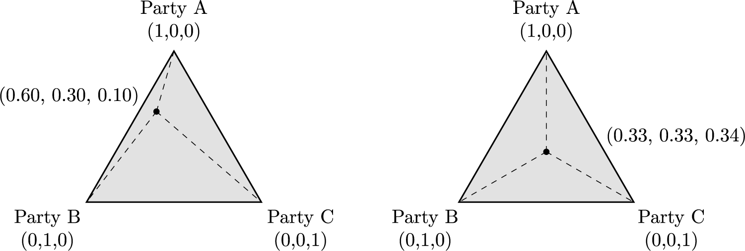
Both portfolio and seat share are inherently compositional: they are proportions representing “parts of a whole” and must sum to one across all parties in a given government. With few exceptions (discussed below), this fundamental property is largely ignored in the literature. Most scholars employ least-squares regression (OLS), which assumes that observations are independent, the dependent variable is unbounded, and the relationship between predictors and the outcome is linear. None of these assumptions hold in the compositional setting. As parts of a whole, individual observations are necessarily interdependent: if one party’s portfolio share increases, at least one other party’s must decrease. In addition, portfolio shares are bounded between 0 and 1, which means that their potential to change is constrained near the limits of the scale, undermining the assumption of linear marginal effects. Collectively, these features imply that portfolio and seat shares lie not in unconstrained Euclidean space but in a unit simplex (Aitchison Reference Aitchison1982, Reference Aitchison1986).Footnote ¹ Figure 1 illustrates this geometry in the three-party case, where shares are expressed as barycentric coordinates: the right panel shows a roughly even division, while the left panel depicts a distribution closer to the simplex bounds.

Figure 1 Unit simplex diagrams with different portfolio (seat) shares.

2.2 The ALR+SUR Solution

Political scientists have long recognized the limitations of applying OLS to compositional data. In early studies of alternative approaches (e.g., Honaker et al. Reference Honaker, Katz and King2002; Jackson Reference Jackson2002; Katz and King Reference Katz and King1999; Tomz et al. Reference Tomz, Tucker and Wittenberg2002), the outcome of interest was typically each party’s share of the vote across electoral districts. More recent work has applied compositional methods to domains such as public budgeting (e.g., Clayton and Zetterberg Reference Clayton and Zetterberg2018; Philips, Rutherford, and Whitten Reference Philips, Rutherford and Whitten2016), where the dependent variable represents the allocation of a fixed resource (e.g., spending shares across categories).

To accommodate the boundedness and constant-sum constraint inherent in such data, these studies employ the ALR transformation introduced by Aitchison (Reference Aitchison1982, Reference Aitchison1986). The ALR maps a K-part composition from the unit simplex S ^K−1 ⊂ ℝ ^K to ℝ ^K−1 by expressing each component relative to a designated reference part. For example, choosing component v _n as the reference yields the transformed vector:

$$\begin{align*}\left[ \ln\left( \frac{v_1}{v_n} \right), \ln\left( \frac{v_2}{v_n} \right), \dots, \ln\left( \frac{v_{n-1}}{v_n} \right) \right]. \end{align*}$$

This transformation preserves the relative information in the composition while allowing analysts to apply linear modeling techniques in an unconstrained space.Footnote ³

However, because all log-ratios share a common denominator, the ALR transformation induces strong correlations among the transformed components. This violates the assumption of independent errors across equations and, if unaccounted for, leads to inefficient estimates and invalid standard errors. To address this, nearly all political science applications of ALR have coupled it with SUR, which models the log-ratio equations jointly while accounting for contemporaneous correlation in the residuals. SUR estimation is particularly well-suited to this task: when the covariates differ across equations, it improves efficiency; when the covariates are the same, it still yields more accurate standard errors (Zellner Reference Zellner1962). Without SUR—or some alternative method to account for residual dependence—the use of ALR alone is inadequate. It fails to respect the interdependence of compositional parts and will generally produce misleading inferences.

One might think that the ALR+SUR strategy could easily be extended to portfolio allocation. Yet as Indridason (Reference Indridason2015) notes, the approach encounters fundamental limitations in this context. Most obviously, SUR requires a fixed system of equations across all observations. But in the context of portfolio allocation, the number of government parties—and hence the number of compositional components—varies across governments. When the number of parties changes, the number of ALR-transformed variables changes accordingly, making it impossible to specify a consistent system of equations for joint estimation. This structural mismatch renders SUR inapplicable, and therefore makes ALR+SUR effectively unusable.

Even apart from this fundamental barrier, the ALR transformation itself becomes problematic when applied to varying coalition structures. Because it is defined relative to a single baseline component, ALR assumes that the same party occupies the denominator role in every observation. In within-country studies of electoral competition, at least where there exists one party that competes in every district, this assumption is satisfied; researchers can use that party (e.g., the UK Conservative Party) as a constant reference component.

But in portfolio allocation, the identity of governing parties varies both across countries and over time. As a result, no stable reference party exists. This presents a serious complication: when the reference party varies across governments, each log-ratio is anchored to a different baseline. This introduces observation-specific scaling: systematic differences in the chosen baseline are pushed into the error term or confounded with covariates, yielding biased coefficients and misleading inference. In short, ALR+SUR relies on two structural conditions—invariant baselines (ALR) and fixed dimensionality (SUR)—that do not hold in this setting. Analysts must therefore turn to an alternative that remains valid when the number and identity of components vary.

3 The ILR Transformation

The limitations of the ALR+SUR framework might suggest that log-ratio transformations are poorly suited for analyzing portfolio allocation.Footnote ⁴ However, this impression is misleading. ALR is just one member of a broader family of log-ratio transformations developed to handle the unique constraints of compositional data. Critically, one alternative—the ILR transformation introduced by Egozcue et al. (Reference Egozcue, Pawlowsky-Glahn, Mateu-Figueras and Barceló-Vidal2003)—avoids the central pitfalls of ALR+SUR. It does not require a fixed reference component, can be applied to compositions of varying dimensionality, and produces transformed variables that are uncorrelated and geometrically well-behaved.

Like the ALR, the ILR transformation maps compositions from the constrained unit simplex $S^{K-1}$ into $\mathbb {R}^{K-1}$ , thereby allowing standard regression techniques to be applied. But unlike ALR, which expresses each part relative to a single denominator, ILR constructs $K-1$ orthogonal coordinates—called balances—based on a sequential binary partition (SBP) of the K compositional parts. Each ILR coordinate compares the geometric mean of one subset of parts to the geometric mean of its complement:

$$\begin{align*}\text{ILR}_b = \ln\left( \frac{g(S_b)}{g(T_b)} \right), \end{align*}$$

where $g(S_b)$ and $g(T_b)$ denote the geometric means of disjoint subsets such that $S_b \cup T_b = \{1, \dots , K\}$ and $S_b \cap T_b = \emptyset $ . Typically, $S_b$ contains a single part and $T_b$ the remaining $K-b$ parts.

For example, in a five-party government with parties A through E, one valid SBP produces:

$$\begin{align*}\text{ILR}_1 = \ln\left( \frac{A}{\sqrt[4]{B \cdot C \cdot D \cdot E}} \right), \quad \text{ILR}_2 = \ln\left( \frac{B}{\sqrt[3]{C \cdot D \cdot E}} \right), \end{align*}$$

$$\begin{align*}\text{ILR}_3 = \ln\left( \frac{C}{\sqrt{D \cdot E}} \right), \quad \text{ILR}_4 = \ln\left( \frac{D}{E} \right). \end{align*}$$

Each balance contrasts one party with the geometric mean of a successively smaller group of others. The ordering of parts is arbitrary, but any valid SBP produces an orthogonal basis in the simplex (Egozcue et al. Reference Egozcue, Pawlowsky-Glahn, Mateu-Figueras and Barceló-Vidal2003, 290–292), ensuring that each balance captures unique, uncorrelated information.Footnote ⁵

As with ALR, analysts must specify a basis when constructing ILR coordinates. In ALR, this means choosing a reference category; in ILR, defining the SBP. These choices affect the labeling and interpretation of coefficients but not the underlying results: model fit and predictions are invariant to either choice. In ALR, coefficients from one baseline can be obtained from another through simple subtraction; in ILR, the same principle applies, though implemented through orthogonal transformations.Footnote ⁶ While orthogonal rotation is more cumbersome than ALR’s subtraction, it does not change the mathematics of the model. Thus, in both approaches, baseline or partition choices matter only for interpretation, not inference.

Most crucially for portfolio allocation, the ILR transformation solves the dimensionality problem. Unlike ALR+SUR—which requires the same set of components and a fixed denominator across observations—ILR constructs $K_g\!-\!1$ balances from the parts actually present in each government g. If one government includes five parties and another only three, ILR simply constructs four balances for the former and two for the latter. As party systems change across cabinets, ILR thus permits pooling without imputation, collapsing parties, or estimating separate models by composition. By contrast, earlier strategies—e.g., imputing shares for non-competing parties, fitting distinct ALR+SUR systems for each pattern of party absence, or collapsing minor parties into “Other” (Honaker et al. Reference Honaker, Katz and King2002; Jackson Reference Jackson2002; Katz and King Reference Katz and King1999; Tomz et al. Reference Tomz, Tucker and Wittenberg2002)—impose strong assumptions, fragment analyses, and undermine comparability. In short, ILR provides a single coherent framework that accommodates variation in both the number and identity of parties while preserving the simplex constraints and the joint nature of the composition.Footnote ⁷

4 Monte Carlo Simulations

We evaluate the ILR approach via Monte Carlo simulations, benchmarking it against standard OLS estimators. Because our later empirical application uses multilevel models, we include both single- and multilevel specifications for the simulations. ILR is estimated only in multilevel form and compared to four OLS alternatives: OLS–LOO, OLS–LOO–CSE, and their multilevel counterparts OLS–ML and OLS–ML–CSE. All OLS variants use the “leave-one-out” (LOO) strategy; CSE models cluster-robust standard errors at the government level. We focus on two parameters: the mean slope linking seats to portfolios ( $\bar {\beta }$ ) and the random-slope variance ( $\tau $ ).

4.1 Design

In each replication, we simulate seat shares for the parties in each government as valid compositions on the simplex, and generate portfolio shares from:

$$\begin{align*}z_{jg} \;=\; \beta_g \, s_{jg} + \varepsilon_{jg}, \qquad \beta_g \sim N(\bar{\beta}, \tau^2), \qquad \varepsilon_{jg} \sim N(0,\sigma^2), \end{align*}$$

where $s_{jg}$ and $z_{jg}$ are ILR coordinates of seats and portfolios. The overall intercept is fixed at zero. We treat governments as consisting of different parties across cases, which reflects the empirical reality of cabinet formation and immediately rules out ALR, which requires the same reference denominator across all observations.

We fix the number of parties at $K=3$ , the median cabinet size in our data, and set the other parameters as follows:

1. (1) A mean slope in ILR space of $\bar {\beta }=0.70$ . On the original simplex, this corresponds approximately to 4:3 proportionality between portfolios and seats, or an effective slope of about 0.74.Footnote ⁸ All hypothesis tests reported below are conducted in simplex space, treating 0.74 as the true value.

2. (2) A random slope SD of $\tau =0.13$ , defined in ILR space, with the random intercept fixed at zero.

3. (3) A residual SD of $\sigma =0.36$ .

We evaluate estimator performance across ten bins of a variable we call the boundary proximity index (BPI), which is defined at the government level as,

$$\begin{align*}BPI_g = \frac{\sum_{j=1}^{K} p_{jg}^2 - \tfrac{1}{K}}{1 - \tfrac{1}{K}} \,, \end{align*}$$

where $p_{jg}$ is party j’s portfolio share in government g. Values near zero indicate balanced allocations at the simplex center, while values near one reflect concentration near the boundary. We use this index because treating compositional outcomes as unconstrained is most problematic at high BPI, where OLS estimators should perform worse. Each BPI bin contains 500 replications of 300 simulated three-party governments (i.e., 150,000 per bin). Bins go from low to high concentration: lower bins collect governments near the simplex center, higher bins those near the boundary.

4.3 Results for $\hat {\beta }$

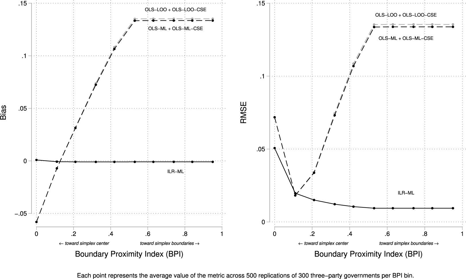
Figures 2 and 3 summarize the findings for $\hat {\beta }$ when $K=3$ .Footnote ¹⁰ Figure 2 shows that ILR–ML accurately recovers the true slope across the BPI range: bias remains near zero and RMSE is minimal. By contrast, OLS variants underestimate when $BPI < 0.10$ and overestimate once $BPI> 0.20$ , with bias rising toward the boundaries.Footnote ¹¹ At $BPI> 0.50$ , bias is about 0.13, which implies portfolio-to-seat proportionality of roughly 87%, much higher than the true value of 74%.Footnote ¹² RMSE follows the same pattern, underscoring how OLS error compounds under concentration. The sign flip in OLS bias reflects the geometry of the ILR-to-simplex transformation: near the simplex center (low BPI), the relationship between seats and portfolios is slightly concave in share space, leading OLS to underestimate the slope; as compositions become more concentrated (higher BPI), the mapping turns convex, and OLS increasingly overestimates the slope. When governments of different sizes are pooled (Appendix 3 of the Supplementary Material), this asymmetry disappears and OLS bias is positive throughout, pushing slopes upward even at low BPI.

Figure 2 Bias and RMSE for $\hat {\beta }$ across BPI.

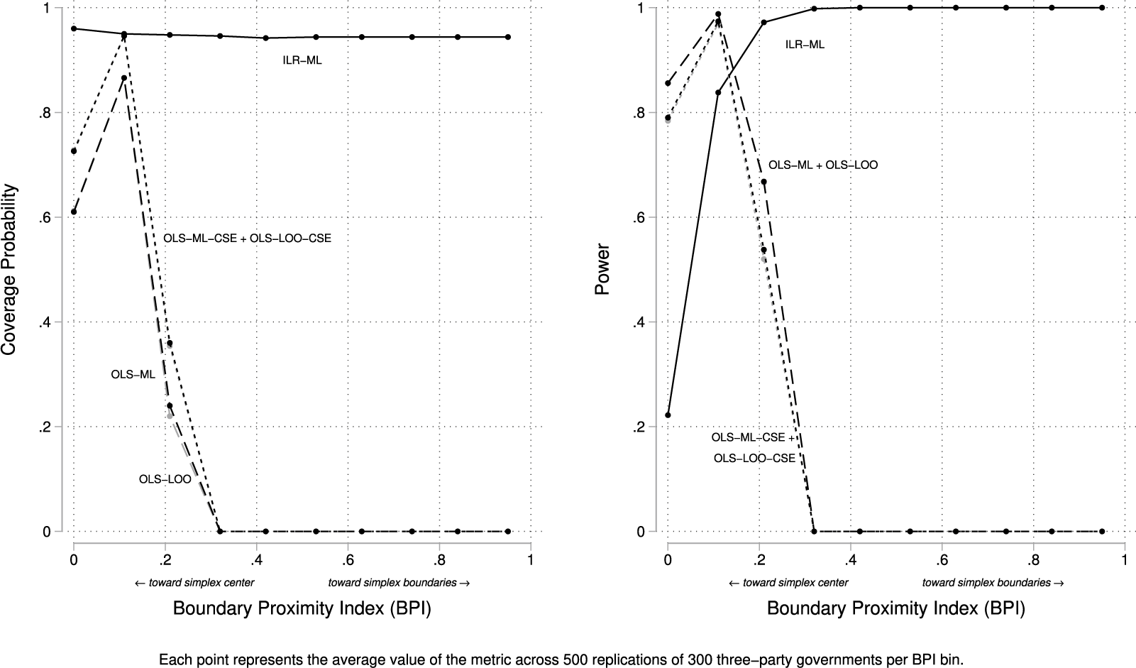
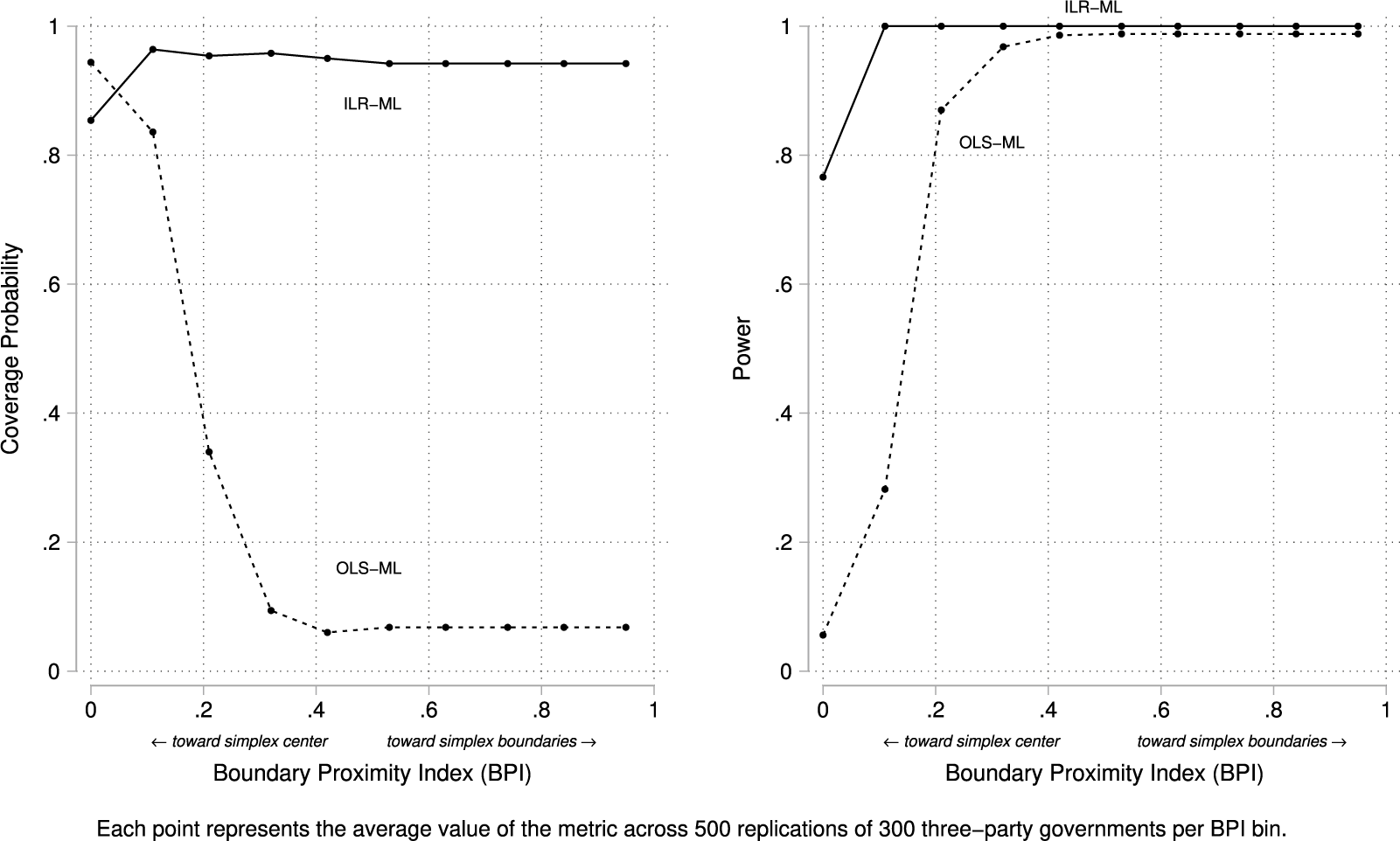
Figure 3 Coverage probability and power ( $H_{0}: \beta \geq 0.80$ ) for $\hat {\beta }$ across BPI.

In Figure 3, we see that coverage probability—the proportion of simulation replications in which the estimator’s confidence interval contains the true value—mirrors this pattern. ILR–ML maintains nominal 95% coverage across the BPI range. By contrast, the OLS estimators collapse almost immediately: once $BPI> 0.20$ , their coverage plunges toward zero, meaning their 95% confidence intervals almost never contain the true slope.

The right panel turns to power. Conventional nulls of $\beta =0$ or $\beta =1$ are uninformative—biased OLS estimates lie far from either, so rejection is trivial. Instead we ask whether models can rule out 5:4 proportionality ( $\beta \ge 0.80$ ), the standard benchmark in the portfolio allocation literature. We define power as the probability that the 95% confidence interval lies entirely below 0.80, i.e., $P(\hat \beta _{U} < 0.80)$ , where $\hat \beta _{U}$ is the 95% upper bound. ILR–ML shows high power across most of the BPI range, whereas OLS estimators rarely reject overly proportional allocations, consistent with their upward bias.Footnote ¹³

4.4 Results for $\hat {\tau }$

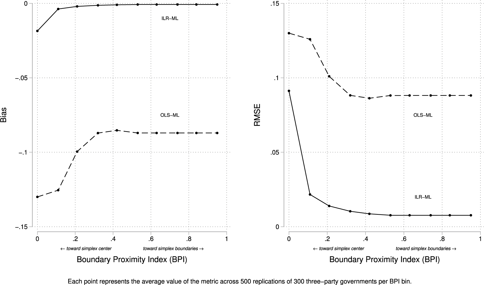
Because variance components are only identifiable in multilevel models, results for $\hat {\tau }$ compare ILR–ML and OLS–ML only (i.e., there is no OLS–LOO analog).Footnote ¹⁴ As shown in Figure 4, ILR–ML successfully recovers slope heterogeneity except at the simplex center, where balanced portfolios provide little signal and mild downward bias appears. RMSE tells the same story, peaking in the center where heterogeneity is hardest to identify, but falling sharply toward the boundaries. OLS–ML, by contrast, consistently estimates $\hat {\tau }$ at or near zero (the assumed true value of $\tau $ minus the estimated bias), producing what looks like low RMSE only because it is systematically wrong. Put differently, ILR–ML recovers slope heterogeneity except at the simplex center, where balanced governments naturally mask variance; OLS–ML misses it everywhere.

Figure 4 Bias and RMSE for $\hat {\tau }$ across BPI.

The coverage probability and power results from Figure 5 confirm this divergence. ILR–ML maintains coverage close to the 95% nominal level, with some erosion at the simplex center where slope heterogeneity is hardest to identify. OLS–ML, by contrast, shows essentially no coverage. Because its variance estimates concentrate at or near zero, the Wald-type confidence intervals are anchored on the boundary and rarely include the true $\tau =0.13$ . This systematic failure is not a matter of random fluctuation, but a structural consequence of misspecified estimation: intervals that collapse at the boundary cannot provide valid coverage for a positive variance component.Footnote ¹⁵

Figure 5 Coverage probability and power ( $H_{0}: \tau = 0$ ) for $\hat {\tau }$ across BPI.

The power test in this case is $H_0\!:\,\tau =0$ . ILR–ML behaves as expected: power is substantial even at the simplex center and quickly approaches one as $BPI$ increases. OLS–ML rises much more slowly: at low $BPI$ , $\hat {\tau }$ piles up at the boundary ( $\approx 0$ ), so the test rarely rejects; once $BPI$ is high enough that OLS returns positive $\hat {\tau }$ , rejection becomes almost automatic. This pattern reflects both misspecification in share space that drives $\hat {\tau }$ to the boundary and the irregular asymptotics of Wald tests for a variance parameter on the boundary (Stram and Lee Reference Stram and Lee1994). Importantly, the coexistence of high apparent power with near-zero coverage implies that OLS rejections do not indicate reliable detection of slope heterogeneity, but rather artifacts of boundary estimation in a misspecified model.

5 Refining Gamson’s Law: Portfolio Allocation in the ILR Framework

Having demonstrated the advantages of the ILR transformation in simulations, we now turn to real-world data to evaluate Gamson’s Law. We draw on the dataset from our previous study (Martin and Vanberg Reference Martin and Vanberg2020), which covers 910 government parties across 308 governments in 16 parliamentary democracies.Footnote ¹⁶ Before presenting the ILR-based analysis, we replicate our earlier findings in Tables 1 and 2.Footnote ¹⁷

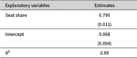
Table 1 Effect of party seat share on share of ministerial posts (single-level OLS–LOO).

Note: Displayed are OLS coefficient estimates, with conventional standard errors in parentheses. Dependent variable: Share of cabinet ministries. N: 602 coalition parties (after 308 parties, one per government, are randomly dropped from the analysis).

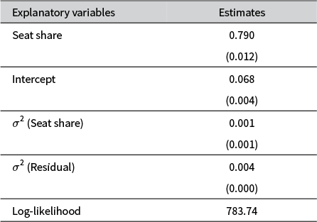
Table 2 Effect of party seat share on share of ministerial posts (multilevel OLS–LOO).

Note: Displayed are maximum likelihood coefficient estimates from a multilevel linear regression, with conventional standard errors in parentheses. The random slope is estimated at the level of the government, and is assumed to be normally distributed. Dependent variable: Share of cabinet ministries. N: 602 coalition parties (after 308 parties, one per government, are randomly dropped from the analysis). The estimated variance of the seat-share slope is effectively zero, and a likelihood-ratio test confirms no improvement over a fixed-slope model ( $\chi ^2 = 1.16, \ p>0.14$ ).

In Table 1, we show the results from the standard (single-level) OLS–LOO model. The estimates confirm what most researchers of portfolio allocation and Gamson’s Law will recognize: an intercept near 0.07, a coefficient on Seat Share close to 0.80, and an $R^2$ of approximately 0.90.Footnote ¹⁸ These results indicate that the relationship between seat share and portfolio share falls short of exact 1:1 proportionality: the intercept differs significantly from zero, and the slope is statistically less than one. Substantively, they suggest a modest numerical “bonus” for small parties and a corresponding “penalty” for large ones—an asymmetry long recognized in the coalition literature (Browne and Franklin Reference Browne and Franklin1973; Warwick and Druckman Reference Warwick and Druckman2006).

We also estimated in our previous study a multilevel (mixed-effects) version of the OLS–LOO model (OLS–ML), which allows the effect of Seat Share to vary across governments. Those findings are reported in Table 2.Footnote ¹⁹ As the results show, the estimated variance of the seat-share slope is close to zero, the likelihood-ratio test fails to reject the null of no heterogeneity ( $p>0.14$ ), and the point estimates are nearly identical to those from the single-level model. In short, the multilevel analysis provides no evidence of variation in the effect of seat share across governments, indicating that the simpler single-level specification in Table 1 fits the data equally well.

But as our simulations make clear, there are strong reasons to doubt the reliability of either specification. Both the single-level and multilevel OLS approaches are structurally misspecified for compositional outcomes: they impose linearity on shares that are bounded and subject to a constant-sum constraint, producing biased point estimates and miscalibrated uncertainty. They also generate predictions that fail to respect compositional coherence.Footnote ²⁰ These deficiencies cast doubt on the apparent stability of the seat–portfolio relationship. What looks like a uniform, law-like association may instead be an artifact of model misspecification. In the analysis that follows, we re-examine the question using the ILR framework, which respects the geometry of compositional data and provides a sounder basis for testing Gamson’s Law.

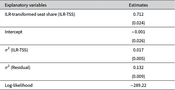
Because our goal is to examine not only the average relationship between seats and portfolios but also the possibility that this effect varies across governments, we estimate a multilevel ILR model, reported in Table 3.Footnote ²¹ The dependent variable is the ILR-Transformed Portfolio Share received by a government party, with the central independent variable defined analogously as the ILR-Transformed Seat Share (ILR-TSS). Because seat shares are themselves compositional, the ILR transformation ensures that changes in a party’s legislative strength are interpreted in relative rather than absolute terms. A one-unit increase in the ILR-TSS represents a proportional gain in that party’s portfolio share relative to the geometric mean of its coalition partners’ shares, not an increase holding others constant.Footnote ²²

Table 3 Effect of party seat share on share of ministerial posts (multilevel ILR).

Note: Displayed are maximum likelihood coefficient estimates from a multilevel linear regression, with conventional standard errors in parentheses. The random slope is estimated at the level of the government, and is assumed to be normally distributed. Dependent variable: Isometric log-ratio (ILR) transformation of numerical share of cabinet ministries. N: 602 balances, reflecting 910 government coalition parties, in 308 governments. A likelihood ratio test of the multilevel ILR model against a single-level ILR alternative leads us to reject the null hypothesis of no difference between them ( $\chi ^2 = 21.82, \ p < 0.001$ ).

To construct these ILR coordinates, we apply an SBP strategy that begins with the smallest party in each government and proceeds in ascending order of seat share. For each party—except the largest—we compare its seat or portfolio share to the geometric mean of the remaining, larger parties, thereby generating a series of balances that contrast smaller parties with blocs of larger coalition partners. The ILR transformation is carried out separately within each government, using only the parties actually present and ordering them consistently by size. This SBP choice is made solely for interpretive clarity; as shown in Appendix 1 of the Supplementary Material, alternative SBPs are linked by orthogonal rotations and yield identical model fit and predictions when mapped back to the simplex.

Because ILR-transformed variables represent log-ratio balances rather than individual proportions, the parameter estimates in Table 3 are not directly interpretable as effects on a single party’s portfolio share. ILR coordinates reflect the log-ratio of one party’s value to the geometric mean of the remaining components in the composition; and under our partitioning strategy, each balance compares a party’s seat share to the geometric mean of the seat shares of all larger coalition partners in the same government. Accordingly, a positive coefficient on ILR-TSS implies that as a party’s seat share increases relative to this geometric mean, its expected portfolio share also increases.

In this context, the model intercept represents the expected portfolio balance when the logged seat-share balance is zero—that is, when a party’s seat share is exactly equal to the geometric mean of the seat shares of its larger partners. The estimated intercept is close to zero and not statistically distinguishable from it ( $p \approx 0.98$ ). Substantively, this suggests that when a party is perfectly balanced in legislative size relative to its larger partners, it receives a proportionate share of cabinet portfolios. There is no systematic upward or downward shift at this point of balance.Footnote ²³

Turning to the average slope, the coefficient on ILR–TSS is positive and highly significant, but its magnitude—0.71—is well below one, indicating that the relationship between seat share and portfolio share is less than perfectly proportional. To facilitate comparison with the OLS estimate in share space, we approximate the corresponding proportionality by taking the ratio of exponentiated coefficients, e ^0.71/e ¹ ≈ 0.75. This suggests that a proportional 4% increase in seat share corresponds, on average, to only about a 3% increase in portfolio share. The effect is notably smaller—and statistically different ( $p<0.001$ )—than the 5:4 proportionality estimated using OLS on untransformed data. In short, while the association between seats and portfolios remains strong, it is weaker than previously thought.

This conclusion also revises our earlier finding in Martin and Vanberg (Reference Martin and Vanberg2020)—based on an OLS model using untransformed shares—that the effect of seat share on portfolio share is homogeneous across governments. That earlier result now appears to reflect a limitation of the OLS framework rather than a feature of the underlying data. As shown in our Monte Carlo simulations, linear models applied to raw compositional outcomes impose a misspecified error structure that can mask true heterogeneity, either through biased point estimates or distorted uncertainty estimates. By contrast, modeling the data in ILR space respects its compositional structure and reveals variation in the seat-to-portfolio relationship that is substantively meaningful but previously hidden.

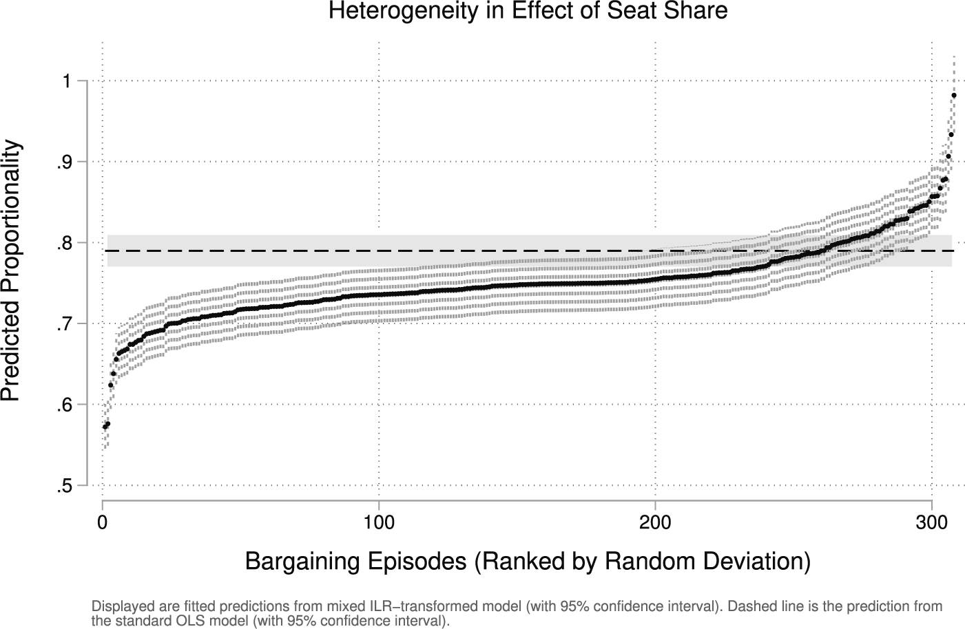
The multilevel ILR model indeed uncovers such heterogeneity. The variance component of ILR-TSS indicates that the strength of the seat-to-portfolio relationship varies across governments. Using best linear unbiased predictions (BLUPs) of the random slope deviations, we calculate predicted seat share coefficients for each of the 308 governments. Figure 6 displays these coefficients (with 95% confidence intervals), ordered by magnitude. To facilitate direct comparison with the fixed coefficient estimate from the conventional OLS model (Table 1), we again transform the ILR-based slope estimates back to the original share metric by exponentiating each value and dividing by the exponentiated value of one (corresponding to perfect proportionality). This places them on the same scale as the OLS coefficient and allows us to assess how proportionality varies across governments. As a benchmark, the figure overlays the OLS slope and its confidence interval. While this OLS estimate treats the slope as uniform across cases, the ILR estimates show otherwise: 148 of the 308 government-specific slopes fall significantly below the OLS estimate ( $p < 0.05$ ), while 17 fall significantly above it. The wide dispersion underscores the value of the ILR-based multilevel approach in capturing variation that conventional methods obscure.Footnote ²⁴

Figure 6 Heterogeneity in effect of seat share.

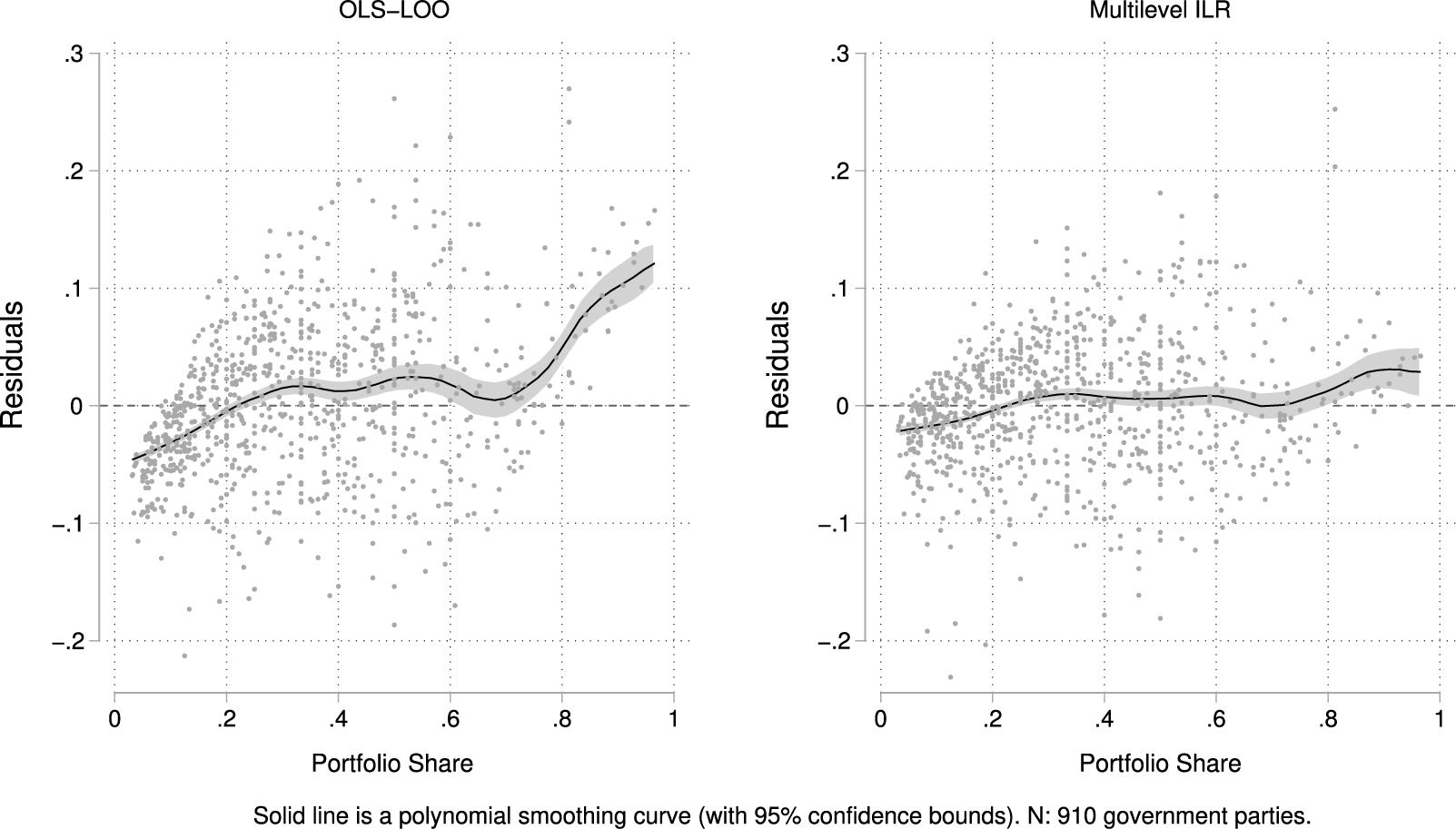
Beyond uncovering heterogeneity, the ILR model also fits the data far better than the conventional OLS model—a point made clear by comparing residual patterns between the two. If both models effectively capture the underlying dynamics, we should observe no systematic relationship between residuals and the (untransformed) variable of interest, Portfolio Share. To assess this, we calculate predicted values from each model. For OLS, this is straightforward. For the ILR model, predictions are made in log-ratio space and then back-transformed to the compositional scale.Footnote ²⁵ Residuals are then calculated as the difference between observed and predicted portfolio shares.

Figure 7 provides a visual comparison of residuals from the conventional OLS model and the ILR-based multilevel model. The contrast is striking. In the OLS model, residuals exhibit pronounced curvature—the mean reflected in the polynomial smoothing curve is rarely centered at zero—with systematic overprediction at the low end of the distribution and underprediction at the high end.Footnote ²⁶ This pattern reflects the inherent limitations of applying linear regression to compositional outcomes: the model imposes a linear structure on data constrained to a simplex, leading to distortion—especially near the boundaries. By contrast, residuals from the ILR model are much more evenly distributed around zero, with little curvature and substantially reduced magnitude. While some misprediction persists at the extremes, it is markedly diminished—particularly at the upper end of the distribution, where the OLS model performs worst. The visual contrast is matched by a substantial difference in fit: the residual sum of squares in the OLS model is 56% higher than in the ILR model. Together, these results reinforce the argument that OLS imposes a misspecified structure on portfolio data, obscuring underlying patterns. The ILR framework not only reveals heterogeneity in effects but also yields more accurate and statistically coherent estimates across the board.

Figure 7 Residual patterns: Conventional OLS versus multilevel ILR.

6 Discussion and Conclusion

Our analyses indicate that the apparent stability of the seat–portfolio link rests on methods not appropriate for modeling compositional outcomes. Because portfolio and seat shares are parts of a whole, their interdependence and bounded support violate key assumptions of conventional linear models. The Monte Carlo evidence shows these violations are not benign: across a wide range of conditions, OLS estimators produce systematic bias, low power, and sharply degraded coverage once allocations move away from the simplex center. Even in multilevel form, OLS struggles to recover genuine random-slope variation. In short, part of what earlier studies treated as a “law-like” regularity reflects model misspecification rather than true stability. By contrast, the ILR transformation estimated in a multilevel framework aligns the model with the geometry of the data. In the simulations, ILR–ML accurately recovers the mean proportionality parameter, with high power and near-nominal coverage throughout the simplex. It also identifies random-slope variance that OLS largely obscures.

Applied to real-world coalition data, the ILR model revises the standard picture. The average relationship between seat share and portfolio share is weaker than the canonical 5:4 estimate, closer to 4:3. This implies that small parties receive larger portfolio rewards relative to their legislative strength than previously recognized. Just as important, the effect of seat share is not constant across governments: ILR–ML uncovers wide dispersion in slopes, indicating that proportionality is contingent on features of specific bargaining episodes. Some governments approach near-perfect proportionality, while others deviate sharply from it. This pattern accords with our residual comparison, where the ILR model eliminates much of the curvature and magnitude seen under OLS. Substantively, these findings suggest that Gamson’s “law” is better viewed as a central tendency that strengthens or weakens with context. The ILR framework provides a way to investigate those contexts directly.

Methodologically, the implications extend well beyond portfolio allocation. Many political outcomes are compositional and differ in which components are observed across cases: party vote shares when not all parties compete in every district, media attention when the set of salient policy issues changes over time or across countries, or public spending shares when budget categories are redefined or reorganized. In such settings, ALR+SUR is often infeasible because it requires a fixed set of components and a stable reference part across all observations. The ILR transformation avoids these constraints by adapting to the observed composition within each unit while preserving the geometry of the simplex. As researchers model outcomes that represent divisions of finite resources, ILR offers a practical way to reduce bias and achieve more reliable inference.