

1 INTRODUCTION
Empirical research investigating network formation and outcomes spans the literature covering labor economics, industrial organization, macroeconomics, development, and international trade, among others. In a large fraction of these studies, the process through which entities are determined—e.g., free/preferential trade agreements, friendships, and financial relationships—concerns dyadic/network link formation models. While recent methodological advances have increased the popularity of empirical network formation models (see Graham (Reference Graham2020) and Graham and de Paula (Reference Graham and de Paula2020) for surveys), the large majority of existing studies focus on parsimonious (low-dimensional) model specifications. The increasing availability of “big data” should, in principle, allow researchers to consider increasingly rich specifications and uncover new insights into the nature of network formation. Rather, researchers are hamstrung by two competing limitations. On the one hand, there is no existing statistical methodology that allows for both dyadic robust inference and high-dimensional link formation specifications. In the presence of significant data heterogeneity in the policy variable of interest, one needs to control a large number of covariates. However, simply estimating a rich specification across a wide set of covariates is not yet possible. Moreover, we document that common off-the-shelf approaches, such as the conventional double/debiased machine learning (DML) for i.i.d. sampling, are likely to result in both biased estimates and misleading standard errors under dyadic dependence. On the other hand, the most common empirical approach, reducing the dimensionality of the network formation model by assumption, risks model misspecification, is a likely source of estimation bias and/or misleading inference, and reduces the set of questions researchers can investigate. In light of the increasing availability of big data today, we advance state-of-the-art approaches to estimating network models by developing novel methods for root-n consistent estimation and inference for high-dimensional dyadic regressions and high-dimensional dyadic/network link formation models.
Our work builds on the literature which suggests using (near) Neyman orthogonal scores to accommodate possibly slow convergence rates of general machine learners (e.g., Belloni et al. Reference Belloni, Chernozhukov and Kato2015, Belloni et al., Reference Belloni, Chernozhukov, Chetverikov and Wei2018, Chernozhukov et al. Reference Chernozhukov, Chetverikov, Demirer, Duflo, Hansen, Newey and Robins2018, Reference Chernozhukov, Escanciano, Ichimura, Newey and Robins2022) in high-dimensional regression estimation (and more generally semiparametric Z-estimation). In particular, our approach extends the branch of research which employs cross-fitting, in conjunction with orthogonal scores, to mitigate over-fitting biases. This combined method is referred to as DML (Chernozhukov et al. Reference Chernozhukov, Chetverikov, Demirer, Duflo, Hansen, Newey and Robins2018).
Standard DML requires independent sampling. In a recent work, Chiang et al. (Reference Chiang, Kato, Ma and Sasaki2022) develop a multiway cross-fitting algorithm to extend the DML to multiway cluster dependent data with linear scores. Although conceptually related, the methodology in this article differs fundamentally from Chiang et al. (Reference Chiang, Kato, Ma and Sasaki2022) in two respects. First, Chiang et al. (Reference Chiang, Kato, Ma and Sasaki2022) does not permit the estimation of network models in the presence of dyadic dependence. Dyadic dependence is different from (multiway) cluster dependence,Footnote 1 and hence the existing cross-fitting algorithms are not guaranteed to work for dyadic regressions and dyadic/network link formation models. In this light, we propose a novel cross-fitting algorithm that is effective under dyadic dependence. Second, Chiang et al. (Reference Chiang, Kato, Ma and Sasaki2022) do not cover estimators defined by nonlinear scores, such as Logit. Coping with such nonlinear structures presents extra theoretical challenges as it demands tight control of the stochastic magnitude of various empirical processes under dyadic dependence. Our dyadic machine learning approach and asymptotic theories cover a large class of general nonlinear estimation problems and guarantee that estimation and inference based on this method are robust against arbitrary dyadic dependence. See Appendix I of the Supplementary Material for further details.
Relation to the Literature: Due to space constraints, a comprehensive literature review is provided in Appendix H of the Supplementary Material.
2 THE DYADIC DOUBLE/DEBIASED MACHINE LEARNING
In this section, we introduce the model and present our proposed method of dyadic machine learning. A theoretical guarantee that this method works will be presented in Section 3. We start by fixing notations to be used to describe dyadic data. Assume that a dyadic sample contains N nodes with no self-links. For any $r\in \mathbb {N}$
, let
$r\in \mathbb {N}$
, let $[r]=\{1,\ldots , r\}$
. For any finite set I with
$[r]=\{1,\ldots , r\}$
. For any finite set I with $I\subset [N]$
, we use the “bar-square” notation to denote the set of two-tuples of I without repetition, i.e.,
$I\subset [N]$
, we use the “bar-square” notation to denote the set of two-tuples of I without repetition, i.e., $\overline {I^2}=\{(i,j)\in I\times I: i\neq j\}$
. A dyadic observation is written as
$\overline {I^2}=\{(i,j)\in I\times I: i\neq j\}$
. A dyadic observation is written as $W_{ij}$
for
$W_{ij}$
for $(i,j)\in \overline {\mathbb {N}^{+2}}$
, where
$(i,j)\in \overline {\mathbb {N}^{+2}}$
, where $\mathbb {N}^+$
represents the set of positive integers, and we assume that this random vector
$\mathbb {N}^+$
represents the set of positive integers, and we assume that this random vector $W_{ij}$
is Borel measurable throughout.Footnote
2
We assume the identical distribution of
$W_{ij}$
is Borel measurable throughout.Footnote
2
We assume the identical distribution of $W_{ij}$
. Let
$W_{ij}$
. Let $\{\mathcal P_{N}\}_{N}$
be a sequence of sets of probability laws of
$\{\mathcal P_{N}\}_{N}$
be a sequence of sets of probability laws of $\{W_{ij}\}{}_{ij}$
, let
$\{W_{ij}\}{}_{ij}$
, let $P=P_{N}\in \mathcal {P}{}_{N}$
denote the law with the sample size N, and let
$P=P_{N}\in \mathcal {P}{}_{N}$
denote the law with the sample size N, and let $\mathrm {E}_{P}$
denote the expectation with respect to P. We write the dyadic sample expectation operator by
$\mathrm {E}_{P}$
denote the expectation with respect to P. We write the dyadic sample expectation operator by $\mathbb {E}_{_NC_2}[\cdot ]=\frac {1}{N(N-1)}\sum \limits _{(i,j) \in \overline {[N]^2}} [\cdot ]$
. For any finite set I with
$\mathbb {E}_{_NC_2}[\cdot ]=\frac {1}{N(N-1)}\sum \limits _{(i,j) \in \overline {[N]^2}} [\cdot ]$
. For any finite set I with $I\subset [N]$
, we let
$I\subset [N]$
, we let $|I|$
denote the cardinality of I, and let
$|I|$
denote the cardinality of I, and let $I^c$
denote the complement of I, namely,
$I^c$
denote the complement of I, namely, $I^c=[N]\setminus I$
. We write the dyadic subsample expectation operator by
$I^c=[N]\setminus I$
. We write the dyadic subsample expectation operator by $\mathbb {E}{}_{{}_{|I|}C{}_2}[\cdot ]:=\frac {1}{|I|(|I|-1)}\sum _{(i,j)\in \overline {I^2}}[\cdot ]$
.
$\mathbb {E}{}_{{}_{|I|}C{}_2}[\cdot ]:=\frac {1}{|I|(|I|-1)}\sum _{(i,j)\in \overline {I^2}}[\cdot ]$
.
2.1 The Model
The economic model is assumed to satisfy the moment restriction
 $$ \begin{align} \mathrm{E}_{P}[\psi(W_{ij};\theta_0,\eta_0)]=0 \end{align} $$
for some score function $\psi $
that depends on a low-dimensional parameter vector
$\psi $
that depends on a low-dimensional parameter vector ![]() and a nuisance parameter
and a nuisance parameter $\eta \in T$
for a convex set T. The nuisance parameter
$\eta \in T$
for a convex set T. The nuisance parameter $\eta $
may be finite-, high-, or infinite-dimensional. The true values of
$\eta $
may be finite-, high-, or infinite-dimensional. The true values of $\theta $
and
$\theta $
and $\eta $
are denoted by
$\eta $
are denoted by $\theta _0 \in \Theta $
and
$\theta _0 \in \Theta $
and $\eta _0 \in T$
, respectively.
$\eta _0 \in T$
, respectively.
Let $\widetilde T=\{\eta - \eta _0 : \eta \in T\}$
, and define the Gâteaux derivative map
$\widetilde T=\{\eta - \eta _0 : \eta \in T\}$
, and define the Gâteaux derivative map ![]() by
by $ D_r[\eta -\eta _0]:=\partial _r \Big \{ \mathrm {E}_{P}[\psi (W_{ij};\theta _0,\eta _0+r(\eta -\eta _0))]\Big \} $
for all
$ D_r[\eta -\eta _0]:=\partial _r \Big \{ \mathrm {E}_{P}[\psi (W_{ij};\theta _0,\eta _0+r(\eta -\eta _0))]\Big \} $
for all $r\in [0,1)$
. Let its limit, as
$r\in [0,1)$
. Let its limit, as $r\rightarrow 0$
, be denoted by
$r\rightarrow 0$
, be denoted by $ \partial _\eta \mathrm {E}_{P}\psi (W_{ij};\theta _0,\eta _0)[\eta - \eta _0]:=D_0[\eta -\eta _0]. $
We say that the Neyman orthogonality condition holds at
$ \partial _\eta \mathrm {E}_{P}\psi (W_{ij};\theta _0,\eta _0)[\eta - \eta _0]:=D_0[\eta -\eta _0]. $
We say that the Neyman orthogonality condition holds at $(\theta _0,\eta _0)$
with respect to a nuisance realization set
$(\theta _0,\eta _0)$
with respect to a nuisance realization set $\mathcal T{}_N \subset T$
if the score
$\mathcal T{}_N \subset T$
if the score $\psi $
satisfies (2.1), the pathwise derivative
$\psi $
satisfies (2.1), the pathwise derivative ${D_r[\eta -\eta _0]}$
exists for all
${D_r[\eta -\eta _0]}$
exists for all $r\in [0,1)$
and
$r\in [0,1)$
and $\eta \in \mathcal T{}_N$
, and the orthogonality equation
$\eta \in \mathcal T{}_N$
, and the orthogonality equation
 $$ \begin{align} \partial_\eta\mathrm{E}_{P}\psi(W_{ij};\theta_0,\eta_0)[\eta - \eta_0]=0 \end{align} $$
holds for all $\eta \in \mathcal T_N$
. Furthermore, we also say that the
$\eta \in \mathcal T_N$
. Furthermore, we also say that the $\lambda _N$
Neyman near-orthogonality condition holds at
$\lambda _N$
Neyman near-orthogonality condition holds at $(\theta _0,\eta _0)$
with respect to a nuisance realization set
$(\theta _0,\eta _0)$
with respect to a nuisance realization set $\mathcal T_N\subset T$
if the score
$\mathcal T_N\subset T$
if the score $\psi $
satisfies (2.1), the pathwise derivative
$\psi $
satisfies (2.1), the pathwise derivative ${D_r[\eta -\eta _0]}$
exists for all
${D_r[\eta -\eta _0]}$
exists for all $r\in [0,1)$
and
$r\in [0,1)$
and $\eta \in \mathcal T_N$
, and the orthogonality equation
$\eta \in \mathcal T_N$
, and the orthogonality equation
 $$ \begin{align} \sup_{\eta \in \mathcal T_N}\Big\| \partial_\eta \mathrm{E}_{P}\psi(W_{ij};\theta_0,\eta_0)[\eta-\eta_0] \Big\|\le \lambda_N \end{align} $$
holds for all $\eta \in \mathcal T_N$
for some positive sequence
$\eta \in \mathcal T_N$
for some positive sequence $\{\lambda _N\}_N$
such that
$\{\lambda _N\}_N$
such that $\lambda _N=o(N^{-1/2})$
. We refer readers to Chernozhukov et al. (Reference Chernozhukov, Chetverikov, Demirer, Duflo, Hansen, Newey and Robins2018) for detailed discussions of the Neyman (near) orthogonality, including its intuitions and a general procedure to construct scores
$\lambda _N=o(N^{-1/2})$
. We refer readers to Chernozhukov et al. (Reference Chernozhukov, Chetverikov, Demirer, Duflo, Hansen, Newey and Robins2018) for detailed discussions of the Neyman (near) orthogonality, including its intuitions and a general procedure to construct scores $\psi $
satisfying it.
$\psi $
satisfying it.
Throughout, we will consider structural models satisfying the moment restriction (2.1) and either form of the Neyman orthogonality conditions, (2.2) or (2.3). As a concrete motivating example of the above abstract formulation, Example 1 below presents the logit dyadic link formation models, which we consider for our main application in this article. In addition, we also present a couple of simpler examples with the linear regression models and the linear IV regression models in Appendix A.1 of the Supplementary Material.
Example 1 (Logit Dyadic Link Formation Models).
Let $W_{ij}=(Y_{ij},D_{ij},X_{ij}')'$
, where
$W_{ij}=(Y_{ij},D_{ij},X_{ij}')'$
, where $Y_{ij}$
is a binary indicator for a link formed between nodes i and j,
$Y_{ij}$
is a binary indicator for a link formed between nodes i and j, $D_{ij}$
is an explanatory variable of interest, and
$D_{ij}$
is an explanatory variable of interest, and $X_{ij}$
is a high-dimensional random vector of controls. Consider the logistic dyadic link formation model
$X_{ij}$
is a high-dimensional random vector of controls. Consider the logistic dyadic link formation model
 $$ \begin{align*} \mathrm{E}_{P}[Y_{ij}|D_{ij},X_{ij}]=\Lambda(D_{ij}\theta_0 + X_{ij}'\beta_0) \text{ for }(i,j)\in \overline{[N]^2}, \end{align*} $$
where $\theta $
is a scalar parameter of interest,Footnote
3
$\theta $
is a scalar parameter of interest,Footnote
3 $\beta $
is a nuisance parameter, and
$\beta $
is a nuisance parameter, and $\Lambda (t)=\exp (t)/(1+\exp (t))$
for all
$\Lambda (t)=\exp (t)/(1+\exp (t))$
for all ![]() . A nonlinear Neyman orthogonal score
. A nonlinear Neyman orthogonal score $\psi $
in this model is given by
$\psi $
in this model is given by
 $$ \begin{align*}\psi(W_{ij};\theta,\eta)=\{Y_{ij}-\Lambda(D_{ij}\theta+X_{ij}'\beta)\}(D_{ij}-X_{ij}' \gamma), \end{align*} $$
where $\eta = (\beta ',\gamma ')'$
with
$\eta = (\beta ',\gamma ')'$
with $\gamma $
denoting the coefficients of a weighted projection of
$\gamma $
denoting the coefficients of a weighted projection of $D_{ij}$
on
$D_{ij}$
on $X_{ij}$
. See Section 4 for more details about this example as well as our general theory applied to this example.
$X_{ij}$
. See Section 4 for more details about this example as well as our general theory applied to this example.
2.2 Dyadic Cross-Fitting
For the class of models introduced in Section 2.1, we now propose a novel dyadic cross-fitting procedure for estimation of $\theta _0$
. With a fixed positive integer K, randomly partition the set
$\theta _0$
. With a fixed positive integer K, randomly partition the set $[N] = \{1,\ldots ,N\}$
of indices of N nodes into K parts
$[N] = \{1,\ldots ,N\}$
of indices of N nodes into K parts $\{I_1,\ldots ,I_K\}$
. For each
$\{I_1,\ldots ,I_K\}$
. For each $k \in [K] = \{1,\ldots ,K\}$
, obtain an estimate
$k \in [K] = \{1,\ldots ,K\}$
, obtain an estimate
 $$ \begin{align*}\widehat \eta_{k}=\widehat \eta\left((W_{ij})_{(i,j)\in \overline{([N]\setminus I_k )^2}}\right)\end{align*} $$
of the nuisance parameter $\eta $
by a machine learning method (e.g., lasso, post-lasso, elastic nets, ridge, deep neural networks, and boosted trees) using only the subsample of those observations with dyadic indices
$\eta $
by a machine learning method (e.g., lasso, post-lasso, elastic nets, ridge, deep neural networks, and boosted trees) using only the subsample of those observations with dyadic indices $(i,j)$
in
$(i,j)$
in $\overline {([N]\setminus I_k )^2}$
. In turn, we define the dyadic machine learning estimator
$\overline {([N]\setminus I_k )^2}$
. In turn, we define the dyadic machine learning estimator $\widetilde \theta $
for
$\widetilde \theta $
for $\theta _0$
as the solution to
$\theta _0$
as the solution to
 $$ \begin{align} \frac{1}{K}\sum\limits_{k \in [K]} \mathbb{E}_{_{|I_k|}C_2}[\psi(W;\widetilde \theta,\widehat \eta_{k})] =0, \end{align} $$
where we recall that $\mathbb {E}_{_{|I_k|}C_2} [f(W)] = \frac {1}{|I_k|(|I_k|-1)}\sum _{(i,j)\in \overline {I_k^2}} f(W_{ij})$
denotes the subsample empirical expectation using only those observations with dyadic indices
$\mathbb {E}_{_{|I_k|}C_2} [f(W)] = \frac {1}{|I_k|(|I_k|-1)}\sum _{(i,j)\in \overline {I_k^2}} f(W_{ij})$
denotes the subsample empirical expectation using only those observations with dyadic indices $(i,j)$
in
$(i,j)$
in $\overline {I_k ^2}$
. If an achievement of the exact 0 is not possible as in (2.4), then one may define the estimator
$\overline {I_k ^2}$
. If an achievement of the exact 0 is not possible as in (2.4), then one may define the estimator $\widetilde {\theta }$
as an approximate
$\widetilde {\theta }$
as an approximate $\epsilon _N$
-solution:
$\epsilon _N$
-solution:
 $$ \begin{align} \left\| \frac{1}{K} \sum\limits_{k \in [K]} \mathbb{E}_{_{|I_k|}C_2}[\psi(W; \widetilde{\theta}, \widehat{\eta}_{k})]\right\| \leq \inf _{\theta \in \Theta}\left\| \frac{1}{K} \sum\limits_{k \in [K]} \mathbb{E}_{_{|I_k|}C_2}\left[\psi\left(W; \theta, \widehat{\eta}_{ k}\right)\right] \right\|+\epsilon_{N}, \end{align} $$
where $\epsilon _N=o(\delta _N N^{-1/2})$
and restrictions on the sequence
$\epsilon _N=o(\delta _N N^{-1/2})$
and restrictions on the sequence $\{\delta _N\}_N$
will be formally discussed in Section 3. Under the assumptions to be introduced in Section 3, this dyadic machine learning estimator
$\{\delta _N\}_N$
will be formally discussed in Section 3. Under the assumptions to be introduced in Section 3, this dyadic machine learning estimator $\widetilde \theta $
enjoys the root-N asymptotic normality
$\widetilde \theta $
enjoys the root-N asymptotic normality $ \sqrt {N}\sigma ^{-1}(\widetilde \theta - \theta _0) \leadsto N(0,I_{d_\theta }), $
where a concrete expression for the asymptotic variance
$ \sqrt {N}\sigma ^{-1}(\widetilde \theta - \theta _0) \leadsto N(0,I_{d_\theta }), $
where a concrete expression for the asymptotic variance $\sigma ^2$
will be presented in Theorem 1 ahead.
$\sigma ^2$
will be presented in Theorem 1 ahead.
Note that, for each $k\in [K]$
, the nuisance parameter estimator
$k\in [K]$
, the nuisance parameter estimator $\widehat \eta _{k}$
is computed using the subsample of those observations with dyadic indices
$\widehat \eta _{k}$
is computed using the subsample of those observations with dyadic indices $(i,j) \in \overline { ([N]\setminus I_k )^2} $
, and in turn, the average score
$(i,j) \in \overline { ([N]\setminus I_k )^2} $
, and in turn, the average score $\mathbb {E}_{_{|I_k|}C_2}[\psi (W; \cdot ,\widehat \eta _{k})]$
is computed using the subsample of those observations with dyadic indices
$\mathbb {E}_{_{|I_k|}C_2}[\psi (W; \cdot ,\widehat \eta _{k})]$
is computed using the subsample of those observations with dyadic indices $(i,j) \in \overline { I_k ^2}$
. This two-step computation is repeated K times. We call this cross-fitting procedure the K-fold dyadic cross-fitting. It differs from and complements the cross-fitting procedure of Chernozhukov et al. (Reference Chernozhukov, Chetverikov, Demirer, Duflo, Hansen, Newey and Robins2018) for i.i.d. data and the cross-fitting procedure of Chiang et al. (Reference Chiang, Kato, Ma and Sasaki2022) for multiway clustered data—neither of these existing cross-fitting methods will work under dyadic dependence. If the dyadic sample
$(i,j) \in \overline { I_k ^2}$
. This two-step computation is repeated K times. We call this cross-fitting procedure the K-fold dyadic cross-fitting. It differs from and complements the cross-fitting procedure of Chernozhukov et al. (Reference Chernozhukov, Chetverikov, Demirer, Duflo, Hansen, Newey and Robins2018) for i.i.d. data and the cross-fitting procedure of Chiang et al. (Reference Chiang, Kato, Ma and Sasaki2022) for multiway clustered data—neither of these existing cross-fitting methods will work under dyadic dependence. If the dyadic sample $\{W_{ij}\}_{ij}$
would reduce to the monadic sample
$\{W_{ij}\}_{ij}$
would reduce to the monadic sample $\{W_i\}_i$
, then the K-fold dyadic cross-fitting would accordingly boil down to the K-fold cross-fitting procedure of Chernozhukov et al. (Reference Chernozhukov, Chetverikov, Demirer, Duflo, Hansen, Newey and Robins2018).
$\{W_i\}_i$
, then the K-fold dyadic cross-fitting would accordingly boil down to the K-fold cross-fitting procedure of Chernozhukov et al. (Reference Chernozhukov, Chetverikov, Demirer, Duflo, Hansen, Newey and Robins2018).
Figure 1 illustrates the dyadic cross-fitting for the case of $K=2$
. We let
$K=2$
. We let $N=8$
for simplicity of illustration, although actual sample sizes should be much larger. Suppose that a random partition of
$N=8$
for simplicity of illustration, although actual sample sizes should be much larger. Suppose that a random partition of $[8] = \{1,\ldots ,8\}$
entails two folds with one consisting of
$[8] = \{1,\ldots ,8\}$
entails two folds with one consisting of $I_1 = \{1,\ldots ,4\}$
and the other consisting of
$I_1 = \{1,\ldots ,4\}$
and the other consisting of $I_2 = \{5,\ldots ,8\}$
. In the left panel, we compute
$I_2 = \{5,\ldots ,8\}$
. In the left panel, we compute $\widehat \eta _1$
with a machine learner applied to the subsample
$\widehat \eta _1$
with a machine learner applied to the subsample $\overline {(I_1^c)^2}$
marked by “Nuisance” in the gray shades at the bottom right quarter of the grid, and then evaluate the subsample mean
$\overline {(I_1^c)^2}$
marked by “Nuisance” in the gray shades at the bottom right quarter of the grid, and then evaluate the subsample mean $\mathbb {E}_{_{|I_1|}C_2}[\psi (W;\widetilde \theta ,\widehat \eta _{1})]$
of the score using the subsample
$\mathbb {E}_{_{|I_1|}C_2}[\psi (W;\widetilde \theta ,\widehat \eta _{1})]$
of the score using the subsample $\overline {I_1^2}$
marked by “Score” in the gray shades at the top left quarter of the grid. In the right panel, in turn, we compute
$\overline {I_1^2}$
marked by “Score” in the gray shades at the top left quarter of the grid. In the right panel, in turn, we compute $\widehat \eta _2$
with a machine learner applied to the subsample
$\widehat \eta _2$
with a machine learner applied to the subsample $\overline {(I_2^c)^2}$
marked by “Nuisance” in the gray shades at the top left quarter of the grid, and then evaluate the subsample mean
$\overline {(I_2^c)^2}$
marked by “Nuisance” in the gray shades at the top left quarter of the grid, and then evaluate the subsample mean $\mathbb {E}_{_{|I_2|}C_2}[\psi (W;\widetilde \theta ,\widehat \eta _{2})]$
of the score using the subsample
$\mathbb {E}_{_{|I_2|}C_2}[\psi (W;\widetilde \theta ,\widehat \eta _{2})]$
of the score using the subsample $\overline {I_2^2}$
marked by “Score” in the gray shades at the bottom right quarter of the grid. Although the figure may apparently suggest as if we were discarding the information in the off-diagonal half of the dyad, our dyadic machine learning method uses the full information of N nodes for estimation of
$\overline {I_2^2}$
marked by “Score” in the gray shades at the bottom right quarter of the grid. Although the figure may apparently suggest as if we were discarding the information in the off-diagonal half of the dyad, our dyadic machine learning method uses the full information of N nodes for estimation of $\theta $
. Specifically, this means that Equation (2.4) evaluates the score with all of the N nodes (see Equation (3.3) ahead for a precise mathematical expression in support of this argument). The white off-diagonal blocks reflect that the
$\theta $
. Specifically, this means that Equation (2.4) evaluates the score with all of the N nodes (see Equation (3.3) ahead for a precise mathematical expression in support of this argument). The white off-diagonal blocks reflect that the $(K-1)/K$
fraction of data are used to estimate the nuisance parameter
$(K-1)/K$
fraction of data are used to estimate the nuisance parameter $\eta _k$
for each
$\eta _k$
for each $k \in [K]$
, but this will not affect the asymptotic behavior of the estimator
$k \in [K]$
, but this will not affect the asymptotic behavior of the estimator $\widetilde \theta $
of interest due to the Neyman orthogonality, as is the case with the conventional DML of Chernozhukov et al. (Reference Chernozhukov, Chetverikov, Demirer, Duflo, Hansen, Newey and Robins2018). As a matter of fact, the next section shows that our estimator
$\widetilde \theta $
of interest due to the Neyman orthogonality, as is the case with the conventional DML of Chernozhukov et al. (Reference Chernozhukov, Chetverikov, Demirer, Duflo, Hansen, Newey and Robins2018). As a matter of fact, the next section shows that our estimator $\widetilde \theta $
achieves the root-N asymptotic normality with the asymptotic variance being the same as the one in the case where an oracle would let us know the true nuisance parameter
$\widetilde \theta $
achieves the root-N asymptotic normality with the asymptotic variance being the same as the one in the case where an oracle would let us know the true nuisance parameter $\eta $
.
$\eta $
.
An illustration of the $2$
-fold dyadic cross-fitting.
$2$
-fold dyadic cross-fitting.

Remark 1. In the context of dyadic data, the first-order asymptotic distribution is governed by information at the individual (node) level rather than at the dyad (pair) level. This is consistent with the convergence rate in dyadic asymptotics being root-N, as opposed to root- $N(N-1)$
, reflecting that the effective sample size is determined by the number of nodes. Although estimation utilizes dyadic pairs, the leading influence function terms depend on node-specific information. Consequently, the fact that some dyadic pairs are excluded from particular folds during cross-fitting does not result in a first-order efficiency loss.
$N(N-1)$
, reflecting that the effective sample size is determined by the number of nodes. Although estimation utilizes dyadic pairs, the leading influence function terms depend on node-specific information. Consequently, the fact that some dyadic pairs are excluded from particular folds during cross-fitting does not result in a first-order efficiency loss.
Remark 2 (Unbalanced dyads).
We now consider the case of unbalanced dyads. For simplicity, let us focus on the case of undirected dyadic data, that is, dyads indexed by pairs with $ i < j $
. Suppose the data are unbalanced in the sense that we only observe dyads
$ i < j $
. Suppose the data are unbalanced in the sense that we only observe dyads $(i,j)$
for
$(i,j)$
for $ i = 1, \ldots , N $
and
$ i = 1, \ldots , N $
and $ j = 1, \ldots , M $
, where
$ j = 1, \ldots , M $
, where $ N < M $
, and both
$ N < M $
, and both $ N $
and
$ N $
and $ M $
diverge proportionally. The proposed method continues to apply in this setting, with the only required modification being an appropriate adjustment to the effective sample size. In such cases, we recommend using all available dyads rather than restricting attention to a balanced subset of
$ M $
diverge proportionally. The proposed method continues to apply in this setting, with the only required modification being an appropriate adjustment to the effective sample size. In such cases, we recommend using all available dyads rather than restricting attention to a balanced subset of $ N\choose 2 $
observations. Retaining the full set of dyads yields an asymptotic variance that lies between
$ N\choose 2 $
observations. Retaining the full set of dyads yields an asymptotic variance that lies between $ \frac {1}{4} $
and
$ \frac {1}{4} $
and $ 1 $
times the variance in the balanced design, and hence can lead to efficiency gains.
$ 1 $
times the variance in the balanced design, and hence can lead to efficiency gains.
3 THEORY
In this section, we present a formal theory that guarantees that the dyadic machine learning estimator introduced in Section 2.2 works. For convenience, we fix additional notations. Let $\{a_N\}_{N\geq 1}$
,
$\{a_N\}_{N\geq 1}$
, $\{v_N\}_{N\geq 1}$
,
$\{v_N\}_{N\geq 1}$
, $\{D_N\}_{N\geq 1}$
,
$\{D_N\}_{N\geq 1}$
, $\{B_{1N}\}_{N\geq 1}$
, and
$\{B_{1N}\}_{N\geq 1}$
, and $\{B_{2N}\}_{N\geq 1}$
be some sequences of positive constants, possibly growing to infinity, where
$\{B_{2N}\}_{N\geq 1}$
be some sequences of positive constants, possibly growing to infinity, where ${a_N\geq N\vee D_N}$
and
${a_N\geq N\vee D_N}$
and $v_N\geq 1$
,
$v_N\geq 1$
, $B_{1N}\geq 1$
,
$B_{1N}\geq 1$
, $B_{2N}\geq 1$
for all
$B_{2N}\geq 1$
for all $N\geq 1$
. Let
$N\geq 1$
. Let $\{\delta _N\}_{N\ge 1}$
,
$\{\delta _N\}_{N\ge 1}$
, $\{\Delta _N\}_{N\ge 1}$
, and
$\{\Delta _N\}_{N\ge 1}$
, and $\{\tau _N\}_{N\geq 1}$
be sequences of positive constants that converge to zero such that
$\{\tau _N\}_{N\geq 1}$
be sequences of positive constants that converge to zero such that $\delta _N \ge N^{-1/2}$
. Let
$\delta _N \ge N^{-1/2}$
. Let $c_0$
,
$c_0$
, $c_1$
,
$c_1$
, $C_0$
, and
$C_0$
, and $q'>2$
be strictly positive and finite constants. For sequences
$q'>2$
be strictly positive and finite constants. For sequences $a=a_N$
,
$a=a_N$
, $b=b_N$
, we write
$b=b_N$
, we write $a\lesssim b$
to mean that there exists a universal constant
$a\lesssim b$
to mean that there exists a universal constant $c>0$
, independent of N, such that
$c>0$
, independent of N, such that $a_N\leq cb_N$
holds for all sufficiently large N. Similarly,
$a_N\leq cb_N$
holds for all sufficiently large N. Similarly, $a\gtrsim b$
denotes
$a\gtrsim b$
denotes $a_N\geq cb_N$
. We use the notations
$a_N\geq cb_N$
. We use the notations $a\vee b=\max \{a,b\}$
and
$a\vee b=\max \{a,b\}$
and $a\wedge b=\min \{a,b\}$
. For any vector
$a\wedge b=\min \{a,b\}$
. For any vector $\delta $
, we define the
$\delta $
, we define the $l_1$
-norm by
$l_1$
-norm by $\|\delta \|_1$
,
$\|\delta \|_1$
, $l_2$
-norm by
$l_2$
-norm by $\|\delta \|$
,
$\|\delta \|$
, $l_{\infty }$
-norm by
$l_{\infty }$
-norm by $\|\delta \|_{\infty }$
, and
$\|\delta \|_{\infty }$
, and $l_0$
-seminorm (the number of nonzero components of
$l_0$
-seminorm (the number of nonzero components of $\delta $
) by
$\delta $
) by $\|\delta \|_0$
. For any function
$\|\delta \|_0$
. For any function $f\in L^q(P)$
, we define
$f\in L^q(P)$
, we define $\|f\|_{P,q}=(\int |f(w)|^q dP(w))^{1/q}$
. We use
$\|f\|_{P,q}=(\int |f(w)|^q dP(w))^{1/q}$
. We use $\|x_{ij}'\delta \|_{2,N}$
to denote the prediction norm of
$\|x_{ij}'\delta \|_{2,N}$
to denote the prediction norm of $\delta $
, namely,
$\delta $
, namely, $\|x_{ij}'\delta \|_{2,N}=\sqrt {\mathbb {E}_{_NC_2}[(x_{ij}'\delta )^2]}$
.
$\|x_{ij}'\delta \|_{2,N}=\sqrt {\mathbb {E}_{_NC_2}[(x_{ij}'\delta )^2]}$
.
The following assumption formally states the dyadic sampling under our consideration.
Assumption 1 (Sampling).
Suppose that $N \to \infty $
and the following conditions hold:
$N \to \infty $
and the following conditions hold:
-
(i) $(W_{ij})_{(i,j)\in \overline {\mathbb {N}^{+2}}}$
is an infinite sequence of jointly exchangeable p-dimensional random vectors. That is, for any permutation
$\pi $
of , we have
$ (W_{ij})_{(i,j)\in \overline {\mathbb {N}^{+2}}}\overset {d}{=} (W_{\pi (i)\pi (j)})_{(i,j)\in \overline {\mathbb {N}^{+2}}}. $
$(W_{ij})_{(i,j)\in \overline {\mathbb {N}^{+2}}}$
is an infinite sequence of jointly exchangeable p-dimensional random vectors. That is, for any permutation
$\pi $
of , we have
$ (W_{ij})_{(i,j)\in \overline {\mathbb {N}^{+2}}}\overset {d}{=} (W_{\pi (i)\pi (j)})_{(i,j)\in \overline {\mathbb {N}^{+2}}}. $
-
(ii)
$(W_{ij})_{(i,j)\in \overline {\mathbb {N}^{+2}}}$
is dissociated. That is, for any disjoint subsets
$A,B$
of
$\mathbb {N}^+$
, with
$\min (|A|,|B|)\geq 2$
,
$ (W_{ij})_{(i,j)\in \overline {A^2}} $
is independent of
$ (W_{ij})_{(i,j)\in \overline {B^2}}. $
-
(iii) For each N, a statistician observes
$(W_{ij})_{(i,j)\in \overline {[N]^2}}$
.


Part (i) requires the identical distribution of $W_{ij}$
while we do allow for dyadic dependence. Part (ii) requires that two groups of links in the dyad are independent whenever they do not share a common node. On the other hand, we do allow for arbitrary statistical dependence between any pair of links whenever they share a common node. Assumption 1 replaces the i.i.d. sampling assumption of Chernozhukov et al. (Reference Chernozhukov, Chetverikov, Demirer, Duflo, Hansen, Newey and Robins2018), and is a dyadic counterpart of Assumption 1 in Chiang et al. (Reference Chiang, Kato, Ma and Sasaki2022) for multiway clustered data. We note that our exchangeability assumption excludes models with individual fixed effects, as the distribution of
$W_{ij}$
while we do allow for dyadic dependence. Part (ii) requires that two groups of links in the dyad are independent whenever they do not share a common node. On the other hand, we do allow for arbitrary statistical dependence between any pair of links whenever they share a common node. Assumption 1 replaces the i.i.d. sampling assumption of Chernozhukov et al. (Reference Chernozhukov, Chetverikov, Demirer, Duflo, Hansen, Newey and Robins2018), and is a dyadic counterpart of Assumption 1 in Chiang et al. (Reference Chiang, Kato, Ma and Sasaki2022) for multiway clustered data. We note that our exchangeability assumption excludes models with individual fixed effects, as the distribution of $W_{ij}$
would then systematically depend on node identities. Assumption 1(i) and (ii) together imply the Aldous–Hoover–Kallenberg representation (e.g., Kallenberg, Reference Kallenberg2006, Cor. 7.35), which states that there exists an unknown (to the researcher) Borel measurable function
$W_{ij}$
would then systematically depend on node identities. Assumption 1(i) and (ii) together imply the Aldous–Hoover–Kallenberg representation (e.g., Kallenberg, Reference Kallenberg2006, Cor. 7.35), which states that there exists an unknown (to the researcher) Borel measurable function $\kappa _n$
such that
$\kappa _n$
such that
 $$ \begin{align} W_{ij}\overset{d}{=}\kappa_n (U_i,U_j,U_{\{i,j\}}), \end{align} $$
where $\{U_i, U_{\{i,j\}}: i,j\in [N], i\ne j\}$
are some i.i.d. latent shocks that can be taken to be
$\{U_i, U_{\{i,j\}}: i,j\in [N], i\ne j\}$
are some i.i.d. latent shocks that can be taken to be $\text {Unif}[0,1]$
without loss of generality (see Aldous, Reference Aldous1981). This is a mathematically different structural representation (Aldous–Hoover–Kallenberg representation; see, e.g., Kallenberg, Reference Kallenberg2006, Thm. 7.22 and Cor. 7.35) from that in either of these preceding papers and thus none of the existing DML methods apply here (see Chiang et al. (Reference Chiang, Kato and Sasaki2023, Appx. I) for a detailed comparison and discussion of the differences). Finally, we remark that monadic variables (i.e., coordinates of
$\text {Unif}[0,1]$
without loss of generality (see Aldous, Reference Aldous1981). This is a mathematically different structural representation (Aldous–Hoover–Kallenberg representation; see, e.g., Kallenberg, Reference Kallenberg2006, Thm. 7.22 and Cor. 7.35) from that in either of these preceding papers and thus none of the existing DML methods apply here (see Chiang et al. (Reference Chiang, Kato and Sasaki2023, Appx. I) for a detailed comparison and discussion of the differences). Finally, we remark that monadic variables (i.e., coordinates of $W_{ij}$
that do not vary with i or j) are not ruled out from our sampling framework of Assumption 1.
$W_{ij}$
that do not vary with i or j) are not ruled out from our sampling framework of Assumption 1.
Remark 3. While our methodology is designed for directional dyadic data, it can be adapted for undirectional data. Specifically, given undirectional data $(W_{ij})_{i<j}$
, define
$(W_{ij})_{i<j}$
, define $\widetilde {W}_{ij}=(W_{ij})_{i<j}$
and
$\widetilde {W}_{ij}=(W_{ij})_{i<j}$
and $\widetilde {W}_{ij}=(W_{ji})_{i> j}$
. Then, we effectively convert the undirectional data into a form that can be treated as directional, allowing us to apply our existing methodology without any loss of generality. We can verify that
$\widetilde {W}_{ij}=(W_{ji})_{i> j}$
. Then, we effectively convert the undirectional data into a form that can be treated as directional, allowing us to apply our existing methodology without any loss of generality. We can verify that $\widetilde {W}_{ij}$
satisfies the jointly exchangeable condition, as the order of i and j does not matter—only the set of indices does. This ensures that our existing algorithm remains applicable and that the methodology holds for undirectional data.
$\widetilde {W}_{ij}$
satisfies the jointly exchangeable condition, as the order of i and j does not matter—only the set of indices does. This ensures that our existing algorithm remains applicable and that the methodology holds for undirectional data.
We further state the following two conditions.
Assumption 2 (Nonlinear Moment Condition Problem with Approximate Neyman Orthogonality).
The following conditions hold for all $P\in {\mathcal {P}}_N$
for all
$P\in {\mathcal {P}}_N$
for all $N \ge 4$
.
$N \ge 4$
.
-
(i)
$\theta _0$
is in the interior of
$\Theta $
, where
$\Theta $
is a convex set. -
(ii) The map
$(\theta ,\eta )\mapsto \mathrm {E}_{P}[\psi (W_{12};\theta ,\eta )]$
is twice continuously Gâteaux differentiable on
$\Theta \times \mathcal {T}_N$
. -
(iii) For all
$\theta \in \Theta $
, the identification relation is satisfied with the Jacobian matrix
$$ \begin{align*} 2||\mathrm{E}_{P}[\psi(W_{12};\theta,\eta_0)]||\geq ||J_0(\theta-\theta_0)||\wedge c_0 \end{align*} $$
having singular values between
$$ \begin{align*} J_0:=\partial_{\theta'}\{\mathrm{E}_{P}[\psi(W;\theta,\eta_0)]\}|_{\theta=\theta_0} \end{align*} $$
$c_0$
and
$c_1$
.
-
(iv) The score
$\psi $
satisfies the Neyman orthogonality or, more generally, the Neyman near-orthogonality with
$\lambda _N=\delta _N N^{-1/2}$
for the set
$\mathcal {T}_N \subset T$
.


Assumption 3 (Score Regularity and Requirement on the Quality of Estimation of Nuisance Parameters).
Let K be a fixed integer. The following conditions hold for all $P\in {\mathcal {P}}_N$
for all
$P\in {\mathcal {P}}_N$
for all $N \ge 4$
.
$N \ge 4$
.
-
(i) The function class
$\mathcal {F}_{1}=\{\psi (\cdot ;\theta ,\eta ):\theta \in \Theta ,\eta \in \mathcal {T}_N\}$
is pointwise measurableFootnote
4
and its uniform entropy numbersFootnote
5
satisfy (3.2)where
$$ \begin{align} \sup_{Q\in\mathcal{Q}}\log N(\mathcal{F}_{1},\|\cdot\|_{Q,2},\varepsilon\|F_{1}\|_{Q,2})\leq v_N\log (a_N/\varepsilon),\text{ for all } \:0<\varepsilon\le 1, \end{align} $$
$F_1$
is a measurable envelope for
$\mathcal {F}_1$
satisfying
$\|F_{1}\|_{P,q'}\leq D_N$
, and
$\mathcal {Q}$
denotes the set of probability measures Q such that
$QF_1^2<\infty $
.
-
(ii) For all
$f\in \mathcal {F}_1$
, we have
$c_0\leq \|f\|_{P,2}\leq C_0$
. -
(iii) Given random subsets
$I\subset [N]$
such that
$|I|=\lfloor N/K\rfloor $
, the nuisance parameter estimator
$\widehat \eta =\widehat \eta ((W_{ij})_{(i,j)\in \overline {([N]\setminus I)^2}}) $
belongs to the realization set
$\mathcal T_N$
with probability at least
$1-\Delta _N$
, where
$\mathcal T_N$
contains
$\eta _0$
. -
(iv) The following conditions hold for all
$r\in [0,1)$
,
$\theta \in \Theta $
, and
$\eta \in \mathcal {T}_N$
:-
(a)
$\mathrm {E}_{P}\big [\|\psi (W_{12};\theta ,\eta )-\psi (W_{12};\theta _0,\eta _0)\|^2\big ]\lesssim (\|\theta -\theta _0\|\vee \|\eta -\eta _0\|)^2;$
-
(b)
$\big \|\partial _r\mathrm {E}_{P}\big [\psi \big (W_{12};\theta ,\eta _0+r(\eta -\eta _0)\big )\big ]\big \|\leq B_{1N}\|\eta -\eta _0\|;$
-
(c)
$\big \|\partial _r^2\mathrm {E}_{P}\big [\psi \big (W_{12};\theta _0+r(\theta -\theta _0),\eta +r(\eta -\eta _0)\big )\big ]\big \|\leq B_{2N}(\|\theta -\theta _{0}\|^2\vee \|\eta -\eta _0\|^2). $
-
-
(v) For all
$\eta \in \mathcal {T}_N$
,
$\|\eta -\eta _0\|\leq \tau _N$
. -
(vi) The matrix
is positive definite.
$$ \begin{align*} \Gamma:=\mathrm{E}_{P}[\psi(W_{12};\theta_0,\eta_0)\psi(W_{13};\theta_0,\eta_0)']+\mathrm{ E}_{P}[\psi(W_{12};\theta_0,\eta_0)\psi(W_{31};\theta_0,\eta_0)']\\ +\mathrm{E}_{P}[\psi(W_{21};\theta_0,\eta_0)\psi(W_{13};\theta_0,\eta_0)']+\mathrm{ E}_{P}[\psi(W_{21};\theta_0,\eta_0)\psi(W_{31};\theta_0,\eta_0)'] \end{align*} $$
-
(vii)
$a_N$
and
$v_N$
satisfy:-
(a)
$N^{-1/2}(v_N\log a_N)^{1/2}\leq C_0\tau _N;$
-
(b)
$N^{-1/2+1/q}v_ND_N\log a_N\leq C_0\delta _N;$
-
(c)
$N^{1/2}B_{1N}^2B_{2N}\tau _N^2\leq C_0\delta _N.$
-


Assumption 3(i) is a high-level condition adapted from Assumption 3.4(b) in Chernozhukov et al. (Reference Chernozhukov, Chetverikov, Demirer, Duflo, Hansen, Newey and Robins2018), controlling the complexity of the score function class through uniform entropy numbers. This assumption is formulated analogously in our dyadic context to ensure the empirical-process maximal inequalities required under dyadic dependence. The last two assumptions are counterparts of Assumptions 2.1 and 2.2 in Belloni et al. (Reference Belloni, Chernozhukov, Chetverikov and Wei2018), except that the data in this article are allowed to exhibit dyadic dependence. One observation is that although there are multiple N-dependent sequences of constants appearing in these assumptions that might be, at first glimpse, interacting in complicated ways, their rates are pinned down by $\delta _N$
in Assumption 3(vii), analogously to the high level conditions in Belloni et al. (Reference Belloni, Chernozhukov, Chetverikov and Wei2018) and Chernozhukov et al. (Reference Chernozhukov, Chetverikov, Demirer, Duflo, Hansen, Newey and Robins2018). Although these conditions are high-level statements, we provide explicit lower-level primitive conditions that imply these assumptions in the context of the logit dyadic link formation model (Example 1) in Section 4.2. In particular, Assumption 3(vi) rules out degeneracy by ensuring that the long-run variance matrix is positive definite.
$\delta _N$
in Assumption 3(vii), analogously to the high level conditions in Belloni et al. (Reference Belloni, Chernozhukov, Chetverikov and Wei2018) and Chernozhukov et al. (Reference Chernozhukov, Chetverikov, Demirer, Duflo, Hansen, Newey and Robins2018). Although these conditions are high-level statements, we provide explicit lower-level primitive conditions that imply these assumptions in the context of the logit dyadic link formation model (Example 1) in Section 4.2. In particular, Assumption 3(vi) rules out degeneracy by ensuring that the long-run variance matrix is positive definite.
In Assumption 3, $v_N$
scales the logarithm term, determining the growth rate of the uniform entropy bound, while
$v_N$
scales the logarithm term, determining the growth rate of the uniform entropy bound, while $a_N$
normalizes the complexity based on the sample size. In the application to the high-dimensional logit dyadic link formation models, for instance, we set
$a_N$
normalizes the complexity based on the sample size. In the application to the high-dimensional logit dyadic link formation models, for instance, we set $v_N=cs_N$
and
$v_N=cs_N$
and $a_N=p\vee N$
, with
$a_N=p\vee N$
, with $s_N$
denoting the number of nonzero components in the nuisance parameters. Second,
$s_N$
denoting the number of nonzero components in the nuisance parameters. Second, $\tau _N$
represents the convergence rates of the nuisance parameter estimators. In the case of using the Post-Lasso OLS/Logit model to estimate the parameters, for instance, we can set
$\tau _N$
represents the convergence rates of the nuisance parameter estimators. In the case of using the Post-Lasso OLS/Logit model to estimate the parameters, for instance, we can set $\tau _N=C(s_N\log a_N/N)^{1/2}$
(see Appendix D of the Supplementary Material). Finally,
$\tau _N=C(s_N\log a_N/N)^{1/2}$
(see Appendix D of the Supplementary Material). Finally, $B_{1N}$
and
$B_{1N}$
and $B_{2N}$
constrain the change in first and second derivatives relative to the difference between
$B_{2N}$
constrain the change in first and second derivatives relative to the difference between $\eta $
and
$\eta $
and $\eta _0$
.
$\eta _0$
.
While W denotes a generic dyadic observation, $W_{0i}$
and
$W_{0i}$
and $W_{i0}$
specifically represent dyadic observations involving node i, paired with a generic other node. This notation highlights the node-specific indexing structure inherent in dyadic data. With these notations, the following theorem establishes the root-N asymptotic normality of the dyadic DML estimator
$W_{i0}$
specifically represent dyadic observations involving node i, paired with a generic other node. This notation highlights the node-specific indexing structure inherent in dyadic data. With these notations, the following theorem establishes the root-N asymptotic normality of the dyadic DML estimator $\widehat \theta $
along with its consistent asymptotic variance estimation.
$\widehat \theta $
along with its consistent asymptotic variance estimation.
Theorem 1 (Dyadic DML for Nonlinear Scores).
Suppose that Assumptions 1–3 hold. Then,
 $$ \begin{align} &\sqrt{N}\sigma^{-1}(\widetilde{\theta}-\theta_0) =\frac{\sqrt{N}}{K}\sum\limits_{k \in [K]}\mathbb{E}_{_{|I_k|}C_2}\bar{\psi}(W)+O_{P_N}(\rho_N) \notag\\ &\quad=\frac{1}{\sqrt{N}}\sum_{i=1}^N \left\{\mathrm{E}_{P} [\bar\psi(W_{i0})\mid U_i] +\mathrm{E}_{P} [\bar\psi(W_{0i})\mid U_i]\right\}+O_{P_N}(\rho_N) \leadsto N(0,I_{d_\theta}) \end{align} $$
holds uniformly over $P\in \mathcal {P}_N$
, where the order of remainder follows
$P\in \mathcal {P}_N$
, where the order of remainder follows $ \rho _N \lesssim \delta _N, $
the influence function takes the form
$ \rho _N \lesssim \delta _N, $
the influence function takes the form $\bar {\psi }(\cdot ):=-\sigma ^{-1}J_0^{-1}\psi (\cdot ;\theta _0,\eta _0)$
, and the variance is given by
$\bar {\psi }(\cdot ):=-\sigma ^{-1}J_0^{-1}\psi (\cdot ;\theta _0,\eta _0)$
, and the variance is given by
 $$ \begin{align*} \sigma^2:=J_0^{-1}\Gamma(J_0^{-1})'. \end{align*} $$
Moreover, $\sigma ^2$
can be replaced by
$\sigma ^2$
can be replaced by $\widehat {\sigma }^2=\widehat {J}^{-1}\widehat {\Gamma }(\widehat {J}^{-1})'$
, where
$\widehat {\sigma }^2=\widehat {J}^{-1}\widehat {\Gamma }(\widehat {J}^{-1})'$
, where
 $$ \begin{align*} \widehat{J}:=\frac{1}{K}\sum\limits_{k \in [K]}\mathbb{E}_{_{|I_k|}C_2}[\partial_\theta \psi(W;\theta,\widehat{\eta}_k)]|_{\theta=\widetilde{\theta}} \end{align*} $$
and
 $$ \begin{align} \widehat \Gamma:&=\frac{1}{K}\sum\limits_{k \in [K]}\frac{|I_k|-1}{(|I_k|(|I_k|-1))^2} \Big[ \sum_{i \in I_k}\sum_{\substack{{j,j' \in I_k}\\{j,j'\neq i}}}\psi(W_{ij};\widetilde \theta,\widehat\eta_{k}) \psi(W_{ij'};\widetilde \theta,\widehat\eta_{k})' \\[5pt] \nonumber & \quad +\sum_{j \in I_k}\sum_{\substack{{i,i' \in I_k}\\{i,i'\neq j}}}\psi(W_{ij};\widetilde \theta,\widehat\eta_{k}) \psi(W_{i'j};\widetilde \theta,\widehat\eta_{k})' +\sum_{i \in I_k}\sum_{\substack{{j,j' \in I_k}\\{j,j'\neq i}}}\psi(W_{ij};\widetilde \theta,\widehat\eta_{k}) \psi(W_{j'i};\widetilde \theta,\widehat\eta_{k})' \\[5pt] \nonumber & \quad +\sum_{j \in I_k}\sum_{\substack{{i,i' \in I_k}\\{i,i'\neq j}}}\psi(W_{ij};\widetilde \theta,\widehat\eta_{k}) \psi(W_{ji'};\widetilde \theta,\widehat\eta_{k})' \Big]. \end{align} $$
The asymptotic distribution is different from both that of the prototypical DML (Chernozhukov et al., Reference Chernozhukov, Chetverikov, Demirer, Duflo, Hansen, Newey and Robins2018) for i.i.d. data and that of the multi-way cluster-robust DML (Chiang et al., Reference Chiang, Kato, Ma and Sasaki2022). In addition to the differences in dependence structures, a yet major departure from Theorem 1 in Chiang et al. (Reference Chiang, Kato, Ma and Sasaki2022) is that this result allows a large class of nonlinear score, whereas only linear scores are permitted in Chiang et al. To handle the complications resulted from the nonlinearity, it is necessary to handle empirical processes that consist of dyadic random elements. Coping with these technical issues requires delicate work and hence Theorem 1 is not a straightforward extension of results in Chiang et al. (Reference Chiang, Kato, Ma and Sasaki2022).
Remark 4. While our results establish $\sqrt {N}$
-consistency and asymptotic normality for dyadic DML estimators, constructing efficient orthogonal moments under dyadic dependence remains an open question. Chernozhukov et al. (Reference Chernozhukov, Chetverikov, Demirer, Duflo, Hansen, Newey and Robins2018) propose an approach for building locally efficient orthogonal scores under i.i.d. sampling through projections onto tangent spaces orthogonal to nuisance parameters. Extending their efficiency theory to the dyadic context would require deriving appropriate semiparametric efficiency bounds that explicitly account for two-way dependence, a task beyond the scope of the current article but an important topic for future research.
$\sqrt {N}$
-consistency and asymptotic normality for dyadic DML estimators, constructing efficient orthogonal moments under dyadic dependence remains an open question. Chernozhukov et al. (Reference Chernozhukov, Chetverikov, Demirer, Duflo, Hansen, Newey and Robins2018) propose an approach for building locally efficient orthogonal scores under i.i.d. sampling through projections onto tangent spaces orthogonal to nuisance parameters. Extending their efficiency theory to the dyadic context would require deriving appropriate semiparametric efficiency bounds that explicitly account for two-way dependence, a task beyond the scope of the current article but an important topic for future research.
4 APPLICATION TO DYADIC LINK FORMATION MODELS
4.1 The High-Dimensional Logit Dyadic Link Formation Models
In this section, we demonstrate an application of the general theory of dyadic machine learning from Section 3 to high-dimensional dyadic/network link formation models. Consider a class of logit dyadic link formation models where the binary outcome $Y_{ij}$
, which indicates a link formed between nodes i and j, is chosen based on an explanatory variable
$Y_{ij}$
, which indicates a link formed between nodes i and j, is chosen based on an explanatory variable $D_{ij}$
and p-dimensional control variables
$D_{ij}$
and p-dimensional control variables $X_{ij}$
. Specifically, we write the model
$X_{ij}$
. Specifically, we write the model
 $$ \begin{align*} \mathrm{E}_{P}[Y_{ij}|D_{ij},X_{ij}]=\Lambda(D_{ij}\theta_0 + X_{ij}'\beta_0) \text{ for }(i,j)\in \overline{[N]^2}, \end{align*} $$
where $\Lambda (t)=\exp (t)/(1+\exp (t))$
for all
$\Lambda (t)=\exp (t)/(1+\exp (t))$
for all ![]() . Suppose that we are interested in the parameter
. Suppose that we are interested in the parameter $\theta $
, while
$\theta $
, while $x \mapsto x'\beta _0$
is treated as a nuisance function
$x \mapsto x'\beta _0$
is treated as a nuisance function $\eta $
.
$\eta $
.
Under i.i.d. sampling environments, Belloni, Chernozhukov, and Wei (Reference Belloni, Chernozhukov and Wei2016) propose a method of inference for $\theta _0$
in high-dimensional logit models. We demonstrate that a modification of their suggested procedure with a flavor of our proposed dyadic cross-fitting enables root-N consistent estimation and asymptotically valid inference for
$\theta _0$
in high-dimensional logit models. We demonstrate that a modification of their suggested procedure with a flavor of our proposed dyadic cross-fitting enables root-N consistent estimation and asymptotically valid inference for $\theta _0$
under dyadic sampling environments by virtue of Theorem 1. In Section 4.2, we will supplement this procedure with a formal discussion of lower-level primitive conditions for the high-level statements in Assumptions 2 and 3 that are invoked in Theorem 1.
$\theta _0$
under dyadic sampling environments by virtue of Theorem 1. In Section 4.2, we will supplement this procedure with a formal discussion of lower-level primitive conditions for the high-level statements in Assumptions 2 and 3 that are invoked in Theorem 1.
As in Belloni et al. (Reference Belloni, Chernozhukov and Wei2016), our goal is to construct a generated random variable $Z_{ij}=Z(D_{ij},X_{ij})$
such that the following three conditions are satisfied:
$Z_{ij}=Z(D_{ij},X_{ij})$
such that the following three conditions are satisfied:
 $$ \begin{align} &\ \mathrm{E}_{P}\left[\left\{Y_{ij}-\Lambda\left(D_{ij} \theta_{0}+X_{ij}'\beta_0\right)\right\} Z_{ij}\right] =0, \end{align} $$
 $$ \begin{align} &\left.\frac{\partial}{\partial \theta} \mathrm{E}_{P}\left[\left\{Y_{ij}-\Lambda\left(D_{ij} \theta+X_{ij}' \beta_0\right)\right\} Z_{ij}\right]\right|_{\theta=\theta_{0}} \neq 0, \qquad\text{and} \end{align} $$
 $$ \begin{align} &\left.\frac{\partial}{\partial \beta} \mathrm{E}_{P}\left[\left\{Y_{ij}-\Lambda\left(D_{ij} \theta_{0}+X_{ij}'\beta\right)\right\} Z_{ij}\right]\right|_{\beta=\beta_0} =0. \end{align} $$
Equations (4.1) and (4.2) are used for consistent estimation of $\theta _0$
, while Equation (4.3) obeys the Neyman orthogonality condition (see Section 2.1).
$\theta _0$
, while Equation (4.3) obeys the Neyman orthogonality condition (see Section 2.1).
To this end, following Belloni et al. (Reference Belloni, Chernozhukov and Wei2016), consider the weighted regression of $D_{ij}$
on
$D_{ij}$
on $X_{ij}$
:
$X_{ij}$
:
 $$ \begin{align} f_{ij} D_{ij}=f_{ij} X_{ij}' \gamma_{0}+V_{ij}, \quad \text { with } \quad \mathrm{E}_P\left[f_{ij} V_{ij} X_{ij}\right]=0, \end{align} $$
where $f_{ij}:=w_{ij} / \sigma _{ij}$
,
$f_{ij}:=w_{ij} / \sigma _{ij}$
, $\sigma _{ij}^{2}:=\mathrm {V}(Y_{ij} | D_{ij}, X_{ij})$
,
$\sigma _{ij}^{2}:=\mathrm {V}(Y_{ij} | D_{ij}, X_{ij})$
, $w_{ij}:=\Lambda ^{(1)}(D_{ij} \theta _{0}+X_{ij}^{\prime } \beta _{0})$
, and
$w_{ij}:=\Lambda ^{(1)}(D_{ij} \theta _{0}+X_{ij}^{\prime } \beta _{0})$
, and $\Lambda ^{(1)}(t)=\frac {\partial }{\partial t}\Lambda (t)$
. Under the logit link
$\Lambda ^{(1)}(t)=\frac {\partial }{\partial t}\Lambda (t)$
. Under the logit link $\Lambda $
, these objects are specifically given by
$\Lambda $
, these objects are specifically given by $f_{ij}^2=w_{ij}$
and
$f_{ij}^2=w_{ij}$
and $\sigma _{ij}^{2}=w_{ij}=\Lambda (D_{ij} \theta _{0}+X_{ij}^{\prime } \beta _{0})\{1-\Lambda (D_{ij} \theta _{0}+X_{ij}^{\prime } \beta _{0})\}$
. We let
$\sigma _{ij}^{2}=w_{ij}=\Lambda (D_{ij} \theta _{0}+X_{ij}^{\prime } \beta _{0})\{1-\Lambda (D_{ij} \theta _{0}+X_{ij}^{\prime } \beta _{0})\}$
. We let $Z_{ij}=D_{ij}-X_{ij}'\gamma _0$
.
$Z_{ij}=D_{ij}-X_{ij}'\gamma _0$
.
From the log-likelihood function of the logit model $ L(\theta , \beta )\kern1.3pt{=}\kern1.3pt\mathbb {E}_{_NC_2}\kern-0.3pt\left [L(W_{ij};\theta , \beta )\kern-0.7pt\right ], $
where
$ L(\theta , \beta )\kern1.3pt{=}\kern1.3pt\mathbb {E}_{_NC_2}\kern-0.3pt\left [L(W_{ij};\theta , \beta )\kern-0.7pt\right ], $
where $L(W_{ij};\theta , \beta )=\log \{1+\exp (D_{ij} \theta +X_{ij}' \beta )\}-Y_{ij}(D_{ij} \theta +X_{ij}' \beta )$
, one can derive the following Neyman orthogonal score:
$L(W_{ij};\theta , \beta )=\log \{1+\exp (D_{ij} \theta +X_{ij}' \beta )\}-Y_{ij}(D_{ij} \theta +X_{ij}' \beta )$
, one can derive the following Neyman orthogonal score:
 $$ \begin{align} \psi(W_{ij};\theta,\eta)=\{Y_{ij}-\Lambda(D_{ij}\theta+X_{ij}'\beta)\}(D_{ij}-X_{ij}' \gamma), \end{align} $$
where $\eta =(\beta ',\gamma ')'$
denotes the nuisance parameters.
$\eta =(\beta ',\gamma ')'$
denotes the nuisance parameters.
With this procedure, applying Theorem 1 yields the asymptotic normality result
 $$ \begin{align} \sqrt{N}\sigma^{-1}(\widetilde{\theta}-\theta_0)\leadsto N(0,1), \end{align} $$
where the components of the variance $ \sigma ^2:=J_0^{-1}\Gamma (J_0^{-1})' $
take the forms of
$ \sigma ^2:=J_0^{-1}\Gamma (J_0^{-1})' $
take the forms of
 $$ \begin{align} J_0&=\mathrm{E}_{P}[-D_{ij}\Lambda(D_{ij}\theta_0+X_{ij}'\beta_0)\{1-\Lambda(D_{ij}\theta_0+X_{ij}'\beta_0)\}(D_{ij}-X_{ij}'\gamma_0)] \qquad\text{and} \end{align} $$
 $$ \begin{align} \nonumber \Gamma&=\mathrm{E}_{P}[\{Y_{12}-\Lambda(D_{12}\theta_0+X_{12}'\beta_0)\}(D_{12}-X_{12}' \gamma_0)\{Y_{13}-\Lambda(D_{13}\theta_0+X_{13}'\beta_0)\}(D_{13}-X_{13}' \gamma_0)] \\ &+\nonumber \mathrm{E}_{P}[\{Y_{12}-\Lambda(D_{12}\theta_0+X_{12}'\beta_0)\}(D_{12}-X_{12}' \gamma_0)\{Y_{31}-\Lambda(D_{31}\theta_0+X_{31}'\beta_0)\}(D_{31}-X_{31}' \gamma_0)] \\ &+\nonumber \mathrm{E}_{P}[\{Y_{21}-\Lambda(D_{21}\theta_0+X_{21}'\beta_0)\}(D_{21}-X_{21}' \gamma_0)\{Y_{13}-\Lambda(D_{13}\theta_0+X_{13}'\beta_0)\}(D_{13}-X_{13}' \gamma_0)] \\ &+ \mathrm{E}_{P}[\{Y_{21}-\Lambda(D_{21}\theta_0+X_{21}'\beta_0)\}(D_{21}-X_{21}' \gamma_0)\{Y_{31}-\Lambda(D_{31}\theta_0+X_{31}'\beta_0)\}(D_{31}-X_{31}' \gamma_0)]. \end{align} $$
Section 4.2 will present formal theories to guarantee that this application of Theorem 1 is valid, based on lower-level sufficient conditions tailored to the current specific model.
Summarizing the above procedure, we provide a step-by-step algorithm below for dyadic machine learning estimation and inference about $\theta _0$
. We remind readers of the notation for the dyadic subsample expectation operator
$\theta _0$
. We remind readers of the notation for the dyadic subsample expectation operator $\mathbb {E}_{_{|I|}C_2}[\cdot ]:=\frac {1}{|I|(|I|-1)}\sum _{(i,j)\in \overline {I^2}}[\cdot ]$
.
$\mathbb {E}_{_{|I|}C_2}[\cdot ]:=\frac {1}{|I|(|I|-1)}\sum _{(i,j)\in \overline {I^2}}[\cdot ]$
.

Remark 5. There are a couple of technical and practical reasons why we opted for a logit model, instead of probit model in this study. First, the probit model presents greater challenges for Neyman orthogonalization, particularly in the context of high-dimensional binary regression. This complexity has led to a lack of papers in the literature utilizing the probit model in such settings. Second, mainstream software packages for regularized estimation of high-dimensional models, such as glmnet in R, do not support the probit model; they are primarily designed for the logit model. As a result, interpreting the probit model in high-dimensional binary regression is more difficult, which is likely why current high-dimensional packages focus exclusively on the logit model.
4.2 Lower-Level Sufficient Conditions
In this section, we provide lower-level sufficient conditions that guarantee the root-N asymptotic normality (4.6) in the application to the high-dimensional logit dyadic link formation models. For convenience of stating such conditions, we first introduce additional notations. We continue to use $Z_{ij}=D_{ij}-X_{ij}'\gamma _0$
from the previous section. Let
$Z_{ij}=D_{ij}-X_{ij}'\gamma _0$
from the previous section. Let $a_N=p\vee N$
. Let q,
$a_N=p\vee N$
. Let q, $c_1$
, and
$c_1$
, and $C_1$
be strictly positive and finite constants with
$C_1$
be strictly positive and finite constants with $q>4$
,
$q>4$
, $M_N$
be a positive sequence of constants such that
$M_N$
be a positive sequence of constants such that $M_N\geq \{\mathrm {E}_{P}[(D_{12}\vee \|X_{12}\|_{\infty })^{2q}]\}^{1/2q}$
. For any
$M_N\geq \{\mathrm {E}_{P}[(D_{12}\vee \|X_{12}\|_{\infty })^{2q}]\}^{1/2q}$
. For any $T\subset [p+1]$
,
$T\subset [p+1]$
, ![]() , denote
, denote $\delta _T=(\delta _{T,1},\ldots ,\delta _{T,p+1})'$
with
$\delta _T=(\delta _{T,1},\ldots ,\delta _{T,p+1})'$
with $\delta _{T,j}=\delta _j$
if
$\delta _{T,j}=\delta _j$
if $j\in T$
and
$j\in T$
and $\delta _{T,j}=0$
if
$\delta _{T,j}=0$
if $j\not \in T$
. Define the minimum and maximum sparse eigenvalues by
$j\not \in T$
. Define the minimum and maximum sparse eigenvalues by
 $$ \begin{align*} \phi_{\min}(m)= \inf _{\|\delta\|_0 \le m} \frac{\|\sqrt{w_{ij} } (D_{ij},X_{ij}')'\delta\|_{2,N}}{\|\delta_{T}\|_1}, \quad \phi_{\max}(m)= \sup _{\|\delta\|_0 \le m} \frac{\|\sqrt{w_{ij}}(D_{ij},X_{ij}')'\delta\|_{2,N}}{\|\delta_{T}\|_1}. \end{align*} $$
The following assumptions constitute the lower level sufficient conditions. Let $s_N\ge 1$
be a sequence of integers.
$s_N\ge 1$
be a sequence of integers.
Assumption 4. (Sparse eigenvalue conditions). The sparse eigenvalue conditions hold with probability $1-o(1)$
, namely, for some
$1-o(1)$
, namely, for some $\ell _N\to \infty $
slow enough, we have
$\ell _N\to \infty $
slow enough, we have $ 1\lesssim \phi _{\min }(\ell _N s_N)\le \phi _{\max }(\ell _N s_N)\lesssim 1. $
Assumption 5. (Sparsity). $\|\beta _0\|_{0}+\|\gamma _0\|_{0} \leqslant s_{N}$
.
$\|\beta _0\|_{0}+\|\gamma _0\|_{0} \leqslant s_{N}$
.
Assumption 6. (Parameters). (i) $\|\beta _0\|+\|\gamma _0\|\leq C_1$
. (ii)
$\|\beta _0\|+\|\gamma _0\|\leq C_1$
. (ii) $\sup _{\theta \in \Theta }|\theta |\leq C_1$
.
$\sup _{\theta \in \Theta }|\theta |\leq C_1$
.
Assumption 7. (Covariates). The following inequalities hold for some $q>4$
:
$q>4$
:
Here, $U_j$
refers to the individual-level latent variable appearing in the Aldous–Hoover–Kallenberg representation introduced in Equation (3.1),
$U_j$
refers to the individual-level latent variable appearing in the Aldous–Hoover–Kallenberg representation introduced in Equation (3.1),
-
(i)
$\max _{j=1,2}\inf _{\|\xi \|=1} \mathrm {E}_{P}\big [\big (\mathrm {E}_{P} [f_{12}\left (D_{12}, X_{12}'\right ) \mid U_{j}]\xi \big )^{2}\big ] \geqslant c_{1}$
. -
(ii)
$\max _{j=1,2}\min _{l\in [p]} \big (\mathrm {E}_{P}\big [\big (\mathrm {E}_{P} [f_{12}^{2} Z_{12} X_{12,l}\mid U_j]\big )^{2}\big ] \wedge \mathrm {E}_{P}\big [\big (\mathrm {E}_{P} [f_{12}^{2} D_{12} X_{12,l}\mid U_j]\big )^{2}\big ] \big ) \geqslant c_{1}$
. -
(iii)
$\sup _{\|\xi \|=1} \mathrm {E}_{P}[\{(D_{12}, X_{12}') \xi \}^{4}] \leqslant C_{1}$
. -
(iv)
$N^{-1/2+2/q}M_{N}^2s_N\log ^2 a_N\leq \delta _N $
.


Assumption 8. All eigenvalues of the matrix $\Gamma $
defined in (4.8) are bounded from below by
$\Gamma $
defined in (4.8) are bounded from below by $c_0$
.
$c_0$
.
Assumption 4 is a sparse eigenvalue condition similar to the one in Bickel, Ritov, and Tsybakov (Reference Bickel, Ritov and Tsybakov2009) under i.i.d. setting. Sufficient conditions for the sparse eigenvalue conditions under the related multiway clustering is provided by Proposition 3 in Chiang et al. (Reference Chiang, Kato and Sasaki2023). Assumption 5 imposes a restriction on the number of nonzero components in the nuisance parameter vectors by $s_N$
, where a constraint on the growth rate of
$s_N$
, where a constraint on the growth rate of $s_N$
in turn will be introduced in Assumption 7(iv). While our current theory imposes exact sparsity, it is conceptually feasible to extend the results to accommodate approximate sparsity by allowing the nuisance parameters to be well-approximated by sparse vectors. Formalizing such an extension would require additional regularity conditions to control the approximation error, and we leave this as an important direction for future research. Assumption 6 is standard and requires the parameter space
$s_N$
in turn will be introduced in Assumption 7(iv). While our current theory imposes exact sparsity, it is conceptually feasible to extend the results to accommodate approximate sparsity by allowing the nuisance parameters to be well-approximated by sparse vectors. Formalizing such an extension would require additional regularity conditions to control the approximation error, and we leave this as an important direction for future research. Assumption 6 is standard and requires the parameter space $\Theta $
to be bounded as well as the true nuisance parameter vectors
$\Theta $
to be bounded as well as the true nuisance parameter vectors $\beta _0$
and
$\beta _0$
and $\gamma _0$
to have bounded
$\gamma _0$
to have bounded $\ell _2$
-norms. It permits
$\ell _2$
-norms. It permits $\|\beta _0\|_1$
and
$\|\beta _0\|_1$
and $\|\gamma _0\|_1$
to be growing as N increases. Assumption 7(i) and (ii) impose lower bounds on eigenvalues and variances of some population conditional moments. Note that the
$\|\gamma _0\|_1$
to be growing as N increases. Assumption 7(i) and (ii) impose lower bounds on eigenvalues and variances of some population conditional moments. Note that the $U_j$
’s here come from the Aldous–Hoover–Kallenberg representation introduced in Equation (3.1). We emphasize that, although this representation is not unique, we focus on a fixed representation for the purpose of defining and evaluating conditional expectations, and all assumptions and derivations are understood with respect to this fixed representation. Assumption 7(iii) requires the fourth moments of the covariates to be bounded in a uniform manner. Finally, Assumption 7(iv) constrains the rates at which the sparsity index
$U_j$
’s here come from the Aldous–Hoover–Kallenberg representation introduced in Equation (3.1). We emphasize that, although this representation is not unique, we focus on a fixed representation for the purpose of defining and evaluating conditional expectations, and all assumptions and derivations are understood with respect to this fixed representation. Assumption 7(iii) requires the fourth moments of the covariates to be bounded in a uniform manner. Finally, Assumption 7(iv) constrains the rates at which the sparsity index $s_N$
, the dimensionality p, as well as the bound for the
$s_N$
, the dimensionality p, as well as the bound for the $2q$
-th moments of the variable of interest and the maximal components of the covariates vector can grow. It also implicitly requires these
$2q$
-th moments of the variable of interest and the maximal components of the covariates vector can grow. It also implicitly requires these $2q$
-th moments to exist (albeit the bounds can be diverging with N). As an illustration, suppose that
$2q$
-th moments to exist (albeit the bounds can be diverging with N). As an illustration, suppose that $\|(D_{ij},X_{ij}')\|_\infty =1$
. Then, q can be taken arbitrarily large and
$\|(D_{ij},X_{ij}')\|_\infty =1$
. Then, q can be taken arbitrarily large and $M_N=1$
. In this case, it essentially requires
$M_N=1$
. In this case, it essentially requires $N^{-1}s_N^2\log ^2 a_N =o(1)$
. These rate requirements are comparable to those assumed in state-of-the-art results in the literature under i.i.d. sampling (e.g., Belloni et al., Reference Belloni, Chernozhukov, Chetverikov and Wei2018).
$N^{-1}s_N^2\log ^2 a_N =o(1)$
. These rate requirements are comparable to those assumed in state-of-the-art results in the literature under i.i.d. sampling (e.g., Belloni et al., Reference Belloni, Chernozhukov, Chetverikov and Wei2018).
These assumptions are sufficient for the high-level conditions invoked in Theorem 1, as formally stated in the following lemma.
As a consequence of this lemma and the general result in Theorem 1, we obtain the following result of the root-N asymptotic normality of the dyadic machine learning estimator $\check \theta $
in the high-dimensional logit dyadic link formation models.
$\check \theta $
in the high-dimensional logit dyadic link formation models.
Theorem 2. (Inference about Regression Coefficients in the High-Dimensional Logit Dyadic Model) Suppose that Assumptions 1 and 4–8 hold. Then, the dyadic machine learning estimator $\check {\theta }$
constructed using score (4.5) follows
$\check {\theta }$
constructed using score (4.5) follows
 $$ \begin{align*} \sqrt{N}\sigma^{-1}(\check{\theta}-\theta_0)\leadsto N(0,1), \end{align*} $$
where $\sigma ^2=J_0^{-1}\Gamma (J_0^{-1})'$
,
$\sigma ^2=J_0^{-1}\Gamma (J_0^{-1})'$
, $J_0$
and
$J_0$
and $\Gamma $
are defined in Equations (4.7) and (4.8) separately. Moreover, this result continues to hold when
$\Gamma $
are defined in Equations (4.7) and (4.8) separately. Moreover, this result continues to hold when $\sigma ^2$
is replaced by
$\sigma ^2$
is replaced by $\widehat {\sigma }^2$
defined in Algorithm 1.
$\widehat {\sigma }^2$
defined in Algorithm 1.
5 MONTE CARLO SIMULATION STUDIES
Focusing on the application to the high-dimensional dyadic link formation model introduced in Section 4, we study and present the finite sample performance of the proposed method of dyadic machine learning in this section through Monte Carlo simulations.
We design the data generating process for our Monte Carlo simulation studies as follows. For each $(i,j) \in \overline {[N]^2}$
, generate the random vector
$(i,j) \in \overline {[N]^2}$
, generate the random vector $(D_{ij},X_{ij}',\varepsilon _{ij})'$
according to
$(D_{ij},X_{ij}',\varepsilon _{ij})'$
according to
 $$ \begin{align*} D_{ij} &= \frac{1}{3} \widetilde D_{i} + \frac{1}{3} \widetilde D_{j} + \frac{1}{3} \widetilde D_{ij}, \qquad X_{ij} = \frac{1}{3} \widetilde X_{i} + \frac{1}{3} \widetilde X_{j} + \frac{1}{3} \widetilde X_{ij}, \\ \varepsilon_{ij} &= F_{\text{Logistic}(0,1)}^{-1} \circ F_{\text{Normal}(0,1)}\left( \sqrt{\frac{1}{3}} \widetilde \varepsilon_{i} + \sqrt{\frac{1}{3}} \widetilde \varepsilon_{j} + \sqrt{\frac{1}{3}} \widetilde \varepsilon_{ij} \right), \end{align*} $$
where $\{(\widetilde D_{i}, \widetilde X_{i}')'\}_{i \in [N]}$
,
$\{(\widetilde D_{i}, \widetilde X_{i}')'\}_{i \in [N]}$
, $\{(\widetilde D_{ij}, \widetilde X_{ij}')'\}_{(i,j) \in \overline {[N]^2}}$
,
$\{(\widetilde D_{ij}, \widetilde X_{ij}')'\}_{(i,j) \in \overline {[N]^2}}$
, $\{\widetilde \varepsilon _{i}\}_{i \in [N]}$
, and
$\{\widetilde \varepsilon _{i}\}_{i \in [N]}$
, and $\{\widetilde \varepsilon _{ij}\}_{(i,j) \in \overline {[N]^2}}$
are independently drawn with the laws
$\{\widetilde \varepsilon _{ij}\}_{(i,j) \in \overline {[N]^2}}$
are independently drawn with the laws
 $$ \begin{align*} (\widetilde D_{i}, \widetilde X_{i}')' &\sim \text{Normal}(0,\Sigma),& (\widetilde D_{ij}, \widetilde X_{ij}')' &\sim \text{Normal}(0,\Sigma), \\ \widetilde \varepsilon_{i} &\sim \text{Normal}(0,1),& \widetilde \varepsilon_{ij} &\sim \text{Normal}(0,1), \end{align*} $$
and $\Sigma $
is the variance–covariance matrix whose
$\Sigma $
is the variance–covariance matrix whose $(r,c)$
-th entry given by
$(r,c)$
-th entry given by ${\Sigma _{rc} = 5^{-|r-c|}}$
. While
${\Sigma _{rc} = 5^{-|r-c|}}$
. While $D_{ij}$
is designed as a scalar random variable, we will vary the dimension of the random vector
$D_{ij}$
is designed as a scalar random variable, we will vary the dimension of the random vector $X_{ij}$
across sets of simulations.
$X_{ij}$
across sets of simulations.
From these primitive variables, construct the dyadic binary decision $Y_{ij}$
in turn by the logistic threshold-crossing model
$Y_{ij}$
in turn by the logistic threshold-crossing model ![]() Note that this data-generating model implies the logistic regression
Note that this data-generating model implies the logistic regression $ \text {E}[Y_{ij}|D_{ij},X_{ij}] = \Lambda ( D_{ij}\theta _0 + X_{ij}' \beta _0). $
We thus obtain a dyadic sample
$ \text {E}[Y_{ij}|D_{ij},X_{ij}] = \Lambda ( D_{ij}\theta _0 + X_{ij}' \beta _0). $
We thus obtain a dyadic sample $\{(Y_{ij},D_{ij},X_{ij}')'\}_{(i,j) \in \overline {[N]^2}}$
, which we assume is observed by a researcher. For the true parameter values, set
$\{(Y_{ij},D_{ij},X_{ij}')'\}_{(i,j) \in \overline {[N]^2}}$
, which we assume is observed by a researcher. For the true parameter values, set $\theta _0 = 1$
, and let the c-th coordinate of
$\theta _0 = 1$
, and let the c-th coordinate of $\beta _0$
be
$\beta _0$
be $2(-2)^{-c}$
for
$2(-2)^{-c}$
for $c \leq \lfloor \sqrt {N} \rfloor $
and 0 otherwise. We will experiment with various sample sizes N as well as various dimensions of
$c \leq \lfloor \sqrt {N} \rfloor $
and 0 otherwise. We will experiment with various sample sizes N as well as various dimensions of $X_{ij}$
across sets of simulations. The number of Monte Carlo iterations is set to 2,500 for each set of simulations.
$X_{ij}$
across sets of simulations. The number of Monte Carlo iterations is set to 2,500 for each set of simulations.
Table 1 summarizes Monte Carlo simulation results. The top panel of the table shows results for the conventional DML without the dyadic cross-fitting or the dyadic robust standard errors. The bottom panel of the table shows results for our proposed dyadic DML with the dyadic cross-fitting and the dyadic robust standard errors. Displayed are simulation results that vary with the sample size N, the dimension $\text {dim}(X)$
of
$\text {dim}(X)$
of $X_{ij}$
, and the number K of folds for the dyadic cross-fitting. Displayed statistics include the simulation bias of
$X_{ij}$
, and the number K of folds for the dyadic cross-fitting. Displayed statistics include the simulation bias of $\check \theta $
, the average estimated standard error of
$\check \theta $
, the average estimated standard error of $\check \theta $
across replications, the simulation standard deviation of
$\check \theta $
across replications, the simulation standard deviation of $\check \theta $
, the simulation root mean squared error of
$\check \theta $
, the simulation root mean squared error of $\check \theta $
, the simulation inter-quartile range of
$\check \theta $
, the simulation inter-quartile range of $\check \theta $
, and the simulation coverage frequencies for nominal sizes of 90% and 95%. First, compare the top panel and bottom panel of the table in terms of simulation statistics of the estimates. Notice that the conventional DML (without accounting for dyadic data) produces biased estimates of
$\check \theta $
, and the simulation coverage frequencies for nominal sizes of 90% and 95%. First, compare the top panel and bottom panel of the table in terms of simulation statistics of the estimates. Notice that the conventional DML (without accounting for dyadic data) produces biased estimates of $\check {\theta }$
, while the dyadic DML produces less biased estimates. Recall that the conventional cross-fitting works under independent sampling, while dyadic data are not independent. As such, for dyadic data, conventional cross-fitting may not be able to remove overfitting biases. On the other hand, the simulation results support the claim that dyadic cross-fitting accounts for dyadic dependence and is successful in removing over-fitting biases.
$\check {\theta }$
, while the dyadic DML produces less biased estimates. Recall that the conventional cross-fitting works under independent sampling, while dyadic data are not independent. As such, for dyadic data, conventional cross-fitting may not be able to remove overfitting biases. On the other hand, the simulation results support the claim that dyadic cross-fitting accounts for dyadic dependence and is successful in removing over-fitting biases.
Simulation results based on 2,500 Monte Carlo iterations

Note: Displayed are the sample size N, dimension $\text {dim}(X)$
of
$\text {dim}(X)$
of $X_{ij}$
, number K of folds for the dyadic cross-fitting, simulation bias of
$X_{ij}$
, number K of folds for the dyadic cross-fitting, simulation bias of $\check {\theta }$
, average estimated standard error (“Avg. SE”) of
$\check {\theta }$
, average estimated standard error (“Avg. SE”) of $\check {\theta }$
, simulation standard deviation of
$\check {\theta }$
, simulation standard deviation of $\check {\theta }$
, simulation root mean square error of
$\check {\theta }$
, simulation root mean square error of $\check {\theta }$
, simulation inter quartile range of
$\check {\theta }$
, simulation inter quartile range of $\check {\theta }$
, and coverage frequency for the nominal sizes of 90% and 95%. The top panel of the table displays results for the conventional DML without dyadic cross-fitting or dyadic robust standard errors, and the bottom panel of the table displays results for our proposed method of dyadic DML with dyadic cross-fitting and dyadic robust standard errors.
$\check {\theta }$
, and coverage frequency for the nominal sizes of 90% and 95%. The top panel of the table displays results for the conventional DML without dyadic cross-fitting or dyadic robust standard errors, and the bottom panel of the table displays results for our proposed method of dyadic DML with dyadic cross-fitting and dyadic robust standard errors.
Second, compare the top panel and bottom panel of the table now in terms of simulation coverage frequencies. Notice that the conventional DML (without accounting for dyadic data) suffers from severe under-coverage especially for larger sample sizes, while the dyadic DML maintains correct coverage. This difference may be imputed to two sources. One source of this difference is that estimates by the conventional DML are biased while those by the dyadic DML are less biased as discussed in the previous paragraph. As the sample size increases, it becomes less likely that shorter confidence intervals centered around the biased estimates $\check {\theta }$
contain the true parameter value
$\check {\theta }$
contain the true parameter value $\theta _0$
. Another source of the difference is that the conventional standard error without accounting for dyadic sampling is simply too small compared to the dyadic robust standard error.
$\theta _0$
. Another source of the difference is that the conventional standard error without accounting for dyadic sampling is simply too small compared to the dyadic robust standard error.
In summary, the dyadic DML produces less biased estimates and asymptotically accurate coverage. Failure to account for dyadic dependence in cross-fitting results in biased estimates, while failure to account for dyadic dependence in cross-fitting and/or standard errors results in severe under-coverage.
6 EMPIRICAL ILLUSTRATION: THE DETERMINANTS OF FTAs
In this section, we consider the classic network setting: the formation of free trade agreements (FTAs) across countries. We compare our proposed method of dyadic DML to traditional methods for analyzing determinants of FTAs using both parsimonious and rich empirical models. Baier and Bergstrand (Reference Baier and Bergstrand2004) pioneered empirical studies in this field, and a large number of subsequent studies have followed since that time based on their foundational specification. We aim to strengthen our understanding of the conclusions produced in this literature by conducting a new empirical analysis with the following econometric details: 1. we control for high-dimensional covariates in order to mitigate unobserved endogeneity or unobserved confoundedness and 2. we account for the dyadic dependence inherent in FTA data and, for the first time, report standard errors robust to this source of misleading inference.
Consider the empirical model $ \mathrm {E}_{P}[Y_{ij}|D_{ij},X_{ij}] = \Lambda (D_{ij}\theta + X_{ij}'\beta ) \text { for } (i,j) \in \overline {[N]^2}, $
where
$ \mathrm {E}_{P}[Y_{ij}|D_{ij},X_{ij}] = \Lambda (D_{ij}\theta + X_{ij}'\beta ) \text { for } (i,j) \in \overline {[N]^2}, $
where $Y_{ij}$
is the dummy variable if there is a bilateral FTA between i and j as of year 2000. The parsimonious specification includes four classic explanatory variables
$Y_{ij}$
is the dummy variable if there is a bilateral FTA between i and j as of year 2000. The parsimonious specification includes four classic explanatory variables $(D_{ij},X_{ij}')'$
: (A) the logarithm of the population-weighted bilateral distance between i and j in kilometers, (B) the sum of the logarithms of the per-capita GDPs of i and j in the baseline year, (C) the absolute difference of the logarithms of the per-capita GDPs between i and j in the baseline year, and (D) the absolute difference of the logarithms of the capital-labor ratios between i and j in the baseline year. Following Baier and Bergstrand (Reference Baier and Bergstrand2004) we complete our most parsimonious specification by including the square of the difference of the logarithms of the capital-labor ratio.
$(D_{ij},X_{ij}')'$
: (A) the logarithm of the population-weighted bilateral distance between i and j in kilometers, (B) the sum of the logarithms of the per-capita GDPs of i and j in the baseline year, (C) the absolute difference of the logarithms of the per-capita GDPs between i and j in the baseline year, and (D) the absolute difference of the logarithms of the capital-labor ratios between i and j in the baseline year. Following Baier and Bergstrand (Reference Baier and Bergstrand2004) we complete our most parsimonious specification by including the square of the difference of the logarithms of the capital-labor ratio.
Baier and Bergstrand (Reference Baier and Bergstrand2004) state several hypotheses: 1. “[t]he net gain from an FTA between two countries increases as the distance between them decreases”, motivating (A), 2. “[t]he net welfare gain from an FTA between a pair of countries increases the larger are their economic sizes (i.e., average real GDPs)”, motivating (B), 3. “[t]he net welfare gain from an FTA between a pair of countries increases the more similar are their economic sizes (i.e., real GDPs)”, motivating (C), and 4.“[t]he net welfare gain from an FTA between a pair of countries increases with wider relative factor endowments, but might eventually decline due to increased specialization”, motivating (D).
To investigate the impact of restricting attention to a parsimonious specification, we add a wide set of additional controls to our benchmark empirical model (see Appendix K.3 of the Supplementary Material for details of how we construct each covariate). In total, there are more than 140 explanatory variables in the rich specifications that we consider, and these dimensions are high relative to the effective sample size N of the dyad which consists of $N=229$
economies. Following Baier and Bergstrand (Reference Baier and Bergstrand2004), we set year 1960 as the baseline year for variable measurement, which is roughly the year when FTAs started to be signed across global trading partners.
$N=229$
economies. Following Baier and Bergstrand (Reference Baier and Bergstrand2004), we set year 1960 as the baseline year for variable measurement, which is roughly the year when FTAs started to be signed across global trading partners.
Table 2 summarizes estimation and inference results based on 50 iterations of resampled cross-fitting. We observe the following sharp results.
Estimation and inference results based on 50 iterations of resampled cross-fitting

Note: Displayed are estimates and standard errors for the coefficients of (A) the logarithm of population-weighted distance, (B) the sum of the logarithms of GDPs in the baseline year, (C) the absolute difference of the logarithms GDPs in the baseline year, and (D) the difference of the logarithms of capital-labor ratios. The first column (I) reports results based on the simple, parsimonious logistic regression without accounting for dyadic dependence, and the second column (II) reports results based on the same parsimonious logistic regression, but accounting for dyadic dependence. Column (III) reports results based on the simple logistic regression with all the covariates without accounting for dyadic dependence. The next two columns (IV) and (V) report results based on conventional DML with $K=5$
and 10 of folds, respectively. The last two columns (VI) and (VII) report results based on our proposed dyadic DML with
$K=5$
and 10 of folds, respectively. The last two columns (VI) and (VII) report results based on our proposed dyadic DML with $K=5$
and 10 of folds, respectively.
$K=5$
and 10 of folds, respectively.
First, our simple logit model confirms the Baier and Bergstrand (Reference Baier and Bergstrand2004) finding, with all covariates significant at the conventional level. However, our model suggests that the economic similarity coefficient, which is a significant determinant of FTAs in their analysis, is small and not significantly different from zero. Data differences, including a focus on FTAs signed by 2000 and expanding the analysis from 54 to 167 countries, may explain this discrepancy.
Second, rows (A), (B), and (D) each highlight a separate, but equally important, feature of dyadic machine learning in this classic setting. Row (A) shows all coefficients are negative and significantly different from zero, with larger standard errors in columns (VI) and (VII). Our findings support the hypothesis that decreasing distance and trade costs between countries increases FTA net gain. The dyadic ML estimates again confirm that this common empirical conclusion is robust to the inclusion of high-dimensional covariates and controlling for dyadic dependence among FTA formation data.
In row (B), dyadic ML shows that the coefficient of economic size (sum of log GDP) is positive and significant, aligning with all of the basic logit, full logit, and conventional ML results. This supports the idea that larger economic size between countries increases FTA net welfare gain. Columns (VI) and (VII), which control dyadic dependence, have 27%–32% smaller coefficients on the size variable than columns (IV) and (V). These results align with our Monte Carlo simulations, indicating that conventional ML may possibly produce biased estimates under dyadic dependence.
Row (D) highlights a different bias source. The simple logit shows the coefficient on relative factor endowments (difference of log capital-labor ratio) is positive and significant in columns (I)–(III), consistent with existing results. However, when using machine learning for variable selection with high-dimensional controls (columns (IV) and (V)), the coefficients become negative. This suggests that benchmark analyses that do not account for high-dimensional covariate confounding may yield misleading results. When comparing the results for Conventional DML and Dyadic DML, we observe that, while the positive estimated coefficient on relative factor endowments persists after controlling for dyadic dependence, the standard error more than doubles. This challenges the classic result, indicating that relative factor endowments may not be crucial determinants of FTA formation when a researcher accounts for the dyadic dependence.
7 SUMMARY AND DISCUSSION
This article presents new methods and theories for the use of machine learning when data are dyadic. A novel dyadic cross-fitting algorithm is proposed to remove over-fitting biases under arbitrary dyadic dependence. Together with the use of Neyman orthogonal scores, this dyadic cross-fitting method enables DML for dyadic data. Applying the general results (Theorem 1), we demonstrate how to estimate and conduct inference for high-dimensional logit dyadic link formation models.
Motivated by the application to the dyadic link formation model for the analysis of FTA determinants, we focus our statistical methodology on unconditional moment restrictions in this article. In other applications, such as the instrumental variable regression in dyadic data, conditional moment restrictions are more relevant (cf. Ai and Chen, Reference Ai and Chen2003, Reference Ai and Chen2007; Chen, Linton, and Van Keilegom, Reference Chen, Linton and Van Keilegom2003; Chen and Pouzo, Reference Chen and Pouzo2015). We conjecture that our proposed method with dyadic cross-fitting will extend to estimation and inference for models based on conditional moment restrictions. Formal theoretical investigation in this important direction is left for future research, given the length of the current article.
SUPPLEMENTARY MATERIAL
Harold D. Chiang, Yukun Ma, Joel B. Rodrigue, and Yuya Sasaki (2025): Supplement to “Double/Debiased Machine Learning for Dyadic Data,” Econometric Theory, Supplementary Material. To view, please visit: https://doi.org/10.1017/S0266466625100273.


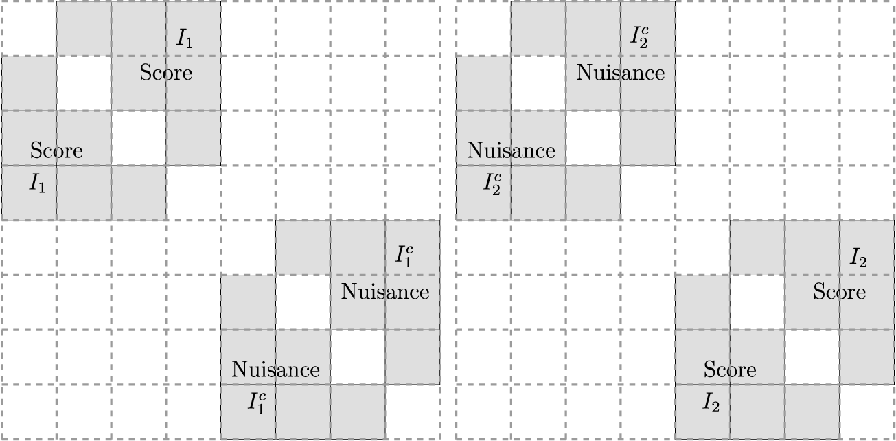

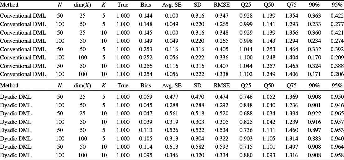
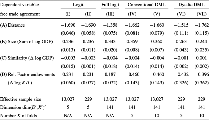


 Open access