








1 Introduction
Rational homotopy theory (RHT) studies homotopy theory “modulo torsion groups,” through localization with respect to the empty set of primes. This construction associates to every simply connected space X its rationalization, denoted
$X_{0}$
 , with the property that
$\pi _n(X)\otimes \mathbb {Q} \cong \pi _n(X_{0})$
, with the property that
$\pi _n(X)\otimes \mathbb {Q} \cong \pi _n(X_{0})$
 for any integer n. Two such spaces X and Y are said to be rationally homotopy equivalent, written
$X \sim _{\mathbb {Q}} Y$
for any integer n. Two such spaces X and Y are said to be rationally homotopy equivalent, written
$X \sim _{\mathbb {Q}} Y$
 , if their rationalizations
$X_{0}$
, if their rationalizations
$X_{0}$
 and
$Y_{0}$
and
$Y_{0}$
 are homotopy equivalent. Thus, RHT is the study of spaces up to rational homotopy equivalence, and X is said to be rational if the
$\mathbb {Z}$
are homotopy equivalent. Thus, RHT is the study of spaces up to rational homotopy equivalence, and X is said to be rational if the
$\mathbb {Z}$
 -module
$\pi _n(X)$
-module
$\pi _n(X)$
 (or equivalently,
$H_{n}(X, \mathbb {Z})$
(or equivalently,
$H_{n}(X, \mathbb {Z})$
 ) is a
$\mathbb {Q}$
) is a
$\mathbb {Q}$
 -vector space for each
$n\geq 1$
-vector space for each
$n\geq 1$
 . Ignoring torsion in homotopy and homology groups of X sacrifices many properties (e.g., those arising from Steenrod operations), but it yields a complete algebraic invariant of its rational equivalence class.
Within the theory, a fundamental result by Y. Félix and S. Halperin states that finite 1-connected CW-complexes and more generally spaces of finite Lusternik–Schnirelmann category cat(X) are naturally distributed into two distinct classes: the elliptic ones and the hyperbolic ones. The former are characterized by the fact that the ranks of their homotopy groups are almost all zero. Moreover, they all satisfy the Poincaré duality property over
$\mathbb {Q}$
 , and their Euler characteristics are nonnegative. Recall that X is said to be
Poincaré duality space over
$\mathbb {Q}$
, and their Euler characteristics are nonnegative. Recall that X is said to be
Poincaré duality space over
$\mathbb {Q}$
 if its graded rational cohomology algebra
$H^*(X,\mathbb {Q})$
if its graded rational cohomology algebra
$H^*(X,\mathbb {Q})$
 satisfies the Poincaré duality property (cf. §2 below). For instance, in Riemannian geometry, the simply connected Dupin hypersurfaces in
$\mathbb {S}^n$
satisfies the Poincaré duality property (cf. §2 below). For instance, in Riemannian geometry, the simply connected Dupin hypersurfaces in
$\mathbb {S}^n$
 are elliptic. Moreover, all known examples of simply connected positively curved manifolds are elliptic, and a conjecture of Bott asserts that they all should be [Reference Félix, Halperin and Thomas5, Reference Félix, Halperin and Thomas6].
Our work leverages Sullivan’s algebraic approach to RHT, specifically the Sullivan minimal model defined in §2. We will focus on spaces X having the homotopy type of simply connected finite-type CW-complexes. Each such space has a Sullivan minimal model, i.e., a free commutative differential graded algebra
$(\Lambda V,d)$
 , where V is a graded finite-type vector space, which is equipped with a decomposable differential
$d = d_k + d_{k+1} + \dots $
, where V is a graded finite-type vector space, which is equipped with a decomposable differential
$d = d_k + d_{k+1} + \dots $
 (
$k\geq 2$
(
$k\geq 2$
 ). This model satisfies
$H^*(X,\mathbb {Q})\cong H^*(\Lambda V,d)$
). This model satisfies
$H^*(X,\mathbb {Q})\cong H^*(\Lambda V,d)$
 and
$V \cong \mathrm{Hom}_{\mathbb {Z}}(\pi _*(X),\mathbb {Q})$
and
$V \cong \mathrm{Hom}_{\mathbb {Z}}(\pi _*(X),\mathbb {Q})$
 [Reference Sullivan20]. In this context, X is (rationally) elliptic if and only if V and
$H^*(\Lambda V,d)$
[Reference Sullivan20]. In this context, X is (rationally) elliptic if and only if V and
$H^*(\Lambda V,d)$
 are both finite dimensional. Each elliptic space satisfies the Poincaré duality property, hence, it is specified among other invariant, by its fundamental class, denoted
$\omega $
are both finite dimensional. Each elliptic space satisfies the Poincaré duality property, hence, it is specified among other invariant, by its fundamental class, denoted
$\omega $
 . The degree of
$\omega $
. The degree of
$\omega $
 , the maximal one, is called the formal dimension of X. If only
$\dim V$
, the maximal one, is called the formal dimension of X. If only
$\dim V$
 is finite, referring to [Reference Murillo17], X is in a larger class than that of Poincaré spaces, namely, the class of Gorenstein spaces (cf. §2 below for more details). One of the main ingredients we will use is the Milnor–Moore spectral sequence (2.9) (see §2). This provides an algebraic definition of a good lower bound of the rational LS-category
$\mathrm{cat}_0(X):=\mathrm{cat}(X_0)$
is finite, referring to [Reference Murillo17], X is in a larger class than that of Poincaré spaces, namely, the class of Gorenstein spaces (cf. §2 below for more details). One of the main ingredients we will use is the Milnor–Moore spectral sequence (2.9) (see §2). This provides an algebraic definition of a good lower bound of the rational LS-category
$\mathrm{cat}_0(X):=\mathrm{cat}(X_0)$
 , namely, the rational Toomer invariant
$e_0(X)$
, namely, the rational Toomer invariant
$e_0(X)$
 as follows:

with
$E_{\infty }^{m,*}(\Lambda V)$
 , the infinity term of (2.9). Referring to [Reference Félix, Halperin and Lemaire3],
$cat_0(X)=e_0(X)$
, the infinity term of (2.9). Referring to [Reference Félix, Halperin and Lemaire3],
$cat_0(X)=e_0(X)$
 for every elliptic space X.
Focusing on the differential, clearly its lower (homogeneous part)
$d_k$
 is also a differential so that
$(\Lambda V,d_k)$
is also a differential so that
$(\Lambda V,d_k)$
 is also a commutative differential graded algebra (cdga for short). If
$(\Lambda V,d_k)$
is also a commutative differential graded algebra (cdga for short). If
$(\Lambda V,d_k)$
 is elliptic, by the convergence of (2.9), so is
$(\Lambda V,d)$
is elliptic, by the convergence of (2.9), so is
$(\Lambda V,d)$
 . Moreover, in such a case, we have [Reference Lechuga and Murillo13, Proposition 3]

The main goal of this work is to give an explicit algorithm to determine
$e_0(\Lambda V,d)$
 when
$(\Lambda V,d_k)$
when
$(\Lambda V,d_k)$
 is not necessarily elliptic, hence an exact value of
$\mathrm{cat}_0(X)$
is not necessarily elliptic, hence an exact value of
$\mathrm{cat}_0(X)$
 for every arbitrary rationally elliptic space X.
Thereafter,
$\dim V$
 is finite and, while
$(\Lambda V,d_k)$
is finite and, while
$(\Lambda V,d_k)$
 is not necessarily elliptic, we still suppose that
$(\Lambda V,d)$
is not necessarily elliptic, we still suppose that
$(\Lambda V,d)$
 is elliptic. Hence, referring to [Reference Murillo17], we know that
$(\Lambda V,d_k)$
is elliptic. Hence, referring to [Reference Murillo17], we know that
$(\Lambda V,d_k)$
 and
$(\Lambda V,d)$
and
$(\Lambda V,d)$
 are Gorenstein algebras with the same formal dimension
${N=\max \{r\; | H^r(\Lambda V,d_k)\neq 0\}}$
are Gorenstein algebras with the same formal dimension
${N=\max \{r\; | H^r(\Lambda V,d_k)\neq 0\}}$
 . To treat this large class, we make use of the convergence Eilenberg–Moore spectral sequence (2.11) (see below). This was firstly introduced in [Reference Murillo17] and subsequently used in [Reference Rami19] to introduce, in the same spirit of
$e_0(X)$
. To treat this large class, we make use of the convergence Eilenberg–Moore spectral sequence (2.11) (see below). This was firstly introduced in [Reference Murillo17] and subsequently used in [Reference Rami19] to introduce, in the same spirit of
$e_0(X)$
 , a new lower bound for
$cat(X)$
, a new lower bound for
$cat(X)$
 which we denote
$\mathrm {R}_0(X)$
which we denote
$\mathrm {R}_0(X)$
 and will use considerably below.
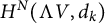
Using once more the hypothesis
$\dim V < \infty $
 , we see easily that
$H^N(\Lambda V,d_k)$
, we see easily that
$H^N(\Lambda V,d_k)$
 is finite dimensional. By a spectral sequence approach combined with an algorithm à la Lechuga–Murillo [Reference Lechuga and Murillo13], the third and fourth authors showed in [Reference Boutahir and Rami2] that one class
$\omega _0 \in H^N(\Lambda V,d_k)$
is finite dimensional. By a spectral sequence approach combined with an algorithm à la Lechuga–Murillo [Reference Lechuga and Murillo13], the third and fourth authors showed in [Reference Boutahir and Rami2] that one class
$\omega _0 \in H^N(\Lambda V,d_k)$
 survives to the infinity term of (2.9) and induces the fundamental class
$\omega $
survives to the infinity term of (2.9) and induces the fundamental class
$\omega $
 of
$(\Lambda V,d)$
of
$(\Lambda V,d)$
 . The Toomer invariant of
$(\Lambda V,d)$
. The Toomer invariant of
$(\Lambda V,d)$
 is then given explicitly by

Another cdga associated to
$(\Lambda V,d)$
 is the pure associated model,
$(\Lambda V,d_{\sigma })$
is the pure associated model,
$(\Lambda V,d_{\sigma })$
 [Reference Félix, Halperin and Thomas7, Reference Halperin9]. A spectacular result established by S. Halperin in [Reference Halperin9] states that
$(\Lambda V,d)$
[Reference Félix, Halperin and Thomas7, Reference Halperin9]. A spectacular result established by S. Halperin in [Reference Halperin9] states that
$(\Lambda V,d)$
 is elliptic if and only if
$(\Lambda V,d_{\sigma })$
is elliptic if and only if
$(\Lambda V,d_{\sigma })$
 is. When
$\dim V$
is. When
$\dim V$
 is finite,
$(\Lambda V,d_{\sigma })$
is finite,
$(\Lambda V,d_{\sigma })$
 is also a Gorenstein algebra with the same formal dimension as
$(\Lambda V,d)$
is also a Gorenstein algebra with the same formal dimension as
$(\Lambda V,d)$
 .
.
In §3, we give an algorithm to construct a generating class
$[f_{\sigma }]$
 of
$\mathrm{Ext}^N_{(\Lambda V,d_{\sigma })}(\mathbb {Q},(\Lambda V,d_{\sigma }))$
of
$\mathrm{Ext}^N_{(\Lambda V,d_{\sigma })}(\mathbb {Q},(\Lambda V,d_{\sigma }))$
 . In §4, by identifying the
$E_{\infty }$
. In §4, by identifying the
$E_{\infty }$
 term of the convergent spectral sequence (2.11) with
$\mathrm{Ext}^N_{(\Lambda V,d)}(\mathbb {Q},(\Lambda V,d))$
term of the convergent spectral sequence (2.11) with
$\mathrm{Ext}^N_{(\Lambda V,d)}(\mathbb {Q},(\Lambda V,d))$
 , we obtain, through an algorithm à la Lechuga–Murillo, a generating class
$[f_k^t]$
, we obtain, through an algorithm à la Lechuga–Murillo, a generating class
$[f_k^t]$
 of this latter from the generating class
$[f_k]$
of this latter from the generating class
$[f_k]$
 of
$\mathrm{Ext}^N_{(\Lambda V,d_k)}(\mathbb {Q},(\Lambda V,d_k))$
of
$\mathrm{Ext}^N_{(\Lambda V,d_k)}(\mathbb {Q},(\Lambda V,d_k))$
 . Finally, in §5, we use the spectral sequence (5.4) (see below), introduced in [Reference Rami18], to build a generating class
$[f_{\sigma }^l]$
. Finally, in §5, we use the spectral sequence (5.4) (see below), introduced in [Reference Rami18], to build a generating class
$[f_{\sigma }^l]$
 of
$\mathrm{Ext}^N_{(\Lambda V,d)}(\mathbb {Q},(\Lambda V,d))$
of
$\mathrm{Ext}^N_{(\Lambda V,d)}(\mathbb {Q},(\Lambda V,d))$
 from
$[f_{\sigma }]$
from
$[f_{\sigma }]$
 .
.
By way of a summary, given an elliptic space X with Sullivan minimal model
$(\Lambda V,d)$
 , by applying the algorithm in §3 to
$(\Lambda V,(d_{k})_{\sigma }),$
, by applying the algorithm in §3 to
$(\Lambda V,(d_{k})_{\sigma }),$
 we obtain the generating class, denoted
$[f_{k,\sigma }]$
we obtain the generating class, denoted
$[f_{k,\sigma }]$
 , of
$\mathrm{Ext}^{N}_{(\Lambda V,(d_{k})_{\sigma })}(\mathbb {K},(\Lambda V,(d_{k})_{\sigma }))$
, of
$\mathrm{Ext}^{N}_{(\Lambda V,(d_{k})_{\sigma })}(\mathbb {K},(\Lambda V,(d_{k})_{\sigma }))$
 . Then, noticing that
$(d_{k})_{\sigma }= (d_{\sigma })_{k}$
. Then, noticing that
$(d_{k})_{\sigma }= (d_{\sigma })_{k}$
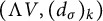
 , we apply the algorithm developed in §4 to
$(\Lambda V, (d_{\sigma })_{k})$
, we apply the algorithm developed in §4 to
$(\Lambda V, (d_{\sigma })_{k})$
 to get the generating class
$[f_{k,\sigma }^t]$
to get the generating class
$[f_{k,\sigma }^t]$
 of
$\mathrm{Ext}^{N}_{(\Lambda V,d_{\sigma })}(\mathbb {K},(\Lambda V,d_{\sigma }))$
of
$\mathrm{Ext}^{N}_{(\Lambda V,d_{\sigma })}(\mathbb {K},(\Lambda V,d_{\sigma }))$
 . We then use the algorithm described in §5 to
$(\Lambda V, d_{\sigma })$
. We then use the algorithm described in §5 to
$(\Lambda V, d_{\sigma })$
 to obtain the generating class
$[(f_{k,\sigma }^ t)^l]$
to obtain the generating class
$[(f_{k,\sigma }^ t)^l]$
 of
$\mathrm{Ext}^{N}_{(\Lambda V,d)}(\mathbb {K},(\Lambda V,d)$
of
$\mathrm{Ext}^{N}_{(\Lambda V,d)}(\mathbb {K},(\Lambda V,d)$
 .
.
As a summary, our algorithm complements those developed successively in [Reference Boutahir and Rami2, Reference Lechuga and Murillo13, Reference Murillo15]. Indeed, a combination of their contributions makes it possible to determine
$e_0$
 and therefore
$cat_0$
and therefore
$cat_0$
 in a quasi-complete way. The missing point is that this way does not allow us to know, when
$H^*(\Lambda V,d_{k, \sigma })$
in a quasi-complete way. The missing point is that this way does not allow us to know, when
$H^*(\Lambda V,d_{k, \sigma })$
 does not verify the Poincaré property, which of the generators of
$H^N(\Lambda V,d_{k, \sigma })$
does not verify the Poincaré property, which of the generators of
$H^N(\Lambda V,d_{k, \sigma })$
 persists up to the infinite level of the spectral sequence (2.9). Our work contributes to the extension of subsequent algorithms to the level of
$Ext$
persists up to the infinite level of the spectral sequence (2.9). Our work contributes to the extension of subsequent algorithms to the level of
$Ext$
 and thus takes advantage of the fact that
$(\Lambda V,d_{k, \sigma })$
and thus takes advantage of the fact that
$(\Lambda V,d_{k, \sigma })$
 is a Gorenstein algebra.
With the notations above, our main result reads as follows.
Theorem 1.1 Let X be a rationally elliptic space. Then, its fundamental class is given by
$[(f_{k,\sigma }^t)^l(1)]$
 . Hence,
$\mathrm{cat}_0(X) = e_0(X) = e_0([(f_{k,\sigma }^t)^l(1)]).$
. Hence,
$\mathrm{cat}_0(X) = e_0(X) = e_0([(f_{k,\sigma }^t)^l(1)]).$

Note that, in [Reference Lechuga10, Proposition 20], L. Lechuga constructed an algorithm to compute the rational category of any elliptic space under the condition
$(d - d_{\sigma })V \subseteq \Lambda ^{>l_{\sigma }}V$
 , where
$l_{\sigma }=l_0(\Lambda V,d_{\sigma })$
, where
$l_{\sigma }=l_0(\Lambda V,d_{\sigma })$
 . This algorithm is based on Gröebner basis calculus, which computes
$l_{\sigma }$
. This algorithm is based on Gröebner basis calculus, which computes
$l_{\sigma }$
 . Our result is therefore a generalization of Lechuga’s. Moreover, using the algorithm given in §4, we obtain an explicit formula for
$l_0(X)$
. Our result is therefore a generalization of Lechuga’s. Moreover, using the algorithm given in §4, we obtain an explicit formula for
$l_0(X)$
 as follows.
Theorem 1.2 (Theorem 4.3)
Let X be a rationally elliptic space. Then,
$l_0(X)=L_0(X) = t-1$
 .
.
This in particular gives a method to compute
$l_0(\Lambda V,d)$
 for any cdga
$(\Lambda V,d)$
for any cdga
$(\Lambda V,d)$
 which is in fact alternative and more general than the one given in [Reference Lechuga10]. Recall that
$L_0(X)$
which is in fact alternative and more general than the one given in [Reference Lechuga10]. Recall that
$L_0(X)$
 is the Ext-Ginsburg invariant introduced recently in [Reference Acharqy and Rami1] in the spirit of Ginsburg’s classical invariant
$l_0(X)$
is the Ext-Ginsburg invariant introduced recently in [Reference Acharqy and Rami1] in the spirit of Ginsburg’s classical invariant
$l_0(X)$
 .
.
Using this coincidence between
$l_0(X)$
 and
$L_0(X)$
and
$L_0(X)$
 , we give an alternative and explicit proof of [Reference Acharqy and Rami1, Theorem 1] which improves [Reference Rami19, Theorem 1] as follows.
Theorem 1.3 (Theorem 4.4)
Let X be a rationally elliptic space. Then,
$\mathrm {R}_0(X) = e_0(X) = cat_0(X)$
 .
.
We present the proofs of Theorems 1.2 and 1.3 in §4, while the proof of Theorem 1.1 is reported in §5. §6, entitled “Concluding remarks,” is devoted to some comments on our main result as well as its interaction with previous results on the subject.
2 Preliminaries
2.1 Frequently used notations
Throughout the article, we adopt the following consistent notation (all differentials are understood with respect to the appropriate cdga):
-
• $(\Lambda V, d)$
 : minimal Sullivan model of the space X, where V is the graded vector space of generators.
 -
• $d = \sum _{i\ge k} d_i$
: decomposition of the differential on
$(\Lambda V,d)$
with
$d_i(V)\subset \Lambda ^{i}V$
;
$d_k$
is the quadratic part (lowest homogeneous component). -
• $d_\sigma $
: the pure (associated) differential, satisfying
$d_\sigma (V^{\mathrm {even}})=0$
and
$d_\sigma (V^{\mathrm {odd}})\subset \Lambda V^{\mathrm {even}}$
. -
• $(\Lambda V, d_\sigma )$
: pure model associated with
$(\Lambda V, d)$
. -
• $(d_k)_\sigma = (d_\sigma )_k$
: the pure quadratic model. -
• $sV$
: suspension of V, with
$|sv| = |v|-1$
. -
• $(\Lambda V \otimes \Lambda sV, D)$
: semifree resolution of
$\mathbb {K}$
as a
$(\Lambda V,d)$
-module. -
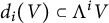
• $A = \mathrm{Hom}_{\Lambda V}(\Lambda V \otimes \Lambda sV, \Lambda V)$
: chain complex whose cohomology is the Ext-group. -
• D: total differential on A, defined by $D(f) = f\circ D_{\Lambda V\otimes \Lambda sV} + (-1)^{|f|+1} d_{\Lambda V}\circ f$
. -
• $D_k$
,
$D_\sigma $
: differentials on A induced by
$d_k$
and
$d_\sigma $
, respectively. -
• $\xi _i$
: successive corrections in the Lechuga–Murillo procedure (Eilenberg–Moore spectral sequence, §4). -
• $\beta _i$
: successive corrections in the odd-Eilenberg–Moore spectral sequence (§5). -
• $N = fd(\Lambda V, d)$
: formal dimension of the Gorenstein algebra. -
• $ev$
: evaluation map
$ev: \mathrm{Ext}_{(\Lambda V,d)}(\mathbb {K}, (\Lambda V,d)) \to H(\Lambda V,d)$
.





















We also use the standard bi-grading and filtration degrees in the spectral sequences (Milnor–Moore, Eilenberg–Moore, and odd variants), with p the filtration degree and q the complementary degree. Indices, such as
$h_0^0$
 ,
$h_1^1$
,
$h_1^1$
 ,
$E_k^{p,q}$
,
$E_k^{p,q}$
 , etc., are used consistently throughout the spectral sequence arguments.
2.2 Sullivan models
In this subsection, we assume
$\mathbb {K}$
 of characteristic zero. The standard reference for this section is [Reference Félix, Halperin and Thomas7].
Let
$V=\oplus _{i\geq 1}V^{i}$
 be a graded vector space over
$\mathbb {K}$
be a graded vector space over
$\mathbb {K}$
 . The free commutative graded algebra over V, denoted
$\Lambda V$
. The free commutative graded algebra over V, denoted
$\Lambda V$
 , is the quotient of the tensor graded algebra
$TV$
, is the quotient of the tensor graded algebra
$TV$
 by the graded ideal I generated by homogeneous elements of the form
$x\otimes y-(-1)^{| x | | y |}y\otimes x$
by the graded ideal I generated by homogeneous elements of the form
$x\otimes y-(-1)^{| x | | y |}y\otimes x$
 ;
$x, y \in V$
;
$x, y \in V$
 , where
$|z|$
, where
$|z|$
 denotes the degree of
$z\in V$
denotes the degree of
$z\in V$
 . Thus,
$\Lambda V=\mathrm{Exterior}(V^{\text {odd}})\otimes \,\mathrm{Sym}(V^{\text {even}})=\bigoplus _{i\geq 0}\Lambda ^{i} V$
. Thus,
$\Lambda V=\mathrm{Exterior}(V^{\text {odd}})\otimes \,\mathrm{Sym}(V^{\text {even}})=\bigoplus _{i\geq 0}\Lambda ^{i} V$
 with
$\Lambda ^{i} V$
with
$\Lambda ^{i} V$
 denoting the linear span of the elements
$v_{1}^{n_{1}}\ldots v_{r}^{n_{r}}$
denoting the linear span of the elements
$v_{1}^{n_{1}}\ldots v_{r}^{n_{r}}$
 ;
${n_{1}+\cdots +n_{r}=i}$
;
${n_{1}+\cdots +n_{r}=i}$
 and
$n_{i}=1$
and
$n_{i}=1$
 if
$v_{i}\in V^{\text {odd}}$
if
$v_{i}\in V^{\text {odd}}$
 .
.
A Sullivan algebra is a commutative cochain algebra
$(\Lambda V,d)$
 generated by the graded vector space
$V=\oplus _{i\geq 1}V^{i}$
generated by the graded vector space
$V=\oplus _{i\geq 1}V^{i}$
 that is the union of an increasing sequence of graded subspaces
$\{V(k)\}_{k\geq 0}$
that is the union of an increasing sequence of graded subspaces
$\{V(k)\}_{k\geq 0}$
 such that
$d=0$
such that
$d=0$
 on
$V(0)$
on
$V(0)$
 and
$d: V(k)\rightarrow \Lambda V(k-1),\; k\geq 1$
and
$d: V(k)\rightarrow \Lambda V(k-1),\; k\geq 1$
 . In other words, d preserves each
$\Lambda V(k)$
. In other words, d preserves each
$\Lambda V(k)$
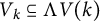
 and there exists a subspace
$V_k\subseteq \Lambda V(k)$
and there exists a subspace
$V_k\subseteq \Lambda V(k)$
 such that
$\Lambda V(k) = \Lambda V(k-1)\otimes V_k$
such that
$\Lambda V(k) = \Lambda V(k-1)\otimes V_k$
 and
$d: V_k\rightarrow \Lambda V(k-1),\; k\geq 1$
and
$d: V_k\rightarrow \Lambda V(k-1),\; k\geq 1$
 . Such an algebra is called minimal if moreover:

If
$(\Lambda V,d)$
 is
$1$
is
$1$
 -connected, that is,
$V^{1}=0$
-connected, that is,
$V^{1}=0$
 , then
$(\Lambda V,d)$
, then
$(\Lambda V,d)$
 is minimal if and only if

A Sullivan model for a cdga
$(A,d)$
 is a quasi-isomorphism (i.e., a morphism inducing an isomorphism in cohomology):

from a Sullivan algebra
$(\Lambda V ,d)$
 . Often we simply say that
$(\Lambda V,d)$
. Often we simply say that
$(\Lambda V,d)$
 is a model of
$(A,d)$
is a model of
$(A,d)$
 .
.
As shown in the foundational text by Félix, Halperin and Thomas [Reference Félix, Halperin and Thomas7, Proposition 12.2], any commutative cohomologically 1-connected cdga
$(A,d)$
 (i.e.,
$H^0(A)=\mathbb K$
(i.e.,
$H^0(A)=\mathbb K$
 and
$H^1(A)=0$
and
$H^1(A)=0$
 ) has a minimal Sullivan model.
If X is a path-connected topological space, a Sullivan model

of the cochains
$C^{*}(X,\mathbb {K})$
 on X is called a Sullivan model for X. In particular, if X is
$1$
on X is called a Sullivan model for X. In particular, if X is
$1$
 -connected, then it admits a minimal Sullivan model.
A KS-extension of an augmented cdga
$\epsilon :\, (A,d)\rightarrow (\mathbb {K},0)$
 (i.e., a cdga with the algebra morphism
$\epsilon $
(i.e., a cdga with the algebra morphism
$\epsilon $
 sending the ideal of augmentation
$A^+= A^{>0}$
sending the ideal of augmentation
$A^+= A^{>0}$
 to
$0$
to
$0$
 ) is an exact sequence of cdga morphisms

where
$d_{A\otimes \Lambda V}$
 restricts to
$d_A$
restricts to
$d_A$
 on A,
$dv_{i}\in A\otimes \Lambda V_{<i}$
on A,
$dv_{i}\in A\otimes \Lambda V_{<i}$
 , and
$(\Lambda V,\bar {d})$
, and
$(\Lambda V,\bar {d})$
 is a Sullivan algebra with differential
$\bar {d}$
is a Sullivan algebra with differential
$\bar {d}$
 denoting the obvious quotient differential induced by
$d_{A\otimes \Lambda V}$
denoting the obvious quotient differential induced by
$d_{A\otimes \Lambda V}$
 on V.
on V.
2.3 Differential Ext
In what follows, we fix
$(R,d)$
 as a cdga over
$\mathbb {K}$
as a cdga over
$\mathbb {K}$
 .
.
A left
$(R,d)$
 -module
$(M,d)$
-module
$(M,d)$
 is said to be semifree if M is the union of an increasing sequence
$\{M(k)\}_{k\geq 0}$
is said to be semifree if M is the union of an increasing sequence
$\{M(k)\}_{k\geq 0}$
 of
$(R,d)$
of
$(R,d)$
 -submodules such that
$M(0)$
-submodules such that
$M(0)$
 and each of the quotients
$M(k)/M(k-1)$
and each of the quotients
$M(k)/M(k-1)$
 are R-free modules on a basis of cycles. Such an increasing sequence is called a semifree filtration of
$(M,d)$
are R-free modules on a basis of cycles. Such an increasing sequence is called a semifree filtration of
$(M,d)$
 .
.
A semifree resolution of an
$(R,d)$
 -module
$(A,d)$
-module
$(A,d)$
 is an
$(R,d)$
is an
$(R,d)$
 -semifree module
$(M,d)$
-semifree module
$(M,d)$
 together with a quasi-isomorphism

of
$(R,d)$
 -modules. Recall from [Reference Félix, Halperin and Thomas7, Proposition 6.6] that:
-
(1) Every $(R,d)$
module
$(A,d)$
has a semifree resolution
$m:\, (M,d)\stackrel {\simeq }{\rightarrow }(A,d)$
. -
(2) If $m':\, (M',d)\stackrel {\simeq }{\rightarrow }(A,d)$
is a second semifree resolution, then there is an equivalence of
$(R,d)$
-modules
$\alpha : (M',d)\rightarrow (M,d)$
such that
$m \circ \alpha \sim m'$
.







Remark 2.1 Let
$\{M(k)\}$
 be a semifree filtration of
$(M,d)$
be a semifree filtration of
$(M,d)$
 . Then
$M(0)$
. Then
$M(0)$
 and each
$M(k)/M(k-1)$
and each
$M(k)/M(k-1)$
 have the form
$(R,d)\otimes (Z(k),0)$
have the form
$(R,d)\otimes (Z(k),0)$
 , where
$Z(k)$
, where
$Z(k)$
 is a free
$\mathbb {K}$
is a free
$\mathbb {K}$
 -module and so that each surjection
$M(k) \rightarrow R\otimes Z(k)$
-module and so that each surjection
$M(k) \rightarrow R\otimes Z(k)$
 splits as follows:

Thus, forgetting the differentials, we conclude that
$M=R\otimes (\bigoplus _{k=0}^{\infty })$
 is a free R-module.
Let
$\eta :\, (P,d)\rightarrow (Q,d)$
 be a morphism of
$(R,d)$
be a morphism of
$(R,d)$
 -modules, and for any third
$(R,d)$
-modules, and for any third
$(R,d)$
 -module
$(M,d)$
-module
$(M,d)$
 , denote by

the morphism of complexes induced by
$\eta $
 . Referring to [Reference Félix, Halperin and Thomas7, Proposition 6.4], if
$(M,d)$
. Referring to [Reference Félix, Halperin and Thomas7, Proposition 6.4], if
$(M,d)$
 is a semifree
$(R,d)$
is a semifree
$(R,d)$
 -module and
$\eta $
-module and
$\eta $
 is a quasi-isomorphism, then
-
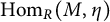
• $\mathrm{Hom}_{R}(M,\eta )$
is a quasi-isomorphism. -
• Given a diagram of morphism of $(R,d)$
-modules, (2.1) $$ \begin{align} \begin{array}{c c c} & & (P,d)\\ & & \downarrow \simeq \eta\\ (M,d) & \stackrel{\psi}{\rightarrow} & (Q,d) \end{array} \end{align} $$there is a unique homotopy class of morphisms $\phi :\,(M,d) \rightarrow (P,d)$
such that
$\eta \circ \phi \sim \psi $
.
-
• A quasi-isomorphism between semifree $(R,d)$
modules is an equivalence.

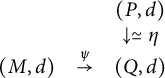



The second property is called the lifting lemma.
Given
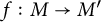
$f:\,M\rightarrow M'$
 and
$g:\,P'\rightarrow P,$
and
$g:\,P'\rightarrow P,$
 two R-linear morphisms between left
$(R,d)$
two R-linear morphisms between left
$(R,d)$
 -modules and
$h:\, Q\rightarrow Q'$
-modules and
$h:\, Q\rightarrow Q'$
 an R-linear morphism between right
$(R,d)$
an R-linear morphism between right
$(R,d)$
 -modules. We define

and

If moreover f, g, and h commute with the differentials, then
$\mathrm{Hom}_{R}(f,g)$
 and
$h\otimes _{R}f$
and
$h\otimes _{R}f$
 are morphisms of graded chain complexes. Furthermore, if
$(M,d)$
are morphisms of graded chain complexes. Furthermore, if
$(M,d)$
 and
$(M',d)$
and
$(M',d)$
 are
$(R,d)$
are
$(R,d)$
 -semifree, then [Reference Félix, Halperin and Thomas7, Proposition 6.7] the following holds:
-
(1) If f and g are quasi-isomorphisms, then so is $\mathrm{Hom}_{R}(f,g)$
. -
(2) If f and h are quasi-isomorphisms, then so is $h\otimes _{R}f$
.


Given two
$(A,d)$
 -modules
$(M,d)$
-modules
$(M,d)$
 and
$(N,d)$
and
$(N,d)$
 and
$(P,d)$
and
$(P,d)$
 a semifree resolution of
$(M,d)$
a semifree resolution of
$(M,d)$
 . The Eilenberg–Moore generalized functor called here the Ext differential is defined as follows:

It follows from the previous properties that this functor is independent of the choice of the semifree resolution of
$(M,d)$
 . More precisely,

where
$\mathrm{Hom}_{A}^{p,q}(P,N)=\mathrm{Hom}_{A}(P^{q},N^{p+q})$
 has the differential D defined for any
$f: P^q\rightarrow N^{p+q}$
has the differential D defined for any
$f: P^q\rightarrow N^{p+q}$
 , of degree p, by

So, we obtain the graduation:

where
$H^{p,j-p}(\mathrm{Hom}_{A}(P,N))$
 stands for the cohomology at the middle term in the following complex:

p is called the cohomological degree,
$q=j-p$
 the internal or the complementary degree, and j the total degree.
2.4 Gorenstein spaces and the evaluation map
In this subsection, we consider cohomologically
$1$
 -connected cdga’s and
$1$
-connected cdga’s and
$1$
 -connected spaces.
An augmented cdga
$(A,d)$
 is called a Gorenstein dga or simply a Gorenstein algebra if the graded
$\mathbb {K}$
is called a Gorenstein dga or simply a Gorenstein algebra if the graded
$\mathbb {K}$
 -vector space
$Ext_{A}(\mathbb {K},A)$
-vector space
$Ext_{A}(\mathbb {K},A)$
 is one-dimensional. The generating class
$\Omega $
is one-dimensional. The generating class
$\Omega $
 of
$\mathrm{Ext}_{A}(\mathbb {K},A)$
of
$\mathrm{Ext}_{A}(\mathbb {K},A)$
 and its degree
$|\Omega |$
and its degree
$|\Omega |$
 , denoted
$fd(A,d)$
, denoted
$fd(A,d)$
 , are called the fundamental class and formal dimension of
$(A,d), respectively$
, are called the fundamental class and formal dimension of
$(A,d), respectively$
 .
.
A pointed topological space X is said to be a Gorenstein space over
$\mathbb {K}$
 (with formal dimension denoted
$fd(X)$
(with formal dimension denoted
$fd(X)$
 ) if
$C^{*}(X,\mathbb {K})$
) if
$C^{*}(X,\mathbb {K})$
 is a Gorenstein algebra. Referring to [Reference Félix, Halperin and Thomas4], given a quasi-isomorphism
$A\stackrel {\simeq }{\rightarrow }B$
is a Gorenstein algebra. Referring to [Reference Félix, Halperin and Thomas4], given a quasi-isomorphism
$A\stackrel {\simeq }{\rightarrow }B$
 of augmented cdga’s, we obtain the following chain of isomorphisms:

This composition will be viewed as an identification, that is,

Thus, if
$(\Lambda V,d)$
 is a Sullivan model of
$(A,d)$
is a Sullivan model of
$(A,d)$
 (resp. of X), the latter is Gorenstein over
$\mathbb {K}$
(resp. of X), the latter is Gorenstein over
$\mathbb {K}$
 if and only if
$(\Lambda V,d)$
if and only if
$(\Lambda V,d)$
 is. This holds when V is finite dimensional [Reference Murillo17, Theorem A]. If, moreover,
$\dim H^{*}(\Lambda V,d)<\infty $
is. This holds when V is finite dimensional [Reference Murillo17, Theorem A]. If, moreover,
$\dim H^{*}(\Lambda V,d)<\infty $
 , then
$H^{*}(\Lambda V,d)$
, then
$H^{*}(\Lambda V,d)$
 satisfies Poincaré duality property over
$\mathbb {K}$
satisfies Poincaré duality property over
$\mathbb {K}$
 and
$fd(\Lambda V,d):=N$
and
$fd(\Lambda V,d):=N$
 is exactly the degree of its fundamental class
$[\omega ]$
is exactly the degree of its fundamental class
$[\omega ]$
 ; the unique generating element of
$H^N(\Lambda V, d)$
; the unique generating element of
$H^N(\Lambda V, d)$
 [Reference Murillo17, Theorem A]. Recall that a graded algebra A of finite dimension is called of formal dimension m if
$A^m\neq 0$
[Reference Murillo17, Theorem A]. Recall that a graded algebra A of finite dimension is called of formal dimension m if
$A^m\neq 0$
 and
$A^{>m} =0$
and
$A^{>m} =0$
 . Such an algebra is said a
Poincaré duality algebra or it satisfies
Poincaré duality property over
$\mathbb {K}$
. Such an algebra is said a
Poincaré duality algebra or it satisfies
Poincaré duality property over
$\mathbb {K}$
 if it is commutative and satisfies the following conditions:
-
(1) $A^m \cong \mathbb {K}\omega $
. -
(2) $\forall p, A^p\otimes A^{m-p} \rightarrow A^m \cong \mathbb {K}$
is a nondegenerate bilinear form.


The generating element
$\omega $
 of degree m is called the fundamental class of A.
Let
$(A,d)$
 be an augmented cdga and consider
$\mathbb {K}$
be an augmented cdga and consider
$\mathbb {K}$
 as a cdga with differential
$d_{\mathbb {K}}=0$
as a cdga with differential
$d_{\mathbb {K}}=0$
 . The chain evaluation map

induces in homology, the evaluation map [Reference Félix, Halperin and Thomas4, Reference Murillo16] is the linear map

Here,
$[f]$
 is a cohomology class represented by a cocycle
$f: (P,d) \rightarrow (A,d)$
is a cohomology class represented by a cocycle
$f: (P,d) \rightarrow (A,d)$
 , where
$(P,d)\stackrel {\simeq }{\rightarrow } (\mathbb {K},0)$
, where
$(P,d)\stackrel {\simeq }{\rightarrow } (\mathbb {K},0)$
 is an
$(A,d)$
is an
$(A,d)$
 -semifree resolution of
$\mathbb {K}$
-semifree resolution of
$\mathbb {K}$
 , and p is a cocycle in
$(P,d)$
, and p is a cocycle in
$(P,d)$
 representing
$1_{\mathbb {K}}$
representing
$1_{\mathbb {K}}$
 . Again, from (2.3), we deduce that
$ev_{A}$
. Again, from (2.3), we deduce that
$ev_{A}$
 is preserved by quasi-isomorphisms.
The evaluation map
$ev_{X}$
 of a pointed topological space X is by definition that of
$C^{*}(X;\mathbb {K})$
of a pointed topological space X is by definition that of
$C^{*}(X;\mathbb {K})$
 . Thus, if
$(\Lambda V,d)$
. Thus, if
$(\Lambda V,d)$
 is a minimal Sullivan model of X, we will make the following identification in what follows:

A result of Murillo [Reference Murillo16, Theorem A] states that when
$\dim V<\infty $
 ,
,

i.e., a Gorenstein algebra satisfies Poincaré duality if and only if its evaluation map is nonzero.
2.5 Spectral sequences
A cohomology spectral sequence (see [Reference Félix, Halperin and Thomas7, Reference McCleary14]) is a sequence of differential bi-graded complexes
$(E_{r}^{*,*},d_{r},\sigma _{r})$
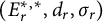 ,
$r\geq s$
,
$r\geq s$
 (some integer s) over
$\mathbb {K}$
(some integer s) over
$\mathbb {K}$
 with
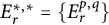
$E_{r}^{*,*}=\{E_{r}^{p,q}\}$
with
$E_{r}^{*,*}=\{E_{r}^{p,q}\}$
 ,
$d_{r}$
,
$d_{r}$
 is a differential of bi-degree
$(r,-r+1),$
is a differential of bi-degree
$(r,-r+1),$
 and
$\sigma _{r}:\, H(E_{r}^{*,*})\stackrel {\cong }{\rightarrow } E_{r+1}^{*,*}$
and
$\sigma _{r}:\, H(E_{r}^{*,*})\stackrel {\cong }{\rightarrow } E_{r+1}^{*,*}$
 is an isomorphism of bi-graded complexes.
The spectral sequence
$(E_{r},d_{r})$
 is called convergent if, for each
$(p,q),$
is called convergent if, for each
$(p,q),$
 there is an integer
$r(p,q)$
there is an integer
$r(p,q)$
 such that

In this case, the
$\infty $
 term of the spectral sequence is the bi-graded complex
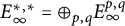
$E^{*,*}_{\infty } =\oplus _{p,q} E^{p,q}_{\infty }$
term of the spectral sequence is the bi-graded complex
$E^{*,*}_{\infty } =\oplus _{p,q} E^{p,q}_{\infty }$
 , where

Given a cdga
$(A,d)$
 . A filtration
$FA$
. A filtration
$FA$
 on
$(A,d)$
on
$(A,d)$
 is a family of graded subalgebras
$\{F^{p}A\}$
is a family of graded subalgebras
$\{F^{p}A\}$
 for
$p\in \mathbb {Z}$
for
$p\in \mathbb {Z}$
 so that

and
$d(F^{p}A) \subseteq F^{p}A$
 for all
$p\in \mathbb {Z}$
for all
$p\in \mathbb {Z}$
 . In particular, d induces a differential on each
$F^pA$
. In particular, d induces a differential on each
$F^pA$
 so that
$(F^pA,d_{F^pA})$
so that
$(F^pA,d_{F^pA})$
 becomes also a differential graded algebra. The filtered cdga
$(A, FA, d)$
becomes also a differential graded algebra. The filtered cdga
$(A, FA, d)$
 determines the associated differential bi-graded algebra
$(GA,Gd)$
determines the associated differential bi-graded algebra
$(GA,Gd)$
 , where

and
$Gd$
 is the differential naturally induced by d. Here, p is the filtration degree, q is the complementary degree, and
$p+q$
is the differential naturally induced by d. Here, p is the filtration degree, q is the complementary degree, and
$p+q$
 is the total degree.
Now, denote (for each integer
$r\geq 0$
 ) by
$Z_{r}^{p}$
) by
$Z_{r}^{p}$
 and
$B_{r}^{p}$
and
$B_{r}^{p}$
 the sub-algebras

and

Clearly,
$B_{0}^{p}\subset B_{1}^{p}\subseteq \dots B_{r}^{p}\subseteq \cdots \subseteq Z_{r}^{p}\subseteq \cdots \subseteq Z_{0}^{p}.$
 The r-term (
$r\geq 0$
The r-term (
$r\geq 0$
 ) of this spectral sequence is the bi-graded algebra
$E_{r}=\{E_{r}^{p,q}\}$
) of this spectral sequence is the bi-graded algebra
$E_{r}=\{E_{r}^{p,q}\}$
 , where

It follows from the definition that
$(E_{0},d_{0})=(GA,Gd)$
 and d factors to define a differential
$d_{r}$
and d factors to define a differential
$d_{r}$
 in
$E_{r}$
in
$E_{r}$
 of bi-degree
$(r,1-r)$
of bi-degree
$(r,1-r)$
 . Moreover, the inclusion
$Z_{r+1}^{p}\hookrightarrow Z_{r}^{p}$
. Moreover, the inclusion
$Z_{r+1}^{p}\hookrightarrow Z_{r}^{p}$
 induces an isomorphism of bi-graded algebras
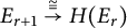
$E_{r+1}\stackrel {\cong }{\rightarrow } H(E_{r})$
induces an isomorphism of bi-graded algebras
$E_{r+1}\stackrel {\cong }{\rightarrow } H(E_{r})$
 and the filtration
$\{F^{p}A\}$
and the filtration
$\{F^{p}A\}$
 on A induces a filtration on
$H(A,d)$
on A induces a filtration on
$H(A,d)$
 as follows:

If the associated spectral sequence is convergent and there is an isomorphism
$E_{\infty }\cong GH(A)$
 of bi-graded algebras then, we say that it converges to
$H(A)$
of bi-graded algebras then, we say that it converges to
$H(A)$
 . This is expressed (quite often) by

2.5.1 Milnor–Moore and Eilenberg–Moore spectral sequences
In this section, we consider again cohomologically
$1$
 -connected cdga algebras
$1$
-connected cdga algebras
$1$
 -connected spaces.
Given a minimal Sullivan algebra
$(\Lambda V,d)$
 with
$d=d_{k}+d_{k+1}+\cdots $
with
$d=d_{k}+d_{k+1}+\cdots $
 (some
$k\geq 2$
(some
$k\geq 2$
 ), where
$d_{i}(V)\subset \Lambda ^{\geq i} V$
), where
$d_{i}(V)\subset \Lambda ^{\geq i} V$
 (
$\forall i\geq k$
(
$\forall i\geq k$
 ). Notice that
$d_k$
). Notice that
$d_k$
 is indeed a differential. We endow
$\Lambda V$
is indeed a differential. We endow
$\Lambda V$
 with the decreasing filtration:

It is straightforward to verify that
$(F^{p}\Lambda V)$
 is a decreasing sequence and
$dF^{p}\Lambda V \subset F^{p}\Lambda V$
is a decreasing sequence and
$dF^{p}\Lambda V \subset F^{p}\Lambda V$
 . Consequently, we obtain the so-called (convergent) Milnor–Moore spectral sequence:

Next (see [Reference Murillo17, Reference Rami19]), on the cdga
$A=(\mathrm{Hom}_{\Lambda V}((\Lambda V\otimes \Lambda sV,d),\Lambda V),D)$
 , where [Reference Félix, Halperin and Thomas7]
$(\Lambda V\otimes \Lambda sV,d)$
, where [Reference Félix, Halperin and Thomas7]
$(\Lambda V\otimes \Lambda sV,d)$
 stands for the
$(\Lambda V, d)$
stands for the
$(\Lambda V, d)$
 -semifree resolution of
$\mathbb {K}$
-semifree resolution of
$\mathbb {K}$
 with differential d extending that of
$\Lambda V$
with differential d extending that of
$\Lambda V$
 by
$dsv=v-sdv$
by
$dsv=v-sdv$
 , we consider the filtration

Notice that since f is a
$(\Lambda V, d)$
 -morphism, then,
$f\in F^pA$
-morphism, then,
$f\in F^pA$
 if and only if
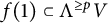
$f(\Lambda V \otimes \Lambda sV)\subset \Lambda ^{\geq p} V$
if and only if
$f(\Lambda V \otimes \Lambda sV)\subset \Lambda ^{\geq p} V$
 , that is,
$f(1)\subset \Lambda ^{\geq p} V$
, that is,
$f(1)\subset \Lambda ^{\geq p} V$
 and
$f(\Lambda sV)\subset \Lambda ^{\geq p} V$
and
$f(\Lambda sV)\subset \Lambda ^{\geq p} V$
 . Here again, it is straightforward to see that
$(F^{p}A)$
. Here again, it is straightforward to see that
$(F^{p}A)$
 is a decreasing sequence and
$dF^{p}A \subset F^{p}A$
is a decreasing sequence and
$dF^{p}A \subset F^{p}A$
 . Then, we get the Eilenberg–Moore spectral sequence [Reference Murillo17, Reference Rami19]:

Recall that a Sullivan algebra is called elliptic if
$\dim V$
 and
$\dim H(\Lambda V,d)$
and
$\dim H(\Lambda V,d)$
 are both finite dimensional. It results from the convergence of these spectral sequences that if
$(\Lambda V, d_{k})$
are both finite dimensional. It results from the convergence of these spectral sequences that if
$(\Lambda V, d_{k})$
 is an elliptic (resp. a Gorenstein) Sullivan algebra, then
$(\Lambda V, d)$
is an elliptic (resp. a Gorenstein) Sullivan algebra, then
$(\Lambda V, d)$
 is.
is.
2.5.2 Odd and odd-Eilenberg–Moore spectral sequences
To give a convenient characterization of ellipticity, S. Halperin associated [Reference Halperin9] to an arbitrary Sullivan algebra
$(\Lambda V,d)$
 whose generating space V is finite dimensional, another Sullivan algebra denoted
$(\Lambda V,d_{\sigma })$
whose generating space V is finite dimensional, another Sullivan algebra denoted
$(\Lambda V,d_{\sigma })$
 with differential
$d_{\sigma }$
with differential
$d_{\sigma }$
 satisfying:

$(\Lambda V,d_{\sigma })$
 is called the associated pure algebra of
$(\Lambda V,d)$
is called the associated pure algebra of
$(\Lambda V,d)$
 . Notice that the second property is equivalent to
$d_{\sigma }(V^{\text {odd}})\subseteq \Lambda V^{\text {even}}$
. Notice that the second property is equivalent to
$d_{\sigma }(V^{\text {odd}})\subseteq \Lambda V^{\text {even}}$
 . He then introduced the following spectral sequence:

which connects
$(\Lambda V,d)$
 and
$(\Lambda V,d_{\sigma })$
and
$(\Lambda V,d_{\sigma })$
 called the odd spectral sequence. Its main result states that
$\dim H(\Lambda V,d) < \infty \Leftrightarrow \dim H(\Lambda V,d_{\sigma }) < \infty .$
called the odd spectral sequence. Its main result states that
$\dim H(\Lambda V,d) < \infty \Leftrightarrow \dim H(\Lambda V,d_{\sigma }) < \infty .$
 Thus,
$(\Lambda V,d)$
Thus,
$(\Lambda V,d)$
 is elliptic if and only if
$(\Lambda V,d_{\sigma })$
is elliptic if and only if
$(\Lambda V,d_{\sigma })$
 is.
is.
Another spectral sequence, introduced by the fourth author in [Reference Rami18], is called the odd-Eilenberg–Moore or Ext-odd spectral sequence:

More details about it will be discussed in §5.
3 A basis of
$Ext_{(\Lambda V, d_{\sigma })}(\mathbb {K},(\Lambda V, d_{\sigma }))$

In this section, we construct a generating class of
$\mathrm{Ext}^N_{(\Lambda V, d_{\sigma })}(\mathbb {Q},(\Lambda V, d_{\sigma }))$
 for a pure Sullivan algebra. The algorithm proceeds in two steps:
-
(i) determination of f on $\Lambda V$
via the evaluation map, and -
(ii) recursive construction on $\Lambda sV$
by solving successive differential obstructions.


In this section, we assume
$\mathbb {K}=\mathbb {Q}$
 . Recall that a Sullivan algebra
$(\Lambda V,d)$
. Recall that a Sullivan algebra
$(\Lambda V,d)$
 is said to be pure if
$\dim V < \infty $
is said to be pure if
$\dim V < \infty $
 ,
$dV^{\text {even}}=0$
,
$dV^{\text {even}}=0$
 and
$dV^{\text {odd}}\subseteq \Lambda V^{\text {even}}$
and
$dV^{\text {odd}}\subseteq \Lambda V^{\text {even}}$
 [Reference Félix, Halperin and Thomas7, Reference Halperin9]. If moreover
$\dim H(\Lambda V, d)<\infty ,$
[Reference Félix, Halperin and Thomas7, Reference Halperin9]. If moreover
$\dim H(\Lambda V, d)<\infty ,$
 we say that
$(\Lambda V, d)$
we say that
$(\Lambda V, d)$
 is an elliptic pure Sullivan algebra. Any space whose minimal model is a pure (elliptic) model is called a pure (elliptic) space.
We assume that
$(\Lambda V, d)$
 is a minimal pure Sullivan algebra, that is,
$\dim V < \infty $
is a minimal pure Sullivan algebra, that is,
$\dim V < \infty $
 and its differential d satisfies
$d= \sum _k d_{\geq k}$
and its differential d satisfies
$d= \sum _k d_{\geq k}$
 (for some fixed
$k\geq 2$
(for some fixed
$k\geq 2$
 ),
$dV^{\text {even}}=0$
),
$dV^{\text {even}}=0$
 and
$dV^{\text {odd}}\subseteq \Lambda V^{\text {even}}$
and
$dV^{\text {odd}}\subseteq \Lambda V^{\text {even}}$
 .
.
Let
$(x_{1},\ldots ,x_{n})$
 be a basis of
$V^{\text {even}}$
be a basis of
$V^{\text {even}}$
 and
$(y_{1}, \ldots ,y_{m})$
and
$(y_{1}, \ldots ,y_{m})$
 be a basis of
$V^{\text {odd}}$
be a basis of
$V^{\text {odd}}$
 . Thus,

with
$dx_{i}=0$
 for all
$1\leq i\leq n$
for all
$1\leq i\leq n$
 and
$dy_{j}\in \mathbb {Q}[x_{1}, \ldots ,x_{n}]$
and
$dy_{j}\in \mathbb {Q}[x_{1}, \ldots ,x_{n}]$
 for all
$1\leq j\leq m$
for all
$1\leq j\leq m$
 . Its formal dimension is given by the formula [Reference Félix, Halperin and Thomas4, Proposition 5.2]:

A
$(\Lambda V, d)$
 -semifree resolution of
$(\mathbb {Q},0)$
-semifree resolution of
$(\mathbb {Q},0)$
 , called an acyclic closure of
$(\Lambda V, d)$
, called an acyclic closure of
$(\Lambda V, d)$
 (see [Reference Félix, Halperin and Thomas7]), is quasi-isomorphic to the cdga
$(\Lambda V\otimes (\mathbb {K}\oplus sV), d)$
(see [Reference Félix, Halperin and Thomas7]), is quasi-isomorphic to the cdga
$(\Lambda V\otimes (\mathbb {K}\oplus sV), d)$
 with differential (denoted also d) extending that of
$(\Lambda V,d)$
with differential (denoted also d) extending that of
$(\Lambda V,d)$
 as follows:

Therefore, being
$\dim V < \infty $
 ,
$(\Lambda V, d)$
,
$(\Lambda V, d)$
 is a Gorenstein algebra so, there exists a unique generating class
$\Omega = [f]$
is a Gorenstein algebra so, there exists a unique generating class
$\Omega = [f]$
 of
$\mathrm{Ext}_{(\Lambda V, d)}(\mathbb {Q},(\Lambda V, d))$
of
$\mathrm{Ext}_{(\Lambda V, d)}(\mathbb {Q},(\Lambda V, d))$
 represented by a non-degenerate cocycle morphism
$f\in \mathrm{Hom}_{(\Lambda V,d)}((\Lambda V\otimes (\mathbb {K}\oplus sV), d) , (\Lambda V, d))$
represented by a non-degenerate cocycle morphism
$f\in \mathrm{Hom}_{(\Lambda V,d)}((\Lambda V\otimes (\mathbb {K}\oplus sV), d) , (\Lambda V, d))$
 . In particular, we have
$D(f) = d\circ f + (-1)^{|f|+1} f\circ d = 0$
. In particular, we have
$D(f) = d\circ f + (-1)^{|f|+1} f\circ d = 0$
 (cf. (2.2)), that is,

The main result of this section is
Proposition 3.1 Let
$(\Lambda V,d)$
 be a pure (not necessarily elliptic) algebra. With the notations above, a basis class
$[f]$
be a pure (not necessarily elliptic) algebra. With the notations above, a basis class
$[f]$
 of
$\mathrm{Ext}_{(\Lambda V, d)}(\mathbb {Q},(\Lambda V, d))$
of
$\mathrm{Ext}_{(\Lambda V, d)}(\mathbb {Q},(\Lambda V, d))$
 is completely determined by
$f(\omega )$
is completely determined by
$f(\omega )$
 and
$f(sx_{i})$
and
$f(sx_{i})$
 for all
$x_i$
for all
$x_i$
 in
$V^{\mathrm{even}}$
in
$V^{\mathrm{even}}$
 .
.
Proof 1 Conceptual step: Construction of the generating class
The algorithm determines the unique (up to scalar) cocycle f representing the generator of
$\mathrm{Ext}_{(\Lambda V, d_{\sigma })}^N(\mathbb {Q},(\Lambda V, d_{\sigma }))$
 in two conceptual steps: (i) fixing f on
$\Lambda V$
in two conceptual steps: (i) fixing f on
$\Lambda V$
 via the evaluation map and (ii) solving the differential obstructions recursively on
$\Lambda sV$
via the evaluation map and (ii) solving the differential obstructions recursively on
$\Lambda sV$
 .
.
Technical verification:
-
• We begin by considering the case, where $ev_{\Lambda V}\neq 0$
so that
$(\Lambda V,d)$
is elliptic [Reference Murillo16, Theorem A], hence, a Poincaré duality algebra with a nonzero fundamental class
$\omega $
. Since
$\Lambda V\otimes (\mathbb {K}\oplus sV)$
is positively graded, we may put
$p=1_{\mathbb {Q}}:=1$
so that
$\omega = ev_{(\Lambda V,d)}:= [f(1)]$
.Recall that an explicit expression of a cocycle representing $\omega $
is given, for instance, in [Reference Murillo15]. Then, since f is a
$(\Lambda V,d)$
-module, it remains to determine it on
$\Lambda sV$
. For this, since
$(\Lambda V, d)$
is pure, formulas (3.2) and (3.3) above applied to
$sV^{\text {even}}$
and
$sV^{\text {odd}}$
reduce, respectively, to: (3.4) $$ \begin{align} d(f(sx_{i}))= (-1)^{N}f(x_{i}) = (-1)^{N}x_i\omega \text{ and } d(f(sy_{j})) = (-1)^{N}y_{j}\omega -(-1)^{N}f(sdy_{j}). \end{align} $$
As $|x_i|\geq 2$
, we have
$|f(x_{i})|>N$
, so that
$d(f(x_{i}))= f(d(x_i))=0$
which implies that
$f(x_{i})=x_i\omega $
is a coboundary. Consequently, the first obstruction is to find
$T_{i}\in \Lambda V^{\text {even}}\otimes \Lambda ^+ V^{\text {odd}}$
for
$i=1, \ldots ,n$
satisfying
$dT_{i}=(-1)^{N}x_{i}\omega $
. We then put
$f(sx_{i})=T_{i}$
.For every cocycle $y_{j}$
, we determine
$S_j$
such that
$dS_{j}=(-1)^{N}y_{j}\omega $
. We then put
$f(sy_{j})=S_{j}$
.Now, for every $y_{j}$
which is not a cocycle, i.e.,
$dy_j\neq 0$
, let
$m_j$
denote the number of
$x_i's$
having degrees less than that of
$y_j$
. Noticing that
$dy_{j}\in \mathbb {Q}[x_{1},\ldots ,x_{n}]$
is decomposable, we should assume in the following sum: $$ \begin{align*}dy_{j}=\sum_{i_{1}\leq \cdots \leq i_{l_j}}\alpha_{i_{1} \ldots i_{l_j}}x_{i_{1}} \ldots x_{i_{l_j}};\; \alpha_{i_{1} \ldots i_{l_j}}\in \mathbb{Q}\end{align*} $$that $2\leq l_j\leq m_j$
. Here, by convention,
$\alpha _{i_{1} \ldots i_{l_j}}=0$
if
$|x_{i_{1}} \ldots x_{i_{l_j}}|\neq |y_j|+1$
. Hence, $$ \begin{align*}sdy_{j}=\sum_{i_{1}\leq \cdots \leq i_{l_j}}\alpha_{i_{1} \ldots i_{l_j}}x_{i_{1}} \ldots x_{i_{l_j-1}}sx_{i_{l_j}}.\end{align*} $$
It follows that
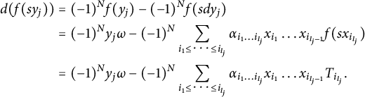
$$ \begin{align*} d(f(sy_{j})) &= (-1)^{N}f(y_{j})-(-1)^{N}f(sdy_{j}) \\ &= (-1)^{N}y_{j}\omega -(-1)^{N}\sum_{i_{1}\leq \cdots \leq i_{l_j}}\alpha_{i_{1} \ldots i_{l_j}}x_{i_{1}}\ldots x_{i_{l_j-1}}f(sx_{i_{l_j}}) \\ &= (-1)^{N}y_{j}\omega-(-1)^{N}\sum_{i_{1}\leq \cdots \leq i_{l_j}}\alpha_{i_{1} \ldots i_{l_j}}x_{i_{1}}\ldots x_{i_{l_j-1}}T_{i_{l_j}}. \end{align*} $$
Therefore, knowing $T_{i_{l_j}}$
, the second obstruction is to find
$S_{j}\in \Lambda V^{\text {even}}\otimes \Lambda ^+ V^{\text {odd}}$
satisfying the differential condition $$ \begin{align*}dS_{j}=(-1)^{N}y_{j}\omega-(-1)^{N}\sum_{i_{1}\leq \cdots \leq i_{l_j}}\alpha_{i_{1} \ldots i_{l_j}}x_{i_{1}}\ldots x_{i_{l_j-1}}T_{i_{l_j}}. \end{align*} $$
Notice that $x_{i_{l_j}}$
can reappear from
$T_{i_{l_j}}$
. We then put
$f(sy_{j})=S_{j}$
. -
• In the second case, $ev_{\Lambda V}=0$
. Then, by [Reference Lechuga and Murillo12, Corollary 3] (which characterizes the top class of a non-elliptic pure algebra), the top class
$\omega $
is a coboundary. Let us put
$\omega = d\omega '$
with
$|\omega '|=N-1$
. It is then straightforward to see that the above discussion applies with minor changes.Indeed, since for every $1 \leq i \leq n$
,
$dT_i = x_i\omega =dx_i\omega '$
, we may put
$T_i = x_i\omega '$
. Therefore, in this case,
$x_{i_{l_j}}$
reappears effectively from
$T_{i_{l_j}}$
and we have $$ \begin{align*}d[f(sy_{j}) - (-1)^{N}y_j\omega'] = [-(-1)^{N}\sum_{i_{1}\leq \cdots \leq i_{l_j}}\alpha_{i_{1}\ldots i_{l_j}} {x}_{i_{l_1}} \ldots x_{i_{l_j}}]\omega'. \end{align*} $$
Thus, we must check for an $S^{\prime }_j\in \Lambda V^{\text {even}}\otimes \Lambda ^+ V^{\text {odd}}$
such that $$ \begin{align*}d(S^{\prime}_j) = [-(-1)^{N}\sum_{i_{1}\leq \cdots \leq i_{l_j}}\alpha_{i_{1} \ldots i_{l_j}}x_{i_{1}} \ldots x_{i_{l_j}})]\omega'.\end{align*} $$
We then put $f(sy_{j}) - (-1)^{N}y_j\omega ' = S^{\prime }_j$
which gives $$ \begin{align*}f(sy_{j}) = (-1)^{N}y_j\omega' + S^{\prime}_j.\end{align*} $$







































Thus, we have constructed a generating class
$[f]$
 of
$\mathrm{Ext}_{(\Lambda V, d_{\sigma })}^N(\mathbb {Q},(\Lambda V, d_{\sigma }))$
of
$\mathrm{Ext}_{(\Lambda V, d_{\sigma })}^N(\mathbb {Q},(\Lambda V, d_{\sigma }))$
 . This class will be transported in §4 and §5 to obtain the generator of
$\mathrm{Ext}_{(\Lambda V, d)}^N(\mathbb {Q},(\Lambda V, d))$
. This class will be transported in §4 and §5 to obtain the generator of
$\mathrm{Ext}_{(\Lambda V, d)}^N(\mathbb {Q},(\Lambda V, d))$
 , allowing us to compute
$e_0(\Lambda ,d)=e_0([f(1)])$
, allowing us to compute
$e_0(\Lambda ,d)=e_0([f(1)])$
 and therefore
$\mathrm{cat}_0(X)$
and therefore
$\mathrm{cat}_0(X)$
 .
.
We now apply this procedure for particular examples.
Example 3.1 Consider the Sullivan model
$(\Lambda x_{2},x_{4},y_{5},y_{7}, d)$
 ,
$dx_{2}=dx_{4}=0$
,
$dx_{2}=dx_{4}=0$
 ,
$dy_{5}=x_{2}^{3}-2x_{2}x_{4}$
,
$dy_{5}=x_{2}^{3}-2x_{2}x_{4}$
 ,
$dy_{7}=x_{4}^{2}-x_{2}^{2}x_{4}$
,
$dy_{7}=x_{4}^{2}-x_{2}^{2}x_{4}$
 . This is clearly a pure elliptic Sullivan algebra. It is elliptic with formal dimension
$N=8$
. This is clearly a pure elliptic Sullivan algebra. It is elliptic with formal dimension
$N=8$
 and the fundamental class
$\omega =[x_{2}^{2}x_{4}-2x_4^2]$
and the fundamental class
$\omega =[x_{2}^{2}x_{4}-2x_4^2]$
 . So, let
$f(1)=x_{2}^{2}x_{4}-2x_4^2$
. So, let
$f(1)=x_{2}^{2}x_{4}-2x_4^2$
 . Applying the above algorithm, we get
$f(sx_{2})=x_{4}y_{5}$
. Applying the above algorithm, we get
$f(sx_{2})=x_{4}y_{5}$
 ,
$f(sx_{4})=x_{2}x_{4}y_{5}+(x_{2}^{2}-2x_4)y_{7}$
,
$f(sx_{4})=x_{2}x_{4}y_{5}+(x_{2}^{2}-2x_4)y_{7}$
 ,
$f(sy_{5})=2y_5y_7$
,
$f(sy_{5})=2y_5y_7$
 , and
$f(sy_{7})=x_{2}y_{5}y_{7}$
, and
$f(sy_{7})=x_{2}y_{5}y_{7}$
 . This determines the desired representative f of the generating class
$\Omega $
. This determines the desired representative f of the generating class
$\Omega $
 of
$\mathrm{Ext}_{(\Lambda V, d_{\sigma })}(\mathbb {K},(\Lambda V, d_{\sigma }))$
of
$\mathrm{Ext}_{(\Lambda V, d_{\sigma })}(\mathbb {K},(\Lambda V, d_{\sigma }))$
 .
.
Example 3.2 Let
$(\Lambda x_{2},x_{4},y_{5},y_{7}, d)$
 ,
$dx_{2}=dx_{4}=0$
,
$dx_{2}=dx_{4}=0$
 ,
$dy_{5}=-2x_{2}x_{4}$
,
$dy_{5}=-2x_{2}x_{4}$
 , and
$dy_{7}=x_{4}^{2}$
, and
$dy_{7}=x_{4}^{2}$
 . The differential
$d=d_2$
. The differential
$d=d_2$
 is homogeneous of degree two and such model is called a coformal Sullivan model. It is the associated quadratic model of
$(\Lambda x_{2},x_{4},y_{5},y_{7}, d)$
is homogeneous of degree two and such model is called a coformal Sullivan model. It is the associated quadratic model of
$(\Lambda x_{2},x_{4},y_{5},y_{7}, d)$
 . It is pure but non-elliptic model, since
$[x_2]^t\neq 0$
. It is pure but non-elliptic model, since
$[x_2]^t\neq 0$
 for any
$t\geq 1$
for any
$t\geq 1$
 . The class
$\omega _0 = [2x_{4}^{2}]$
. The class
$\omega _0 = [2x_{4}^{2}]$
 (whose degree equals
$N=8$
(whose degree equals
$N=8$
 ), although it is zero, it remains of interest for the determination of a representing cocycle of, say
$\Omega _0$
), although it is zero, it remains of interest for the determination of a representing cocycle of, say
$\Omega _0$
 of
$\mathrm{Ext}_{(\Lambda V, d)}(\mathbb {Q},(\Lambda V, d))$
of
$\mathrm{Ext}_{(\Lambda V, d)}(\mathbb {Q},(\Lambda V, d))$
 .
$\omega _0$
.
$\omega _0$
 is called the top class of
$(\Lambda V,d)$
is called the top class of
$(\Lambda V,d)$
 [Reference Lechuga and Murillo12]. We put (formally)
$f(1)= 2x_{4}^{2}$
[Reference Lechuga and Murillo12]. We put (formally)
$f(1)= 2x_{4}^{2}$
 (as in the second case
$(ii)$
(as in the second case
$(ii)$
 of the proof above). This yields, respectively:
-
• $d(f(sx_{2}))=f(x_{2})=x_2f(1)=2x_2x_4^2=d_2(ax_4y_5+bx_2y_7)$
, with a and b such that
$-2a+b=2$
, that is,
$b=2a+2$
. Therefore,
$f(sx_2)=ax_4y_5+2(a+1)x_2y_7)$
, some
$a\in \mathbb {Q}$
. -
• $d(f(sx_{4}))=f(x_{4})=2x_4^2=d(2x_{4}y_{7})$
. Hence,
$f(sx_{4})=2x_{4}y_{7}$
. -
• $d(f(sy_{5}))=f(y_5)-f(sd(y_5))=2x_4^2y_5+2x_2f(sx_4)=2x_4^2y_5+ 4x_2x_4y_7=d(-2y_5y_7)$
. Hence,
$f(sy_{5})=-2y_{5}y_{7}$
. -
• $df(sy_{7})=f(y_7)-f(sd(y_7))=2x_4^2y_7-x_4f(sx_4)=2x_4^2y_7- 2x_4^2y_7=0.$
Hence,
$f(sy_{7})=0$
.











This determines
$\Omega _0=[f]$
 .
.
4 A basis of
$\mathrm{Ext}_{(\Lambda V,d)}(\mathbb {K},(\Lambda V,d))$
from that of
$\mathrm{Ext}_{(\Lambda V,d_{k})}(\mathbb {K},(\Lambda V,d_{k}))$


In this section, we transport generators through the Eilenberg–Moore spectral sequence from
$(\Lambda V,d_{k})$
 to
$(\Lambda V,d)$
to
$(\Lambda V,d)$
 . We identify the
$E_{\infty }$
. We identify the
$E_{\infty }$
 -term with
$\mathrm{Ext}_{(\Lambda V,d)}^N(\mathbb K,(\Lambda V,d))$
-term with
$\mathrm{Ext}_{(\Lambda V,d)}^N(\mathbb K,(\Lambda V,d))$
 , recall the filtration, and apply the Lechuga–Murillo procedure to obtain the corrected generating class
$[f_k^t]$
, recall the filtration, and apply the Lechuga–Murillo procedure to obtain the corrected generating class
$[f_k^t]$
 . This yields the explicit computation of the Ginsburg invariant
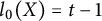
$l_0(X)=t-1$
. This yields the explicit computation of the Ginsburg invariant
$l_0(X)=t-1$
 .
.
We work with a minimal Sullivan algebra
$(\Lambda V,d)$
 , where

for a fixed
$k\geq 2$
 . We assume
$\dim V<\infty $
. We assume
$\dim V<\infty $
 and that
$(\Lambda V,d)$
and that
$(\Lambda V,d)$
 is elliptic, while
$(\Lambda V,d_k)$
is elliptic, while
$(\Lambda V,d_k)$
 need not be. Both algebras are then Gorenstein and share the same dimension N (see (3.1)).
As recalled in §2, they are linked by the Eilenberg–Moore spectral sequence (2.11). This sequence arises from the filtration

where
$A=\mathrm{Hom}_{\Lambda V}(\Lambda V\otimes \Lambda sV,\Lambda V)$
 . The differential on A is

We write
$d_{\Lambda V}$
 simply as d, and denote both
$D_A$
simply as d, and denote both
$D_A$
 and
$D_{\Lambda V\otimes \Lambda sV}$
and
$D_{\Lambda V\otimes \Lambda sV}$
 by D.
by D.
Degree reasons ensure that
$d_k$
 induces a differential
$D_k$
induces a differential
$D_k$
 on A. The first term of the spectral sequence is then

where p is the filtration degree and q its complement (so
$p+q$
 is the total degree).
Conceptual step: Transport via Eilenberg–Moore spectral sequence
We identify the
$E_{\infty }$
 -term of the convergent Eilenberg–Moore spectral sequence with
$\mathrm{Ext}_{(\Lambda V,d)}^N(\mathbb K,(\Lambda V,d))$
-term of the convergent Eilenberg–Moore spectral sequence with
$\mathrm{Ext}_{(\Lambda V,d)}^N(\mathbb K,(\Lambda V,d))$
 . The Lechuga–Murillo procedure then corrects the generator
$[f_k]$
. The Lechuga–Murillo procedure then corrects the generator
$[f_k]$
 of the quadratic level step by step.
Technical verification:
The Gorenstein property of
$(\Lambda V,d_k)$
 implies a unique bi-degree
$(p,q)$
implies a unique bi-degree
$(p,q)$
 with
$p+q=N$
with
$p+q=N$
 such that
$\operatorname {Ext}_{(\Lambda V,d_k)}(\mathbb {K},(\Lambda V,d_k))$
such that
$\operatorname {Ext}_{(\Lambda V,d_k)}(\mathbb {K},(\Lambda V,d_k))$
 is one-dimensional. Let
$[f]$
is one-dimensional. Let
$[f]$
 be its generator.
The Gorenstein property of
$(\Lambda V,d_{k})$
 implies a unique bi-degree
$(p,q)$
implies a unique bi-degree
$(p,q)$
 with
${p+q=N}$
with
${p+q=N}$
 such that
$\mathrm{Ext}_{(\Lambda V,d_{k})}(\mathbb {K},(\Lambda V,d_{k}))$
such that
$\mathrm{Ext}_{(\Lambda V,d_{k})}(\mathbb {K},(\Lambda V,d_{k}))$
 is one-dimensional. Let
$[f]$
is one-dimensional. Let
$[f]$
 be its generator. Using notation of §2, we have
$f\in Z^{p,q}_{k-1}$
be its generator. Using notation of §2, we have
$f\in Z^{p,q}_{k-1}$
 is the unique cocycle, up to a coboundary. Thus,

-
(1) Suppose that $Df=0$
.If moreover $f=Dg$
, for some
$g\in A^{N-1}$
, then
$f=D_{k}g+\sum _{i\geq k+1}D_{i}g$
. So,
$f-D_{k}g$
is a
$D_k$
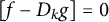
cocycle such that
$(f-D_{k}g)(\Lambda sV)\subset \Lambda ^{\geq p+1}V$
. Necessarily,
$[f-D_{k}g]=0$
in A. Otherwise, it should be a generating class of
$\mathrm{Ext}_{(\Lambda V,d_{k})}(\mathbb {K},(\Lambda V,d_{k}))$
. But, being of bi-degree
$(p+1, q-1)$
, we get a contradiction to the uniqueness of
$(p,q)$
. As a consequence, f is not a coboundary and its class is the desired generator (in this case) of A or equivalently, the spectral sequence (2.11) degenerates at the first term
$E_{k}$
.The same reasoning will be applied in the spectral sequence of §5, with the differential $d_k$
replaced by
$d_{\sigma }$
. -
(2) Assume that $Df\neq 0$
. Since
$Df$
is a
$(\Lambda V,d)$
-morphism, it is determined by its restriction to
$\Lambda sV$
. Let
$h^{0}_{i}$
denote the component mapping
$(\Lambda V\otimes \Lambda sV)^{r,s}$
to
$(\Lambda V)^{p+N+s+r+i+1,*}$
. For degree reasons, there exists a fixed integer
$t\geq 0$
such that $$ \begin{align*}Df_{|sV}=h^{0}_{0}+\cdots+h^{0}_{t}\end{align*} $$(with $h^0_t\neq 0$
). Indeed, if
$r= max\{|v_i|,\; v_i\in V\}$
, then [Reference Félix, Halperin and Thomas7, Corollary 1, p. 441] gives
$r\leq 2N-1$
and one obtains
$t\leq {(N+2-2p-2k+r)}/{2}$
.
This is equivalent to
(4.2) $$ \begin{align} Df(\Lambda sV)\subseteq \Lambda^{p+k-1}V\oplus\cdots\oplus\Lambda^{p+k-1+t}V. \end{align} $$
Until the last of section, we consider only the restrictions to $\Lambda sV$
.Now, since $D^{2}f=Dh^{0}_{0}+\cdots +Dh^{0}_{t}=0$
and, by word-length argument,
$D_{k}h^{0}_{0}=0$
(in fact,
$D_{k}h^{0}_{0}(\Lambda sV)\subset \Lambda ^{2(k-1)+p}V$
is the unique term which has this least word-length). But,
$|h^{0}_{0}|=N+1>N$
implies that there exist some
$\xi _{1}\in \mathrm{Hom}_{\Lambda V}(\Lambda V\otimes \Lambda sV;\Lambda V)$
such that
$h^{0}_{0}=D_{k}\xi _{1}$
. Moreover, as
$h^{0}_{0}(\Lambda sV)=D_{k}\xi _{1}(\Lambda sV)\subset \Lambda ^{p+k-1}V$
, we see that
$\xi _{1}(\Lambda sV)\subset \Lambda ^{p}V$
with total degree
$N={p+q}$
.We now introduce $f^{1}=f-\xi _{1}$
.On one hand, since, $Df^{1} = Df - D\xi _1 = h^{0}_{0}+\cdots +h^{0}_{t} - D_k\xi _1 - (D-D_{k})\xi _1 = (h^{0}_{1}- D_{k+1}\xi _1) + h^{0}_{2} + \cdots + h^{0}_{t} - D_{\geq k+2}\xi _1$
and
$D^2f^1 = 0$
, we have, for degree reason,
$D_k(h^{0}_{1}- D_{k+1}\xi _1) =0$
. So, being
$|h^{0}_{1}- D_{k+1}\xi _1| = N+1$
, there is some
$\xi _2\in A^{N}$
such that
$h^{0}_{1}- D_{k+1}\xi _1 = D_k\xi _2$
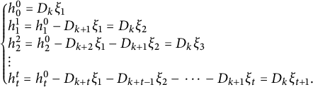
. This can be resumed (for the same t due again for analogous degree reason) as: $$ \begin{align*}Df^{1} = h_1^1 + h^{1}_{2}+\cdots+ h^{1}_{t},\end{align*} $$where $h_1^1 = h^{0}_{1}- D_{k+1}\xi _1 = D_k\xi _2$
.
We continue by introducing $f^2 =f^1 - \xi _2 = f - \xi _1 - \xi _2$
and repeat the process until we reach $$ \begin{align*}\left\{ \begin{array}{@{}l} f^t = f^{t-1} - \xi_t = f -\xi_1 - \cdots - \xi_t\\ Df^t=h_t^t = h_t^0 - D_{k+t}\xi_1 - D_{k+t-1}\xi_2 - \cdots - D_{k+1}\xi_t. \end{array} \right. \end{align*} $$
If $Df^t \neq 0$
, we continue the above process to get
$Df^t =h_t^t = D_k\xi _{t+1}$
(some
${\xi _{t+1}\in A^N}$
). But, by definition of
$t,$
we have
$D_{\geq k+1}(\xi _{t+1})=0$
. Therefore,
$Df^t = D\xi _{t+1}$
so that
$D(f^t -\xi _{t+1})=0$
. We (should) then take
$f^t -\xi _{t+1}$
instead of
$f^t$
.Then, to simplify, we assume that $Df^t= 0$
and show that
$f^t$
is not a coboundary.Assume that $f^t =Dg$
(some
$g\in A^{N-1})$
. On one hand, since all terms of the spectral sequence (2.11) are one-dimensional (as graded vector spaces), we still have $$ \begin{align*}f^t(\Lambda sV)\subseteq \Lambda^{p}V\oplus \cdots \oplus \Lambda^{p+t}V.\end{align*} $$
Thus, we should have $g(\Lambda sV)\subseteq \Lambda ^{p-k+1}V \oplus \cdots \oplus \Lambda ^{p+t-k+1}V$
so that $$ \begin{align*}g =g^0_0 + g_1^0 + \cdots + g_t^0,\end{align*} $$where $g_i^0(\Lambda (sV)\subseteq \Lambda ^{p-k+1+i}V$
. On the other hand, by (4.2), we should have $$ \begin{align*}f(\Lambda sV)\subseteq \Lambda^{p}V\oplus\cdots\oplus\Lambda^{p+t}V.\end{align*} $$
Thus, we may decompose f as
$$ \begin{align*}f =f^0_0 + f_1^0 + \cdots + f_t^0,\end{align*} $$where $f_i^0(\Lambda (sV))\subseteq \Lambda ^{p+i}V$
. It follows, using word-length argument, that
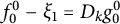
$f_0^0 - \xi _1 = D_kg^0_0$
, Hence,
$D_kf_0^0 - D_k\xi _1 = D_k^2(g_0^0)=0$
and since
$D_kf_0^0=0$
(by word length), we get
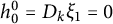
$h_0^0 =D_k\xi _1= 0$
. This contradicts the fact that
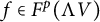
$f\in F^p(\Lambda V)$
. As a conclusion,
$[f^{t}]$
is a generating class of
$Ext^*_{(\Lambda V,d)}(\mathbb {K},(\Lambda V,d))$
.



























































Thus, the corrected generating class
$[f_k^t]$
 of
$\mathrm{Ext}_{(\Lambda V,d)}^N(\mathbb {K},(\Lambda V,d))$
of
$\mathrm{Ext}_{(\Lambda V,d)}^N(\mathbb {K},(\Lambda V,d))$
 has been obtained. By Theorem 1.2, this immediately gives the Ginsburg invariant
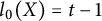
$l_0(X)=t-1$
has been obtained. By Theorem 1.2, this immediately gives the Ginsburg invariant
$l_0(X)=t-1$
 , and by Theorem 1.3, we have
$\mathrm {R}_0(X)=e_0(X)=\mathrm{cat}_0(X)$
, and by Theorem 1.3, we have
$\mathrm {R}_0(X)=e_0(X)=\mathrm{cat}_0(X)$
 .
.
Thus, we have established the following
Theorem 4.1 With the above notation, either the spectral sequence (2.11) degenerate at
$E_k$
 and
$[f]$
and
$[f]$
 generates
$\mathrm{Ext}^*_{(\Lambda V,d)}(\mathbb {K},(\Lambda V,d))$
generates
$\mathrm{Ext}^*_{(\Lambda V,d)}(\mathbb {K},(\Lambda V,d))$
 or else,
$[f^t]$
or else,
$[f^t]$
 is the generating class of
$\mathrm{Ext}^*_{(\Lambda V,d)}(\mathbb {K},(\Lambda V,d))$
is the generating class of
$\mathrm{Ext}^*_{(\Lambda V,d)}(\mathbb {K},(\Lambda V,d))$
 .
.
Remark 4.2 From the algorithm inducing
$f^t$
 , the following formulas arise:
We now describe how this is used explicitly to determine
$f^t$
 (cf. Example 4.2 below).
From the equation
$Df(1) = d(f(1)) = h_0^0(1) + h_1^0(1) + \cdots h_t^0(1)$
 with
$f(1)$
with
$f(1)$
 represents the generating class
$\omega _{0}$
represents the generating class
$\omega _{0}$
 of
$H(\Lambda V,d_k)$
of
$H(\Lambda V,d_k)$
 , we deduce the components
$h^0_i(1)$
, we deduce the components
$h^0_i(1)$
 (
$0\leq i\leq t$
(
$0\leq i\leq t$
 ). These are essential in obtaining iteratively the
$f^i$
). These are essential in obtaining iteratively the
$f^i$
 ’s (
$1\leq i\leq t$
’s (
$1\leq i\leq t$
 ) as follows: we first determine
$\xi _{1}(1)$
) as follows: we first determine
$\xi _{1}(1)$
 from the first equation, evaluated at
$1\in \mathbb {Q}$
from the first equation, evaluated at
$1\in \mathbb {Q}$
 . This determines
$\xi _{1}$
. This determines
$\xi _{1}$
 on
$\Lambda V$
on
$\Lambda V$
 . Then, we determine
$\xi _{1}$
. Then, we determine
$\xi _{1}$
 on
$\Lambda sV$
on
$\Lambda sV$
 and therefore,
$f^1 = f - \xi _{1}$
and therefore,
$f^1 = f - \xi _{1}$
 on
$\Lambda V \otimes \Lambda sV$
on
$\Lambda V \otimes \Lambda sV$
 . We proceed inductively using the
$(i+1)$
. We proceed inductively using the
$(i+1)$
 -th equation to determine
$\xi _{i}$
-th equation to determine
$\xi _{i}$
 , hence
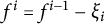
$f^i = f^{i-1}-\xi _i$
, hence
$f^i = f^{i-1}-\xi _i$
 on all
$\Lambda V \otimes \Lambda sV$
on all
$\Lambda V \otimes \Lambda sV$
 . As it is shown previously, the process terminates while we reach
$f^t$
. As it is shown previously, the process terminates while we reach
$f^t$
 .
.
Alternatively, we can apply the algorithm of Lechuga and Murillo [Reference Lechuga and Murillo13, Theorem 5] (or its extension [Reference Boutahir and Rami2]) to determine the
$\xi _{i}(1)$
 ; the only difference is that the first term is
$h_0^0(1)$
; the only difference is that the first term is
$h_0^0(1)$
 instead of
$h_1^0(1)$
instead of
$h_1^0(1)$
 .
.
Consequently, from
$f^t = f - \xi _1 - \xi _{2} - \cdots - \xi _t$
 , we obtain
$f^t(1) = f(1) - \xi _1(1) - \xi _{2}(1) - \cdots - \xi _t(1),$
, we obtain
$f^t(1) = f(1) - \xi _1(1) - \xi _{2}(1) - \cdots - \xi _t(1),$
 which indeed yields the fundamental class
$[f^t(1)] = ev_{(\Lambda V,d)}([f^t])$
which indeed yields the fundamental class
$[f^t(1)] = ev_{(\Lambda V,d)}([f^t])$
 of
$(\Lambda V,d)$
of
$(\Lambda V,d)$
 , that is, the generating class of
$H^N(\Lambda V,d)$
, that is, the generating class of
$H^N(\Lambda V,d)$
 .
.
4.1 Ext-Ginsburg and
$\mathrm {R}_0(\Lambda V,d)$
invariants

4.1.1 Ext-Ginsburg invariant
Recall that M. Ginsburg defined [Reference Ginsburg8], in terms of the following topological Milnor–Moore spectral sequence:

a homotopy invariant, denoted
$l_0(X)$
 , to be the largest integer j such that the differential
$d_j$
, to be the largest integer j such that the differential
$d_j$
 of the j-th term
$E_j$
of the j-th term
$E_j$
 is non-zero. He then showed that
$l_0(X) \leq \mathrm{cat}_0(X)$
is non-zero. He then showed that
$l_0(X) \leq \mathrm{cat}_0(X)$
 . For our purpose, we use the algebraic isomorphic spectral sequence (2.9) to give the following equivalent definition of
$l_0(X)$
. For our purpose, we use the algebraic isomorphic spectral sequence (2.9) to give the following equivalent definition of
$l_0(X)$
 :
:

or equivalently:

In other words,
$l_0(\Lambda V,d)+1$
 designates the stage where the spectral sequence (2.9) degenerate.
Notice that the two definitions agree, since, the first terms from
$E_2$
 up to
$E_{k-2}$
up to
$E_{k-2}$
 in (2.9) are all identical to the terms
$E_0 = (\Lambda V,0)$
in (2.9) are all identical to the terms
$E_0 = (\Lambda V,0)$
 and
$E_{k-1}\cong (\Lambda V,d_k)$
and
$E_{k-1}\cong (\Lambda V,d_k)$
 so that, if
$E_{\infty }^{p,q}=E_{s+1}^{p,q}$
so that, if
$E_{\infty }^{p,q}=E_{s+1}^{p,q}$
 in (4.3) and
$E_{\infty }^{p,q}(\Lambda V)=E_{t+1}^{p,q}(\Lambda V)$
in (4.3) and
$E_{\infty }^{p,q}(\Lambda V)=E_{t+1}^{p,q}(\Lambda V)$
 in (2.9) (where the first term is
$E_{k}^{p,q}(\Lambda V)$
in (2.9) (where the first term is
$E_{k}^{p,q}(\Lambda V)$
 ), then
$t+1$
), then
$t+1$
 should be equal to
$(s+1-k +1) +(k-1) =s+1$
should be equal to
$(s+1-k +1) +(k-1) =s+1$
 .
.
In the same spirit, we introduced [Reference Acharqy and Rami1] in terms of (2.11) an Ext-version of
$l_0(\Lambda V,d)$
 as follows:

(see (4.5) below for the definition of
$\delta _j$
 ). Clearly, an equivalent definition is

Now, referring to [Reference Rami18, Theorem 1.1], we know that, if X is a simply connected finite-type CW-complex, the spectral sequence (2.11) is isomorphic to the Eilenberg–Moore spectral sequence:

Let
$d_* =(d_j)_j$
 (resp.
$\delta _* =(\delta _j)_j$
(resp.
$\delta _* =(\delta _j)_j$
 ) denote the differentials in (4.4) (resp. (2.11)). We then introduce the following invariant:

Here, once again,
$\mathrm {L}_0(\Lambda V,d) $
 (resp.
$\mathrm {L}_0(X)$
(resp.
$\mathrm {L}_0(X)$
 ) is the order minus one at which the spectral sequence (2.11) (resp.(4.4)) degenerate. We call each of these the Ext-Ginsburg invariant.
Next, we present an equivalent algorithm, based on spectral sequence argument, to obtain the generating class
$[f^t]$
 of
$\mathrm{Ext}^{p+q}_{(\Lambda V,d)}(\mathbb {K},(\Lambda V,d))$
of
$\mathrm{Ext}^{p+q}_{(\Lambda V,d)}(\mathbb {K},(\Lambda V,d))$
 from that of
$\mathrm{Ext}^{p,q}_{(\Lambda V,d_{k})}(\mathbb {K};(\Lambda V,d_{k}))$
from that of
$\mathrm{Ext}^{p,q}_{(\Lambda V,d_{k})}(\mathbb {K};(\Lambda V,d_{k}))$
 denoted here again by
$[f]$
denoted here again by
$[f]$
 .
.
Recall from §2 that
$f\in Z^{p,q}_{k-1}$
 . That is,
$f(\Lambda sV)\subset \Lambda ^{\geq p} V$
. That is,
$f(\Lambda sV)\subset \Lambda ^{\geq p} V$
 and
$Df(\Lambda sV)\subset (\Lambda ^{\geq p+k-1}V)^{N+1}$
and
$Df(\Lambda sV)\subset (\Lambda ^{\geq p+k-1}V)^{N+1}$
 . Clearly, if
$D(f)=0,$
. Clearly, if
$D(f)=0,$
 then, as in the above algorithm,
$[f]$
then, as in the above algorithm,
$[f]$
 generates
$\mathrm{Ext}^{p+q}_{(\Lambda V,d)}(\mathbb {K},(\Lambda V,d))$
generates
$\mathrm{Ext}^{p+q}_{(\Lambda V,d)}(\mathbb {K},(\Lambda V,d))$
 , that is, (2.11) collapses at the first term. We then assume that
$Df\neq 0$
, that is, (2.11) collapses at the first term. We then assume that
$Df\neq 0$
 .
.
The decomposition
$Df = h_0^0 + h_1^0 + \cdots + h_t^0$
 and the condition
$D^2f=0$
and the condition
$D^2f=0$
 lead us to introduce
$f^1 = f - \xi _{1}$
lead us to introduce
$f^1 = f - \xi _{1}$
 , where
$\xi _1$
, where
$\xi _1$
 is the solution of
$h_0^0 =D_k(\xi _1)$
is the solution of
$h_0^0 =D_k(\xi _1)$
 . This implies that
$\xi _{1}(sV)\subseteq \Lambda ^{p}V$
. This implies that
$\xi _{1}(sV)\subseteq \Lambda ^{p}V$
 , hence,
-
(1) $f^{1}(sV) = (f-\xi _{1})(sV)\subseteq \Lambda ^{\geq p}V$
. -
(2) $Df^{1}(sv) = D(f-\xi _1)(sV) = [h^{0}_{1}+ \cdots + h^{0}_{t}-(D-D_{k})\xi _{_{1}}](sV)\subseteq \Lambda ^{\geq p+k}V$
.


Therefore,
$f^{1}\in Z^{p,q}_{k}.$

To continue, recall from §2 that the differential D of
$A=\mathrm{Hom}_{(\Lambda V,d)}(\mathbb {K},(\Lambda V,d))$
 induces on
$E_k^{*,*}$
induces on
$E_k^{*,*}$
 the differential
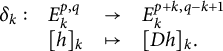
Applying this to
$h= f^{1}$
 , we obtain

Now, we show that
$[f^{1}]_k$
 is a cocycle representing a non zero class in
$(E_{k+1}^{*,*}, \delta _k)$
is a cocycle representing a non zero class in
$(E_{k+1}^{*,*}, \delta _k)$
 .
.
On one hand, since,

and
$D^2f^1 = 0,$
 we have, by degree reason,
$D_k(h^{0}_{1}- D_{k+1}\xi _1) =0$
we have, by degree reason,
$D_k(h^{0}_{1}- D_{k+1}\xi _1) =0$
 . So, being
$|h^{0}_{1}- D_{k+1}\xi _1| = N+1$
. So, being
$|h^{0}_{1}- D_{k+1}\xi _1| = N+1$
 , there is some
$\xi _2\in A$
, there is some
$\xi _2\in A$
 such that
$h^{0}_{1}- D_{k+1}\xi _1 = D_k\xi _2$
such that
$h^{0}_{1}- D_{k+1}\xi _1 = D_k\xi _2$
 . Therefore, using the isomorphism
$E_k^{p+k,q-k+1} \cong H^{p+q+1}(A,D_k)$
. Therefore, using the isomorphism
$E_k^{p+k,q-k+1} \cong H^{p+q+1}(A,D_k)$
 , we deduce that
$\delta _k[f^{1}]_k=0$
, we deduce that
$\delta _k[f^{1}]_k=0$
 and
$[f^{1}]_k$
and
$[f^{1}]_k$
 represents a cohomology class in
$E_{k+1}^{p,q}$
represents a cohomology class in
$E_{k+1}^{p,q}$
 .
.
On the other hand, if
$[f^1]_k = \delta _k[g]_k= [Dg]_k$
 , for some
$g\in Z_k^{p-k+1,q+k-2}$
, for some
$g\in Z_k^{p-k+1,q+k-2}$
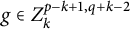 , then
${[f^1 - Dg]_k =0}$
, then
${[f^1 - Dg]_k =0}$
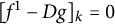 in
$E_k^{p,q}$
in
$E_k^{p,q}$
 or equivalently, using (2.6), the component
$pr_{-k+1}\circ (f^1 - Dg)$
or equivalently, using (2.6), the component
$pr_{-k+1}\circ (f^1 - Dg)$
 in
$\Lambda ^p V$
in
$\Lambda ^p V$
 of
$f^1 - Dg$
of
$f^1 - Dg$
 , which we denote by
$(f^1 - Dg)_{\Lambda ^p V}$
, which we denote by
$(f^1 - Dg)_{\Lambda ^p V}$
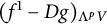 , decomposes as
$(h_1 + Dh_2)_{\Lambda ^p V}$
, decomposes as
$(h_1 + Dh_2)_{\Lambda ^p V}$
 in
$Z^{p+1,q-1}_{k-1} + B_{k-1}^{p,q}$
in
$Z^{p+1,q-1}_{k-1} + B_{k-1}^{p,q}$
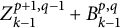 . Clearly, only the first term
$D_k$
. Clearly, only the first term
$D_k$
 of D acts and then we have
${(f^1 - D_kg)_{\Lambda ^p V}= (D_k{h_2})_{\Lambda ^p V}}$
of D acts and then we have
${(f^1 - D_kg)_{\Lambda ^p V}= (D_k{h_2})_{\Lambda ^p V}}$
 . Hence, applying
$D_k$
. Hence, applying
$D_k$
 , we get
$D_kf^1_{\Lambda ^pV} = D_kf_{\Lambda ^pV} - D_k{\xi _1}_{\Lambda ^pV}= - D_k{\xi _1}_{\Lambda ^pV}=0,$
, we get
$D_kf^1_{\Lambda ^pV} = D_kf_{\Lambda ^pV} - D_k{\xi _1}_{\Lambda ^pV}= - D_k{\xi _1}_{\Lambda ^pV}=0,$
 that is,
$h_0^0 =0$
that is,
$h_0^0 =0$
 . This contradicts the fact that
$f\in Z_{k-1}^{p,q}$
. This contradicts the fact that
$f\in Z_{k-1}^{p,q}$
 , hence
$[f^{1}]_k$
, hence
$[f^{1}]_k$
 is indeed a cocycle representing a non zero class in
$(E_{k+1}^{*,*}, \delta _k)$
is indeed a cocycle representing a non zero class in
$(E_{k+1}^{*,*}, \delta _k)$
 .
.
We continue by reconsidering the above expression of
$Df^1$
 which actually is as follows:

This can be resumed (for the same t due again to degree reason) as

where
$h_1^1 = h^{0}_{1}- D_{k+1}\xi _1 = D_k\xi _2$
 .
.
We then introduce
$f^2 =f^1 - \xi _2 = f - \xi _1 - \xi _2$
 and show, using the same argument, that
$[f^{2}]_k$
and show, using the same argument, that
$[f^{2}]_k$
 is a cocycle representing a non zero class in
$E_{k+2}^{p,q}$
is a cocycle representing a non zero class in
$E_{k+2}^{p,q}$
 . Moreover, we may write

where
$h_2^2 = h^{2}_{0}- D_{k+2}\xi _1 - D_{k+1}\xi _2$
 .
.
We continue this process until we reach the stage s where the spectral sequence degenerates. This induces the generating class of
$E_{\infty }^{p,q} =E_{s}^{p,q}$
 represented by
$f^s = f - \xi _1 - \xi _2 - \cdots - \xi _s$
represented by
$f^s = f - \xi _1 - \xi _2 - \cdots - \xi _s$
 . Thus, using the aforementioned identification
$E_{\infty }^{p,q} = \mathrm{Ext}_{(\Lambda V,d)}^{p+q}(\mathbb {K},(\Lambda V,d))$
. Thus, using the aforementioned identification
$E_{\infty }^{p,q} = \mathrm{Ext}_{(\Lambda V,d)}^{p+q}(\mathbb {K},(\Lambda V,d))$
 , we take
$[f^s]$
, we take
$[f^s]$
 as the required generating class of
$\mathrm{Ext}_{(\Lambda V,d)}^{p+q}(\mathbb {K},(\Lambda V,d))$
as the required generating class of
$\mathrm{Ext}_{(\Lambda V,d)}^{p+q}(\mathbb {K},(\Lambda V,d))$
 .
.
As an application, we present below an immediate proof of [Reference Acharqy and Rami1, Theorem 2] which we recall here for convenience.
Theorem 4.3 Let X be a rationally elliptic space. Then, the spectral sequence (4.4) degenerate at t, hence,
$L_0(X) = l_0(X) = t-1$
 .
.
Proof 2 The above algorithm shows that the spectral sequence (2.11) degenerates exactly at
$s=t$
 , hence
$L_0(X) = t-1$
, hence
$L_0(X) = t-1$
 . Because the evaluation map
$ev_{(\Lambda V,d)}([f^t]) = [f^t(1)]$
. Because the evaluation map
$ev_{(\Lambda V,d)}([f^t]) = [f^t(1)]$
 coincides with the fundamental class obtained from the Milnor–Moore spectral sequence (2.9) via the Lechuga–Murillo algorithm [Reference Boutahir and Rami2, Theorem 2] (see Remark 4.2), the same index t governs the degeneration of (2.9). Consequently,
$l_0(X)=t-1$
coincides with the fundamental class obtained from the Milnor–Moore spectral sequence (2.9) via the Lechuga–Murillo algorithm [Reference Boutahir and Rami2, Theorem 2] (see Remark 4.2), the same index t governs the degeneration of (2.9). Consequently,
$l_0(X)=t-1$
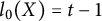 as well.
4.1.2 The invariant
$\mathrm {R}_0(\Lambda V,d)$

Recall from [Reference Rami18] that the second author introduced, in terms of (2.11), the invariant

This is given in spirit of Toomer’s invariant which in turn is given in terms of (2.9) by

An equivalent definition of
$\mathrm {R}_0(\Lambda V,d)$
 given in [Reference Rami18, Remark 3.4], in terms of the generating class
$\Omega $
given in [Reference Rami18, Remark 3.4], in terms of the generating class
$\Omega $
 of
$\mathrm{Ext}^{*}_{(\Lambda V,d)}(\mathbb {K},(\Lambda V,d))$
of
$\mathrm{Ext}^{*}_{(\Lambda V,d)}(\mathbb {K},(\Lambda V,d))$
 , is as follows:

Our first result in this section gives another proof of [Reference Acharqy and Rami1, Theorem 1] which relies on the algorithm defining
$f^t$
 .
.
Theorem 4.4 Let X be a rationally elliptic CW-complex. Then,
$\mathrm {R}_0(X)=e_0(X)=\mathrm{cat}_0(X).$

Proof 3 By hypothesis, X being elliptic, its Sullivan minimal model
$(\Lambda V,d)$
 is elliptic hence
$\dim V < \infty $
is elliptic hence
$\dim V < \infty $
 and
$\dim H(\Lambda V,d)<\infty $
and
$\dim H(\Lambda V,d)<\infty $
 . In particular,
$(\Lambda V,d_k)$
. In particular,
$(\Lambda V,d_k)$
 is a Gorenstein algebras, that is,

where the unique bi-degree
$(p',q')$
 derived from the filtration (2.10) satisfies
$p'+q'=N$
derived from the filtration (2.10) satisfies
$p'+q'=N$
 , the formal dimension of
$(\Lambda V,d)$
, the formal dimension of
$(\Lambda V,d)$
 . By the convergent spectral sequence (2.11), we have also

This implies
$\mathrm {R}_0(\Lambda V,d) = p' = \mathrm {R}_0(X)$
 (cf. §6 for more explanation).
Next, since the chain evaluation map (2.4):

preserves the filtrations (2.10) and (2.8), in homology, it induces a morphism between the convergent spectral sequences (2.11) and (2.9). Hence, the
$E_\infty $
 morphism

is indeed an isomorphism (recall that
$\dim H^{N}(\Lambda V,d)=1$
 ). By the above theorem,
$L_0(\Lambda V,d) = l_0(\Lambda V,d)$
). By the above theorem,
$L_0(\Lambda V,d) = l_0(\Lambda V,d)$
 therefore, by (1.1), we obtain
$e_0{(\Lambda V,d)} = p'=e_0(X)$
therefore, by (1.1), we obtain
$e_0{(\Lambda V,d)} = p'=e_0(X)$
 and thus,
$\mathrm {R}_0(X)=e_0(X)=\mathrm{cat}_0(X).$
and thus,
$\mathrm {R}_0(X)=e_0(X)=\mathrm{cat}_0(X).$

To illustrate, we apply the algorithm to a specific Sullivan model.
Example 4.5 Let us reconsider the Sullivan model from example 3.1:
$(\Lambda x_{2},x_{4},y_{5},y_{7}, d)$
 , with differentials

Its formal dimension is
$N=8$
 . The quadratic associated model
$(\Lambda V,d_{2})$
. The quadratic associated model
$(\Lambda V,d_{2})$
 is a pure but non-elliptic, with top class
$\omega =[x_{2}^{2}x_{4}]$
is a pure but non-elliptic, with top class
$\omega =[x_{2}^{2}x_{4}]$
 and
$H^8(\Lambda V,d_{2})=\mathbb Q[x_2^4]$
and
$H^8(\Lambda V,d_{2})=\mathbb Q[x_2^4]$
 . We apply the algorithm of §4 to the Eilenberg–Moore spectral sequence

Starting from the generating class
$\Omega _2=[f]$
 of
$\mathrm{Ext}^{(2,6)}_{(\Lambda V,d_{2})}(\mathbb {K};\,(\Lambda V,d_{2}))$
of
$\mathrm{Ext}^{(2,6)}_{(\Lambda V,d_{2})}(\mathbb {K};\,(\Lambda V,d_{2}))$
 obtained in Example 3.2 (with
$f(1)=2x_4^2$
obtained in Example 3.2 (with
$f(1)=2x_4^2$
 ), the Lechuga–Murillo procedure yields, after three successive corrections
$\xi _1,\xi _2,\xi _3$
), the Lechuga–Murillo procedure yields, after three successive corrections
$\xi _1,\xi _2,\xi _3$
 , a generating class
$[f^3]$
, a generating class
$[f^3]$
 of
$\mathrm{Ext}^{8}_{(\Lambda V,d)}(\mathbb {K};\,(\Lambda V,d))$
of
$\mathrm{Ext}^{8}_{(\Lambda V,d)}(\mathbb {K};\,(\Lambda V,d))$
 such that
$Df^3=0$
such that
$Df^3=0$
 and
$[f^3]$
and
$[f^3]$
 is not a D-coboundary. Consequently,
$t=3$
is not a D-coboundary. Consequently,
$t=3$
 ,
$L_0(X)=t-1=2,$
,
$L_0(X)=t-1=2,$
 and
and

5 A basis of
$\mathrm{Ext}_{(\Lambda V,d)}(\mathbb {K},(\Lambda V,d))$
from that of
$Ext_{(\Lambda V,d_{\sigma })}(\mathbb {K};(\Lambda V,d_{\sigma }))$


In this section, we lift the generating class from the pure model
$(\Lambda V,d_{\sigma })$
 to the full model
$(\Lambda V,d)$
to the full model
$(\Lambda V,d)$
 using the odd-Eilenberg–Moore spectral sequence. The proof of Theorem 1.1 is completed here, showing that
$[(f_{k,\sigma }^t)^l(1)]$
using the odd-Eilenberg–Moore spectral sequence. The proof of Theorem 1.1 is completed here, showing that
$[(f_{k,\sigma }^t)^l(1)]$
 is precisely the fundamental class of
$(\Lambda V,d)$
is precisely the fundamental class of
$(\Lambda V,d)$
 .
.
Let
$(\Lambda V,d)$
 be a minimal Sullivan model with finite-dimensional V. Following Halperin [Reference Félix, Halperin and Thomas7, Reference Halperin9], we introduce a bi-grading on
$\Lambda V$
be a minimal Sullivan model with finite-dimensional V. Following Halperin [Reference Félix, Halperin and Thomas7, Reference Halperin9], we introduce a bi-grading on
$\Lambda V$
 by setting
$Q= V^{\text {even}}$
by setting
$Q= V^{\text {even}}$
 and
$P = V^{\text {odd}}$
and
$P = V^{\text {odd}}$
 . Specifically,

where n is the total degree and
$p=n+q$
 the filtering degree. The filtration is

This filtration induces a convergent spectral sequence whose
$E_0$
 -term is the pure Sullivan model
$(\Lambda V,d_{\sigma })$
-term is the pure Sullivan model
$(\Lambda V,d_{\sigma })$
 . The differential
$d_{\sigma }$
. The differential
$d_{\sigma }$
 satisfies

with
$d_{\sigma }(V^{\text {even}})=0$
 and
$d_{\sigma }(V^{\text {odd}})\subseteq \Lambda V^{\text {even}}$
and
$d_{\sigma }(V^{\text {odd}})\subseteq \Lambda V^{\text {even}}$
 . The associated spectral sequence

is called the odd spectral sequence. Its main consequence is that
$(\Lambda V,d)$
 is elliptic if and only if
$(\Lambda V,d_{\sigma })$
is elliptic if and only if
$(\Lambda V,d_{\sigma })$
 is elliptic. Thus, as already noted in §2, any Sullivan model satisfying the above condition is called a pure Sullivan model.
We now consider the acyclic closure
$(\Lambda V\otimes \Lambda sV, d)\stackrel {\simeq }{\rightarrow } (\mathbb {Q},0)$
 . The differential D on
$A=\mathrm{Hom}_{\Lambda V}(\Lambda V\otimes \Lambda sV;\Lambda V)$
. The differential D on
$A=\mathrm{Hom}_{\Lambda V}(\Lambda V\otimes \Lambda sV;\Lambda V)$
 is
is

The pure differential
$d_{\sigma }$
 induces
$D_{\sigma }$
induces
$D_{\sigma }$
 on A defined by

Therefore, we obtain the relation
$D(f)=D_{\sigma }(f)+\varphi (f),\; \forall f\in A$
 with
$\varphi (f) = (D-D_{\sigma })(f)$
with
$\varphi (f) = (D-D_{\sigma })(f)$
 .
.
In [Reference Rami18], denoting

the second author introduced on
$A^n=\mathrm{Hom}_{\Lambda V}^n(\Lambda V\otimes \Lambda sV,\Lambda V)$
 (
$n\geq 0$
(
$n\geq 0$
 ) the following filtration:

That is,
$f\in F^{p}A^{n}$
 if and only if
$f((\Lambda V\otimes \Lambda sV)^{r,s}) \subseteq (\Lambda ^{\geq p+n+s+r, *}V)^{n+s}$
if and only if
$f((\Lambda V\otimes \Lambda sV)^{r,s}) \subseteq (\Lambda ^{\geq p+n+s+r, *}V)^{n+s}$
 . Note that the differential on
$(\Lambda V\otimes \Lambda sV)^{r,s}$
. Note that the differential on
$(\Lambda V\otimes \Lambda sV)^{r,s}$
 preserves both s (total degree) and r (filtering degree). Thus, he obtains the following convergent spectral sequence, called the Ext-odd spectral sequence of
$(\Lambda V,d)$
preserves both s (total degree) and r (filtering degree). Thus, he obtains the following convergent spectral sequence, called the Ext-odd spectral sequence of
$(\Lambda V,d)$
 :
:

Since V is finite-dimensional, both
$(\Lambda V,d)$
 and
$(\Lambda V,d_{\sigma })$
and
$(\Lambda V,d_{\sigma })$
 are Gorenstein dga’s with the same formal dimension N. Consequently, there exists a unique bi-degree
$(p,q)$
are Gorenstein dga’s with the same formal dimension N. Consequently, there exists a unique bi-degree
$(p,q)$
 such that
$\mathrm{Ext}_{(\Lambda V,d_{\sigma })}^{*,*}(\mathbb {K},(\Lambda V,d_{\sigma }))= \mathrm{Ext}^{(p,-q)}_{(\Lambda V,d_{\sigma })}(\mathbb {K},(\Lambda V,d_{\sigma }))$
such that
$\mathrm{Ext}_{(\Lambda V,d_{\sigma })}^{*,*}(\mathbb {K},(\Lambda V,d_{\sigma }))= \mathrm{Ext}^{(p,-q)}_{(\Lambda V,d_{\sigma })}(\mathbb {K},(\Lambda V,d_{\sigma }))$
 is one-dimensional. Recall also that
$A:= \mathrm{Hom}_{\Lambda V}(\Lambda V\otimes \Lambda sV,\Lambda V).$
is one-dimensional. Recall also that
$A:= \mathrm{Hom}_{\Lambda V}(\Lambda V\otimes \Lambda sV,\Lambda V).$

Following the approach for the spectral sequence (2.11), we proceed to determine a generating class
$[h]$
 of
$\mathrm{Ext}^{p-q}_{(\Lambda V,d)}(\mathbb {K},(\Lambda V,d))$
of
$\mathrm{Ext}^{p-q}_{(\Lambda V,d)}(\mathbb {K},(\Lambda V,d))$
 from that, say
$[f]$
from that, say
$[f]$
 , of
$\mathrm{Ext}^{p,-q}_{(\Lambda V,d_{\sigma })}(\mathbb {K},(\Lambda V,d_{\sigma }))$
, of
$\mathrm{Ext}^{p,-q}_{(\Lambda V,d_{\sigma })}(\mathbb {K},(\Lambda V,d_{\sigma }))$
 . Using notation of §§1.4, we have
$f\in Z_{1}^{p,-q}$
. Using notation of §§1.4, we have
$f\in Z_{1}^{p,-q}$
 and
$|f|=N= p-q$
and
$|f|=N= p-q$
 , that is,
$f(\Lambda V\otimes \Lambda sV)^{r,s}\in F^{p+N+r+s}(\Lambda V)$
, that is,
$f(\Lambda V\otimes \Lambda sV)^{r,s}\in F^{p+N+r+s}(\Lambda V)$
 and
$Df(\Lambda V\otimes \Lambda sV)^{r,s}\subset F^{p+N+r+s+1}(\Lambda V).$
and
$Df(\Lambda V\otimes \Lambda sV)^{r,s}\subset F^{p+N+r+s+1}(\Lambda V).$

-
• First, assume $Df=0$
. If, moreover,
$f = Dg$
, for some
$g\in A^{N-1}$
, then
$f-D_{\sigma }(g) = (D-D_{\sigma })(g)$
is a
$D_{\sigma }$
-cocycle. Now, as
$|g|=N-1$
and
$d_{| {\Lambda V \otimes \Lambda sV}}$
sends
$(\Lambda V\otimes \Lambda sV)^{r,s}$
to
$(\Lambda V\otimes \Lambda sV)^{r-1,s+1}\oplus (\Lambda V\otimes \Lambda sV)^{\geq r,s+1}$
, g should send
${(\Lambda V\otimes \Lambda sV)^{r-1,s+1}}$
to
$F^{p+N+r+s}(\Lambda V)=F^{(p+1)+(N-1)+(r-1)+(s+1)}(\Lambda V)$
. This yields the following diagram: (5.5) $$ \begin{align} \begin{array}{ccc} (\Lambda V\otimes \Lambda sV)^{r,s} & \stackrel{{d_{\sigma}}_{|{\Lambda V \otimes \Lambda sV}}}{\longrightarrow} & (\Lambda V\otimes \Lambda sV)^{r-1,s+1} \\ \downarrow g & & g \downarrow \\ F^{(p+1)+(N-1)+r+s}(\Lambda V ) & \stackrel{{d_{\sigma}}_{|{\Lambda V}}}{\longrightarrow} & F^{p+N+r+s}(\Lambda V). \end{array} \end{align} $$
Therefore, $D_{\sigma }(g) = g\circ {d_{\sigma }}_{|{\Lambda V \otimes \Lambda sV}} + (-1)^N {d_{\sigma }}_{|{\Lambda V}}\circ g$
sends
$(\Lambda V\otimes \Lambda sV)^{r,s}$
to
$F^{p+N+r+s}(\Lambda V)$
. The same analysis give us the following diagram: (5.6) $$ \begin{align} \begin{array}{ccc} (\Lambda V\otimes \Lambda sV)^{r,s} & \stackrel{{(d-d_{\sigma})}_{|{\Lambda V \otimes \Lambda sV}}}{\longrightarrow} & (\Lambda V\otimes \Lambda sV)^{\geq r,s+1} \\ \downarrow g & & g \downarrow \\ F^{(p+1)+(N-1)+r+s}(\Lambda V) & \stackrel{{(d-d_{\sigma})}_{|{\Lambda V}}}{\longrightarrow} & F^{>p+N+r+s}(\Lambda V). \end{array} \end{align} $$
It follows that $f-D_{\sigma }(g) = (D-D_{\sigma })(g)$
sends
$(\Lambda V\otimes \Lambda sV)^{r,s}$
to
$F^{(p+1)+N+r+s}(\Lambda V)$
. So, if
$f-D_{\sigma }(g)$
is not a
$D_{\sigma }$
-coboundary, then
$[f-D_{\sigma }(g)]$
becomes a generating class of
$ \mathrm{Ext}^{*,*}_{(\Lambda V,d_{\sigma })}(\mathbb {K},(\Lambda V,d_{\sigma }))$
of bi-degree
$(p+1,q-1)$
, which contradicts uniqueness of
$(p,q)$
. We then conclude that if
$Df=0,$
then
$[f]$
is a generating class of
$ \mathrm{Ext}^{*,*}_{(\Lambda V,d)}(\mathbb {K},(\Lambda V,d))$
. -
• Second, assume that $Df\neq 0$
. Decompose
$Df$
as in the previous section: $$ \begin{align*} Df_{|(\Lambda V\otimes \Lambda sV)^{r,s}} = g_{0}^{0} + \cdots + g_{l}^{0}, \end{align*} $$where l is the greatest integer with $g_{l}^{0}\neq 0$
and each
$g_i^0$
sends
$(\Lambda V\otimes \Lambda sV)^{r,s}$
to
$(\Lambda V )^{p+N+s+r+i+1,*}$
. Let
$m= \mathrm{max}\{|v_i|,\; v_i\in V\}$
; by [Reference Félix, Halperin and Thomas7, Corollary 1, p. 441], we have
$2\leq m\leq 2N-1$
. The degree condition yields
$l\leq \frac {-N+m}{2}-(r+s+p+1)$
.
This decomposition extends to $Df$
so that: (5.7) $$ \begin{align} Df=h_{0}^{0}+\cdots+h_{l}^{0}. \end{align} $$
As in the above section, this is equivalent to:
(5.8) $$ \begin{align} Df((\Lambda V\otimes\Lambda sV)^{r,s})\subseteq (\Lambda V)^{p+N+s+r+1,*} \oplus\cdots\oplus (\Lambda V)^{p+N+s+r+l+1,*}. \end{align} $$
Now, using the fact $D^{2}f=0$
and by considering word length, we get
${D_{\sigma }(h_{0}^{0})=0}$
. Moreover, as
$|h_0^0| = |Df| = N+1$
, we have
$[h_0^0] =0,$
hence,
$h_{0}^{0}=D_{\sigma }\beta _{1}$
for some
$\beta _{1} \in A^N$
.The iterative construction of the correctors $\beta _j$
is analogous to the Lechuga–Murillo procedure described in §4, with the filtration (5.3) playing the role of the filtration (2.10). We therefore only sketch the main steps.To continue, we consider $f^{1}=f-\beta _{1}$
. Since,
$|\beta _1|=N$
,
$h_{0}^{0}=D_{\sigma }\beta _{1}$
, and
$h_0^0(\Lambda V\otimes \Lambda sV)^{r,s}\subseteq F^{p+N+r+s+1}(\Lambda V )$
, we have
$\beta _1(\Lambda V\otimes \Lambda sV)^{r,s}\subseteq F^{p+N+r+s+1}(\Lambda V )$
and
${(D-D_{\sigma })(\beta _1)(\Lambda V\otimes \Lambda sV)^{r,s}\subseteq F^{p+N+r+s+2}(\Lambda V )}$
(compare with g and
$(D-D_{\sigma })(g)$
in the diagrams (5.5) and (5.6), respectively). It follows that
$f^{1}(\Lambda V\otimes \Lambda sV)^{r,s}\subseteq F^{p+N+r+s+1}(\Lambda V )$
. Afterwards, since $$ \begin{align*}Df_1 =Df - D\beta_1 = (D-D_{\sigma})(f) - h_0^0 - (D-D_{\sigma})(\beta_1) = h_1^0 + \cdots + h_l^0 -(D-D_{\sigma})(\beta_1),\end{align*} $$we deduce that $Df^{1}(\Lambda V\otimes \Lambda sV)^{r,s}\subseteq F^{p+N+r+s+2}(\Lambda V)$
.
Next, expressing $F^{p+N+r+s+2}(\Lambda V ) = (\Lambda V) ^{\geq p+N+r+s+2, *}$
as the sum: $$ \begin{align*}F^{p+N+r+s+2} = (\Lambda V) ^{p+N+r+s+2, *} \oplus (\Lambda V) ^{p+N+r+s+3, *} \oplus \cdots \oplus (\Lambda V) ^{ p+N+r+s+l+1, *}(\Lambda V )\end{align*} $$we see that $(D-D_{\sigma })(\beta _1)$
may be decomposed as follows: $$ \begin{align*}(D-D_{\sigma})(\beta_1) = \beta_1^{(1)} + \beta_1^{(2)} + \cdots + \beta_1^{(l)},\end{align*} $$where $\beta _1^{(i)}$
, (
$1\leq i \leq l$
), is the component of
$(D-D_{\sigma })(\beta _1),$
which sends
${(\Lambda V\otimes \Lambda sV)^{r,s}}$
to
$(\Lambda V)^{p+N+r+s+i+1, *}$
. Therefore, we may write $$ \begin{align*}Df^1 = h_1^1 + h_2^1 = \cdots + h_l^1\end{align*} $$with $h_1^1 = h_1^0 - \beta _1^{(1)}$
. We then continue by analyzing the behaviors of
$f^1$
.
Again, using the equation $D^2f^1=0$
, we obtain some
$\beta _2\in A^{N}$
such that
$h_1^1 = D_{\sigma }\beta _2$
. This leads to
$f^2 = f^1-\beta _2 = f -\beta _1 - \beta _2$
. Similarly, we may show that
$\beta _2(\Lambda V\otimes \Lambda sV)^{r,s}\subseteq F^{p+N+r+s+2}(\Lambda V )$
and
$(D-D_{\sigma })(\beta _2)(\Lambda V\otimes \Lambda sV)^{r,s}\subseteq F^{p+N+r+s+3}(\Lambda V )$
, so that
$(D-D_{\sigma })(\beta _2)$
can be expressed as follows: $$ \begin{align*}(D-D_{\sigma})(\beta_2) = \beta_2^{(2)} + \beta_2^{(3)} + \cdots + \beta_2^{(l)},\end{align*} $$where $\beta _2^{(i)}$
, (
$2\leq i \leq l$
) is the component of
$(D-D_{\sigma })(\beta _2),$
which sends
${(\Lambda V\otimes \Lambda sV)^{r,s}}$
to
$(\Lambda V) ^{p+N+r+s+i+1, *}$
.
Continuing this process, we inductively define a sequence $(f^{j}, \beta _{j})\in A^N \times A^N$
for
$1\leq j \leq l$
with
$f^0 := f$
: $$ \begin{align*}\left \{ \begin{array}{l}\!\! f^{j}=f^{j-1}-\beta_{j}= f -\beta_1 -\beta_2 - \cdots - \beta_j\\ \!\! Df^{j}(\Lambda V\otimes \Lambda sV)^{r,s}\subseteq F^{p+r+s+N+j+1,*}\\ \!\! Df^j = h_j^j + h_{j+1}^j = \cdots + h_l^j. \end{array} \right. \end{align*} $$
It remains to show that $f^{l} = f -\beta _1 -\beta _2 - \cdots - \beta _l$
is a cocycle representing the generating class of
$\mathrm{Ext}^{p-q}_{(\Lambda V,d)}(\mathbb {K},(\Lambda V,d)).$
If $Df^l \neq 0$
, we proceed using the same procedure as in the previous section to obtain
$Df^l =h_l^l = D_\sigma \beta _{l+1}$
(for some
$\beta _{l+1}\in A^N$
). Additionally, based on the definition of l, we find that
$(D-D_{\sigma })(\beta _{l+1})=0$
. Consequently,
$Df^l =h_l^l = D\beta _{l+1}$
which implies
$D(f^l -\beta _{l+1})=0$
. Subsequently, we may substitute
$f^l -\beta _{l+1}$
for
$f^l$
.Next, we assume for simplicity that $Df^l= 0$
and show that
$f^l$
is not a coboundary.Assuming the contrary, i.e., there is some $g\in A^{N-1}$
such that
$f^l =Dg$
.On one hand, using (5.8), we see that
$$ \begin{align*}f((\Lambda V\otimes\Lambda sV)^{r,s})\subseteq (\Lambda V)^{p+N+s+r,*} \oplus \cdots \oplus (\Lambda V)^{p+N+s+r+l,*}.\end{align*} $$
Therefore, f decomposes as
$$ \begin{align*}f =f^0_0 + f_1^0 + \cdots + f_l^0,\end{align*} $$where $f_i^0(\Lambda V\otimes \Lambda sV)^{r,s})\subseteq (\Lambda V)^{p+N+s+r+i,*}$
.
On the other hand, since all terms of the spectral sequence (2.13) are one-dimensional (as graded vector spaces), we still have
$$ \begin{align*}f^l((\Lambda V\otimes\Lambda sV)^{r,s})\subseteq (\Lambda V)^{p+N+s+r,*} \oplus \cdots \oplus (\Lambda V)^{p+N+s+r+l,*}.\end{align*} $$
Thus, we should have
$$ \begin{align*}g((\Lambda V\otimes\Lambda sV)^{r,s})\subseteq (\Lambda V)^{p+N+s+r-1,*} \oplus \cdots \oplus (\Lambda V)^{p+N+s+r+l-1,*}\end{align*} $$so g also decomposes as
$$ \begin{align*}g =g^0_0 + g_1^0 + \cdots + g_l^0\end{align*} $$with $g_i^0((\Lambda V\otimes \Lambda sV)^{r,s})\subseteq (\Lambda V)^{p+N+s+r+i-1,*}$
.
It results, due to degree constraints, that $f_0^0 - \beta _1 = D_\sigma (g_0^0)$
. Hence, applying
$D_{\sigma }$
, we get
$D_\sigma \beta _1 = 0$
. That is,
$h_0^0 =0$
. This contradicts (5.8) or equivalently the fact that
$f\in F^p(A^N)$
and concludes the algorithm.









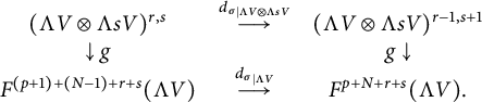



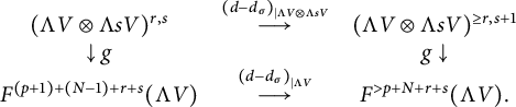






























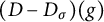













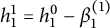















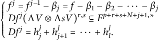




















Remark 5.1 A similar description given in Remark 4.2 may be used in terms of the following system of equations to determine
$f^l$
 :
:
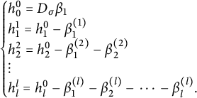
Alternatively, Lechuga–Murillo’s algorithm [Reference Lechuga and Murillo13, Reference Murillo15] can be applied to determine the
$\beta _i(1)$
 , starting with
$h_0^0(1)$
, starting with
$h_0^0(1)$
 instead of
$h_1^0(1)$
instead of
$h_1^0(1)$
 .
.
Here again, from
$f^l = f - \beta _1 - \beta _{2} - \cdots - \beta _l$
 , we obtain
$f^l(1) = f(1) - \beta _1(1) - \beta _{2}(1) - \cdots - \beta _l(1),$
, we obtain
$f^l(1) = f(1) - \beta _1(1) - \beta _{2}(1) - \cdots - \beta _l(1),$
 which indeed give us the fundamental class
$[f^l(1)] = ev_{(\Lambda V,d)}([f^l(1)])$
which indeed give us the fundamental class
$[f^l(1)] = ev_{(\Lambda V,d)}([f^l(1)])$
 of
$(\Lambda V,d)$
of
$(\Lambda V,d)$
 from that of
$(\Lambda V,d_{\sigma })$
from that of
$(\Lambda V,d_{\sigma })$
 .
.
Theorem 5.2 With the notation above,
$[f^{l}]$
 is the generating class of
$\mathrm{Ext}_{(\Lambda V,d)}(\mathbb {K},(\Lambda V,d))$
is the generating class of
$\mathrm{Ext}_{(\Lambda V,d)}(\mathbb {K},(\Lambda V,d))$
 .
.
We now prove Theorem 1.1
Proof 4 (Theorem 1.1)
Let
$f_{k,\sigma }(1)$
 be the representative of the top class of
$(\Lambda V,(d_{\sigma })_{k})$
be the representative of the top class of
$(\Lambda V,(d_{\sigma })_{k})$
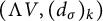 , from which we start our algorithm. This is indeed a coboundary since
$[f_{k,\sigma }(1)] = ev_{(\Lambda V,(d_{k})_{\sigma })}([f_{k,\sigma }])=0$
, from which we start our algorithm. This is indeed a coboundary since
$[f_{k,\sigma }(1)] = ev_{(\Lambda V,(d_{k})_{\sigma })}([f_{k,\sigma }])=0$
 [Reference Lechuga and Murillo12, Corollary 3]. But, as
$(\Lambda V,d_{\sigma })$
[Reference Lechuga and Murillo12, Corollary 3]. But, as
$(\Lambda V,d_{\sigma })$
 is itself elliptic,
$ev_{(\Lambda V,d_{\sigma })}([f_{k,\sigma }^t]) = [f_{k,\sigma }^t(1)]\neq 0$
is itself elliptic,
$ev_{(\Lambda V,d_{\sigma })}([f_{k,\sigma }^t]) = [f_{k,\sigma }^t(1)]\neq 0$
 , thus,
$(f_{k,\sigma }^t)(1)$
, thus,
$(f_{k,\sigma }^t)(1)$
 is not a coboundary. Clearly, the same holds for
$(f_{k,\sigma }^t)^l(1)$
is not a coboundary. Clearly, the same holds for
$(f_{k,\sigma }^t)^l(1)$
 by the convergence of the spectral sequence (2.12). Thus,
$[(f_{k,\sigma }^t)^l(1)]$
by the convergence of the spectral sequence (2.12). Thus,
$[(f_{k,\sigma }^t)^l(1)]$
 is the fundamental class of
$(\Lambda V,d)$
is the fundamental class of
$(\Lambda V,d)$
 and consequently,
$e_0(\Lambda V,d) = e_0([(f_{k,\sigma }^t)^l(1)])$
and consequently,
$e_0(\Lambda V,d) = e_0([(f_{k,\sigma }^t)^l(1)])$
 .
.
Example 5.3 Consider the Sullivan model
$(\Lambda (a,b,x,u,v,w), d)$
 with degrees

and differentials

The pure model
$(\Lambda V,\,d_{\sigma })$
 has fundamental class
$\omega _{0}=abxv-b^{2}xu$
has fundamental class
$\omega _{0}=abxv-b^{2}xu$
 and formal dimension
$N=14$
and formal dimension
$N=14$
 :
:

with fundamental class represented by
$\omega _{0}=abxv-b^{2}xu.$

Applying the algorithm of §3, one obtains the generating class
$[f]$
 of
$\mathrm{Ext}_{(\Lambda V,\,d_{\sigma })}(\mathbb Q,\,(\Lambda V,d_{\sigma }))$
of
$\mathrm{Ext}_{(\Lambda V,\,d_{\sigma })}(\mathbb Q,\,(\Lambda V,d_{\sigma }))$
 . The algorithm of §5 then lifts
$[f]$
. The algorithm of §5 then lifts
$[f]$
 to a generating class of
$Ext_{(\Lambda V,\,d)}(\mathbb Q,\,(\Lambda V,d))$
to a generating class of
$Ext_{(\Lambda V,\,d)}(\mathbb Q,\,(\Lambda V,d))$
 via the Ext-odd spectral sequence

The iterative correction process converges at
$l=1$
 : one corrector
$\beta _1$
: one corrector
$\beta _1$
 suffices, so that
$f^1=f-\beta _1$
suffices, so that
$f^1=f-\beta _1$
 satisfies
$Df^1=0$
satisfies
$Df^1=0$
 and
$[f^1]$
and
$[f^1]$
 is nonzero. Hence,
$[f^1]$
is nonzero. Hence,
$[f^1]$
 generates
$\mathrm{Ext}_{(\Lambda V,\,d)}(\mathbb Q,\,(\Lambda V,d))$
generates
$\mathrm{Ext}_{(\Lambda V,\,d)}(\mathbb Q,\,(\Lambda V,d))$
 , and
$[f^1(1)]$
, and
$[f^1(1)]$
 represents the fundamental class of
$(\Lambda V,d)$
represents the fundamental class of
$(\Lambda V,d)$
 .
.
6 Concluding remarks
-
(1) It is worth noting that if $(\Lambda V,d_{k})$
, hence
$(\Lambda V,(d_{k})_{\sigma })$
, is not elliptic, then
$(f_{k,\sigma }^t)^l(1)$
is not necessarily the representative that gives the exact value of
$e_0(X)$
. Indeed, as shown in the proof of Theorem 1.1, when the representative
$f_{k,\sigma }(1)$
of the top class of
$(\Lambda V,(d_{\sigma })_{k})$
is a coboundary, since
$(\Lambda V,d_{\sigma })$
is itself elliptic,
$(f_{k,\sigma }^t)(1)$
is not a coboundary as is
$(f_{k,\sigma }^t)^l(1)$
by the convergence of the spectral sequence (2.12). Thus,
$[(f_{k,\sigma }^t)^l(1)]$
is the fundamental class of
$(\Lambda V,d).$
It follows from the algorithm that, if $(p,q)$
designates the bi-degree of
$f_{k,\sigma }$
, then
$(f_{k,\sigma }^t)(1)\in \Lambda ^{\geq p}V$
and also
$(f_{k,\sigma }^t)^l(1)\in \Lambda ^{\geq p}V$
. By [Reference Boutahir and Rami2, Theorem 2], the fundamental class
$\omega \in H^N(\Lambda V,d)$
that results from some class
$\omega _{0} \in H^N(\Lambda V,(d_{\sigma })_{k})$
should be represented by
$\alpha \in \Lambda ^{\geq p'}V$
with
$p'\geq p$
. Thus,
$e_0(\Lambda V,d) =p'\geq p$
. -
(2) In the case, where $(\Lambda V,(d_{k})_{\sigma })$
is elliptic,
$[f_{k,\sigma }(1)]\in H^N(\Lambda V,(d_{\sigma })_{k})$
is the fundamental class of
$H^N(\Lambda V,(d_{\sigma })_{k})$
. Using the algorithm in §4, this persists to yield the fundamental class
$[f_{k,\sigma }^t(1)]\in H^N(\Lambda V,d_{\sigma })$
, and using the algorithm in §3, we get the desired fundamental class
$[(f_{k,\sigma }^t)^l]$
of
$(\Lambda V,d)$
. It follows that
$e_0(\Lambda V,(d_{\sigma })_{k}) = e_0(\Lambda V,d_{\sigma }) = e_0(\Lambda V,d)$
. This is determined by the explicit formula [Reference Lechuga and Murillo13, Theorem 6]: $$ \begin{align*}e_0(\Lambda V,(d_{\sigma})_{k}) = \dim{V^{odd}} + (k-2)\dim{V^{even}}.\end{align*} $$
This demonstrates the extensibility of our method to the general case.
-
(3) For details on the requirements imposed to accomplish the algorithm of §4, see Example 4.5. From this example, we can see the NP-hard complexity proven in [Reference Lechuga and Murillo11, Theorem 2] when determining this type of invariant.

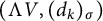


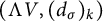









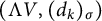








 Open access

