Where Is Polygamy in the World?

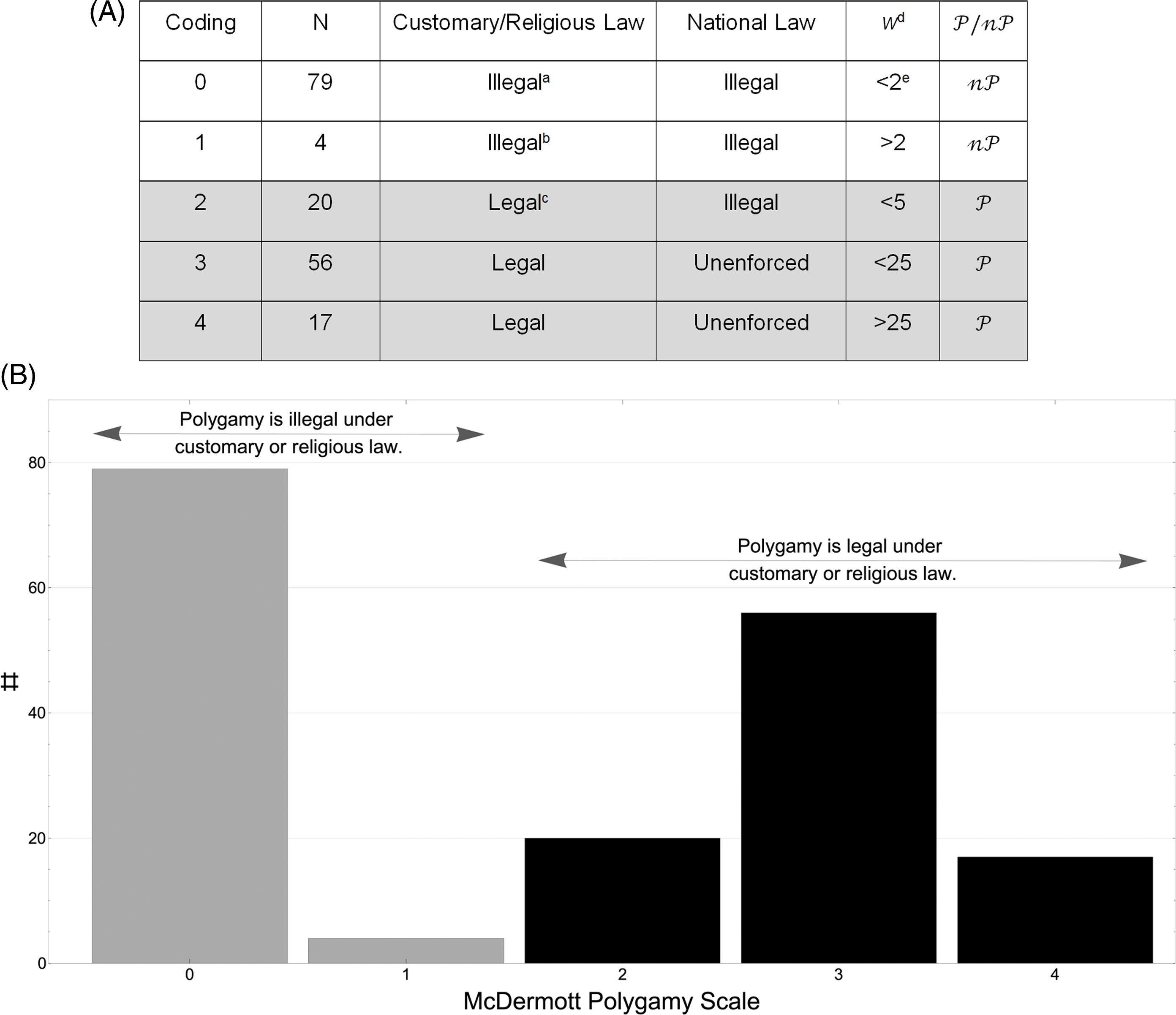
The most comprehensive global survey of contemporary polygamy is Rose McDermott’s (Reference McDermott2010). Combining assessments of laws, practices, and w, a measure of plural marriage prevalence, McDermott codes each of 176 nations on an integer scale between 0 and 4 (see figure 1A). ^{Footnote 6} Though a distinction on the basis of customary or religious law would seem at first glance to have no more or less gravitas than one made on the basis of national law, the histogram in figure 1B suggests that the former is weightier. We observe that the distribution of states is bimodal, cleaving along the line of legality in customary or religious law. This separates 4.1 billion people in 93 ${\cal P}$ -states where polygamy is legal under such law from 3.3 billion people in 83 ${\cal nP}$ -states where it is not.

Figure 1.

McDermott’s polygamy scale: (A) tabulation and (B) histogram. Notes: 1A: (a) Multiple cohabitations: <2 percent; (b) multiple cohabitations: >2 percent; (c) only applies to select minorities and/or within enclaves; (d) w is the fraction, specified in percent, of women in plural marriages; and (e) no US agency compiles statistics on covert polygamous marriages. One source has reported, without documentation, that 50,000 to 100,000 Muslims live in polygamous households (Hagerty Reference Hagerty2008). Another says, also without documentation, that 50,000 to 100,000 Black Muslims live in polygamous relationships (Al-Krenawi Reference Al-Krenawi2014). From these it seems fair to estimate that no more than 0.1 percent of American marriages are polygamous. In figure 1B, the vertical axis label (#) signifies the number of states in each classification category. The world according to McDermott’s coding scheme is evidently bimodal, cleaving along the line of customary and religious law’s view of polygamy.

We begin by focusing on polygamy’s molding of social convention. Following the lead of philosopher and social theorist David Lewis, we understand convention to be a normative behavior—that is one accompanied by could, would, or should—that is adhered to by almost all members of society (Reference Lewis1969). The requirement of near-universal adherence, in conjunction with the fact that human socialization begins in infancy and is well-established by adolescence, suggests that convention may change only on a timescale of generations. That being the case, whatever the convention is today, it is the consequence of events and practices that transpired long ago. While laws—customary, religious, or national—likely reflect convention, contemporary law cannot itself be the source of contemporary convention. The twentieth century’s roiling social upheavals were often accompanied by new or unfamiliar legal systems. We can expect, therefore, that contemporary law is out of step with convention in some states. As a predictor of contemporary convention, the ${\cal P}/{\cal nP}\;$ classification based on contemporary customary and religious law is likely to be inferior to such a classification made on the basis of customary and religious law in 1900. This warrants some changes to the ${\cal P}/{\cal nP}$ classification we have just made on the basis of contemporary law per McDermott’s Polygyny Scale. We describe these changes in the following five paragraphs.

Polygamy was legal under customary law as recently as 1999 in Azerbaijan, 1990 in Laos, 2015 in Myanmar, and 1956 in Tunisia. Though they are classified as ${\cal nP}$ in the McDermott coding, we designate them ${\cal P}$ . China is reportedly free of polygamy today though it was prevalent there from the ancient past until the time of Mao (Lee and Feng Reference Lee and Wang2001; Zurndorfer Reference Zurndorfer and Kam2016). Consequently, China is ${\cal P}$ , and so too is Mongolia, which only won its independence from China in 1921.

On the other hand, McDermott classifies Singapore as 2, and therefore ${\cal P}$ in our system. But it was a small British colony in 1900 whose nearly hundredfold population growth in the intervening years qualifies it, in our view, as a new country whose norms are not typical of other ${\cal P}$ -states. For this reason, we classify Singapore as ${\cal nP}$ .

We must classify the Muslim-majority Balkans (Albania and Kosovo) as ${\cal P}$ , and also Bosnia and Macedonia where Muslims comprise about 40 percent of the population. ^{Footnote 7} Finally, Fiji is a McDermott 0, though its long tradition of Chiefly Polygamy, irrespective of contemporary law, makes it ${\cal P}$ (Luker Reference Luker2015).

In the Muslim-majority Russian Republic of Chechnya, civil law prohibiting polygamy gives way to customary law permitting it (Tetrault-Farber Reference Tetrault-Farber2015). ^{Footnote 8} In McDermott’s system, Russia is a 2 and therefore ${\cal P}$ . But Russia is historically Orthodox, and Christendom has been monogamous since its earliest days under Roman rule where polygamy was at first not-normative and then later a crime (Witte Reference Witte2015: 104–14). The overwhelmingly dominant convention in Russia is thus monogamy. We classify it as ${\cal nP}$ .

In the Americas, Belize, Suriname, and Haiti are the only states that have laws, customary or civil, that permit or at least tolerate polygamy, and are thus ${\cal P}$ . By contrast, Guyana is a McDermott 0, but UNICEF reports that the plural marriage fraction there is 4 percent (2014). ^{Footnote 9} Accordingly, Guyana belongs among the ${\cal P}$ -states. ^{Footnote 10}

By this revised coding, approximately 5.5 billion people live under the influence of ${\cal P}$ and 2.0 billion live without such influence in ${\cal nP}$ . The global distribution of our revised ${\cal P}/{\cal nP}$ is shown in map 1, and a complete list is provided in the appendix. ^{Footnote 11}

Map 1.

World map of 102 ${\cal P}$ -states (in gray) and 75 ${\cal nP}$ -states (in white).

The Social Conventions of Polygamous Society

Polygamy is an asymmetric marriage contract—formal or informal, secular or religious, legal or illegal—that deprives the bride of the right of further marriage while preserving that right for the groom. Even in societies where it is permitted, generally fewer than one in three married men are polygamous, and more typically, fewer than one in ten. ^{Footnote 12} Though seemingly rare, the mere possibility of such asymmetric two-party contracts requires the tacit approval of most members of the community and supporting institutions that extend far beyond the sphere of the parties. Social conventions consistent with those contracts and their institutions will affect almost everyone within the sphere of permission. The driving mechanisms of polygamous convention and their consequences are the subject of this section.

In the 1710 edition of Transactions of the Royal Society, the world’s first scientific journal, Dr. John Arbuthnot (Reference Arbuthnot1710: 186–90) reported on the relative birth rates of girls and boys, finding them approximately equal, a conclusion supported by contemporary data as shown in figure 2. He also noted that, “where Males and Females are in equal number, if one man takes twenty wives, nineteen must live in celibacy, which is repugnant to the design of Nature.” He would have had no firsthand experience of polygamy in European society, though he would have known polygamy was common in Africa, and he might also have known something about its prevalence in the Near East, as did his contemporary Montesquieu (2008 [1721]), or in the Far East, as had been reported by Marco Polo in the thirteenth century (Reference Polo1958: Book 1, Chapter 52). He may be forgiven, then, his inference about celibacy, which is strictly correct only if marriage is restricted to parties of the same age. But his demography is sound and it bears heavily on polygamy. So long as men may take more than one wife, and women may not do the same, and so long as the male-to-female sex ratio at the age of puberty is not much less than unity—a condition that is satisfied everywhere—then polygamy creates a chronic scarcity of marriageable females.

Figure 2.

Male-to-female sex ratios for 177 nations. Notes: (A) Sex ratios in the first four years of life and (B) sex ratios in the first decade after puberty. Means and medians for both age groups are about 1.05. Population weighted means are larger by about 0.03 owing to sex ratios greater than 1.12 in China and India. Five states—Qatar, UAE, Bahrain, Maldives, and Kuwait—have sex ratios after puberty exceeding 1.2, a fact that may be attributed to a preference for males in their immigrant workforces.

Being that scarcity is at the root of economic behavior, the economist’s imagination is not tested by the proposition that women in polygamous society are traded like any other commodity. Nor is it tested by the proposition that the chronic scarcity influences economic outcomes in polygamous society relative to monogamous societies that do not face that particular scarcity. Whether that differential is large or small, or positive or negative remains to be determined. In this section we elucidate how a chronic scarcity of marriageable females molds social convention and promotes the commodification of all women.

When a community is struck by famine or drought, historical experience shows that those with access to scarce essentials often hoard them and those who don’t have access either maraud for them or suffer. To the extent possible or desirable, state and private institutions distribute the necessities from stockpiles to ameliorate the suffering and to protect the interests of the politically powerful. If scarcity and suffering mount, the afflicted grow more restive, flee, or even die. Where redistribution fails to quell civil disturbances, state and private militias may do so. But such scarcities often originate in the weather, and like the weather they pass, first coming and then going. As with recollections of a great blizzard, the transient scarcity fades, and it does so without engendering materially permanent behavioral change for almost all members of the group, which is requisite for our definition of convention.

Chronic scarcity is altogether different. It does not come and go like the weather. It comes and stays on a timescale of centuries, like climate. Within a few generations, no living person can recall the world before the scarcity took hold. ^{Footnote 13} If the scarcity does not pose an existential threat, or if alternatives can be found to alleviate the most dire of its consequences, then conventions adjust to the new normal and the old cultural system passes into legend.

Marriageable women are not like food or water; a man in search of a wife will not die in weeks for lack of a mate. However, the reproductive instinct is intrinsic to all life, leading us to expect that the logic of the market will apply where marriageable women are scarce, as they are wherever polygamy is permitted. In the following, we identify 11 different conventions that we hypothesize will be overrepresented in polygamous society. Because other factors independent of polygamy may give rise to these same conventions in nonpolygamous society, we do not expect that these conventions are necessarily absent there. We do, however, expect that they will be less prevalent there.

First, where marriageable women are a scarce commodity, we expect that they will be more highly valued in the marriage market, and that families with daughters will approve their marriage only for a price. Unlike dowry, which is a transfer of assets from the bride’s family to the married couple, bride price is a transfer of assets from the groom or the groom’s family to the bride’s family. Typically, these accrue to her father. Valerie Hudson (Reference Hudson2016) has developed an 11-point grading system for the full range of at-marriage wealth transfers: 0 signifies that neither dowry nor bride price is common; 1 to 5 signifies a range of dowry conventions; and 6 to 10 signifies a range of bride price conventions. By her design, circumstances for women are less favorable as the index value increases. We divide her sample of 173 states into groups according to the ${\cal P}/{\cal nP}$ classification. By visual inspection, the distributions of wealth transfer conventions within ${\cal P}$ and ${\cal nP}$ , figures 3A and 3B, respectively, are so dissimilar as to be distinct. Furthermore, bride price, we observe, is a practice all but unique to polygamous society. ^{Footnote 14}

Figure 3.

Hudson’s index of wealth transfers at marriage. Notes: (A) The distribution of wealth transfers at marriage per Hudson’s index in 73 ${\cal nP}$ states. (B) The distribution of wealth transfers at marriage per Hudson’s index in 100 ${\cal P}$ states. (C) The cumulative distribution functions of the ${\cal P}$ and ${\cal nP}$ distributions. The maximum difference, $\delta $ , of these is approximately 0.9, generating a vanishingly small p _ks , from which we conclude that the distributions are distinct, as expected.

As a quantitative diagnostic of similarity between two distributions, economists have long employed the Kolmogorov–Smirnov or KS test (Dagum Reference Dagum1980). It hinges on the observation that two distributions are similar only if their cumulative distribution functions (CDF) differ by at most a small amount, $\delta $ . The KS test generates an estimate of the probability that two distributions are the same. That probability, ${p_{KS}}$ , is exponential in the term $ - {\cal N}{\delta ^2}$ , where ${\cal N}\;$ is of the order of the number of elements in the smaller of the two distributions. ${p_{KS}}$ is therefore nonnegligible only if $\delta \le 1/\surd {\cal N}$ . In the case at hand, ${\cal N} \cong 70$ , so ${p_{KS}}$ is nonnegligible only if $\delta \le 0.12$ . The CDFs of ${\cal P}$ and ${\cal nP}$ distributions of at-marriage wealth transfers are shown in figure 3C. The corresponding $\delta \cong 0.9$ , so ${p_{KS}}$ is vanishingly small. We conclude, therefore, that the ${\cal P}/{\cal nP}$ dichotomy gives rise, in the case of wealth transfers at marriage, to distinctly different conventions, as we hypothesized.

We claim, if contentiously, that polygamy causes, or is one of the causes of the convention we call bride price, or ${\cal P} \rightarrow B$ in the notation of causal inference theory (Pearl and McKenzie Reference Pearl and Dana2018: 128ff). By this we mean that (1) there exists a mechanism by which ${\cal P}$ effects B ; (2) ${\cal P}$ is highly correlated with B ; (3) ${\cal P}$ precedes B ; and (4) there is no confounding factor Z that induces changes to both ${\cal P}$ and B . Having already demonstrated (1) and (2), we proceed to investigate (3) and (4).

In The Histories of Herodotus (fifth century BCE) polygamy was present throughout Eurasia and Africa, though it was absent in Athens and possibly other Greek city-states. This absence is consistent with Diane Hughes’s assessment of the absence of bride price in the same sources (Reference Hughes1978: 262–63). Polygamy was present, too, among the Greeks in The Iliad, as well as documented in eighth-century BCE China (Golden Reference Golden2002: 49). Thus, polygamy was present everywhere in the historical record at least 2,700 years before the present. ^{Footnote 15} If a nonpolygamous society existed before that time, it left no record and its impact on marriage structure was transient. Society emerged in the presence of preexisting polygamy. ^{Footnote 16} It follows that the polygamy-born scarcity of marriageable females was a fact on the ground for emergent society to manage, just as it had to manage scarcities of food, water, and shelter. The solutions to those management challenges are social conventions, bride price being one example. The temporal or chronological primacy of ${\cal P}$ relative to all convention rules out the existence of a conventional confounder Z that causes B . Regarding the existence of a natural confounder, that is, one born of climate or geography, the latter is ruled out because geography is a constant over the Holocene. We rule out climate as a confounder because polygamy was everywhere, irrespective of climate, by the earliest evidence.

The evidence of mechanism, correlation, and chronology, and the absence of evidence of confounders, all point to polygamy being the cause of bride price. ^{Footnote 17} Variations on these arguments apply for the other 10 conventions described in the following text. ^{Footnote 18} Table 1 summarizes the descriptive statistics of the 11 conventions we discuss in this article. We refer to these by name or by line item, for example #1 in lieu of bride price.

Table 1.

Eleven social conventions and descriptive statistics of their distributions in ${\cal P}$ and ${\cal nP}$

Note: Data tables and their sources are provided in the supplementary appendix.

Just as the market translates the scarcity of marriageable females into the custom of bride price, the same scarcity will, we expect, drive up birthrates and increase the age gap at first marriage as well. The former increases the supply of a valuable commodity and the latter is a form of product substitution, from same-age mates to ever younger girls. ^{Footnote 19} Tertilt asks how it is possible that more than one in three marriages are polygynous given that the sex ratios in most countries do not deviate much from one, and then explains that the resolution lies in “extremely high spousal age gaps coupled with high population growth” (Tertilt Reference Tertilt2005: 1346). Both practices bear economic costs as well. Tertilt further argues that the practice of buying wives and selling daughters in sub-Saharan Africa is explicitly market driven. Though locally and immediately optimal, it has longer-term negative consequences for economic development. She estimates that banning polygamy could decrease fertility by 40 percent, increase savings by 70 percent, and increase output per capita by 170 percent (Tertilt Reference Tertilt2005: 1343). ^{Footnote 20}

The mechanism driving the age gap at marriage has three elements. First, when confronted by scarcity in the marriage market, some men will resort to marrying a prepubescent girl. This may be understood as a form of product substitution in a thin market. Second, as it is in the financial interest of the bride’s father to encourage such a marriage, he does. Third, because bride price is a financial barrier, a man must delay marriage until such time as he has amassed the necessary capital to overcome it. These factors work together to increase the age gap at first marriage.

Consistent with Tertilt’s work on sub-Saharan Africa, lines #2 and #3 in Table 1 bear out the predictions for both birthrates and marital age gaps. Birthrates are nearly twice as high in ${\cal P}$ as in ${\cal nP}$ -states, and age gaps at marriage are greater in ${\cal P}$ by 1.6 years, exceeding by more than 50 percent the age gap in ${\cal nP}$ . ^{Footnote 21} We recognize that the relationship between social customs and economic behavior is complex, and that the mechanisms identified here are not the only ones at work. However, for our purposes, the mechanisms previously described correctly predict the observed sign of the ${\cal P}/{\cal nP}$ differentials, and that is all that is necessary for our argument.

Polygamy’s bride price culture informs us that women are highly valued in ${\cal P}$ but that their value accrues to older males. ^{Footnote 22} We can expect, therefore, that other social conventions will reinforce the male grip on power (a not unreasonable understanding of patriarchy) and that such conventions, like the three just identified, will be differentially represented in ${\cal P}$ and ${\cal nP}$ . First consider patrilocality, wherein the bride relocates to the home of her new husband’s family. Hrdy writes that “female autonomy depends on the availability of support from her kin” (Reference Hrdy1999: 102). The convention of patrilocality decouples a young bride from that support and subordinates her to the groom and his family. This is especially so given the notably early age at which women marry in ${\cal P}$ , and even more so in higher-order plural marriages where the age gap may amount to decades. Line item #4 in Table 1 makes evident that patrilocality predominates in ${\cal P}$ .

Second, property and landownership laws and practice in ${\cal P}$ -states discriminate against women to a demonstrably greater extent than in ${\cal nP}$ -states, as affirmed by #5 in Table 1. Property rights are recognized by most scholars as a critical component of economic development. Thus the two-tier system puts women at a further disadvantage in society. Polygamy-born scarcity increases the value of women, and discriminatory property rights enables men to retain for themselves the value of those women they possess, whether “possess” has figurative or literal meaning.

In a related but somewhat different vein, it is a well-observed fact that scarce commodities are hoarded and that they must be safeguarded against marauding and decay. In his classic work on the economics of shortage among socialist firms, Janos Kornai argues that chronic scarcity leads to hoarding and “an almost-insatiable demand” for the scarce commodity (Kornai Reference Kornai1980: 102). The demand for women in ${\cal P}$ is not merely almost insatiable, it is actually insatiable because women are both the scarce commodity and the means of its production through their fertility.

Given that polygamous societies have too few women, and given the logistical challenges of raiding at a distance, we hypothesize that polygamous societies raid near-neighbors to acquire females. Tribalism is a source of otherization that justifies warring behavior. Raiding has two other ends: (1) fungible material booty serves to improve a man’s position in his community and consequently his marriage prospects; and (2) for every man who dies raiding, the odds of reproductive success increase for the survivors. Work by evolutionary biologists Luke Glowacki and Richard Wrangham (Reference Glowacki and Richard2015) supports this expectation. Similarly, Robert Tignor’s Reference Tignor1972 study of violence among the Maasai in Kenya and Tanzania emphasizes the centrality of raiding to wealth-building, noting that it is a prerequisite to marriage and admission to the circle of elders. Also, the surge in raiding that is associated with the start of the Viking Age was one consequence of polygyny and concubinage in the Late Iron Age (Raffield et al. Reference Raffield, Price and Collard2017: 316). Wealth is inseparable from marriage, and both are a means to enfranchisement because it is only the elders who hold authority in community decision making. Anthropologists and ethnographers know these patterns well. ^{Footnote 23}

No less so than any other scarce commodity, a man’s wives, daughters, sisters, and mothers are safe from predation only when isolated from marauders. Men cannot be trusted, at least insofar as women are concerned. ^{Footnote 24} It is predictably prudent, therefore, that men will isolate their assets behind walls, and that when necessity dictates that these assets mingle in public, men will act to ensure their safety by shielding them from view beneath formless dress or behind veils, and will demand that they be accompanied by trusted guardians. Line item #6 in Table 1 confirms that a woman’s right to intermingle in public is substantially different in ${\cal P}$ and ${\cal nP}$ , being relatively abridged in the former, as predicted.

Stratification of males and the accompanying rites-of-passage rituals are well documented in polygamous tribal society, for example, the Maasai (Osborn Reference Osborn1996: 114). ^{Footnote 25} When tribal society is subsumed into larger civil society where intertribal raiding is prohibited by formal law, the scarcity of marriageable females that motivated raiding remains in place so long as polygamy is practiced. The disenfranchised male may seek his enfranchisement by contravening civil society’s strictures against violence when he perceives that violence is the sole available means to that end. That such males are largely in the 19 to 34 age group that is infamously responsible for the vast majority of violent crime only makes such rebellion more likely (Farrington Reference Farrington1986). ^{Footnote 26} Chronic scarcity is thus suggestive of chronic violence. The latter could be countered in two ways. One, the sequestration of women, overrepresented in ${\cal P}$ , addresses the specific threat of kidnap, rape, or murder. The second is, we predict, harsh justice. ^{Footnote 27}

Consider the death penalty as an indicator of a harsh judicial system. There are, per Amnesty International (2012), 75 states that impose harsh justice in this sense, and 98 that do not. Amnesty catalogs formal issuances of the state, but not informally issued death sentences such as honor killing and femicide carried out by the dishonored family. ^{Footnote 28} Of Amnesty’s 98 abolitionist states, honor killings and femicides are “either ignored or generally accepted” in 26 of them (Womanstats 2020). Employing a definition of capital punishment that includes both formal and informal channels, we find that 80 of 101 ${\cal P}$ -states and 21 of 72 ${\cal nP}$ -states practice harsh justice. In this binary accounting, capital punishment is dominant in ${\cal P}$ as we hypothesized (see #7 in Table 1).

Honor killing and femicide are the terminal point on a gray scale of violence against women. Checks on such violence in general are, we expect, few in ${\cal P}$ , where the male’s sense of ownership of the women in his household is reinforced by patrilocality, discriminatory property rights, and the other factors discussed thus far. This is borne out in #8, which employs a 5-point scale to characterize the physical security of women (Womanstats 2020). On the low end, in states graded 0, an ideal achieved nowhere on Earth, there are laws against domestic violence, rape, and marital rape, these laws are enforced, and there are no taboos against reporting them. On the high end, in states graded 4, there are weak, rarely enforced laws against rape, and all other sex is presumed to be consensual. An example of a weak law is one that confines the definition of rape to sex with a girl under the age of 12.

We now turn to female genital mutilation or cutting, fgm/c, arguing that this practice restricts a woman’s freedom of movement by virtue of intimidation, thereby reinforcing male power. As such, it is yet another sequestration convention, and we expect to find it overexpressed in ${\cal P}$ . ^{Footnote 29} Convergent evolution might well yield identical conventions from independent sources, and indeed the United Nations, the World Health Organization, the World Bank, the International Center for Research on Women, Human Rights Watch, and others are at pains to find what unifies the practice of fgm/c across Islamic, Christian, and animist communities; in Jewish communities in Ethiopia (Belmaker Reference Belmaker2012); in areas as geographically separated as West Africa and the Philippines; in countries both in and out of the tropics; and in countries above and below global means of income. We identify confirmed fgm/c states (N = 38) as those meeting either of the following two criteria: UNICEF reports greater than 1 percent prevalence of fgm/c among women of ages 15 to 49, or McDermott reports a prevalence of greater than 25 percent (McDermott Reference McDermott2007; UNICEF 2016). One hundred percent of so-confirmed fgm/c states are ${\cal P}$ . We identify a second or provisional category (N = 11) based on reporting by the Orchid Project or credible news sources (Orchid Project 2020). Of these 11 states, 100 percent are also in ${\cal P}$ . See #9 in Table 1. By reason of parsimony, the 100 percent congruence of ${\cal P}$ and fgm/c favors polygamy (over convergent evolution) as its single dominant cause.

As noted, fgm/c is in decline, and some states that practiced it in the twentieth century have eliminated it in the twenty-first century. If a multitude of those former fgm/c states are ${\cal nP}$ , then that would at least dent, and possibly invalidate, the argument we have made. Though there is no comprehensive study of this matter, we know of no evidence that would suggest that there was even one such case. By contrast, the aforementioned data suggests that some ${\cal P}$ states have cut back on their fgm/c practices between 2007 and today, with the Democratic Republic of Congo, Jordan, Kazakhstan, and Sri Lanka, having materially eradicated it. The fact that Israel, an ${\cal nP}$ -state, was an fgm/c-state as recently as 1995 confirms rather than disproves the rule, as the subpopulation within Israel that practiced fgm/c was a Bedouin one in which the plural fraction of all marriages is between 20 percent and 36 percent (Abu Rabia Reference Abu Rabia2011).

Consider now the educational opportunities for girls and young women in ${\cal P}$ . Fathers in ${\cal P}$ will (by convention) collect a bride price for their daughters upon marriage, leading us to expect that the investments in daughters are calculated to maximize financial return. Given that (by convention) girls in ${\cal P}$ marry relatively early and bear relatively many children, we hypothesize that they receive relatively little education. To test this, we assess the difference in male and female education measured in years, normalize that difference to male education in years, and compare the distributions in ${\cal P}$ and ${\cal nP}$ . ^{Footnote 30} Line item #10 of Table 1 informs us that the distributions are well separated, confirming this hypothesis.

The 11^th and final convention we examine is antidemocratic or authoritarian governance. The relationship between marriage law and democracy has a history as long as that of democracy. Classicists Susan Lape (Reference Lape2002) and Walter Scheidel (Reference Scheidel2009) emphasize that aspects of marriage and inheritance law in Solon’s sixth-century BCE reforms were decisive in the establishment of Athenian democracy. Specifically, the reforms denied inheritance to children of all but the first wife in plural marriages. Noble families that had used plural marriage to concentrate wealth and power were thus denied that mechanism of accumulation. Furthermore, the reforms expanded enfranchisement by linking it to income rather than wealth, thereby favoring the commercial classes at the expense of the nobility. ^{Footnote 31} By the time of the Persian War a century later, the evidence suggests that the city-states had left polygamy behind. Herodotus makes no mention of it among either Athenians or Spartans. ^{Footnote 32} Emphasizing the importance of this transition, Scheidel writes, “Greco-Roman emphasis on ‘Socially Imposed Universal Monogamy’ deserves pride of place in a world history of monogamy that has yet to be written” (Scheidel Reference Scheidel2009: 289).

Despotism is the ultimate in disenfranchisement because it is a system of governance in which only the voice of the autocrat matters. The linkage between disenfranchisement and polygamy is well documented by Betzig (Reference Betzig1986). It is therefore reasonable to expect that democratic impulses toward greater enfranchisement will be suppressed in a polygamous society. Compounding this is the tendency in ${\cal P}$ toward violence as a response to scarcity, a tendency that we also expect is more readily countered by autocratic than democratic regimes. ^{Footnote 33}

Through the lens of our ${\cal P}/{\cal nP}$ binary, we look at two independently gathered though highly correlated (r = 0.94) measures of democratic institutions: one an annual ranking from The Economist and the other from Freedom House (both 2016). In both cases, the ${\cal P}$ and ${\cal nP}$ distributions are well separated, supporting the hypothesis that authoritarian governance is overrepresented in ${\cal P}$ . We report the results from Freedom House, because of its greater global coverage, in #11. These 11 indicators of convention form the basis of the analysis that follows.

Gamos: A Unified Measure of Polygamous Conventions

It is a fact that polygamy generates a scarcity of marriageable females, and it is our hypothesis that this scarcity gives rise to normative behaviors or conventions that contribute in turn to social and economic outcomes. The 11 distinct indicators we review in the preceding text are indicative of those dichotomous social outcomes. The descriptions of the 11 behavioral conventions serve to illuminate their scope, but for the purposes of modeling we seek a more compact representation of the collective effect.

Each of the conventions follows the same pattern of separation into distinct ${\cal P}$ and ${\cal nP}$ distributions, and they are highly correlated as well. ^{Footnote 34} Yet, across different societies the individual conventions are manifest to different extents, so no single one of them stands out as the natural or obvious representative for them all. Together they constitute a suite, a set that is incomplete without all its elements. Principal components analysis (PCA) affords us a means to achieve the compact representation of 11 conventions as a single variable.

Returning to the 11 conventions in Table 1, PCA tells us that the first principal component explains 55 percent of the variance of the full suite. This one component is a good, compact representation for quantitative analysis. We will call it gamos owing to its origin in behaviors linked to marriage patterns, and we denote it g _S , where the subscript signifies that we obtained this measure from the suite. In figure 4, we show that the CDFs of the ${\cal P}$ and ${\cal nP}$ distributions of g _S are well separated, as we expect. The vanishingly small ${p_{KS}} = 3 \times {10^{ - 29}}$ confirms that they are distinct.

Figure 4.

The cumulative distribution functions of ${\cal P}$ (to the right) and ${\cal nP}$ (to the left) distributions of g_S . Notes: Within the ${\cal nP}$ distribution, we identify members of the EMP (black) and non-EMP (gray) subgroups. Though those two subgroups are themselves distinct, the distinction is modest compared to that between ${\cal P}$ and $\;{\cal nP}$ as a whole.

The behaviors assayed by g _S originate in polygamy, though no measure of polygamy is in the data sets that comprise it. ^{Footnote 35} It is, therefore, an indirect measure of the phenomenon that we seek to evaluate. As such, polygamy may not be the only source of those conventions. Were we to deploy g _S in the modeling of the final section, we would risk conflating the influence of polygamy with the influence of other, unknown factors. To address this risk, we seek an additional, direct measure of polygamy to serve as a micro-level confirmatory indicator of gamos. The ${\cal P}/{\cal nP}$ binary is one candidate, as evidenced by the very high correlation (r = 0.85) of ${\cal P}/{\cal nP}$ and g _S , but we seek a gray scale rather than a binary measure. We will devote the remainder of this section to the construction of such a scale, one we will denote g.

Consider the prevalence of polygamy—defined as the male plural marriage fraction—as a candidate for this micro-level measure. It seems plausible that as the prevalence grows, the depth of the scarcity will grow, and the behaviors that follow from that scarcity will be more, rather than less distinct when compared to monogamous society. In the preceding section, we made the ${\cal P}/{\cal nP}$ binary classification on the basis of customary or religious law in 1900 because contemporary convention may be out of step with contemporary law. Here, by the same logic, we select the opening of the twentieth century as the time frame for our estimate of prevalence. We know that g _S is a good measure of gamos, contemporary convention. If g and g _S are highly correlated, as we have every reason to expect based on the high degree of correlation between ${\cal P}/{\cal nP}$ and g _S , then nineteenth-century prevalence is also a good measure of gamos.

Polygamy and culture are intimately intertwined, and so are culture and geography. The geospatial correlations of polygamy are evident in map 1. Having examined global, regional, and local assays of prevalence, we assert that seven cultural and/or regional traditions provide a sound basis for estimating g almost everywhere. These are African (within which there are three subcategories), Chinese, Near Eastern, Islamic, Asian (exclusive of China, the Near East, and Islam), Pacific Islander, and Western. ^{Footnote 36} For each of these we posit a prevalence, g, whose standard error is g/6. Our assignments, separated by g/2, are thus separated by about three standard errors. We justify this method in the following paragraphs and summarize the assignments in Table 2.

Table 2.

Regional and or cultural traditions, nominal prevalences of plural marriage fraction c. 1900, and exemplary states

The distribution of female plural marriage prevalences in twentieth-century Africa cluster in three groups. According to Fenske (Reference Fenske2015), their nominal values are 30 percent, 45 percent, and 60 percent at mid-century, falling to about half that by its close. In another study of mid-century tropical Africa, predominantly Africa (high) in our system, William Brass et al. report a male plural fraction of 23.7 percent (σ = 8.0 percent, N = 12) (Brass et al. Reference Brass, Coale, Demeny, Heisel, Lorimer, Romaniuk and van de Walle1968: 214). These findings, which may appear contradictory, are in fact consistent because female plural fraction is always somewhat greater than twice male plural fraction. From these data we posit that polygamy in early-twentieth-century Africa was typified by low, mid, and high prevalences of 10 percent, 15 percent, and 22.5 percent.

Islam is a world religion whose sectarian and regional differences are vast. Though the prevalence of polygamy among Muslims is highly variable, it does not defy categorization. Tertilt’s (Reference Tertilt2005) estimate of prevalence in Bangladesh is 11 percent. Among Bedouins in the Negev, contemporary prevalence is about 30–35 percent, having increased by 10 percent over the past decade (Al-Krenawi Reference Al-Krenawi2014). Chamie’s (Reference Chamie1986) study of latter twentieth-century polygamy in 13 Arab countries yields a value of 4.6 percent (σ = 2.4 percent, N = 22). If the long-term decline seen by Fenske is mirrored in these Arab countries, then the prevalence in 1900 was, on average, 9 percent. Being the case that polygamous marriages are often not civil marriages and thus not recorded, it is fair to assume that actual polygamy is more prevalent than the civil data shows. In our model, we assign 10 percent to the prevalence of polygamy across Islam, a value that does not stretch credulity.

Islam emerged among the Bedouins in the Hejaz on the western edge of the Arabian Peninsula. Polygamy was the custom among Bedouins, and had been so for millennia among others in the region (Quran 4:3; Genesis 29). It is not unreasonable to suppose that the prevalence of polygamy throughout the Near East was typified by the prevalence among Muslims who codified it. Thus, we assign 10 percent to the Near East tradition.

The traditions we call Asian derive from Buddhist, Hindu, and other cultures across Central and South Asia and, from there, east to Indonesia. ^{Footnote 37} Wendy Doniger’s important work on the Hindus notes that polygyny “was the rule, and men could have several spouses throughout most of Hindu history” (Doniger Reference Doniger2009: 296). Indeed, the absence of polygamy in India’s labor-intensive agricultural communities would be anomalous, per Becker’s theory of the family (Reference Becker1973). Census data from the 1960s and 1970s shows that the bigamy rate among upper-class Hindus was 5.8 percent (Unisa and Mundu Reference Unisa and Grace Bahalen2011) and somewhat higher among Buddhists and other smaller ethnic groups (Dayal Reference Dayal2001). Allowing for the likely possibility that polygamy among upper classes is higher than among the lower ones, we assign g = 6.7 percent to Asia, exclusive of China, the Near East, Islam, and Russia.

Polygamy in China before communism was a mix of formal marriages and concubinage, both of which would have contributed to a scarcity of marriageable females. Mark Elvin suggests that the daughter of a thirteenth- or fourteenth-century tenant-serf could become a servant-girl, a wife, or a concubine, and we presume he means a concubine to the landlord (Elvin Reference Elvin1973: 71). In eighteenth- and nineteenth-century Liaoning Province in the north and Taiwan in the south, polygamy rates exclusive of concubinage were less than 2 percent, whereas in the uppermost reaches of the social hierarchy, prevalences exceeded 33 percent, also exclusive of concubinage (Lee and Feng Reference Lee and Wang2001: 76). We have argued, in harmony with Tertilt, that elevated birth rates go hand in hand with prevalence, in order that the scarcity of marriageable females be slaked (Reference Tertilt2005). Max Roser’s study of fertility in 1950 places China squarely among nations whose prevalence was 6.7 percent by our accounting (Roser Reference Roser2020). Though the data are sparse, we infer from them a value of 6.7 percent for the male plural fraction in China at the turn of the twentieth century, putting it at the low end of our system, and too low in the opinion of some sinologists.

Migrations, isolation, and small tribal chiefdoms in the Solomon Islands, Papua New Guinea, Samoa, and Fiji are consonant with polygamy on a high-African scale (Luker Reference Luker2015). We assign g = 22.5 percent for the Pacific Island tradition. Owing to early missionization of Fiji and Samoa, we judge that polygamy was lower in those two systems by 1900, and accordingly, we assign them values of g = 15 percent.

The Western marriage model is ${\cal nP}$ , so we assign g = 0 for the Western tradition. However, Haiti is in the West, yet a McDermott 3 and thus ${\cal P}$ . In the appendix we account for this with a refinement of the coarse characterization just described. Therein we apply the refinement to other states as necessary. We illustrate the refined g in map 2. Just as it is with g _S , the ${\cal P}/{\cal nP}$ distinction is manifest as a bimodality in g (see figure 5). We note further that the correlation between the two measures g _S and g is 0.83, though they draw on different data and are developed using very different methodologies. This reaffirms our conviction that contemporary convention (g _S ) is a result of longstanding polygamous practice as proxied by g, male plural marriage fraction in 1900.

Figure 5.

Distribution of prevalence of polygamous marriage in 1900.

Map 2.

A micromeasure of gamos, g, mapped for 177 states. Note: The scale is such that deepest grays correspond to 22.5 percent prevalence in 1900.

Where in this picture are the Mormons, whose late-nineteenth-century polygamy is a subject of interest? Nowhere, for three reasons. First, our unit polity is a sovereign nation, and united as Mormons may seem to some, they are not now nor have ever been a sovereign nation. Second, as to their impact on the sovereign United States, Mormons reached peak polygamy in 1890 when they formally abandoned it. The population of Utah was about 0.3 percent of the US total. If one-third of all Mormon marriages were polygamous, then it’s fair to say that the prevalence in the United States was about 0.1 percent, far below the level that divides ${\cal P}$ and ${\cal nP}$ . Finally, the development of convention takes centuries, so the conventions we describe would not have had time to bud, much less reach full flower in the 50-year course of Mormon polygamous history. Nevertheless, the scarcity of marriageable females is evident in contemporary polygamous Mormon compounds, as is the stratification of males by elder and junior rank, the familial social disruption that follows de facto disenfranchisement, the aggravation of age difference at marriage, and the harsh authoritarianism that is necessary to hold the fractious factions together.

A Model of Development That Incorporates Polygamous Convention

The question at the heart of this article is “where is the family in economic history?” We have developed a theory of how polygamy shapes social convention, and we have quantified polygamous convention at the national level in a measure we call gamos. We aim, ultimately, to quantify polygamy’s contribution to macroscopic outcomes such as those broadly encompassed by the term development. In the service of that aim, we will deploy gamos in a causal, multivariate, cross-sectional, global model of development in which the nation is the unit polity, but first we must define our measure of development.

Development, like beauty, is in the eye of the beholder. To an economist, development is the expansion of goods and services. To the King of Bhutan, development is happiness. To an actuary, life expectancy. To Socrates, education. To Amartya Sen, not to mention Franklin Roosevelt, Max Weber, Thomas Jefferson, Adam Smith, Alexis de Tocqueville, and many others, some degree of good governance is an essential feature of prosperity and therefore of development.

The United Nations’ definition of development is embodied in their Human Development Index, HDI, a synthesis of highly correlated measures of income, life expectancy, and education, and it has two cardinal virtues that distinguish it from the economist’s choice, GDP. First, GDP is unsuited for cross-sectional analysis. This is made plain by the fact that the average of 2006 to 2015 per capita GDPs of the Czech Republic, Equatorial Guinea, Estonia, and Slovakia are approximately equal (World Bank 2020b), a result that is, in our view, at odds with experience. As seen through the lens of HDI, however, the Czech Republic, Estonia, and Slovakia remain peers, while Equatorial Guinea is the peer of Ghana. This does square with experience, though the per capita GDPs of the latter two countries differ by a factor of 12. HDI thus obviates GDPs failings, or many of them.

The second virtue of HDI is that, with few exceptions, a nation’s place in the global distribution of HDI, by which we mean its z-score in that distribution, is stable or persistent on a timescale measured in centuries. In work published elsewhere, we find that the correlation of the distribution of HDI at the present moment, to itself at an earlier moment, decays exponentially with a time constant of $626$ years (Seligson and McCants Reference Seligson and McCants2021). ^{Footnote 38} Alternatively, we may say that the distribution decorrelates at a rate of about 15 percent per century. Either way, this is evidence of a remarkable persistence. In consequence of this persistence, one may be confident that models of the z-scored distribution are not sensitive to multidecadal changes of social or economic conditions, and one may rule out, as explanans, those putative sources of development that change on a timescale of decades. Very specifically, the observed persistence rules out the formal institutions favored by the NIE, Williamson’s L2, the very institutions that are said to be the rules of the game.

Though HDI incorporates the actuarial and Socratic interests of life expectancy and education, and is superior to GDP as a measure of development, it does not incorporate the interests of political science, that is, governance. To that end, we augment HDI with the World Bank’s six Worldwide Governance Indicators (World Bank, WGI, 2018). These indicators are measures of formal institutions, for example judiciaries and administrative bureaucracies, and thus this formulation puts formal institutions where they belong, on the output side and not on the input side of causation. ^{Footnote 39} We denote the new measure $\mu $ and we call it development. ^{Footnote 40} Map 3 illustrates the global distribution of $\mu $ and its large geospatial correlations. Figure 6 illustrates (A) the high correlation of HDI and $\mu $ (r = 0.93), and (B) the well-separated distributions of $\mu $ in ${\cal P}$ and ${\cal nP}$ .

Figure 6.

Two views of development, $\mu $ . Notes: (A) The correspondence between HDI and $\mu $ (r = 0.93). (B) The well-separated CDFs of \mu in ${\cal P}$ (left/gray) and $\;{\cal nP}$ (right/black).

Map 3.

The map of $\mu $ by nation. Note: The deepest grays correspond to the lowest states of development and white to the highest, or $\mu = \mp \;2$ respectively.

Like the distribution of HDI, the distribution of $\mu $ is persistent on long timescales, permitting us to model $\mu $ as a superposition of (mostly) very slowly changing sources of development. We write this as Eq. (1), where $x_i^j$ denotes the value of the $i^{th}$ source in the ${j^{th}}$ nation, ${c_i}$ is the coefficient expressing the ${i^{th}}$ source’s contribution to development, and ${e^j}$ is the residual, whose origin may lie in measurement error, stochasticity, or a flaw of model design. The ${c_i}$ are estimated by the ordinary method of least squares on a data set comprised of 177 nations.

(Eq. (1)) $${\mu ^j} = \mathop \sum \limits_{i \,= \,0}^n {c_i}x\,_ i^j + {e\,^j}$$

If the NIE’s favored L2 institutions are not, by reason of persistence, suitable for inclusion among the list of development’s candidate sources ${x_i}$ , what sources may we include? As already noted, $\mu $ is manifestly geospatially correlated. The likelihood that this arises from a superposition of geospatially uncorrelated sources seems to us low, so $\mu $ ’s geospatial correlations convey the message that its sources also have strong geospatial correlations. We may read, then, a list of candidate sources directly from the gross features of map 3, as Dell, Jones, and Olken did when they observed that apart from communist and formerly communist states, cold states are highly developed, and apart from oil rich states, hot states are less developed (Dell et al. Reference Dell, Jones and Olken2012: 70). In addition, we note that states at high elevations have lower $\mu $ than similar ones at lower elevations, as exemplified by Lesotho, Bolivia, and Nepal. These observations suggest that some proxies for climate, geography, natural resources, and communist history are likely candidates for the ${x_i}$ . ^{Footnote 41} The same may be said, too, for gamos. From map 2, we see that its geospatial correlations are large, and if we compare maps 2 and 3, we see that those correlations are coincident; where gamos is high, $\mu $ is low. Each of these candidate sources is plausibly causative of development, ^{Footnote 42} and each conforms to the boundary condition imposed by persistence. ^{Footnote 43} For the purposes of this article, we restrict ourselves to ${x_i}$ drawn from these five categories. These are sufficient to achieve the article’s mission, which is to assess the role of family in economic history. Other categories, whose impact is not obvious from the map and therefore are likely to be of secondary importance, for instance religion, civil and international conflict, imperial conquest, ethnic fractionalization, good and bad neighbor effects, and genetics, deserve consideration, too, though giving them their due is beyond the scope of this article.

For each of the five categories, we now describe the relevant proxies or candidate ${x_i}$ . In the second century CE, Ptolemy deduced that global climate variation is driven by insolation that is modulated by the sun’s varying inclination to Earth’s spherical surface (Edwards Reference Edwards2011: 128). By his analysis, climate variation is nearly independent of latitude within a zone $16.5^\circ $ north and south of the equator, and nearly linear in latitude in zones lying between $30^\circ $ and $50^\circ $ on either side of the equator. Edmond Halley, in 1686, and George Hadley, in 1735, theorized that convection would also bear heavily on near-equatorial climate, extending the range of latitude independence all the way to the lower subtropics, or roughly $ \pm 30^\circ $ (Hartmann Reference Hartmann1994: 142). Climate’s impact on the economy was noted by Aristotle, and has been elaborated on much since, but in a landmark paper, the Nobelist William Nordhaus remarks that by the mid-twentieth century, climate had all but disappeared from the economic development literature. A figure in that same paper suggests a weak linear dependence of log per capita GDP on distance from the equator, $\varphi $ , for higher latitudes, and an independence of the two for lower latitudes. This, and his investigation of the role of temperature on income led him to conclude, “We should surely look to factors other than climate to explain most differences in the wealth and poverty of nations” (Nordhaus Reference Nordhaus1994: 356–64). Soon thereafter, in a paper on the deep roots of national productivity, Hall and Jones (Reference Hall and Jones1999) proxied climate as $\varphi $ . For the more than four billion people who live within $30^\circ $ of the equator, $\varphi $ explains less than 5 percent of the variance of physical measures of climate, for instance temperature, aridity, and potential evapo-transpiration (PET). Overall, $\varphi $ is a poor proxy of climate, and one that no scientist since Ptolemy would endorse, but it is the economists’ choice, ^{Footnote 44} so we include it here for completeness (see Table 3). Insolation is highly correlated with annual, national temperature where $\varphi \gt 30^\circ $ (r = 0.82), and moderately so where $\varphi \lt 30^\circ $ (r = 0.30), so it promises to be a moderately better proxy than $\varphi $ . ^{Footnote 45} Of the aforementioned physical measures of climate, PET is probably the least well known. It is highly correlated with temperature (r = 0.93), and it exhibits systematically negative deviations where the humidity is very high, and positive deviations where the humidity is very low.

Table 3.

Candidate proxies for sources of development across five categories

As proxies for geography we use mean elevation and terrain ruggedness. We justify the former on the grounds that higher elevation goes hand in hand with more difficult living conditions by virtue of agriculture, weather, access, and the partial pressure of oxygen. Terrain ruggedness was introduced by Nunn and Puga (Reference Nunn and Diego2012). We deploy that measure with its elevation component removed.

For climate and geography proxies, we use averages without weighting. Population-weighting is something to consider for future work, though our initial explorations hint at little merit in it. For natural resources, we rely on the World Bank’s compilation of annual natural resources rents as a fraction of GDP, averaged over the years 2006 to 2015. We use this in two forms; as reported and as the log of per capita rents in US dollars. For communism, our proxies focus on whether a nation did or did not have a Marxist–Leninist government. We employ a binary variant and one that is linear in its duration. For family structure, we use gamos, There are two choices for gamos, g _S and g. As explained, g _S is a measure of social convention that risks confounding by sources other than polygamy, and g is a direct measure of polygamy. As additional proxies for family structure, we use the ${\cal P}/{\cal nP}$ binary and sex ratio at puberty. We have no evidence that sex ratios exhibit the long-term persistence demanded of a candidate source. Nevertheless, we include it here because the social conventions that arise from polygamy are occasionally present in high sex ratio societies.

From these 14 proxies, we construct 648 models of the form given in Eq. (1), where $n \le 5$ and no model includes more than one candidate from each category. To select the best of them, we use the Bayes Information Criterion (BIC), a log likelihood estimate conjoined with a penalty for model complexity. BIC assesses the extent to which the data, usually called the evidence, favors the model, usually referred to as a scientific theory. We follow Kass and Raftery (Reference Kass and Raftery1995) who teach that, when comparing two models, a BIC difference exceeding 6, $\Delta {\rm{BIC}} \gt 6,$ is a strong indication that the evidence favors the model with the lower BIC. Being that BIC is logarithmic, the strength of that indication increases exponentially with $\Delta {\rm{BIC}}$ . Accordingly, Kass and Raftery teach that $\Delta {\rm{BIC}} \gt 10$ is a very strong indication that the evidence favors the model with the lower BIC. Though most researchers use the term model selection as a label for Kass and Raftery’s protocol, that protocol is more easily understood as quantitative alternative hypothesis testing.

In addition to BIC, we examine the geospatial correlations of the model residuals. The geospatial correlations of development, evident in map 3, must arise, in large part if not in toto, from the geographic extent of its sources. Large, geospatially correlated residuals signal the omission of a variable of geospatial scope. We assay these with I’, a logarithmic measure of geospatial correlations in the model residuals (Seligson and McCants Reference Seligson and McCants2021). Only if $I' \lt I'_{50}= - 2.88$ is the model more likely than not to be free of omitted geospatially significant variable bias.

In figure 7 we represent each of the 648 models by its BIC and I’, and we label many of them with their explained variance. Strung out like stars in the Milky Way, they form a band that runs from the upper right, where models have low explanatory power, high BIC, and considerable likelihood of suffering from omitted variable bias, to the lower left where they are better in every respect. The best model—the one with lowest BIC—is indicated by the large black pentagon which we call ${{\cal M}_5}$ . It selects PET, mean elevation (h), log per capita natural resources rents (nrr), the duration of communist rule ( $\tau $ ), and gamos (g). The maximum p-value of ${{\cal M}_5}$ ’s parameters is $1 \times {10^{ - 6}}$ , indicating that the model is well defined. Its BIC is 15 points lower than the closest competitor. By Kass and Raftery then, the data very, very strongly favor ${{\cal M}_5}$ over all others as a theory of development. Furthermore, its $I' = - 3.07 \lt {I'_{50}} = - 2.88$ , so we can have better than 50 percent confidence that, if we have omitted some variables, which we no doubt have, they do not produce large geospatial correlations among nations. Finally, the explained variance, an output of model selection rather than its criterion, is ${{R^2} = {0.77}}$ .

Figure 7.

Five-parameter model selection. Notes: Each dot or polygon represents one of 648 different combinations of the 14 proxies. Black coloring signifies that g, the prevalence of male plural marriage, is one of the model variables. ${{\cal M}_5}$ , the optimal five-parameter model, is represented by the five-sided polygon in the lower left corner. ${{\cal M}_4}$ , the optimal four-parameter model (from which all measures of family structure are excluded), is represented by the four-sided polygon.

Let us now compare ${{\cal M}_5}$ to models without a family structure variable. The best of these, ${{\cal M}_4}$ , is denoted in figure 7 by the white four-sided polygon at ${\rm{BIC}} \cong 580$ . If $\Delta {\rm{BIC}} \gt 6$ implies strong and $\Delta {\rm{BIC}} \gt 10$ implies very strong, what adjective is appropriate for $\Delta {\rm{BIC}} = 77$ , the value pertinent to this comparison? Decisive. Apart from gamos, $\;{{\cal M}_4}$ deploys the same variables as ${{\cal M}_5}$ . Simply put, ${{\cal M}_5}$ is incomparably superior to ${{\cal M}_4}$ , and the superiority is due entirely to the inclusion of gamos. Thus we may fairly conclude, as we hypothesized, that the suite of social conventions born of polygamy, as proxied by its prevalence in 1900, is a powerful determinant of contemporary social and economic development.

Table 4 is a summary of key features of ${{\cal M}_5}$ . An index ( $i$ ), the variable name ( ${x_i})$ , its corresponding unit of measure, its standard deviation across the data set ( ${\sigma _i}$ ), and the OLS estimate of its corresponding parameter ( ${c_i})$ are in the first four columns. In the next column, following McCloskey’s (Reference McCloskey2002) suggestive nomenclature, we use the term oomph for $2{\sigma _i}{c_i}$ , an expression of the overall contribution of an input, ${x_i}$ , on the output $\mu $ (which, roughly speaking, spans the range $ \pm 2).\;$ The two variables with the greatest oomph are climate and polygamy, and communist governance is a near third. This overturns the astounding claims by Nordhaus (Reference Nordhaus1994), Hall and Jones (Reference Hall and Jones1999), Acemoglu et al. (Reference Acemoglu, Johnson and Robinson2002), and Rodrik et al. (Reference Rodrik, Subramanian and Trebbi2004) that climate and culture are insignificant contributors to long-term economic development. We must note, though, that ${{\cal M}_5}$ is by no means the last word. More complex models, and models incorporating variables we did not consider here may change the rank ordering of oomph, but, surely, we must expect that climate and family structure will be on the shortlist of major contributors to the wealth and poverty of nations.

Table 4.

${{\cal M}_5}$ parameter summary table

Note: Column labels are described in the text.

In this penultimate paragraph, we make a few comparisons of our model with others, and we note a few of its unique features. From the fact noted in a footnote ^{Footnote 40} , $\Delta \cal{E}=\Delta {\rm{log(GNI)}} \cong {\rm 1.142} \ \Delta \mu$ , we may infer the sensitivity of income to any one of the input variables. For climate, we get $ - 6.5\;{\rm{percent}}\;$ per $^\circ C$ . The value obtained by Dell et al. (Reference Dell, Jones and Olken2009) for GDP is $ - 8.5\;{\rm{percent}}\;$ per $\;^\circ C$ . We attribute the difference to unaccounted-for omitted variable bias in their univariate model, differences between dollar-denominated GDP and GNI denominated by purchasing power parity, and some other methodological differences. Next, the inferred sensitivity of GNI to polygamy is $ - 6.9\;{\rm{percent\;}}$ per 1 percent change in prevalence. In practice, the prevalence in the ${\cal P}$ -states is rarely less than 6.7 percent, and the mean prevalence for all ${\cal P}$ -states is $13.3{\rm{\;percent}}.$ These prevalences correspond to a GNI suppression (relative to ${\cal nP}$ -states where the prevalence is zero) of 38 percent and 61 percent, respectively. These values are consistent with Tertilt’s estimates, though our methods are rather different (Tertilt Reference Tertilt2005: 1343). Lastly, map 3 tells us that communism has a large (negative) bearing on $\mu $ . This led us to include proxies for communist governance in the model selection process. We did not, however, specify the sign of communism’s effect, and model selection might well have rejected communism altogether. But it did not; the best model without a communist governance proxy is 54 BIC points greater than that of ${{\cal M}_5}$ . This multivariate model of materially all nations on the planet tells us that the inferred cost or burden of communist governance on income is $15\;{\rm{percent}}$ per decade.

Clearly, as natural philosophers have been arguing for at least two millennia, climate matters for development; and clearly, as historians have been arguing for at least three, history matters too. Our framework permits us to assess their relative importance, but we can only weigh what we have included. In the hands of others, this same framework may reveal that beyond family and beyond communist ideology, there are other aspects of history that matter, too.