

1. Introduction
It is said that “when the U.S. sneezes, the world catches a cold,” and this has, over the years, proven to be not only folklore but also an empirical fact in many areas, including monetary policy transmission (Chen et al. Reference Chen, Mancini Griffoli and Sahay2014). The literature has identified three main channels of international transmission of monetary policy shocks, or international monetary policy spillovers from the U.S. These are the interest rate (Antonakakis et al. Reference Antonakakis, Gabauer and Gupta2019; Azad and Serletis Reference Azad and Serletis2022; Nsafoah and Serletis Reference Nsafoah and Serletis2019), asset price (bonds and equities) (Albagli et al. Reference Albagli, Ceballos, Claro and Romero2019; Chiang Reference Chiang2021; Jaccard Reference Jaccard2018; Maurer and Nitschka Reference Maurer and Nitschka2023), and exchange rate channels (Craine and Martin Reference Craine and Martin2008; Faust et al. Reference Faust, Rogers, Swanson and Wright2003; Ha Reference Ha2021). Most of these studies found evidence of some conventional or unconventional monetary policy spillovers from the U.S. to other countries while testing a single framework at a time. However, the literature lacks an integrated approach that considers all these channels during both conventional and unconventional monetary policy periods within a single framework. Additionally, previous studies have mainly focused on unidirectional spillovers from the U.S. to other countries. However, the net effect of US monetary policy spillovers, which account for bidirectional spillovers, has been ignored. Indeed, the Fed acknowledges the spillbacks of international markets to its monetary policy decisions (Fischer Reference Fischer2015; Yellen Reference Yellen2014).
Moreover, we typically observe that the literature on the equity price channel has tended to use the aggregate stock market index to test for monetary policy transmission. We believe a more segregated approach is needed, whereby the transmission of monetary policy is tested across different sectors of the economy. In addition, while earlier studies like those of Romer and Romer (Reference Romer and Romer2004) and Cloyne and Hürtgen (Reference Cloyne and Hürtgen2016) have provided approaches that successfully removed the “price puzzle” (i.e. the rise in inflation in response to monetary policy tightening contrary to macroeconomic theory) from US and UK data respectively, these approaches are not cast in stone as they do not apply to many countries like Australia (Bishop and Tulip Reference Bishop and Tulip2017). Indeed, under several specifications, current research by Bishop and Tulip (Reference Bishop and Tulip2017) at the Reserve Bank of Australia (RBA) use the approaches of Romer and Romer (Reference Romer and Romer2004) and Cloyne and Hürtgen (Reference Cloyne and Hürtgen2016) along with several other suggested specifications like adding commodity prices in the VAR framework following studies like Bernanke and Mihov (Reference Bernanke and Mihov1998), Sims (Reference Sims1992) and Hanson (Reference Hanson2004). However, Australia’s price puzzle is still not removed, and Bishop and Tulip (Reference Bishop and Tulip2017) indicate that VAR models may not be appropriate for the analysis of monetary policy. Hence, this study seeks to provide a new approach to help remove the price puzzle.
Against this backdrop, this study differs from the existing literature in three main ways. First, unlike previous studies, we provide empirical evidence on U.S. monetary policy spillovers (both conventional and unconventional) using an integrated framework that captures all three channels—interest rate, asset price, and exchange rate—simultaneously. In this regard, we address the issue related to the net spillover effect(s) of U.S. monetary policy stance on an open economy that has also used both conventional monetary policy (CMP) and unconventional monetary policy (UMP). We use Australia as an example of an open economy that has also pursued UMP at the onset of the COVID-19 pandemic. We choose Australia because the country has been empirically identified as an open economy with financial markets linked to global events, especially those from the U.S. (Craine and Martin Reference Craine and Martin2008; Ha Reference Ha2021). In fact, the U.S. is the largest investor in the Australian economy, accounting for about 24% of total foreign direct investment (FDI) into Australia as of 2022 (DFAT 2022).
The country also adopted an unconventional monetary policy in March 2020, when COVID-19 was declared a pandemic. As observed from Figure 1, prior to the GFC, the Fed used only CMP tools but started using UMP for a prolonged period till the latter part of 2016, when it reverted to using CMP tools. Meanwhile, Australia had been using CMP for this period, even though the RBA increased policy interest rate (PIR) after the GFC, the rate had seen a downward trend since 2011 until March 2020, when the RBA started using UMP tools as the U.S. also reverted to UMP in the same period. For these reasons, Australia makes for an ideal ‘case study’ country to determine the effects of the evolution of the monetary policy stance of the US. This has important policy implications, given that the strength of the net spillover of U.S. monetary policy on Australia’s economy can inform the extent of the RBA’s monetary policy response to market changes. We employ the time-varying VAR techniques described in (Diebold and Yilmaz Reference Diebold and Yilmaz2012; Diebold and Yılmaz Reference Diebold and Yılmaz2014) (hereafter, “DY (12, 14)”) as our primary method for estimating net U.S. monetary policy spillovers. This approach enables us to estimate spillovers across different time domains, covering both CMP and UMP periods.
Time series plot of shadow short rate (SSR).

Second, unlike previous studies that have used the aggregate stock market index to analyze the equity price channel (Aastveit et al. Reference Aastveit, Furlanetto and Loria2023; Paul Reference Paul2020), we use sectoral indices to examine the heterogeneous impact of monetary policy across sectors of the economy. This follows the reasoning of Carlino and DeFina (Reference Carlino and DeFina1998), who argues that regions with strong industry backgrounds would respond differently to monetary policy shocks. Hence, we examine monetary policy spillovers across sectors in Australia.
Third, we estimate the responses of Australia’s output and inflation to the monetary policy shocks of the Fed and the RBA using spillovers from the DY(12, 14) as external instruments. Indeed, instrumental variables (IV) methods have gained significant recognition in recent empirical macroeconomics as the leading approach for identifying macroeconomic shocks (Cloyne et al. Reference Cloyne, Ferreira, Froemel and Surico2023; Di Giovanni et al. Reference Di Giovanni, McCrary and Von Wachter2009; Gerko and Rey Reference Gerko and Rey2017; Miranda-Agrippino and Ricco Reference Miranda-Agrippino and Ricco2023). As indicated earlier, current work by Bishop and Tulip (Reference Bishop and Tulip2017) at the RBA found that VAR models may not resolve the price puzzle in Australian data. Hence, the authors suggest that VAR models may not be suitable for analyzing monetary policy. To address the price puzzle, we explore alternative options by utilizing the spillovers estimated from our DY(12, 14) analysis as external instruments to identify monetary policy shocks. To the best of our knowledge, we are the first to contribute to the current literature on monetary policy shock identification by demonstrating that net monetary policy spillovers across the economy, including those from the U.S., can serve as external instruments to identify domestic monetary policy shocks. In this regard, as a novel solution, we demonstrate that the RBA can indeed accurately identify monetary policy shocks on inflation and output by utilizing these spillovers as external instruments.
Our results indicate that spillovers from the U.S. monetary policy stance transmit to Australia primarily through the interest-rate (policy-rate) channel, with asset-price and exchange-rate spillovers playing smaller roles. U.S. monetary policy explains, on average, about 19% of the variation in Australia’s monetary policy stance (RBA SSR), with a net effect of roughly 6%, and spillovers peak during the COVID-19 period. Across sectors, the consumer discretionary sector is the main conduit for U.S. spillovers into Australian equities. Importantly, ignoring these spillovers leads recursive VAR identification to exhibit a price puzzle (inflation rises after a contractionary Australian shock), whereas accounting for spillovers via our external-instrument strategy eliminates the puzzle: contractionary shocks reduce both output and inflation, and an identified U.S. tightening is followed by tighter Australian monetary conditions and contractionary, disinflationary effects in Australia.
The remainder of the paper is organized as follows. In Section 2, we review some related studies and discuss our contributions in detail. Section 3 shows a description of the data and specification of our empirical model. Section 4 presents the empirical results, while Section 6 provides the study’s conclusion.
2. Contributions and review of related literature
There is limited literature that considers an integrated view of how US monetary policy (both conventional and unconventional) transmits to an open economy, while examining various channels (interest rates, asset prices, and exchange rates) together.
For instance, on the interest rate channel, Azad and Serletis (Reference Azad and Serletis2022) examined how the monetary policies of some inflation-targeting emerging countries are affected by U.S. monetary policy uncertainty and found evidence of spillover of U.S. monetary policy to these emerging economies. Nsafoah and Serletis (Reference Nsafoah and Serletis2019) in a similar study examined the spillover of U.S. monetary policy and found both positive and negative shocks of the US Federal funds rate on the monetary policies of different countries, including Canada, the UK, Japan, and the Eurozone. The evidence, therefore, suggests international spillovers of U.S. monetary policy through the interest rate channel. Thus, central banks of other countries adjust their policy rates in response to changes in the Fed’s monetary policy. However, most of these studies did not consider the possibility of spillback into U.S. monetary policy. Antonakakis et al. (Reference Antonakakis, Gabauer and Gupta2019) is one study that examined spillovers from the monetary policies of the U.S., UK, Japan, and the Euro area and found heterogeneous spillovers across these countries. This highlights the need to consider spillbacks into U.S. monetary policy within a dynamic framework, as the Fed also acknowledges (Yellen Reference Yellen2014).
On the asset price channels, more recently, Maurer and Nitschka (Reference Maurer and Nitschka2023) examined the response of international stock market returns to U.S. monetary policy surprises. The study found that U.S. monetary policy surprise has a persistent impact on foreign stock markets. Chiang (Reference Chiang2021) also examined the spillovers of U.S. monetary policy uncertainty on international stock markets and found evidence of spillovers to international stock market returns, even though the effect is less pronounced in Latin American and Asian stock markets. Albagli et al. (Reference Albagli, Ceballos, Claro and Romero2019) examined the spillovers of U.S. monetary policy on the international bond market. Using panel regressions, the study found significant spillovers of U.S. monetary policy into the international bond market, with larger spillovers after the GFC. The study identified the exchange rate as the main channel through which U.S. monetary policy affects the bond market, with different policy responses across developed and emerging markets. While developed countries predominantly focus on the policy rate differential with the U.S., emerging markets focus more on exchange rate intervention. This suggests that policymakers face a trade-off between policy rate differentials and currency adjustments. Chen et al. (Reference Chen, Mancini Griffoli and Sahay2014) using an event study found U.S. monetary policy to have an impact on the asset prices (bonds and equities) of emerging markets. Thus, changes in U.S. monetary policy rate affect both bonds and equity prices of different emerging markets. Moreover, Lakdawala et al. (Reference Lakdawala, Moreland and Schaffer2021) also examined how U.S. monetary policy uncertainty affects global bond yields. The authors found that the term premium of bond yields in advanced countries responds to U.S. monetary policy uncertainty, whereas in emerging markets, it is the expected component of yields that responds to U.S. monetary policy uncertainty.
Thus, from the literature, we typically observe that the channels are examined separately. An integrated framework that examines these channels together is lacking. Our study, therefore, differs from previous studies by examining the spillovers of U.S. monetary policy across all channels simultaneously. In a related study, Ha (Reference Ha2021) used a structural vector autoregression (SVAR) approach and found that spillovers of U.S. monetary policy shocks to other advanced economies are stronger and more persistent than those of domestic monetary policy shocks in those countries. The main channels examined included U.S. asset prices (equity and bonds) and exchange rate. Our study differs from that of Ha (Reference Ha2021) in three ways. First, we incorporate the interest rate channel into our framework, given the recent call by central banks for a more coordinated international monetary policy (Liu and Pappa Reference Liu and Pappa2008). Second, we also examine the spillover of monetary policy shocks on the real sector (output and inflation) using net monetary policy surprises or spillovers as external instruments.
Third, on the equity price channel, rather than considering aggregate share indices, we examine sectoral indices to capture heterogeneous responses across sectors to monetary policy shocks. As mentioned earlier, studies on the spillovers of U.S. monetary policy on equity prices or returns have primarily focused on the aggregate stock market, using measures such as aggregate stock market indices or all-share indices. This approach ignores valuable information on how these spillovers relate to different sectoral equities. Indeed, we have learnt from the experiences of the GFC, the recent COVID-19 pandemic, and the Russia-Ukraine war that different sectors have varying levels of integration into the global market. For instance, the financial sector and housing markets were heavily exposed in the GFC, while anecdotal evidence suggests that the transportation, energy, and consumables sectors were highly affected by the COVID-19 pandemic, as most countries implemented lockdowns, disrupting global supply chains. Likewise, the Russia-Ukraine war has affected the energy and commodities market given the world’s dependence on the oil & gas and commodities from Russia and Ukraine.
We therefore postulate that the impact of monetary policy across sectors of the economy will be heterogeneous and largely depend on the extent to which each sector is connected to monetary policy decisions. For instance, the financial sector, especially the banking sector, is likely to be more closely connected to monetary policy decisions than, say, the retail sector, given the traditional role of banks in the interest rate and credit channels of monetary policy. Interestingly, Kent (Reference Kent2018) observed that offshore borrowing by Australian banks has declined over the years, reflecting a higher share of domestic deposits in their funding. Kent (Reference Kent2018) further indicated that the hedging abilities of Australian banks insulate them from external monetary policy shocks, especially from the U.S., even though Australian banks have large offshore borrowings with about 15% in U.S. dollars.
Meanwhile, there is a lack of empirical literature that tests the extent of integration and spillovers of international monetary policy across the financial and other sectors of an open economy within an integrated framework. In this regard, it is essential to understand the transmission of U.S. monetary policy stance to the Australian Stock Exchange (ASX), which helps investors decide whether to follow the herd into the money market or the equity market or to move into the international financial market. In doing so, it is essential to distinguish the impact of U.S. monetary policy on Australia’s sectoral equities. To the best of our knowledge, this is the first study to examine international monetary policy spillovers that considers sectoral equities within an integrated framework.
In light of all of the above, our study makes four key contributions to the literature. First, the study combines the CMP and UMP of the U.S. within a single framework to examine monetary policy spillovers across markets in an open economy that has also used both CMP and UMP tools. This aspect has been largely overlooked in the literature. Second, while previous studies have examined the various channels in isolation, this study examines them within a unified framework. Hence, our study employs a new technique that estimates spillover effects in a unified framework, allowing for spillovers not only from the U.S. but also in both directions. This technique also helps track the dynamic nature of these spillovers to observe whether they are heterogeneous over time and how they behave during periods of crisis, such as the GFC and the COVID-19 pandemic. Third, regarding the equity price/returns channel, the study uses sectoral equities rather than the aggregate equity indices used in previous studies. Fourth, by using spillovers as external instruments for monetary policy shocks, the study can properly identify monetary policy shocks in Australia (i.e., remove the price puzzle in Australia).
3. Data and empirical methodology
3.1 Data description and sources
The present study uses the shadow short rate (SSR) series for the U.S. and Australia from Krippner (Reference Krippner2020). We employ daily observations from 31 March 2000 to 31 March 2022.Footnote 1 The SSR provides a unified measure of the monetary policy stance across conventional and unconventional regimes. When the effective policy rate is away from the zero lower bound (ZLB), the SSR closely tracks conventional policy (i.e., tighter policy corresponds to a higher SSR). When the effective policy rate is constrained at (or near) the ZLB, the SSR can take negative values to reflect additional accommodation delivered through unconventional tools (e.g., forward guidance and large-scale asset purchases) (Böck et al. Reference Böck, Feldkircher and Siklos2021).
Accordingly, SSR values above zero are interpreted as periods in which conventional policy is operative, while SSR values below zero indicate periods in which policy accommodation is being delivered primarily through unconventional measures because the ZLB is binding. As Krippner (Reference Krippner2020) observes, during periods of UMP, assessing monetary policy stance using the short rates or the policy interest rate will not be adequate, given that additional UMP tools are also employed. Hence, the overall monetary policy stance will be influenced by the additional stimulus provided by the UMP, which cannot be properly captured by the policy interest rates or short-term rates alone. Therefore, studies that use official policy rates, such as the federal funds rate of the Fed and the cash rate of the Reserve Bank of Australia (RBA), covering periods of ZLB using VAR models will not be able to provide meaningful interpretation (Wu and Xia Reference Wu and Xia2016) given that the policy interest rate becomes ineffective at the zero-lower bound. The SSR, therefore, can capture the overall monetary policy stance in both CMP and UMP periods. The SSR is based on the shadow rate term structure model first proposed by Black (Reference Black1995).
We also use 13 sectoral indices from the ASX. The indices are developed by Standard & Poor’s (S&P), Dow Jones indices and Morgan Stanley Capital International (MSCI), based on the Global Industry Classification Standard (GICS), which provides definitions of 11 standardized industries used by stock markets around the world. The ASX adopted the GICs in 2002. The GIC has 11 sectors: Energy, Materials, Industrials, Consumer Discretionary, Consumer Staples, Health Care, Financials, Information Technology, Communication Services, Utilities, and Real Estate.
The ASX, in collaboration with the S&P Dow Jones Indices, developed five additional sector indices to reflect the specialized characteristics of the Australian market. These are the All Ordinaries Gold Index, the Metals and Mining Index, the Agribusiness Index, the Financials Index excluding A-Real Estate Investment Trust (REIT), and the REIT Index. Hence, instead of the financial index, we use the Financial Index excluding A-Real Estate Investment Trust (REIT) (FINEXA-REIT) and include the Real Estate Investment Trust (REIT) Index as an additional index. Instead of the additional Resources Index, which classifies whether a company belongs to either the Energy sector or the Metals & Mining sector, we include the Index for the Metals and Mining Sector. Thus, we use a total of 13 indices which include (1) Energy, (2) Materials, (3) Industrials, (4) Consumer Discretionary, (5) Consumer Staples, (6) Health Care, (7) FINEXA-REIT, (8) A-REIT (9) Information Technology (IT), (10) Communication Services, (11) Utilities, (12) Real Estate, and (13) Minerals & Metals. Data is taken from the Thomson Reuters Datastream Database.
We also include the U.S. stock market by using the MSCI-US index, which captures over 600 large and medium firms in the U.S., unlike the 500 companies measured by the S&P500 index. This index can also be considered as a global measure of financial market conditions. Daily data of the MSCI-US index are also obtained from the Thomson Reuters Datastream Database. The time span is from 31st March 2000 to 31st March 2022. Following Antonakakis et al. (Reference Antonakakis, Gabauer and Gupta2019), we take the first difference of the shadow short rate, which captures spillovers from monetary policy, since fully anticipated monetary policy announcements have no immediate impact on the shadow short rate (Claus et al. Reference Claus, Claus and Krippner2016). We, however, use the percentage change for equity indices and FX. The use of growth rates is consistent with previous literature (Caggiano et al. Reference Caggiano, Castelnuovo and Pellegrino2017).
From Figure 2, we see variations in the changes in U.S. & Australia’s SSR and the returns series of FX & equity indices over the period with spikes and peaks during periods of crises. We observe that these return series appear to be persistent over time. We see from the figure that changes in the U.S. and Australia’s SSR follow a similar pattern, with the Dotcom, GFC, and ESDC periods showing the most volatile changes. We observe similar jumps in stock returns during the GFC and ESDC, particularly in the materials, financial (FINAEXAREIT), real estate (REALESTATE and REIT), industrial (INDUS), and metals sectors.
First difference of U.S. & Australia SSR and returns series of FX and stock indices.

3.2 Descriptive statistics
In Table 1, it can be observed from the summary statistics that the average change in the SSR rate and variance for the U.S. and Australia are the same, indicating a similar policy stance over the period. Among the sectors, the health sector has the largest return of 0.05%, while the communication sector is the only sector with a negative mean return of −0.005%. Additionally, all the series are stationary, as determined by the ERS unit root test (Elliott et al. Reference Elliott, Rothenberg and Stock1996). Hence, the estimation of time-varying variances by the DY (12,14) technique is suitable for the nature of the series, given the time-varying nature of monetary Policy reactions (Davig and Doh Reference Davig and Doh2014).
Summary statistics

*** Significance at 1%. Skewness: D’Agostino (Reference D’Agostino1970) test; Kurtosis: Anscombe and Glynn (Reference Anscombe and Glynn1983) test; JB: Jarque and Bera (Reference Jarque and Bera1980) normality test; ERS: Elliott et al. (Reference Elliott, Rothenberg and Stock1996) unit-root test; US_SSR: Shadow short rate of US; US_MSCI: the MSCI share index of US; FX: Australia-US dollar exchange rate; Australia_SSR: Shadow short rate of Australia; ENERGY: share index of the energy sector; MATERIALS: share index of the materials sector; INDUS: share index of industrials sector; CONSDESC: share index of the Consumer Discretionary sector; CONSSTAPLES: share index of the consumer staples sector; HEALTH: share index of the health sector; FINEXAREIT: Financial Index excluding A-Real Estate Investment Trust (REIT); REIT: the share index of Real Estate Investment Trust (REIT) sector: IT: share index of Information Technology sector; COMMSVS: share index of communication Services sector; UTILITIES: share index of utilities sector; REALESTATE: share index of real estate sector; METALS: share index of Minerals & Metals sector. The SSRs are in first differences (%) while the indices are percentage changes (%).
3.3 Model specification
To estimate international spillovers from the U.S. and the consequent domestic spillovers within Australia, we follow the flowchart shown in Figure 3. The figure summarizes our conceptual framework and the information set used in the spillover analysis. After controlling for movements in the U.S. stock market (capturing shifts in global risk sentiment and discount rates), shocks to the U.S. monetary policy stance transmit to Australian financial conditions. We then observe (i) the response of Australia’s monetary policy stance (interest rate channel), (ii) movements in Australian equity returns (asset-price channel), and (iii) movements in the exchange rate (FX channel). These market responses may, in turn, generate feedback effects within the system, which are captured by the directional and net spillover measures. The resulting spillover objects—net U.S. and Australian monetary policy spillovers, net FX spillovers, and net equity spillovers—are subsequently linked to real outcomes (output and inflation) in the second stage.
Flowchart of monetary policy spillovers.Source: Authors’ Conceptualization.

Our focus on the interest-rate, asset-price, and exchange-rate channels is deliberate. These are high-frequency channels that adjust contemporaneously to monetary policy news and global financial conditions and are therefore well matched to the daily DY connectedness framework. In principle, other channels may also matter, including trade quantities, external demand, and broader macro fundamentals (Boeck and Mori Reference Boeck and Mori2025; Bräuning and Sheremirov Reference Bräuning and Sheremirov2023; Crespo Cuaresma et al. Reference Crespo Cuaresma, Doppelhofer, Feldkircher and Huber2019; Rey Reference Rey2016). However, trade flows and many macro aggregates are observed at monthly or quarterly frequency and embed substantial timing frictions and measurement constraints that are not compatible with a daily connectedness system without imposing strong interpolation and timing assumptions. For this reason, we do not model trade volumes directly in the baseline spillover block. Instead, we use the exchange rate as the key high-frequency relative price through which trade-related adjustment and competitiveness effects are expected to operate over time. In this sense, the FX channel serves as a forward-looking proxy for the trade margin within a daily framework, while equity returns and interest rates capture the dominant market-based financial transmission mechanism.
Therefore, unlike Albagli et al. (Reference Albagli, Ceballos, Claro and Romero2019) and other studies that use linear panel regressions and/or generalized autoregressive conditional heteroskedasticity (GARCH) and/or unstructural VARs and global VAR models (Dekle and Hamada Reference Dekle and Hamada2015; Georgiadis Reference Georgiadis2016; Nsafoah and Serletis Reference Nsafoah and Serletis2019), the current study differs by employing the time–frequency connectedness framework of Diebold and Yilmaz (Diebold and Yilmaz Reference Diebold and Yilmaz2012; Diebold and Yılmaz Reference Diebold and Yılmaz2014) to estimate total, net, and directional spillovers. Unlike variance-decomposition approaches that can be sensitive to element ordering, the DY connectedness measures are invariant to variable ordering. Moreover, standard VAR-based impulse responses are typically reported as sample-average objects (Diebold and Yilmaz Reference Diebold and Yilmaz2012), which can mask substantial time variation in spillovers. In contrast, the DY framework is designed to recover directional spillovers that evolve over time and can be linked to major episodes such as the GFC, ESDC, the COVID-19 pandemic, and the Russia–Ukraine war.
Importantly, international spillovers from the U.S. to Australia, as well as spillovers within Australia, are likely to be time-varying. The DY(12, 14) framework provides a coherent set of measures—(i) total spillovers, (ii) directional spillovers, (iii) net spillovers, and (iv) net pairwise spillovers—which we use to quantify both overall connectedness and the direction of transmission within the system. From a policy perspective, these measures inform how Australian markets and monetary conditions respond to U.S. shocks and to domestic monetary policy decisions. For financial-market participants, the directional spillovers across sectors provide information about the propagation of monetary shocks and the co-movement of asset returns.
We also employ the frequency decomposition of Baruník and Křehlík (Reference Baruník and Křehlík2018) to characterize spillovers over short-, medium-, and long-term horizons. To strengthen robustness, we complement the rolling-window DY approach with the TVP-VAR connectedness estimator of Antonakakis et al. (Reference Antonakakis, Gabauer and Gupta2019),Footnote 2 which mitigates the loss of observations and sensitivity to window choice. We proceed next to describe the main estimation approach.
3.4 Diebold-Yilmaz method: spillover analysis in the time domain
Our primary aim in the empirical analysis is to examine the international spillovers of U.S. monetary policy on Australia’s economy. In doing so, we first employ the time-domain spillover analysis of Diebold and Yilmaz (Reference Diebold and Yilmaz2012) and Diebold and Yılmaz (Reference Diebold and Yılmaz2014), which builds on the work of Diebold and Yilmaz (Reference Diebold and Yilmaz2009). Here, we summarize the technique as follows. Consider a covariance stationary N-variable (variables are changes in the series of SSR and return of stock indices and FX) VAR(p):
 \begin{equation} \mathbf{Y}_t\ =\ \sum _{k=1}^{p}{\Phi _k \mathbf{Y}_{t-k}+\mathbf{\varepsilon }_t\ }, \end{equation}
where $\varepsilon _t\ \sim (0,\ \Sigma )$
is a vector of independently and identically distributed (i.i.d.) disturbances. The moving average representation is
$\varepsilon _t\ \sim (0,\ \Sigma )$
is a vector of independently and identically distributed (i.i.d.) disturbances. The moving average representation is $Y_t\ =\displaystyle \sum\nolimits_{k=0}^{\infty }{A_{k}\varepsilon _{t-k}}$
where
$Y_t\ =\displaystyle \sum\nolimits_{k=0}^{\infty }{A_{k}\varepsilon _{t-k}}$
where $A_k$
is an
$A_k$
is an $N\ \times N$
coefficient matrix which obeys the recursion:
$N\ \times N$
coefficient matrix which obeys the recursion: $A_k=\ \Phi _1\ A_{k-1}+\ \Phi _2\ A_{k-2}+\ldots +\ \Phi _p\ A_{k-p}$
with
$A_k=\ \Phi _1\ A_{k-1}+\ \Phi _2\ A_{k-2}+\ldots +\ \Phi _p\ A_{k-p}$
with $A_0$
being an identity matrix of size
$A_0$
being an identity matrix of size $N$
and
$N$
and $A_k=0$
for
$A_k=0$
for $k\lt 0$
.
$k\lt 0$
.
As documented in Diebold and Yilmaz (Reference Diebold and Yilmaz2012), the dynamics of the system are explained by the coefficients of the moving-average process, which is key to understanding the system. The various system shocks are decomposed into components that explain the forecast error variances of each variable. In this case, the variance decompositions help to explain the fraction of the $F$
step-ahead error variance in forecasting
$F$
step-ahead error variance in forecasting $Y_k$
that is due to shocks to
$Y_k$
that is due to shocks to $Y_l$
where
$Y_l$
where $\forall l\neq k$
, for each k. Here, unlike the Cholesky factorization which whilst achieving orthogonality, its variance decompositions depends on the ordering of the variables, the advantage of the Diebold and Yilmaz (Reference Diebold and Yilmaz2012)’s approach is that it follows the generalized variance decomposition (GVD) framework framework of Koop et al. (Reference Koop, Pesaran and Potter1996) and Pesaran and Shin (Reference Pesaran and Shin1998) that helps to produce variance decompositions, which are invariant to variable ordering.
$\forall l\neq k$
, for each k. Here, unlike the Cholesky factorization which whilst achieving orthogonality, its variance decompositions depends on the ordering of the variables, the advantage of the Diebold and Yilmaz (Reference Diebold and Yilmaz2012)’s approach is that it follows the generalized variance decomposition (GVD) framework framework of Koop et al. (Reference Koop, Pesaran and Potter1996) and Pesaran and Shin (Reference Pesaran and Shin1998) that helps to produce variance decompositions, which are invariant to variable ordering.
Defining variance and spillovers
The variance is separated into own and cross-variances, which are the variances from other variables in the system or spillovers. The own variance share is the fraction of the $F$
step-ahead error variances in forecasting
$F$
step-ahead error variances in forecasting $Y_k$
that are due to shocks in
$Y_k$
that are due to shocks in $Y_k$
, for
$Y_k$
, for $k=1,\ 2,\ \ldots,\ N$
, and the cross-variance shares are the
$k=1,\ 2,\ \ldots,\ N$
, and the cross-variance shares are the $F$
step-ahead error variances in forecasting
$F$
step-ahead error variances in forecasting $Y_i$
that are due to shocks in
$Y_i$
that are due to shocks in $Y_l,$
for
$Y_l,$
for $\ l=\ 1,\ 2,\ \ldots,N$
, such that
$\ l=\ 1,\ 2,\ \ldots,N$
, such that $k\ \neq \ l$
. Here, the
$k\ \neq \ l$
. Here, the $F$
step-ahead forecast error variance is represented by
$F$
step-ahead forecast error variance is represented by $\theta _{kl}^g\left (F\right )$
for
$\theta _{kl}^g\left (F\right )$
for $F=\ 1,\ 2,\ \ldots$
, and is specified as follows:
$F=\ 1,\ 2,\ \ldots$
, and is specified as follows:
 \begin{equation} \theta _{k l}(F)=\frac {\sigma _{l l}^{-1} \displaystyle \sum _{f=0}^{F-1}\left (e_{k}^{\prime } A_{f} \Sigma e_{l}\right )^{2}}{\displaystyle \sum _{f=0}^{F-1}\left (e_{k}^{\prime } A_{f} \Sigma A_{f}^{\prime } e_{k}\right )} \end{equation}
where $\sigma _{ll}$
is the standard deviation of the error term for the lth Equation and
$\sigma _{ll}$
is the standard deviation of the error term for the lth Equation and $e_l$
is the selection vector with unity as the lth element and zeros otherwise.
$e_l$
is the selection vector with unity as the lth element and zeros otherwise. $\mathrm{\Sigma }$
is the covariance matrix of the shock vector in the non-orthogonalized VAR. Given that the shocks to each variable are not orthogonalized, the sum of the contributions to the variance of the forecast error is not necessarily equal to one,
$\mathrm{\Sigma }$
is the covariance matrix of the shock vector in the non-orthogonalized VAR. Given that the shocks to each variable are not orthogonalized, the sum of the contributions to the variance of the forecast error is not necessarily equal to one, $\displaystyle \sum\nolimits_{l=1}^{N}{\theta _{kl}\left (F\right )}\ \neq \ 1$
. The elements of the variance decomposition matrix are normalized to help calculate the spillover index by using the row sum as follows:
$\displaystyle \sum\nolimits_{l=1}^{N}{\theta _{kl}\left (F\right )}\ \neq \ 1$
. The elements of the variance decomposition matrix are normalized to help calculate the spillover index by using the row sum as follows:
 \begin{equation} {\widetilde {\theta }}_{kl}\left (F\right )=\frac {\theta _{kl}\left (F\right )}{\displaystyle \sum _{l=1}^{N}{\theta _{kl}\left (F\right )}} \end{equation}
where $\displaystyle \sum\nolimits_{l=1}^{N}{\theta _{kl}\left (F\right )}$
is the sum of the total spillovers from l to k while
$\displaystyle \sum\nolimits_{l=1}^{N}{\theta _{kl}\left (F\right )}$
is the sum of the total spillovers from l to k while $\theta _{kl}\left (F\right )$
is the spillover of l to k for each
$\theta _{kl}\left (F\right )$
is the spillover of l to k for each $k$
where
$k$
where $k \neq l$
. Hence,
$k \neq l$
. Hence, $\displaystyle \sum\nolimits_{l=1}^{N}{{\widetilde {\theta }}_{kl}\left (F\right )}\ =\ 1$
and the sum of all elements
$\displaystyle \sum\nolimits_{l=1}^{N}{{\widetilde {\theta }}_{kl}\left (F\right )}\ =\ 1$
and the sum of all elements ${\widetilde {\theta }}_{kl}\left (F\right )$
is equal to
${\widetilde {\theta }}_{kl}\left (F\right )$
is equal to $N$
, by construction.
$N$
, by construction. ${\widetilde {\theta }}_{kl}\left (F\right )$
is therefore a standard measure of pairwise spillovers, which is the share of variance contributed by the cross-prediction errors. This is then aggregated to the total spillovers index expressed as a percentage as follows.
${\widetilde {\theta }}_{kl}\left (F\right )$
is therefore a standard measure of pairwise spillovers, which is the share of variance contributed by the cross-prediction errors. This is then aggregated to the total spillovers index expressed as a percentage as follows.
Total Spillover Index (TSI)
 \begin{equation} TSI\left (F\right )=\frac {\displaystyle \sum _{k,l=1, \ k\neq l}^{N}{{\widetilde {\theta }}_{kl}\left (F\right )}}{\displaystyle \sum _{l=1}^{N}{{\widetilde {\theta }}_{kl}\left (F\right )}}\times 100 = \frac {\displaystyle \sum _{k,l=1, \ k\neq l}^{N}{{\widetilde {\theta }}_{kl}\left (F\right )}}{N}\times 100 \end{equation}
This is the total spillover index, which measures the total contribution of spillovers across all the variables to the total forecast error variance. Hence, $S^g\left (F\right )$
can be interpreted as the total spillovers of the entire system. To measure the directional spillovers, we measure the directional spillover from all other markets/variables l to k as follows:
$S^g\left (F\right )$
can be interpreted as the total spillovers of the entire system. To measure the directional spillovers, we measure the directional spillover from all other markets/variables l to k as follows:
Directional spillover ``From'' all Variables l to k
 \begin{equation} DSI_{k\leftarrow \bullet }\left (F\right )=\frac {\displaystyle \sum _{l=1, \ k\neq l}^{N}{{\widetilde {\theta }}_{kl}\left (F\right )}}{\displaystyle \sum _{k,l=1}^{N}{{\widetilde {\theta }}_{kl}\left (F\right )}}\times 100 = \frac {\displaystyle \sum _{l=1, \ k\neq l}^{N}{{\widetilde {\theta }}_{kl}\left (F\right )}}{N}\times 100 \end{equation}
We similarly measure the directional spillovers transmitted from variable k to all other markets l as follows:
Directional Spillover by Variable k ``To'' All Variables l
 \begin{equation} DSI_{k\rightarrow \bullet }\left (F\right )=\frac {\displaystyle \sum _{l=1, \ k\neq l}^{N}{{\widetilde {\theta }}_{lk}\left (F\right )}}{\displaystyle \sum _{k,l=1}^{N}{{\widetilde {\theta }}_{lk}\left (F\right )}}\times 100 = \frac {\displaystyle \sum _{l=1, \ k\neq l}^{N}{{\widetilde {\theta }}_{lk}\left (F\right )}}{N}\times 100 \end{equation}
Hence, net spillovers index (NSI) can be calculated as:
 \begin{equation} NSI_k\left (F\right )\ =\ DSI_{k\rightarrow \bullet }\left (F\right )\ -{\ DSI}_{k\leftarrow \bullet }\left (F\right )\ \end{equation}
To calculate the net pairwise spillover, which is the net spillover between two variables, thus how much each variable or series contributes to the other variable in net terms. This can be defined as below:
Net Pairwise Spillover Index (NPSI)
 \begin{equation} NPSI_{kl}\left (F\right )= \left(\frac {{\widetilde {\theta }}_{lk}\left (F\right )\ }{\displaystyle \sum _{k,m=1}^{N}{{\widetilde {\theta }}_{km}\left (F\right )}} \right)- \left(\frac {{\widetilde {\theta }}_{kl}\left (F\right )\ }{\displaystyle \sum _{l,m=1}^{N}{{\widetilde {\theta }}_{lm}\left (F\right )}} \right)\times 100 =\left (\frac {{\widetilde {\theta }}_{lk}\left (F\right )\ -\ {\widetilde {\theta }}_{kl}\left (F\right )\ }{N}\right )\times 100 \end{equation}
Therefore, net pairwise spillover is the difference between the gross spillover from market k to market l and the spillover from market l to market k.
3.5 Spillover analysis in the frequency domain
Building upon the seminal work of Diebold and Yilmaz (Reference Diebold and Yilmaz2012), Baruník and Křehlík (Reference Baruník and Křehlík2018) have introduced a method that allows for heterogeneous frequency responses to shocks. This method employs a spectral representation of generalized forecast error variance decompositions (GFEVD) to disaggregate spillovers across various time horizons via Fourier transforms of the frequency responses, i.e., the impulse responses. This approach is particularly relevant when the variables of interest exhibit varying responses to shocks at different frequencies and intensities. This approach is relevant because our variables of interest may exhibit varying responses to the system’s shocks at different frequencies and intensities.
This allows us to check the short-, medium-, and long-term frequency responses to shocks. Baruník and Křehlík (Reference Baruník and Křehlík2018) considers a frequency response function, $\Psi \left (\mathrm{e}^{-\mathrm{i} \omega }\right )=\sum _{b} \mathrm{e}^{-\mathrm{i} \omega h} \Psi _{b}$
, which can be obtained as a Fourier transform of the coefficients
$\Psi \left (\mathrm{e}^{-\mathrm{i} \omega }\right )=\sum _{b} \mathrm{e}^{-\mathrm{i} \omega h} \Psi _{b}$
, which can be obtained as a Fourier transform of the coefficients $\Psi _{b}$
, with
$\Psi _{b}$
, with $i=\sqrt {-1}$
. The generalized causation spectrum over frequencies
$i=\sqrt {-1}$
. The generalized causation spectrum over frequencies $\omega \in (-\pi, \pi )$
is defined as:Footnote
3
$\omega \in (-\pi, \pi )$
is defined as:Footnote
3
 \begin{equation} ({f}(\omega ))_{j, k} \equiv \frac {\sigma _{k k}^{-1}\left |\left (\Psi \left ({e}^{-{i} \omega }\right ) {\Sigma }\right )_{j, k}\right |^{2}}{\left (\Psi \left ({e}^{-{i} \omega }\right ) \Sigma \Psi ^{\prime }\left ({e}^{+{i} \omega }\right )\right )_{j, j}}, \end{equation}
where $\Psi \left ({e}^{-{i} \omega }\right )=\sum _{b} {e}^{-{i} \omega h} \Psi _{b}$
is the Fourier transform of the impulse response
$\Psi \left ({e}^{-{i} \omega }\right )=\sum _{b} {e}^{-{i} \omega h} \Psi _{b}$
is the Fourier transform of the impulse response $\Psi _{b}$
.
$\Psi _{b}$
. $({f}(\omega ))_{j,k}$
is the portion of the spectrum of the
$({f}(\omega ))_{j,k}$
is the portion of the spectrum of the $j$
th variable at the given frequency,
$j$
th variable at the given frequency, $\omega$
, due to shocks to the
$\omega$
, due to shocks to the $k$
th variable. Given that the denominator holds the spectrum of the
$k$
th variable. Given that the denominator holds the spectrum of the $j$
th variable under frequency
$j$
th variable under frequency $\omega$
, Equation (9) above can be deduced as the quantity within the frequency causation. The generalized decomposition of the variance is converted to frequencies by weighting the function
$\omega$
, Equation (9) above can be deduced as the quantity within the frequency causation. The generalized decomposition of the variance is converted to frequencies by weighting the function $(f(\omega ))_{j, k}$
by the frequency share of the
$(f(\omega ))_{j, k}$
by the frequency share of the $j$
th variable. Following the above, the weighting function is:
$j$
th variable. Following the above, the weighting function is:
 \begin{equation} \Gamma _{j}=\frac {\left (\Psi \left (e^{-i \omega }\right ) \sum \Psi ^{\prime }\left (e^{+i \omega }\right )\right )_{j, j}}{\frac {1}{2 \pi } \int _{-\pi }^{\pi }\left (\Psi \left (e^{-i \lambda }\right ) \sum \Psi ^{\prime }\left (e^{+i \lambda }\right )\right )_{j, j} d \lambda }, \end{equation}
Equation (10) shows the $j$
th variable power in the system under frequency
$j$
th variable power in the system under frequency $\omega$
and sums the frequencies to a constant value of
$\omega$
and sums the frequencies to a constant value of $2 \pi$
. It is noteworthy that even though the Fourier transformation of the impulse response is a complex number, the generalized spectrum is the squared coefficient of the weighted complex number and, as a result, is a real number. To make meaningful economic application where the short-, medium-, and long-term connectedness or spillovers can be assessed, the frequency band is formally defined as:
$2 \pi$
. It is noteworthy that even though the Fourier transformation of the impulse response is a complex number, the generalized spectrum is the squared coefficient of the weighted complex number and, as a result, is a real number. To make meaningful economic application where the short-, medium-, and long-term connectedness or spillovers can be assessed, the frequency band is formally defined as: $d=(a, b)\,:\, a, b \in (-\pi , \pi ), a\lt b$
. This is defined as the amount of forecast error variance created on a convex set of frequencies given by integrating only over the desired frequencies
$d=(a, b)\,:\, a, b \in (-\pi , \pi ), a\lt b$
. This is defined as the amount of forecast error variance created on a convex set of frequencies given by integrating only over the desired frequencies $\omega \in (a, b)$
. Hence, the generalized variance decomposition under the frequency band
$\omega \in (a, b)$
. Hence, the generalized variance decomposition under the frequency band $d$
is given in Equation (11):
$d$
is given in Equation (11):
 \begin{equation} \left (\Theta _{d}\right )_{j, k}=\frac {1}{2 \pi } \int _{d}^{\infty } \Gamma _{j}(\omega )(f(\omega ))_{j, k} d \omega . \end{equation}
The generalized variance decomposition is scaled under the frequency band $d=(a, b)\,:\, a,$ $ b \in (-\pi , \pi ), a\lt b$
to obtain Equation (12):
$ b \in (-\pi , \pi ), a\lt b$
to obtain Equation (12):
 \begin{equation} \big(\tilde {\Theta }_{d}\big)_{j, k}=\big(\Theta _{d}\big)_{j, k} / \sum _{k}\big(\Theta _{\infty }\big)_{j, k} \end{equation}
The within connectedness is formulated under the frequency band $d$
as:
$d$
as:
 \begin{equation} C_{d}^{W}=100\times \left (1-\frac {\operatorname {Tr}\big\{\tilde {\Theta }_{d}\big\}}{\sum \tilde {\Theta }_{d}}\right ) \end{equation}
Finally, we estimate the frequency connectedness or spillovers under the frequency band $d$
as:
$d$
as:
 \begin{equation} C_{d}^{F}=100\times \left (\frac {\sum \tilde {\Theta }_{d}}{\sum \tilde {\Theta }_{\infty }}-\frac {\operatorname {Tr}\big\{\tilde {\Theta }_{d}\big\}}{\sum \tilde {\Theta }_{\infty }}\right )=C_{d}^{W} \frac {\sum \tilde {\Theta }_{d}}{\sum \tilde {\Theta }_{\infty }} \end{equation}
3.6 Monetary policy transmission to output and inflation
We discuss the impact of the U.S. and Australian monetary policies on Australia’s output and inflation. The use of this small model is informed by previous empirical literature (Benati and Surico Reference Benati and Surico2008; Boivin and Giannoni Reference Boivin and Giannoni2006; Cogley and Sargent Reference Cogley and Sargent2001; Primiceri Reference Primiceri2005; Stock and Watson Reference Stock and Watson2001). We take two approaches to address this: first, we estimate the response of output and inflation to monetary policy shocks following the standard Cholesky Identification in a VAR framework. Second, as a novel contribution, we use the DY(12, 14) spillover estimates as an external instrument to identify Australia’s monetary policy shocks and to identify U.S. monetary policy innovation using high-frequency U.S. policy statement surprises from (Acosta et al. Reference Acosta, Ajello, Bauer, Loria and Miranda-Agrippino2025). These are discussed below.
3.6.1 VAR approach—Cholesky identification
Here, we first follow the standard recursive VAR framework to examine the dynamic relationship between inflation, output, and monetary policy as follows:
 \begin{equation} \mathbf{A}(L)\mathbf{Y}_t=\mathbf{\varepsilon }_t, \end{equation}
where $A(L)=I-A_0-A_1L-\ldots -A_pL^p$
is the lag polynomial and
$A(L)=I-A_0-A_1L-\ldots -A_pL^p$
is the lag polynomial and $\varepsilon _t$
is a vector of orthogonalized disturbances. Vector
$\varepsilon _t$
is a vector of orthogonalized disturbances. Vector $Y_t$
is:
$Y_t$
is:
 \begin{equation} Y_t=\left [\begin{matrix}Real Output_t\\ Inflation_t\\Policy_t\\\end{matrix}\right ] \end{equation}
where real output is the real industrial production index in log terms (Gertler and Karadi Reference Gertler and Karadi2015; Hanson Reference Hanson2004) and inflation is the inflation rate (percentage change in consumer prices). Our monetary policy variable is either the RBA’s shadow short rate or the Fed’s shadow short rate.
For our three-variable VAR, the Cholesky restrictions result in the following exclusion restrictions on contemporaneous responses in the matrix $A$
to fit a just-identified model:
$A$
to fit a just-identified model:
 \begin{align} A = \left [\begin{matrix}a_{11}\quad & 0 \quad & 0 \quad \\a_{21} &\quad a_{22} &\quad 0\\a_{31} &\quad a_{32} &\quad a_{33}\\\end{matrix}\right ] \end{align}
Here, we order the variables as follows: real output, inflation, and policy. This recursive form implies that contemporaneous shocks to the other variables do not affect the variable with index 1 (Output). On the other hand, variable 2 (Inflation) is affected by the contemporaneous shock to variable 1, but not by the contemporaneous shock to variable 3 (policy); however, the contemporaneous shocks to variables 2 and 1 affect variable 3. However, in the U.S. spillover estimations, we order the Fed’s monetary policy as the first variable.
3.6.2 VAR approach—external instrument approach
As we discussed earlier, we note the current research by Bishop and Tulip (Reference Bishop and Tulip2017), who found the price puzzle in Australia’s data and suggested that VAR models may be inappropriate for estimating Australia’s monetary policy. As a major contribution to identifying Australia’s monetary policy shocks, we employ the use of external instruments identification approach proposed by Mertens and Ravn (Reference Mertens and Ravn2013) and Stock and Watson (Reference Stock and Watson2012, Reference Stock and Watson2018), following the procedure of Gertler and Karadi (Reference Gertler and Karadi2015) by using the DY(12, 14) net monetary spillovers or surprises as external instruments for Australia while employing high-frequency U.S. policy statement surprises from (Acosta et al. Reference Acosta, Ajello, Bauer, Loria and Miranda-Agrippino2025) to identify U.S. monetary policy innovation. We use the Federal Open Market Committee (FOMC) statement surprise series from Acosta et al. (Reference Acosta, Ajello, Bauer, Loria and Miranda-Agrippino2025) because it provides a single high-frequency measure of policy news that aggregates the effects of changes in the federal funds rate (FFR), forward guidance (FG), and quantitative easing (QE) on the expected policy path, making it conceptually aligned with our SSR-based policy stance that spans conventional and unconventional regimes. By contrast, policy-tool-specific surprises (target, guidance, QE separately) would not align with our objective of identifying a unified stance shock comparable to the SSR and could reintroduce a mismatch between the instrument and the policy measure used in the VAR. Described briefly, let the general structural VAR be:
 \begin{equation} \mathbf{A}\mathbf{Y}_t\ =\ \sum _{k=1}^{p}{\mathbf{B}_k \mathbf{Y}_{t-k}+\mathbf{\epsilon }_t\ }\!, \end{equation}
where $\mathbf{Y}_t$
is a vector of economic variables (real output, inflation, and policy),
$\mathbf{Y}_t$
is a vector of economic variables (real output, inflation, and policy), $\mathbf{A}$
and
$\mathbf{A}$
and $\mathbf{B}_k$
are vectors of conformable coefficient matrices, and
$\mathbf{B}_k$
are vectors of conformable coefficient matrices, and $\mathbf{\epsilon }_t$
is a vector of structural shocks. The reduced-form representation of our structural VAR therefore, is:
$\mathbf{\epsilon }_t$
is a vector of structural shocks. The reduced-form representation of our structural VAR therefore, is:
 \begin{equation} \mathbf{Y}_t\ =\ \sum _{k=1}^{p}{\Phi _k \mathbf{Y}_{t-k}+\mathbf{\mu }_t\ }\!, \end{equation}
where $\mathbf{\Phi _k} = \mathbf{A^{-1}}\mathbf{B}_k$
.
$\mathbf{\Phi _k} = \mathbf{A^{-1}}\mathbf{B}_k$
. $\mathbf{\mu }_t$
is the reduced form structural shock which follows the below structural shock function (where
$\mathbf{\mu }_t$
is the reduced form structural shock which follows the below structural shock function (where $\mathbf{S = A^{-1}}$
):
$\mathbf{S = A^{-1}}$
):
 \begin{equation} \mathbf{\mu }_t = \mathbf{S\varepsilon _t}. \end{equation}
Following Gertler and Karadi (Reference Gertler and Karadi2015), we only need to compute the coefficients of monetary policy shocks. Hence, we are interested in estimating the impact of structural policy shock. Let $Y^p_t \in {Y}_t$
be the monetary policy indicator (Australia or U.S. shadow-short rate) in the structural Equation 18 with the associated policy shock,
$Y^p_t \in {Y}_t$
be the monetary policy indicator (Australia or U.S. shadow-short rate) in the structural Equation 18 with the associated policy shock, $\epsilon ^p_t$
. If
$\epsilon ^p_t$
. If $\mathbf{s}$
corresponds to the vector of the impact of the
$\mathbf{s}$
corresponds to the vector of the impact of the $\epsilon ^p_t$
on each element of the
$\epsilon ^p_t$
on each element of the $\mathbf{S}$
, then the impulse responses of these variables to a policy shock can be represented as:
$\mathbf{S}$
, then the impulse responses of these variables to a policy shock can be represented as:
 \begin{equation} \mathbf{Y}_t\ =\ \sum _{k=1}^{p}{\mathbf{\Phi }_k \mathbf{Y}_{t-k}+\mathbf{s\epsilon }^p_t\ }. \end{equation}
In the instrumental variables approach, let $Z_t$
be a vector of the instrumental variables, in this case, the spillovers or monetary policy surprises and let
$Z_t$
be a vector of the instrumental variables, in this case, the spillovers or monetary policy surprises and let $\epsilon ^q_t$
be a vector of the other structural shocks aside from the policy shock,
$\epsilon ^q_t$
be a vector of the other structural shocks aside from the policy shock, $\epsilon ^p_t$
. The validity of the instrument for the policy shocks relies on the condition that
$\epsilon ^p_t$
. The validity of the instrument for the policy shocks relies on the condition that $Z_t$
be correlated with
$Z_t$
be correlated with $\epsilon ^p_t$
but orthogonal to
$\epsilon ^p_t$
but orthogonal to $\epsilon ^q_t$
:
$\epsilon ^q_t$
:
 \begin{equation} \begin{aligned} & E\left [\mathbf{Z}_t \epsilon ^{p^{\prime }}\right ]=\boldsymbol{\phi } \\ & E\left [\mathbf{Z}_t \epsilon ^{q^{\prime }}\right ]=\mathbf{0} . \end{aligned} \end{equation}
We therefore estimate the VAR models first, following the Cholesky identification procedure (based on Equations 16 and 17), consistent with the literature, and second, using the instrumental variables approach, following Gertler and Karadi (Reference Gertler and Karadi2015). As we previously mentioned, our instrument (net monetary policy spillovers) captures surprises in the monetary policy stance. Hence, similar to the IV literature like Gertler and Karadi (Reference Gertler and Karadi2015) that use surprises around the federal funds futures, net monetary spillover can be considered to be surprises around the monetary policy decision, given its transmission throughout the economy.
The key identifying requirement for our instruments is that the instrument is (i) relevant—strongly correlated with the reduced-form innovation in the monetary policy variable—and (ii) exogenous—orthogonal to non-policy structural shocks. In practice, the exogeneity assumption is motivated by the event-window logic: within a narrow window around policy announcements, financial-market movements are dominated by unanticipated policy news, limiting contemporaneous feedback from macroeconomic conditions. This proxy-SVAR logic is consistent with the identification strategies in Jarociński and Karadi (Reference Jarociński and Karadi2020) and Miranda-Agrippino and Ricco (Reference Miranda-Agrippino and Ricco2021), who emphasize isolating unexpected policy news (and distinguishing it from information effects) when using high-frequency surprises for structural identification.
In our setting, we first use the net monetary spillovers of DY(12, 14)—specifically the NET( $\textit {To}-\textit {From}$
) spillovers of Australia’s monetary policy (SSR)—as plausible instruments for Australia’s monetary policy innovation, because they are designed to capture surprise movements attributed to the monetary policy variable within the connectedness framework. Given that they are the net spillover of monetary policy after its transmission through various channels within the economy, the net effect provides the “surprise” component that will, in turn, have a “true” effect on the real sector. We acknowledge the limitations of DY(12, 14), which relies on GIRFs and may therefore introduce measurement noise into the recovered surprises. Nevertheless, the GIRF-based construction provides a comprehensive and internally consistent mapping from innovations in the SSR to the evolution of the connectedness measures, offering an empirically useful proxy for the unexpected component of Australia’s monetary policy stance in daily data.
$\textit {To}-\textit {From}$
) spillovers of Australia’s monetary policy (SSR)—as plausible instruments for Australia’s monetary policy innovation, because they are designed to capture surprise movements attributed to the monetary policy variable within the connectedness framework. Given that they are the net spillover of monetary policy after its transmission through various channels within the economy, the net effect provides the “surprise” component that will, in turn, have a “true” effect on the real sector. We acknowledge the limitations of DY(12, 14), which relies on GIRFs and may therefore introduce measurement noise into the recovered surprises. Nevertheless, the GIRF-based construction provides a comprehensive and internally consistent mapping from innovations in the SSR to the evolution of the connectedness measures, offering an empirically useful proxy for the unexpected component of Australia’s monetary policy stance in daily data.
Moreover, we instrument U.S. monetary policy innovation with high-frequency U.S. policy statement surprises taken from (Acosta et al. Reference Acosta, Ajello, Bauer, Loria and Miranda-Agrippino2025). For the U.S., this series serves directly as an external instrument for the Fed policy innovation. For Australia, a comparable long-span high-frequency surprise series is not available at the same frequency and coverage as in the U.S. data. We therefore use the U.S. policy surprise to instrument the Australian policy stance in specifications intended to isolate the externally driven (imported) component of Australian monetary policy. This choice is justified by two considerations.
First, exogeneity: Australian output and inflation cannot contemporaneously affect the U.S. surprise within the announcement window; hence, the U.S. surprise is plausibly orthogonal to Australian structural shocks at impact. Second, relevance: U.S. monetary surprises shift global financial conditions and thereby induce systematic co-movement in domestic monetary conditions, including through the domestic policy reaction function. As observed earlier in Figure 1, there is substantial co-movement between the Fed and RBA shadow rates (correlation around 50%) and a close alignment in the timing of policy cycles. Also, consistent with our DY spillover evidence, the interest-rate channel is the dominant transmission mechanism of U.S. monetary policy spillover to Australia, and an important part of this transmission operates through Australia’s monetary policy adjustment. We stress that this specification does not claim to identify a purely idiosyncratic Australian monetary policy shock. Rather, the resulting estimates are interpreted as the dynamic effects of a U.S.-driven tightening in monetary conditions that propagates to Australia and is transmitted, in part, through endogenous adjustments in Australia’s monetary policy stance.
4. Empirical Results
In this section, we discuss results obtained from our main estimation technique -DY(12, 14) as well as the frequency analysis of Baruník and Křehlík (Reference Baruník and Křehlík2018).Footnote 4 The study then estimates the impact of the Fed’s and the RBA’s monetary policy on Australia’s output and inflation.
4.1 Time domain analysis
Here, we present the results of dynamic spillovers following DY(12, 14). We use 100-day rolling-window samples,Footnote 5 following Diebold and Yilmaz (Reference Diebold and Yilmaz2012) and Diebold and Yılmaz (Reference Diebold and Yılmaz2014), to assess spillover variation over time. We discuss the dynamic total spillovers and average dynamic spillovers (based on Equation 4), the directional (based on Equations 5 and 6) and net spillovers (based on Equation 7) over the period. These spillovers measure the level of connectedness or integration between the markets in the framework. Hence, higher values indicate high connectedness or spillovers between the variables. The implication of these spillovers is that, if, for instance, U.S. monetary policy is highly connected to Australia’s financial markets than Australia’s own monetary policy, then the RBA may underestimate its monetary policy response. This means that Australia’s financial markets would be more closely aligned with U.S. developments and therefore tend to react more to changes in U.S. monetary policy than to Australia’s own. For our discussion purposes, we refer to a positive net spillover as net spillover or net contributor/transmitter of spillovers, while we refer to a negative net spillover as net receiver of spillovers or net “spillbacks.”
4.1.1 Dynamic total spillovers
The dynamic total spillover shows how the total spillover index (TSI) evolves over the sample period. This is shown in Figure 4. We can see oscillating spillovers across time. Starting from spillovers below 65%, they increase to over 85%, close to 90%. We observe several cycles between these extreme spillovers. The early 2000s witnessed the Dot-com or Tech bubble, which saw spillovers increase from around 50% to around 67% before falling back to the initial levels. Afterwards, the spillover index reached below 50% by the end of 2005. After that, we see upward and downward spillovers between 60% and 70% prior to the 2007/2008 GFC. The spillovers reached unprecedented heights, approaching 80% during the financial crisis. Since then, the highest spillovers, around 88%, have been observed in 2011 during the ESDC and in early 2020, around March, when COVID-19 was declared a pandemic. Thus, the COVID-19 pandemic, the ESDC, and the GFC were periods when spillovers from U.S. monetary policy and the stock market to Australia’s market reached notable levels.
Dynamic total spillovers (TSI). Note: Results are based on Diebold and Yilmaz (Reference Diebold and Yilmaz2012, Reference Diebold and Yılmaz2014) technique with lag length of order one (Bayesian information criterion, BIC) and a 10-step-ahead generalized forecast error variance decomposition.

4.1.2 Average dynamic spillover effects
We proceed to discuss the average dynamic spillovers for the sample period in Table 2. From the table, the kl $^{th}$
entry shows the estimated contribution to the forecast error variance of market k From shocks to market l. The Spillovers To Others column shows the off-diagonal sums of the to spillovers, while the column Spillovers From Others shows the off-diagonal row sums, which indicate the from spillovers. The gross sum of the From spillovers as a percentage of the gross sum of the To spillovers plus the diagonals (own spillovers) gives the total spillover index. According to the table, the average TSI is 64.72%, indicating relatively high spillovers between the monetary policies and financial markets of the U.S. and Australia.
$^{th}$
entry shows the estimated contribution to the forecast error variance of market k From shocks to market l. The Spillovers To Others column shows the off-diagonal sums of the to spillovers, while the column Spillovers From Others shows the off-diagonal row sums, which indicate the from spillovers. The gross sum of the From spillovers as a percentage of the gross sum of the To spillovers plus the diagonals (own spillovers) gives the total spillover index. According to the table, the average TSI is 64.72%, indicating relatively high spillovers between the monetary policies and financial markets of the U.S. and Australia.
Average dynamic spillovers: DY(2012, 2014)

Note: All variables are as defined earlier. All values are in percentages.
Moving on to the discussion on the monetary policy spillovers, we find that U.S. monetary policy explains about 18% of variations in Australia’s monetary policy with a net spillover of about 6% (i.e., 17.83%–11.86%). This indicates that approximately 6% of the variations in the RBA’s monetary policy stance can be attributed to the Fed’s monetary policy decisions. In the entire system, we find that U.S. monetary policy is a net contributor of spillovers (12%) to Australia, while Australia’s monetary policy is a net receiver of spillovers (−11%). This illustrates the influence of U.S. monetary policy on Australia’s financial markets, highlighting its significant impact on Australia’s monetary policy. On the other hand, U.S. monetary policy explains about 3.79% of the exchange rate with a net spillover of about 2.03% (i.e. 3.79%–1.76%) while Australia’s monetary policy contributes a net spillover of 0.9% (i.e. 4.41%–3.51%) to the exchange rate. Again, this indicates that U.S. monetary policy is the primary driver of spillovers in the exchange rate between the two countries.
Regarding the contribution of monetary policy spillovers to Australia’s stock market, we find that U.S. monetary policy spillovers to all of Australia’s sectoral equity returns are higher than those from Australia’s own monetary policy. Taken together (last three rows of Table 2), the results show that U.S. monetary policy is a net contributor of spillovers to Australia’s sectoral equities with a spillover of 4.21% while Australia’s monetary policy is a net receiver of spillovers of about 4.10% from its own sectoral equities. This suggests a significant influence of U.S. monetary policy on explaining sectoral equity returns in Australia. The consumer discretionary sector is the highest net receiver of 0.71% spillovers (i.e., 2.60%–1.89%) from U.S. monetary policy, followed by 0.58% to the IT (i.e., 2.33%–1.75%) and 0.41% to the financial sectors (FINEXREIT: 2.47%-2.06%) respectively. The sector that receives the least net spillover from U.S. monetary policy is the real estate industry, with both REIT (1.63%–1.50%) and real estate (1.58%–1.45%) measures receiving approximately 0.13% spillovers. This indicates a high level of connectedness between U.S. monetary policy and Australia’s consumer discretionary sector, with the least connectedness observed in the real estate sector. On the other hand, as indicated earlier, Australia’s monetary policy is a net recipient of spillovers from its sectoral equities, with the financial sector being the dominant contributor, accounting for approximately 1.46% of net spillovers. The sector with the least contribution to Australia’s monetary policy through net spillovers is the IT sector.
Overall, these results suggest that U.S. monetary policy is a net transmitter of spillovers to Australia’s financial markets, whereas Australia’s monetary policy is a net receiver of spillovers. The primary transmission channel of U.S. monetary policy spillovers is through the interest rate channel, with a net spillover of approximately 6% to Australia’s SSR. This is followed by the asset price channel, with U.S. monetary policy contributing approximately 4.2% of net spillovers to Australia’s sectoral equity returns. The consumer discretionary sector receives the most spillovers, followed by the IT and financial sectors, respectively. The exchange rate channel follows with a net spillover of 2% from U.S. monetary policy.
We now proceed to highlight the key findings of the average return spillovers for U.S. stock market, FX, and sectoral indices. From Table 2, we see high levels of return spillovers from U.S. stock market to Australia’s market. Indeed, the U.S. stock market is the largest contributor of spillovers in the entire system, with a net spillover of about 53.46%. This is primarily due to the high net spillover of approximately 45.77% to Australia’s sectoral equities, indicating strong connectedness between the U.S. and Australia’s stock markets. The remaining 7.69% spillovers are primarily directed to the FX market (5.51%; i.e., 7.59%–2.08%), Australia’s monetary policy (1.85%), and U.S. monetary policy (0.33%).
Again, the FX market is, on average, a net recipient of about 21.13% of spillovers in the system, with Australia’s stock market accounting for the majority, at about 12.68%. This is followed by net spillovers of 5.51%, 2.03%, and 0.9% from the U.S. stock market, U.S. monetary policy, and Australia’s monetary policy, respectively. These results indicate that Australia’s stock market accounts for most of the variations in its AUD/USD exchange rate. Among the sectors, however, the largest net contributor of spillovers to the exchange rate is the materials sector with a net spillover of 1.82%.
Regarding the sectoral equity indices, the results indicate that the industrial sector is the dominant net contributor of spillovers, accounting for 9.41% of net spillovers. The sector contributes its highest net spillovers to the IT and utilities sectors, with net spillovers of 1.99% (i.e., 6.56%–4.57%) and 1.98% (i.e., 6.65%–4.67%), respectively. However, the net spillbacks to the sector are only from the U.S., with 4.16% spillbacks from U.S. stock market and 0.24% from U.S. monetary policy. Meanwhile, the second- and third-highest contributors to net return spillovers to the system are the financial and materials sectors, which contribute 5.82% and 5.2%, respectively. For the financial sector, the highest net spillover is to the utilities sector, at 1.62%. However, the highest net spillback to the sector is from the U.S. stock market, with a net spillback of 3.31%, followed by 0.42% and 0.41% from the industrial sector and U.S. monetary policy, respectively. On the other hand, the materials sector contributes the highest spillover of 1.82% to the exchange rate, while it receives the highest net spillback of 4.99% from the U.S. stock market, followed by net spillbacks of 0.24% and 0.16% from U.S. monetary policy and the industrials sector, respectively. According to the table, the IT sector is the highest net recipient of spillovers in the system, with a net spillback of 15.25%. The largest contributor to net spillovers to the IT sector is the industrial sector (1.99%), as indicated above. However, the IT sector is a net contributor of spillovers to only the foreign exchange and communication services sector, with spillovers of 0.38% and 0.29%, respectively. This illustrates the interconnectedness between the IT and communication services sectors.
4.1.3 Dynamic directional and net spillovers effects
Figures 5 and 6 illustrate the evolution of directional spillovers, specifically the “to” and “from” spillovers, respectively. Consequently, we discuss net spillovers, which are shown in Figures 7 and 8. From the figures, positive values indicate that the variable in question is a net contributor of spillovers in the specific period, while negative values indicate that it is a net recipient of spillovers in the system during the same period.
Dynamic spillovers To all others. Note: Results are based on the Diebold and Yilmaz (Reference Diebold and Yilmaz2012, Reference Diebold and Yılmaz2014) technique, with a lag length of one (determined by the Bayesian information criterion, BIC), and a 10-step-ahead generalized forecast error variance decomposition.

Dynamic spillovers from all others. Note: Results are based on the Diebold and Yilmaz (Reference Diebold and Yilmaz2012, Reference Diebold and Yılmaz2014) technique, with a lag length of one (determined by the Bayesian information criterion, BIC), and a 10-step-ahead generalized forecast error variance decomposition.

Dynamic net spillovers/spillbacks (NSI)—interest rate, FX and MSCI-US. Note: Results are based on (Diebold and Yilmaz Reference Diebold and Yilmaz2012; Diebold and Yılmaz Reference Diebold and Yılmaz2014) technique with lag length of one (determined by the Bayesian information criterion, BIC), and a 10-step-ahead generalized forecast error variance decomposition.

Dynamic net spillovers/spillbacks (NSI)—Australia’s sectoral indices. Note: Results are based on Diebold and Yilmaz (Reference Diebold and Yilmaz2012, Reference Diebold and Yılmaz2014) technique with lag length of one (determined by the Bayesian information criterion, BIC), and a 10-step-ahead generalized forecast error variance decomposition.

From Figures 5 and 6, we observe that spillovers to all other variables are heterogeneous over time. Particularly, from Figure 5, we see that U.S. monetary policy exhibits higher spillovers to all other variables than Australia’s monetary policy. We, however, observe that over time, Australia’s monetary policy receives higher spillovers from all other variables than does the U.S. monetary policy. This is evident in Figure 7 where we observe that over the sample period, U.S. monetary policy exhibits net positive spillovers in the system over extended periods compared to Australia’s monetary policy, even though the monetary policy stance of both countries receives net spillovers in some periods. Specifically, we observe that from the early 2000s to 2005, the U.S. monetary policy was a net contributor of spillovers in the system, while Australia’s monetary policy was a net receiver of spillovers. We note that U.S. monetary policy was a net transmitter of spillovers during the GFC, while Australia’s monetary policy was a net receiver of spillovers in the same period, up until 2009/2010, when the country’s monetary policy began to transmit spillovers.
We also observe that, from 2011 to 2012, during the ESDC, Australia’s monetary policy was a net recipient of spillovers, while U.S. monetary policy received spillovers only briefly at the onset of the crisis. Again, from Figure 7, U.S. monetary policy experienced its highest net spillover transmission when COVID-19 was declared a pandemic in March 2020, while Australia recorded its highest net spillover transmission at the same time. These results, in general, indicate that U.S. monetary policy transmits greater shocks to Australia’s economy than Australia’s monetary policy, and that periods of high transmission of U.S. monetary policy spillovers coincide with those when Australia’s monetary policy also receives its highest spillovers. From Figure 7, the U.S. stock market is generally a net transmitter of spillovers to Australia’s economy in almost the entire sample period. Notably, U.S. stock market received net spillbacks briefly from March 2020 when COVID-19 was declared a pandemic until August 2020. The exchange rate was a net receiver of spillovers in almost the entire sample period.
We now proceed to discuss the net spillovers of the sectoral equity indices as shown in Figure 8. From the figure, we observe that over the period, the industrial sector is the dominant sector contributing net spillovers in most of the sample period. Notably, the sector experienced net spillbacks in the early 2000s with extended spillbacks from 2002 to 2004, with occasional net spillbacks in 2006, 2008, 2009, 2011, and 2012. The materials and financial sectors followed, respectively, as the next dominant sectors transmitting spillovers in the system. These sectors also experience occasional spillbacks, similar to the industrial sector. The sectors that received the most net spillbacks over the entire period are IT, communication services, utilities, and health. These sectors received net spillovers over an extended period, indicating their vulnerability to market shocks.
4.2 Frequency domain analysis
Here, following the technique of Baruník and Křehlík (Reference Baruník and Křehlík2018), we examine the time–frequency dynamics of monetary policy and return spillovers. Following Baruník and Křehlík (Reference Baruník and Křehlík2018), we use three frequency bands: 1 to 5 days (1 week) to represent the short-term frequencies, 5 to 20 days (1 month) to represent the medium-term, and over 20 days to represent the long-term. From Tables 3 to 5, we observe that the TSI increases from 48.67% in the short-term to 55.31% in the medium-term and then reduces to 51.30% in the long-term. This shows that, on average, total spillovers between monetary policy and financial markets are highest in the medium term.
We proceed to observe dynamic spillovers in the frequency domain. As shown in Figure 9, the total dynamic frequency indicates that immediate short-term drive spillovers are followed by medium-term and long-term spillovers. This indicates that the short-term responses drive the overall spillovers in the system. This shows that higher frequencies (in the short term) drive the spillovers in the system. Hence, market participants typically anticipate future uncertainties to be short-lived and are therefore more long-term oriented. We, however, observe that periods of high uncertainty, or peaks, particularly during the ESDC and COVID-19 pandemic, are associated with lower frequencies (long-term) and are accompanied by observable spikes during these periods.
As we observed earlier, during these periods, market uncertainty is high; hence, monetary authorities usually pursue unconventional monetary policies to restore market confidence. These high uncertainties, coupled with the unconventional policy stance, increase systematic risk and, in turn, spillovers. These spikes, however, are not persistent; hence, they are short-lived. As we can see, the peaks are occasional and quickly dissipate as market participants show less fear. The results in Tables 3 to 5 are largely qualitatively consistent with our earlier results. We observe that, compared to Australia’s monetary policy, U.S. monetary policy is the dominant transmitter of international monetary policy across all frequency bands, with positive net spillovers. We, however, observe that Australia’s monetary policy is a net recipient of spillovers across all frequency bands, except the 1–5-day range. This indicates that Australia’s monetary policy is only effective in transmitting spillovers within the system during the first week following monetary policy changes. When we summarize the net spillovers to sectoral equities, we again confirm that U.S. monetary policy has a positive net spillover at all frequencies, except the long-term, while Australia’s monetary policy has a positive net spillover only in the first week. This indicates the significant influence of U.S. monetary policy on Australia’s financial markets, especially in the medium term, whereas Australia’s monetary policy dominance is evident only in the first week. Regarding the sectors, we again observe that the industrial and materials sectors are the primary transmitters of sectoral spillovers, while the utilities, IT, and communication services sectors remain the top recipients of spillovers.
Frequency 1: the spillover table for band 3.14 to 0.63 that roughly corresponds to 1–5 days

Note: All variables are as defined earlier. All values are in percentages.
Frequency 2: the spillover table for band 0.63 to 0.16 that roughly corresponds to 5–20 days

Note: All variables are as defined earlier. All values are in percentages.
Frequency 3: the spillover table for band 0.16 to 0 that roughly corresponds to 20 days-infinity

Note: All variables are as defined earlier. All values are in percentages.
Dynamic total and frequency spillovers. Note: Results are based on Baruník and Křehlík (Reference Baruník and Křehlík2018) technique with lag length of order one (Bayesian information criterion, BIC) and a 10-step-ahead generalized forecast error variance decomposition. Band1: 3.14 to 0.63 that roughly corresponds to 1–5 days (1 week); Band2: 0.63 to 0.16 that roughly corresponds to 5–20 days (1 month); Band3: 0.16 to 0 that roughly corresponds to 20 days–infinity (over 1 month); TSI refers to the total spillover index, which is the sum of frequency spillovers.

5. Monetary policy transmission to inflation and output
In this section, we discuss the responses of output and inflation to monetary policy shocks. We first discuss the VAR results under Cholesky identification, following previous literature (Stock and Watson Reference Stock and Watson2001), and compare them with our IV approach. We provide further robustness by adding commodity prices to our VAR model. BIC suggests two lags for our VAR estimations, and the results are presented using impulse response functions (IRFs).
5.1 Recursive VAR based on cholesky identification
Here, we discuss our results based on the Cholesky identification. From the right panel of Figure 10, we see that a contractionary U.S. monetary policy leads to an insignificant increase in Australia’s output and inflation. Inflation, however, increases but peaks around 5 months.
From the left panel of Figure 10, we see that a monetary policy shock leads to a marginal but insignificant fall in output but an initial increase in inflation, confirming the price puzzle. This is not surprising given that the literature shows that half of the papers in a survey of related studies using a similar VAR framework showed the presence of the price puzzle (Rusnák et al. Reference Rusnák, Havranek and Horváth2013). This result is consistent with earlier studies by Beechey and Österholm (Reference Beechey and Österholm2008), Phan (Reference Phan2014), and Bishop and Tulip (Reference Bishop and Tulip2017) for Australia. Indeed, Bishop and Tulip (Reference Bishop and Tulip2017) finds the price puzzle for Australia’s monetary policy in different VAR specifications and suggests that VAR models may not be appropriate for analyzing Australia’s monetary policy. It is therefore necessary, from a policy perspective, to have an appropriate VAR model that can remove the price puzzle in Australia’s data. We proceed to discuss the results from our IV approach, which can remove this puzzle.
Impulse response functions (response to policy [RBA and fed. SSR] shocks) of inflation and real output (industrial production) in a Cholesky identification with 68% wild bootstrapped confidence intervals. Horizontal axis are in months.

5.2 External instruments approach
Having found a price puzzle under recursive (Cholesky) identification, we proceed to compare these results with an external-instrument (proxy) VAR approach, which provides a more credible identification of monetary policy shocks. Our empirical design follows Gertler and Karadi (Reference Gertler and Karadi2015) by combining traditional VAR analysis with high-frequency identification (HFI). We briefly discuss the validity of our DY instrument before moving on to the VAR results, using these surprises to identify Australia’s policy innovation. We then discuss the results of U.S. policy spillovers on Australia’s output and inflation. We finally provide robust results using a full specification that includes commodity prices and Australia’s policy in the U.S. specifications.
In Table 6, we test the validity of the DY instrument using a two-stage least squares (2SLS) where we regress inflation or real output on the SSR of Australia, but instrument for the SSR with the net monetary policy surprise from the DY technique. We summarize the first-stage results, which regress the SSR on monetary policy surprises, as is the convention in the HFI literature (Gertler and Karadi Reference Gertler and Karadi2015). From the Table, we see that net monetary policy surprises for Australia (AUS_SPILL) are correlated with Australia’s monetary policy stance at the 1% significance level.
First stage results - dependent variable AUS_SSR

Note: *** Significance at 1%. Robust standard errors in parentheses. The table reports the first-stage results from the 2SLS specification in which AUS_SPILL (net Australian monetary policy spillovers/surprises) instruments AUS_SSR.
Also, the Sanderson and Windmeijer (Reference Sanderson and Windmeijer2016) F and $\chi ^2$
tests reject the null hypothesis of under- and weak identification, respectively. Again, the Cragg and Donald (Reference Cragg and Donald1993) Wald F-statistic test of weak identification is rejected as the values are greater than the Stock-Yogo (Reference Stock and Yogo2005) weak ID test critical values from 5.53 (25% critical value) to 16.38 (10% critical value). These findings, along with the fact that net monetary policy surprises (AUS_SPILL) can affect output and inflation only through the monetary policy stance (shadow short rate), suggest that our instrument is appropriate.
$\chi ^2$
tests reject the null hypothesis of under- and weak identification, respectively. Again, the Cragg and Donald (Reference Cragg and Donald1993) Wald F-statistic test of weak identification is rejected as the values are greater than the Stock-Yogo (Reference Stock and Yogo2005) weak ID test critical values from 5.53 (25% critical value) to 16.38 (10% critical value). These findings, along with the fact that net monetary policy surprises (AUS_SPILL) can affect output and inflation only through the monetary policy stance (shadow short rate), suggest that our instrument is appropriate.
We next discuss the impulse responses reported in Figure 11. The left panel identifies the RBA shock using our DY-based surprise series, while the right panel uses the U.S. HFI surprise series. The two sets of IRFs are qualitatively and quantitatively similar, and, crucially, both eliminate the price puzzle observed under recursive identification. This close alignment suggests that the DY surprise proxy tracks the information content of high-frequency policy surprises well in our setting. Focusing on the left panel (black IRFs), a one-standard-deviation contractionary RBA monetary policy shock produces a modest decline in output and a pronounced disinflationary effect: inflation falls by roughly 0.20% and remains significantly below baseline for around ten months. The right panel yields the same broad pattern, with the key difference being a somewhat larger output contraction—approximately 0.2%—while the disinflationary response is of comparable magnitude and persistence.
Impulse response functions in an IV VAR approach following Gertler and Karadi (Reference Gertler and Karadi2015) with 68% wild bootstrapped confidence intervals for the model with two lags, based on 1000 replications. The horizontal axis is in months. The left panel is instrumented with DY surprises, and the right panel is instrumented with U.S. policy statement surprises from Acosta et al. (Reference Acosta, Ajello, Bauer, Loria and Miranda-Agrippino2025).

Again, in Figure 12, we compare the impulse responses to Fed and compare with the RBA policy identified using the U.S. HFI surprise series. The left panel shows the Fed block, and the right panel shows the RBA block. Both sets of responses are closely aligned in both magnitude and dynamics. In particular, a contractionary monetary policy shock—for either the Fed or the RBA—induces a decline in output and a fall in inflation, consistent with standard monetary transmission mechanisms and confirming that the price puzzle is no longer present under the external-instrument identification.
Impulse response functions in an IV VAR approach following Gertler and Karadi (Reference Gertler and Karadi2015) with 68% wild bootstrapped confidence intervals for the model with two lags, based on 1000 replications. The horizontal axis is in months. The left and right panels are the Fed and RBA blocks, respectively, both instrumented with U.S. policy statement surprises from Acosta et al. (Reference Acosta, Ajello, Bauer, Loria and Miranda-Agrippino2025).

Generally, a U.S. tightening tends to appreciate the U.S. dollar and tighten global financial conditions, but its net effect on Australian inflation is theoretically ambiguous ex ante because it reflects the interaction of multiple forces: (i) a global-demand channel that depresses activity and disinflationary pressures abroad; (ii) a financial channel that raises funding costs and risk premia; and (iii) exchange-rate pass-through that may push import prices in either direction depending on the bilateral and effective exchange-rate response. The results indicate that, on balance, the contractionary global-demand/financial channels dominate, delivering a disinflationary response in Australia following a U.S. tightening. This interpretation is consistent with the evidence in Caldara et al. (Reference Caldara, Ferrante and Queralto2022) that global spillovers of U.S. monetary tightening operate importantly through global financial conditions and international demand, generating contractionary and disinflationary effects abroad.
5.3 Further robustness: including commodity prices
The literature on the price puzzle in VAR models typically attributes it to an incomplete representation of the central bank’s information set about future inflation (Bernanke and Mihov, Reference Bernanke and Mihov1998; Sims, Reference Sims1992). A standard remedy is to augment the VAR with a commodity price index as a proxy for forward-looking inflationary pressures and supply-side disturbances that may otherwise be omitted (Bernanke and Mihov Reference Bernanke and Mihov1998; Hanson Reference Hanson2004; Sims Reference Sims1992). Following this approach, we include a commodity price indexFootnote 6 in our baseline VAR specification.
In the left panel of Figure 13, which reports Cholesky-identified IRFs, the price puzzle persists, consistent with evidence for Australia reported by Bishop and Tulip (Reference Bishop and Tulip2017). Nevertheless, the inclusion of commodity prices shortens the persistence of the anomalous inflation response: while inflation previously took more than 40 months to revert towards baseline, this duration falls to roughly 20 months, albeit remaining statistically insignificant. Hence, augmenting the VAR with commodity prices attenuates but does not eliminate the price puzzle under recursive identification.
Impulse response functions (response to policy [RBA. SSR] shocks) of inflation and real output (industrial production) with commodity prices in a Cholesky identification and instrumental VAR approach based on Gertler and Karadi (Reference Gertler and Karadi2015) with 68% wild bootstrapped confidence intervals for the model with two lags, based on 1000 replications. Horizontal axis are in months.

By contrast, the right column of Figure 13 shows that when we instrument the monetary policy innovation using DY surprises while retaining commodity prices, the responses become economically and statistically consistent with theory: a contractionary policy shock reduces both output and inflation, and the price puzzle is eliminated. Relative to the specification without commodity prices, output declines more sharply following a policy tightening. Although the commodity-price response is modest, it is negative and persistent, reinforcing the interpretation that contractionary monetary policy shocks are deflationary. Overall, these results provide further support for the idea that our external instruments materially improve identification and resolve the price puzzle. Moreover, Figure 14 compares the IV results when Australian policy is instrumented using DY surprises versus U.S. HFI surprises, conditioning on commodity prices. The IRFs are quantitatively and qualitatively similar, indicating that the DY-based surprise series provides a useful proxy for identifying Australian monetary policy shocks.
Impulse response functions (response to policy [RBA and fed SSR] shocks) of inflation and real output (industrial production) with commodity prices in a Cholesky identification and instrumental VAR approach based on Gertler and Karadi (Reference Gertler and Karadi2015) with 68% wild bootstrapped confidence intervals for the model with two lags, based on 1000 replications. Horizontal axis are in months.

We then proceed to discuss the results of Australia’s output and inflation responses to U.S. monetary policy shocks, including the impact on commodity prices and the RBA SSR. A useful way to connect this full-system evidence to the earlier three-variable discussion is to distinguish (i) the foreign shock and its transmission to Australian macro outcomes from (ii) the endogenous response of Australian monetary policy to those outcomes and to global financial conditions. In the earlier specification (Fed SSR–output–inflation), we emphasized that the sign of Australia’s inflation response to a U.S. tightening is theoretically ambiguous ex ante because several channels operate simultaneously: a global-demand channel that compresses activity and inflation abroad, a financial channel that tightens funding conditions and raises risk premia, and an exchange-rate channel whose net effect on domestic prices depends on the response of the effective exchange rate and pass-through (Arbatli-Saxegaard et al. Reference Arbatli-Saxegaard, Firat, Furceri and Verrier2025; Dedola et al. Reference Dedola, Rivolta and Stracca2017; Miranda-Agrippino and Rey Reference Miranda-Agrippino and Rey2020).
In the data, however, a broad body of evidence indicates that U.S. monetary tightening is typically contractionary and disinflationary abroad on average (Dedola et al. Reference Dedola, Rivolta and Stracca2017; Iacoviello and Navarro Reference Iacoviello and Navarro2019); our IV results as shown in Figure 15 are consistent with this benchmark in that the global-demand and financial channels dominate, yielding contractionary and disinflationary effects in Australia. In Figure 15, we extend that logic by adding commodity prices and allowing for an explicit Australian monetary policy reaction (RBA SSR) in the same system. The key additional insight is that the RBA SSR increases following the identified Fed tightening, even as Australian output and inflation decline under the IV identification. Quantitatively, the peak response of the RBA SSR is close to that of the Fed SSR—both on the order of 0.2%—indicating a strong co-movement of Australian monetary conditions with U.S. policy shocks. This co-movement is consistent with close alignment of policy cycles and the transmission of U.S. tightening into Australia. This pattern is consistent with a setting in which Australian monetary conditions tighten through two related mechanisms.
First, U.S. tightening transmits directly into Australia via global financial conditions (risk premia, funding costs, and term premia), which mechanically tightens domestic monetary and financial conditions and can induce co-movement in domestic policy rates even absent an immediate improvement in local macro fundamentals (Miranda-Agrippino and Rey Reference Miranda-Agrippino and Rey2020). Second, the RBA’s reaction function may incorporate external considerations—including exchange-rate stabilization, imported financial tightening, and the desire to avoid excessive interest-rate differentials—so that policy responds not only to contemporaneous domestic output and inflation, but also to the external shock and its implications for future inflation and financial stability; consistent with this view, international evidence shows that domestic interest rates and expected policy paths often respond systematically to U.S. monetary shocks (Degasperi et al. Reference Degasperi, Hong and Ricco2020; Kearns et al. Reference Kearns, Schrimpf and Xia2023). In this sense, the rise in the RBA SSR should not be interpreted narrowly as a response to realized domestic disinflation; rather, it is consistent with an endogenous policy adjustment to a common global tightening episode, alongside the simultaneous operation of the global-demand and financial channels that generate disinflation in Australia (Dedola et al. Reference Dedola, Rivolta and Stracca2017; Iacoviello and Navarro Reference Iacoviello and Navarro2019).
The recursive (Cholesky) ordering reinforces this interpretation. Because the RBA SSR is ordered last (Fed SSR, output, inflation, commodity prices, then RBA SSR), its innovation in the Cholesky system is constructed after accounting for contemporaneous movements in Australian macro variables and commodity prices. Yet the remaining price puzzle in that panel suggests that the “Fed policy innovation” in the recursive system remains contaminated by information and omitted factors correlated with inflation dynamics. Once the Fed shock is isolated with the external instrument, the macro responses become contractionary and disinflationary, and the RBA SSR response can be interpreted as the domestic policy and financial-condition adjustment induced by the external tightening, consistent with the broader evidence that U.S. monetary shocks propagate internationally through global financial conditions and demand (Dedola et al. Reference Dedola, Rivolta and Stracca2017; Miranda-Agrippino and Rey Reference Miranda-Agrippino and Rey2020). Overall, the full-system results therefore tie back to the earlier discussion: the disinflationary effects reflect the dominance of global-demand/financial channels, while the rise in the RBA SSR reflects co-movement and policy adjustment in response to external tightening rather than a purely mechanical reaction to contemporaneous domestic output and inflation (Kearns et al. Reference Kearns, Schrimpf and Xia2023).
Impulse response functions (response to policy [Fed SSR] shocks) of inflation and real output (industrial production) with commodity prices in a Cholesky identification and instrumental VAR approach based on Gertler and Karadi (Reference Gertler and Karadi2015) with 68% wild bootstrapped confidence intervals for the model with two lags, based on 1000 replications. Horizontal axis are in months.

6. Conclusion
The first contribution of this paper is to integrate time- and frequency-domain connectedness analysis with a channel-based framework to trace the transmission of monetary policy spillovers through interest rates, asset prices, and the exchange rate. This unified setup allows us to study, within the same empirical framework, both (i) the international transmission of U.S. monetary policy to Australia and (ii) the propagation of Australia’s own monetary policy through domestic financial markets. We document strong spillovers—averaging about 64%—between U.S. monetary policy and Australia’s monetary policy and financial markets, indicating a high degree of connectedness between the Fed’s policy stance and Australian financial conditions. Consistent with this evidence, U.S. monetary policy exerts a more pronounced influence on Australian financial markets than Australia’s own monetary policy.
Second, we show that spillovers are asymmetric: U.S. monetary policy is a net transmitter of shocks to Australian financial markets, while Australian monetary policy is predominantly a net receiver of shocks from its own markets. In terms of transmission mechanisms, the interest-rate channel is the primary conduit through which U.S. monetary policy spillovers to Australia, followed by the asset-price channel, then the exchange-rate channel. This ranking is consistent with the view that U.S. tightening alters global financial conditions, thereby shifting domestic monetary and financial conditions in small open economies.
Third, we contribute by quantifying the real-sector consequences of these spillovers for Australian output and inflation and by clarifying the identification problem that arises when international spillovers are ignored. Comparing recursive VAR identification with external-instrument identification, we show that standard Cholesky orderings can generate a price puzzle and unstable inference when the policy innovation is contaminated by omitted information and international financial conditions. By contrast, instrumenting monetary policy innovations using our spillover-based (DY) surprise measures—and, for the U.S., high-frequency policy surprises—yields impulse responses consistent with theory: contractionary shocks reduce output and inflation, and the price puzzle is eliminated. Importantly, the full-system results indicate that a U.S. monetary tightening raises the Fed shadow rate and is followed by a tightening in Australian monetary conditions (RBA SSR), while Australian output and inflation decline. This evidence implies that U.S. tightening is transmitted to Australia primarily through imported financial conditions and endogenous domestic policy adjustments, rather than through an inflationary import-price mechanism.
From a policy perspective, these findings underscore that failing to account for U.S. monetary spillovers can distort the assessment of domestic monetary conditions and lead to systematic policy miscalibration. In particular, because U.S. tightening induces co-movement in Australian monetary conditions and affects domestic output and inflation, the RBA may over- or under-tighten if it interprets domestically observed financial tightening as purely idiosyncratic. Given the policy relevance of accurately measuring international spillovers, we show that the spillover framework used in this paper provides an empirically useful approach for tracking external monetary shocks, decomposing transmission channels, and evaluating their real effects on the Australian economy.
Supplementary material
The supplementary material for this article can be found at https://doi.org/10.1017/S1365100526100935.
Acknowledgements
We would like to thank the editor Willian A. Barnett, the associate editor and two anonymous reviewers for insightful comments that significantly improved the quality of this paper. We are also grateful to Martin Uribe, Olivier Coibion, Kimoon Jeong (discussant), Marc Gronwald, King Yoong Lim, seminar and conference participants at The Bank of France (Paris), International Conference on Empirical Economics (Pennsylvania State University at Altoona, USA), Curtin University, Xi’an Jiaotong-Liverpool University and University of Ghana (Finance Research Lab) for helpful comments and discussions about, earlier versions of this paper. We also benefited from comments from numerous participants at the “2022 Doctoral Students and Early Career Researchers (DSECR) Colloquium” held at Curtin University. Richard is supported by the Curtin Strategic Scholarship. The usual disclaimer applies. Email address: lei.pan@curtin.edu.au; ORCID: 0000-0002-1054-981X.


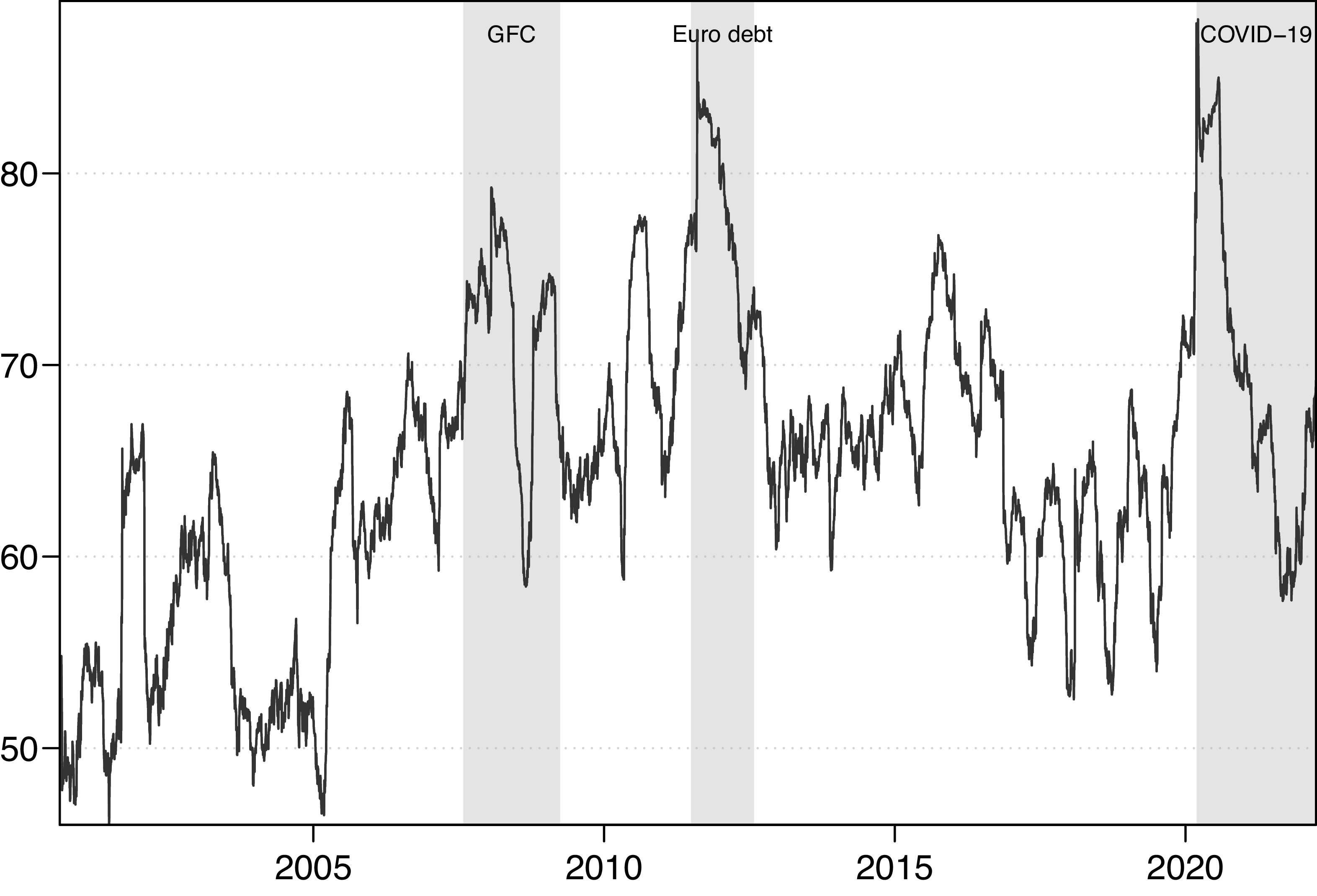
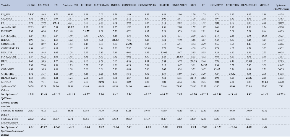


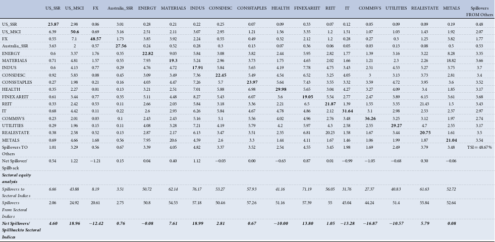
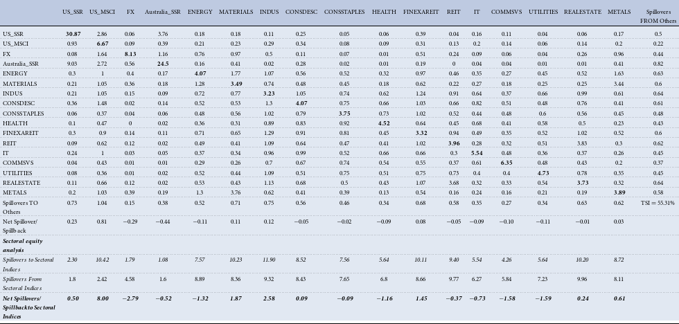
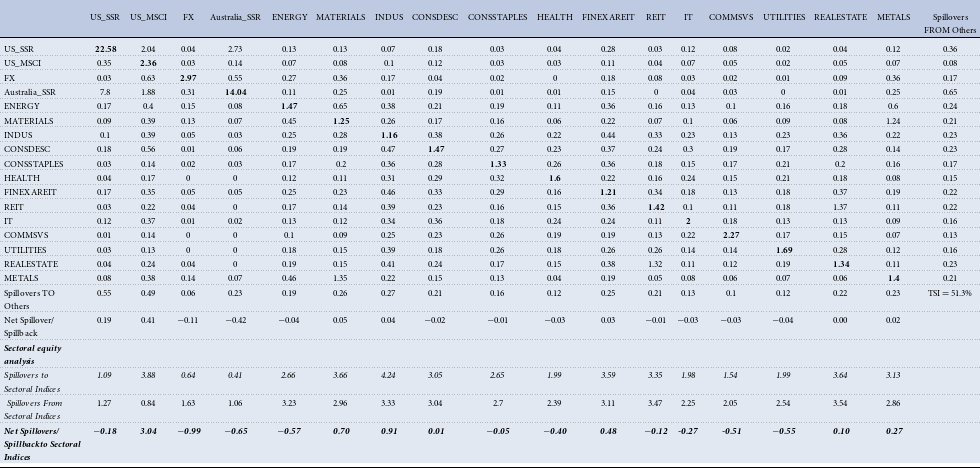


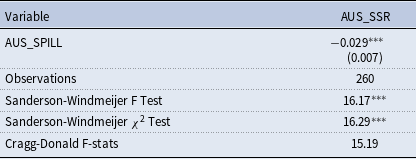


 Open access