


Impact Statement
Turbulence in fluid dynamics is notoriously difficult to model. Data-driven approaches can reduce computational costs but often fail to capture intricate space–time dependencies, leading to rapidly diverging trajectories even in short-term predictions. We propose learning the underlying statistical structure of the flow rather than deterministic trajectories. By first resolving large-scale structure dynamics, we reduce spatial complexity and achieve more stable long-term predictions with an auto-regressive reduced order model (ROM). Finally, we introduce a Gaussian process-based closure strategy to recover small-scale structures.
1. Introduction
When modelling turbulence, the deterministic toolbox encounters two notable challenges. The first relates to the chaotic and unpredictable nature of the dynamical system, which exhibits erratic trajectories seemingly devoid of recurrent patterns and is highly sensitive to initial conditions. As Lorenz famously put it, “The present determines the future, but the approximate present does not approximately determine the future.” The second hurdle arises from the problem’s complex, multi-scale nature. The various scales involved pose difficulties for both DNS, due to the need for excessive constraint on the resolution to account for all the scales, and for machine learning models, which struggle to represent their inherent complexity.
From a reduced-order modeling perspective (with ML strategies being a subcategory of this), we believe that decomposing the task into two consecutive subtasks will overcome both of the aforementioned hurdles. The “first task” would be to derive the dynamics from low-pass filtered data, focusing on the evolution of large structures that contribute significantly to the total kinetic energy. This approach is commonly taken in the fluid mechanics community by relying on Large Eddy Simulations (LES) (see, e.g., Deardorff, Reference Deardorff1970) as opposed to direct numerical simulation (DNS). However, as with LES, the question of closure remains. In the “second task,” therefore, once the trajectories have been reconstructed in the filtered space, we hypothesize the existence of a time-independent and stochastic mapping from that space to the full-resolution domain.
The first task involves constructing an autoregressive and predictive reduced-order model (ROM). The ROM framework has demonstrated promising capabilities across a wide range of dynamical systems, including chaotic ones (Lassila et al., Reference Lassila, Manzoni, Quarteroni, Rozza, Quarteroni and Rozza2014). For instance, proper orthogonal decomposition (POD) enables the projection of a system’s states onto lower-dimensional spaces, which are spanned by the system’s space-time coherent structures referred to as “modes.” As an analytically derived technique, POD uncovers interpretable modes and has been widely adopted as a powerful baseline for dimensionality reduction in physics and turbulence modelling (Schmid, Reference Schmid and Durbin2021). In the nonlinear dynamics community, there has been growing interest in Koopman theory, which supports the existence of linear dynamics even for strongly non-linear systems through the infinite-dimensional Koopman operator (Brunton et al., Reference Brunton, Budišić, Kaiser and Kutz2022). Many works and algorithms focus on finding tractable, finite-dimensional approximations of this operator that capture the essential dynamics. Among these, dynamic mode decomposition (DMD) is one of the most prominent examples (Schmid, Reference Schmid2010). Another powerful approach involves identifying the slowest invariant manifold spanned by the eigenspace of the linearized system near a fixed point and extending it through the system’s nonlinearities. This method, known as spectral submanifolds (SSMs), reveals low-dimensional, non-linear structures that allow for model reduction and simplification of the dynamics (Haller and Ponsioen, Reference Haller and Ponsioen2016). Alternatively, these low-dimensional structures can also be identified using machine learning (ML), thereby relaxing the linear or orthogonality constraints inherent to POD. These ROM approaches can generally be divided into two main categories: Intrusive, which are tailored to the Navier–Stokes equations via, e.g., Galerkin projection (Menier et al., Reference Menier, Bucci, Yagoubi, Mathelin and Schoenauer2023), and non-intrusive, which are purely data-driven (Gupta et al., Reference Gupta, Schmid, Sipp, Sayadi and Rigas2023; Simpson et al., Reference Simpson, Vlachas, Garland, Dervilis and Chatzi2024; Menier et al., Reference Menier, Kaltenbach, Yagoubi, Schoenauer and Koumoutsakos2025; Özalp et al., Reference Özalp, Nóvoa and Magri2025b). Some non-intrusive approaches even operate in a mesh-independent fashion (Serrano et al., Reference Serrano, Migus, Yin, Mazari and Gallinari2023). Recent advances in embedded memory architectures, particularly attention mechanisms and transformers (Vaswani et al., Reference Vaswani, Shazeer, Parmar, Uszkoreit, Jones, Gomez, Kaiser, Polosukhin, Guyon, Luxburg, Bengio, Wallach, Fergus, Vishwanathan and Garnett2017) for time-series applications, have considerably reshaped this landscape (Shokar et al., Reference Shokar, Kerswell and Haynes2024; Solera-Rico et al., Reference Solera-Rico, Sanmiguel Vila, Gómez-López, Wang, Almashjary, Dawson and Vinuesa2024; Zighed et al., Reference Zighed, Nicolas, Gallinari and Sayadi2025).
Regardless of the strategy employed, ROMs typically rely on some form of dimensionality reduction, such as proper orthogonal decomposition (POD), autoencoders, or other compression techniques. This is based on the assumption that the system’s dynamics evolve on a low-dimensional manifold in phase space (Haller and Ponsioen, Reference Haller and Ponsioen2016; Buza et al., Reference Buza, Jain and Haller2021). Remarkably, this assumption often holds for chaotic systems (Liu et al., Reference Liu, Axas and Haller2024), with the infamous Lorenz butterfly serving as a paradigmatic example of such a low-dimensional underlying structure. However, identifying the attractor is not straightforward, and many attempts have shown that, due to inherent turbulence, the resulting models tend to diverge from the true trajectory used in forecast mode (Liu et al., Reference Liu, Axas and Haller2024; Özalp et al., Reference Özalp, N’ovoa and Magri2025a).
Therefore, in this paper, we take a stochastic approach to overcome this challenge. To this end, we use a probabilistic reduction strategy involving an encode-process-decode architecture with a transformer in the latent space and a VAE to generate stochasticity. This enables us to learn the time evolution of the system in the filtered space (i.e., large-scale dynamics) and generate a stochastic ensemble of trajectories whose statistical properties closely resemble those of the filtered flow. A second probabilistic model is then employed to close the dynamics for smaller eddies, generating new samples that are statistically consistent with the true distribution (DNS data) in both time and space. This “closure” is related to the core idea of super-resolution, whereby high-resolution data or fields are reconstructed from coarser measurements or simulations (Dong et al., Reference Dong, Loy, He and Tang2016).
Similar super-resolution approaches have been successfully applied in many different fields, including image processing. (Kim et al., Reference Kim, Lee and Lee2016; Wang et al., Reference Wang, Yu, Wu, Gu, Liu, Dong, Qiao and Loy2018), climate modelling (Jiang et al., Reference Jiang, Yang, Wang, Huang, Xue, Chakraborty, Chen and Qian2023; Soares et al., Reference Soares, Johannsen, Lima, Lemos, Bento and Bushenkova2024), fluid dynamics (Fukami et al., Reference Fukami, Fukagata and Taira2023; Ward, Reference Ward2023), and medical imaging (Huang et al., Reference Huang, Shao and Frangi2017; Chen et al., Reference Chen, Shi, Christodoulou, Xie, Zhou, Li, Frangi, Schnabel, Davatzikos, Alberola-López and Fichtinger2018; Zhang et al., Reference Zhang, Hu, Philbrick, Conte, Sobek, Rouzrokh and Erickson2022), where capturing detailed spatial or temporal patterns is critical for accurate analysis and prediction. For such a small-scale closure, or “super-resolution” task, many studies have utilized groundbreaking advances from the image generation field, such as generative adversarial network (GAN) (De Souza et al., Reference De Souza, Marques, Batagelo and Gois2023) and variational autoencoder (VAE) (Kingma and Welling, Reference Kingma and Welling2013). In the 2020s, denoising diffusion models have emerged as a major breakthrough (Ho et al., Reference Ho, Jain and Abbeel2020; Song and Ermon, Reference Song and Ermon2020). They have enabled state-of-the-art tools for high-resolution image synthesis, although their penetration into physics-based applications remains more limited. Notable examples include diffusion models with embedded transformers. For instance, Serrano et al. (Reference Serrano, Wang, Naour, Vittaut and Gallinari2024), in their AROMA framework, have successfully leveraged this approach to develop a robust and flexible PDE emulator that adapts to different geometries and scales. Mardani et al. (Reference Mardani, Brenowitz, Cohen, Pathak, Chen, Liu, Vahdat, Nabian, Ge, Subramaniam, Kashinath, Kautz and Pritchard2025) integrated a deterministic reduced-order model (ROM) for large-scale dynamics with a diffusion-based closure to improve climatic mesh refinement. Diffusion models, along with the extensive research accompanying them, have demonstrated impressive capabilities in learning complex probability distributions under conditioning; however, they remain computationally expensive both for training and inference (Salimans et al., Reference Salimans, Mensink, Heek and Hoogeboom2024). In this context, we propose an alternative approach for probabilistic closure, leveraging Gaussian Processes to achieve an efficient yet expressive representation of small-scale dynamics.
The paper is organised into three main sections. First, in Section 2, we describe the Kolmogorov flow, the data derived from simulating it, and the filtering strategy. Next, in Section 3, we present the reduced order model (ROM) and its performance on the filtered trajectories. Finally, we introduce the Gaussian process closure and detail its theoretical foundations in Section 4. We also compare its results against other probabilistic baselines whose implementation details are in Appendix A.3. Section 5 presents the entire modeling pipeline with the ROM and the closure combined. Section 6 delivers concluding remarks.
2. Problem formulation
2.1. Kolmogorov flow
The test case considered is the Kolmogorov flow, a two-dimensional, incompressible, unsteady solution of the Navier–Stokes equations with doubly periodic boundary conditions,
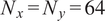
 $ \left[x,y\right]\in {\mathrm{\mathbb{R}}}^2=\left[0,2\pi \right]\times \left[0,2\pi \right] $
. It is driven by a sinusoidal forcing term applied in the
$ \left[x,y\right]\in {\mathrm{\mathbb{R}}}^2=\left[0,2\pi \right]\times \left[0,2\pi \right] $
. It is driven by a sinusoidal forcing term applied in the
 $ x $
-direction. The governing equations are:
$ x $
-direction. The governing equations are:
 $$ {\displaystyle \begin{array}{c}\frac{\partial \mathbf{u}}{\partial t}=-\nabla p-\left(\mathbf{u}\cdot \nabla \right)\mathbf{u}+\frac{1}{\mathit{\operatorname{Re}}}{\nabla}^2\mathbf{u}+\mathbf{f},\\ {}\nabla \cdot \mathbf{u}=0,\\ {}\mathbf{f}\left(x,y\right)=A\sin \left({n}_fy\right)\hskip0.1em {\mathbf{e}}_x\end{array}} $$
where
 $ \mathbf{u}=\left(u,v\right) $
is the velocity field,
$ \mathbf{u}=\left(u,v\right) $
is the velocity field,
 $ p $
the pressure,
$ p $
the pressure,
 $ \nu $
the kinematic viscosity,
$ \nu $
the kinematic viscosity,
 $ \mathit{\operatorname{Re}} $
the Reynolds number and
$ \mathit{\operatorname{Re}} $
the Reynolds number and
 $ \mathbf{f} $
the external forcing. The forcing function
$ \mathbf{f} $
the external forcing. The forcing function
 $ \mathbf{f} $
introduces a steady, spatially periodic body force in the
$ \mathbf{f} $
introduces a steady, spatially periodic body force in the
 $ x $
-direction with wavenumber
$ x $
-direction with wavenumber
 $ {n}_f $
and a fixed amplitude
$ {n}_f $
and a fixed amplitude
 $ A $
.
$ A $
.
This flow, illustrated in Figure 1, is well-suited for investigating fluid instability and the transition to turbulence (Kolmogorov et al., Reference Kolmogorov, Levin, Hunt, Phillips and Williams1991), displaying a variety of regimes depending on the forcing wavenumber
 $ {n}_f $
and Reynolds number
$ {n}_f $
and Reynolds number
 $ \mathit{\operatorname{Re}} $
(Platt et al., Reference Platt, Sirovich and Fitzmaurice1991). For sufficiently high
$ \mathit{\operatorname{Re}} $
(Platt et al., Reference Platt, Sirovich and Fitzmaurice1991). For sufficiently high
 $ \mathit{\operatorname{Re}} $
, an energy cascade is exhibited, whereby large coherent structures decay into smaller eddies that contribute less energy and are eventually dissipated by viscosity. This is the regime of interest in this work. Here, we consider
$ \mathit{\operatorname{Re}} $
, an energy cascade is exhibited, whereby large coherent structures decay into smaller eddies that contribute less energy and are eventually dissipated by viscosity. This is the regime of interest in this work. Here, we consider
 $ \mathit{\operatorname{Re}}=34 $
and forcing wavenumber
$ \mathit{\operatorname{Re}}=34 $
and forcing wavenumber
 $ {n}_f=4 $
, inspired by recent studies from Mo and Magri (Reference Mo and Magri2025) and Racca (Reference Racca2023). These parameters result in a weakly turbulent flow, where different scales interact chaotically together, motivating their study through a statistical lens.
$ {n}_f=4 $
, inspired by recent studies from Mo and Magri (Reference Mo and Magri2025) and Racca (Reference Racca2023). These parameters result in a weakly turbulent flow, where different scales interact chaotically together, motivating their study through a statistical lens.
The simulation is performed on a
 $ 64\times 64 $
Eulerian grid using the publicly available pseudospectral solver kolSol, based on the Fourier–Galerkin approach described by Canuto et al. (Reference Canuto, Quarteroni, Hussaini and Zang2007). We use
$ 64\times 64 $
Eulerian grid using the publicly available pseudospectral solver kolSol, based on the Fourier–Galerkin approach described by Canuto et al. (Reference Canuto, Quarteroni, Hussaini and Zang2007). We use
 $ 32 $
Fourier modes for the resolution. The equations are solved in Fourier space using a fourth-order explicit Runge–Kutta integration scheme with a time step of
$ 32 $
Fourier modes for the resolution. The equations are solved in Fourier space using a fourth-order explicit Runge–Kutta integration scheme with a time step of
 $ \delta t=0.01 $
, and results are stored every
$ \delta t=0.01 $
, and results are stored every
 $ \delta t=0.12 $
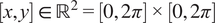
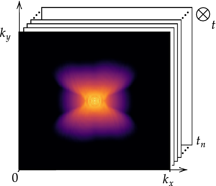
. Velocity fields, shown in Figure 1a, are matrices defined over
$ \delta t=0.12 $
. Velocity fields, shown in Figure 1a, are matrices defined over
 $ {\mathrm{\mathbb{R}}}^{N_x\times {N}_y\times T} $
with
$ {\mathrm{\mathbb{R}}}^{N_x\times {N}_y\times T} $
with
 $ {N}_x={N}_y=64 $
and
$ {N}_x={N}_y=64 $
and
 $ T=1000 $
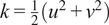
, defining the total number of snapshots. The resulting kinetic energy signal,
$ T=1000 $
, defining the total number of snapshots. The resulting kinetic energy signal,
 $ K $
, is computed by equation (2.2)) and illustrated in Figure 1b.
$ K $
, is computed by equation (2.2)) and illustrated in Figure 1b.
 $$ {k}_t=\frac{1}{2{N}_x{N}_y}\sum \limits_{d=1}^{N_x{N}_y}\left({u}_{d,t}^2+{v}_{d,t}^2\right) $$
Velocity fields and corresponding kinetic energy signal.
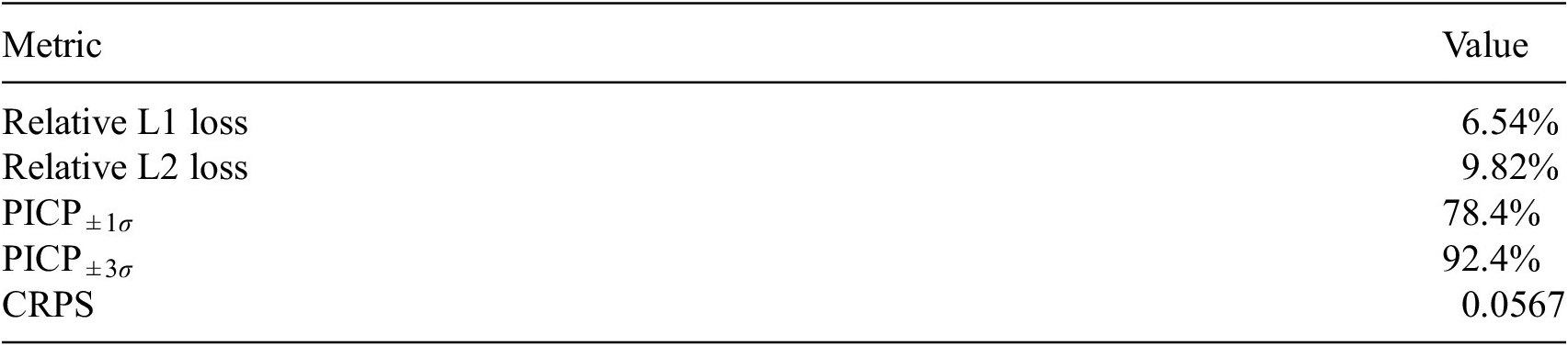
Evaluation metricss of the probabilistic forecasts
The energy cascade, central to Kolmogorov and Richardson’s turbulence theories, is based on decomposing the flow’s energy into structures of different sizes or, equivalently, into different frequencies, also referred to as wavenumbers. Larger structures correspond to lower wavenumbers and typically carry more energy. Our approach relies on separating these scales under the assumption that there exists a dichotomy between large coherent structures and the smaller eddies into which they break down. The spatial distribution of these structures, or more precisely their distribution across wavenumbers, is obtained by applying the two-dimensional (2D) Fourier transform to the field, denoted as:
 $$ U\left(x,y\right)\mapsto \hat{U}\left(m,n\right)={\mathcal{F}}_{2D}\left[U\right]\left(m,n\right) $$
where the transform is defined as:
 $$ \mathcal{F}\left(m,n\right)={\int}_{-\infty}^{\infty }{\int}_{-\infty}^{\infty }U\left(x,y\right)\hskip0.1em {e}^{-j2\pi \left( mx+ ny\right)}\hskip0.1em dx\hskip0.1em dy. $$
Here,
 $ m $
and
$ m $
and
 $ n $
are the spatial frequencies (or wavenumbers) in the
$ n $
are the spatial frequencies (or wavenumbers) in the
 $ x $
- and
$ x $
- and
 $ y $
-directions, respectively. The quantity
$ y $
-directions, respectively. The quantity
 $ \mid \mathcal{F}\left(m,n\right)\mid $
represents the magnitude spectrum of the kinetic energy field
$ \mid \mathcal{F}\left(m,n\right)\mid $
represents the magnitude spectrum of the kinetic energy field
 $ K $
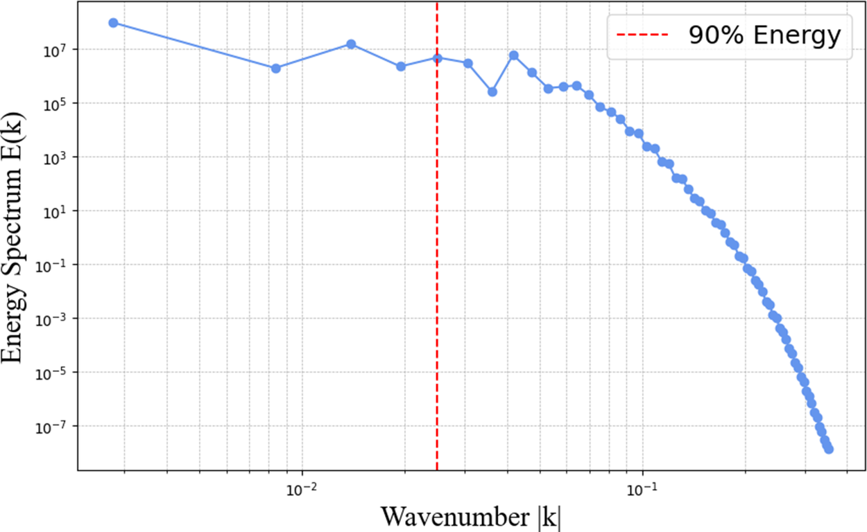
. It provides the distribution of wavenumbers at any given timestep. The time-averaged spectrum is shown in Figure 2 on a logarithmic scale.
$ K $
. It provides the distribution of wavenumbers at any given timestep. The time-averaged spectrum is shown in Figure 2 on a logarithmic scale.
Time-averaged energy spectrum displayed on a logarithmic scale in the wavenumber space.
The spectrogram indicates that the structures with the highest energy are concentrated near the centre, corresponding to small wavenumbers. As the wavenumber increases, moving away from the center, the magnitude generally decreases, reflecting the diminishing contribution of smaller-scale structures to the kinetic energy. Our computed energy cascade is illustrated in Figure 3.
Low-pass filter threshold keeping 90% of the energy.
2.2. Strategy for scale separation
In this work, we propose to classify the flow scales into two families: large and small structures. These two families will be addressed with two distinct strategies. Our goal is to identify an energy threshold in the cascade that retains the larger, “simpler” structures responsible for approximately 90% of the total kinetic energy. This threshold, illustrated Figure 3 corresponds to a critical wavenumber
 $ {k}_c $
, which is then used to construct a low-pass filter
$ {k}_c $
, which is then used to construct a low-pass filter
 $ H $
that separates the large-scale motions from the smaller-scale fluctuations. We emphasise that the filtering operation is intentionally chosen to satisfy scale separation. A filter based on modal compression, such as projection onto a limited number of dominant POD modes, does not selectively remove high-frequency content because these frequencies may still be present in the retained modes.
$ H $
that separates the large-scale motions from the smaller-scale fluctuations. We emphasise that the filtering operation is intentionally chosen to satisfy scale separation. A filter based on modal compression, such as projection onto a limited number of dominant POD modes, does not selectively remove high-frequency content because these frequencies may still be present in the retained modes.
At the low Reynolds number considered here (
 $ \mathit{\operatorname{Re}}=34 $
), the inertial range of the energy spectrum is narrow. The 90% energy threshold was therefore selected as it effectively splits this inertial range, preserving the modes that sustain chaotic dynamics while removing the weakly turbulent fluctuations that decay toward dissipative scales. Applying a slightly more aggressive filter, such as 85%, would eliminate dynamically important modes, including those close to the forcing wavenumber, and would consequently collapse the dynamics onto a deterministic state. For systems studied at higher Reynolds numbers, where the inertial range is significantly broader, the optimal choice of cutoff has been the subject of extensive investigation. In such regimes, it is often found that retaining modes up to
$ \mathit{\operatorname{Re}}=34 $
), the inertial range of the energy spectrum is narrow. The 90% energy threshold was therefore selected as it effectively splits this inertial range, preserving the modes that sustain chaotic dynamics while removing the weakly turbulent fluctuations that decay toward dissipative scales. Applying a slightly more aggressive filter, such as 85%, would eliminate dynamically important modes, including those close to the forcing wavenumber, and would consequently collapse the dynamics onto a deterministic state. For systems studied at higher Reynolds numbers, where the inertial range is significantly broader, the optimal choice of cutoff has been the subject of extensive investigation. In such regimes, it is often found that retaining modes up to
 $ {k}_c\approx 0.2{\eta}^{-1} $
, with
$ {k}_c\approx 0.2{\eta}^{-1} $
, with
 $ \eta $
the Kolmogorov length, is sufficient to ensure stochastic stability (Inubushi et al., Reference Inubushi, Saiki, Kobayashi and Goto2023; Matsumoto et al., Reference Matsumoto, Inubushi and Goto2024).
$ \eta $
the Kolmogorov length, is sufficient to ensure stochastic stability (Inubushi et al., Reference Inubushi, Saiki, Kobayashi and Goto2023; Matsumoto et al., Reference Matsumoto, Inubushi and Goto2024).
 $$ H\left(m,n\right)=\left\{\begin{array}{ll}1,& \mathrm{if}\sqrt{m^2+{n}^2}\le {k}_c,\\ {}0,& \mathrm{otherwise}.\end{array}\right. $$
Applying this filter to the Fourier-transformed field, we obtain the filtered spectrum:
 $$ {\hat{U}}_{\mathrm{low}}\left(m,n\right)=H\left(m,n\right)\cdot \hat{U} $$
Finally, the filtered velocity field
 $ {U}_{\mathrm{low}}\left(x,y\right) $
in physical space, it is recovered by the inverse 2D Fourier transform:
$ {U}_{\mathrm{low}}\left(x,y\right) $
in physical space, it is recovered by the inverse 2D Fourier transform:
 $$ {U}_{\mathrm{low}}\left(x,y\right)={\int}_{-\infty}^{\infty }{\int}_{-\infty}^{\infty }{\hat{U}}_{\mathrm{low}}\left(m,n\right)\hskip0.1em {e}^{j2\pi \left( mx+ ny\right)}\hskip0.1em dm\hskip0.1em dn. $$
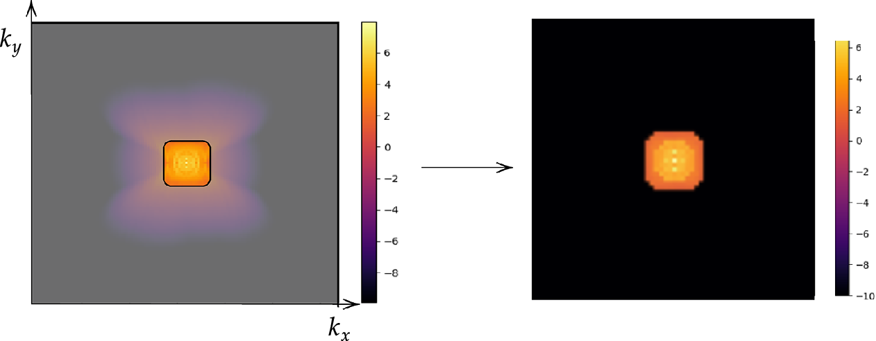
This operation isolates the large-scale structures corresponding to wavenumbers below
 $ {k}_c $
, filtering out the smaller-scale fluctuations as illustrated in Figure 4. While the formulation is presented in a continuous setting, the low-pass filter is implemented in discrete Fourier space using the discrete Fourier transform.
$ {k}_c $
, filtering out the smaller-scale fluctuations as illustrated in Figure 4. While the formulation is presented in a continuous setting, the low-pass filter is implemented in discrete Fourier space using the discrete Fourier transform.
Low-pass filter on the energy spectrum and filtered energy spectrum in the log-scale of the wavenumber space.
The filter reduces the spatial complexity and fine-scale features of the flow that pose challenges for a reduced order model (ROM) to accurately capture (Wang et al., Reference Wang, Akhtar, Borggaard and Iliescu2012; Ahmed et al., Reference Ahmed, Pawar, San, Rasheed, Iliescu and Noack2021). The effects of the filter on the flow is illustrated in Reference Chen, Shi, Christodoulou, Xie, Zhou, Li, Frangi, Schnabel, Davatzikos, Alberola-López and FichtingerFigure 5 with the velocity fields and the kinetic energy represented in Figure 5a,b,c, respectively.
Effect of low-pass filter on velocity fields and kinetic energy.

The filtered kinetic energy is computed from the filtered velocity fields and is not obtained by applying the low-pass filter directly to the kinetic energy field. The filtered velocity fields resulting from this process will be used to train the dynamic reduced-order model (ROM) described in the next section.
3. First task: predicting Filtered dynamics
3.1. Model architecture
We employ a variational autoencoder (VAE) to identify a reduced latent space onto which the dynamics are learned by a transformer, leveraging recent advances in embedded memory and attention mechanisms (Vaswani et al., Reference Vaswani, Shazeer, Parmar, Uszkoreit, Jones, Gomez, Kaiser, Polosukhin, Guyon, Luxburg, Bengio, Wallach, Fergus, Vishwanathan and Garnett2017; Shokar et al., Reference Shokar, Kerswell and Haynes2024). The Mori–Zwanzig formalism and Takens’ theorem (Mori, Reference Mori1965; Zwanzig, Reference Zwanzig1973; Takens, Reference Takens, Rand and Young1981) emphasize the importance of incorporating a memory term to effectively account for the influence of the unobserved, orthogonal subspace on the set of observables learned through the VAE projection. Additionally, Gupta et al. (Reference Gupta, Schmid, Sipp, Sayadi and Rigas2023) demonstrate the limitations of using a purely Markovian representation for rolling out dynamics within a finite, invariant Koopman space. Our architecture, illustrated in Figure 6, is the same as that used in the framework UP-dROM (Zighed et al., Reference Zighed, Nicolas, Gallinari and Sayadi2025).
Reduced-order model architecture, used to predict filtered trajectories.

This model has demonstrated robust performance and generaliaation capabilities in a deterministic setting involving two-dimensional, incompressible flow past a cylinder. The theoretical foundations and implementation details of that ROM are publicly available on GitHub (Zighed, Reference Zighed2025a) and in UP-dROM. Particularly interesting here is the use of a variational autoencoder (VAE), since, apart from its ability to produce a well-structured and dense latent space, which enhances generalisation performance, the VAE learns a distribution over latent variables. This enables the generation of diverse yet physically plausible trajectories. This probabilistic framework, therefore, naturally supports stochastic sampling and uncertainty quantification, as demonstrated in UP-dROM. This compression strategy, therefore, outperforms more classical techniques such as POD. Its advantages stem from its inherently probabilistic formulation, which enables uncertainty quantification and allows us to leverage its variance component, as well as from its increased expressiveness: by relaxing the linearity constraint inherent to POD, the VAE learns a non-linear latent manifold, allowing state-of-the-art compression performance for complex flow dynamics (Zighed et al., Reference Zighed, Nicolas, Gallinari and Sayadi2025).
The VAE learns a mapping
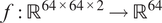 $ f:{\mathrm{\mathbb{R}}}^{64\times 64\times 2}\to {\mathrm{\mathbb{R}}}^{64} $
, and the transformer is trained jointly, leveraging self-attention through two attention blocks to learn the temporal dynamics on this latent manifold. Details of the loss function, the architecture, and hyperparameters are provided in Appendix A.2 (Table A1) along with the algorithm pseudo-code of the training. To provide the model with sufficient prior knowledge of the latent data distribution, we train it using eight flow realizations that share the same statistical properties but differ slightly in their initial conditions. From each realization, only the first 80% of the available 1000 snapshots are used to construct the training and validation datasets, while the remaining 20% are reserved to assess the model’s ability to reproduce long-term statistical behavior. The training–validation split is performed using an odd–even scheme, such that half of the selected snapshots are used for training and the other half for validation. As a result, the training and validation sets each contain 400 snapshots and span the same temporal horizon of 96 nondimensional time units. We denote this time horizon
$ f:{\mathrm{\mathbb{R}}}^{64\times 64\times 2}\to {\mathrm{\mathbb{R}}}^{64} $
, and the transformer is trained jointly, leveraging self-attention through two attention blocks to learn the temporal dynamics on this latent manifold. Details of the loss function, the architecture, and hyperparameters are provided in Appendix A.2 (Table A1) along with the algorithm pseudo-code of the training. To provide the model with sufficient prior knowledge of the latent data distribution, we train it using eight flow realizations that share the same statistical properties but differ slightly in their initial conditions. From each realization, only the first 80% of the available 1000 snapshots are used to construct the training and validation datasets, while the remaining 20% are reserved to assess the model’s ability to reproduce long-term statistical behavior. The training–validation split is performed using an odd–even scheme, such that half of the selected snapshots are used for training and the other half for validation. As a result, the training and validation sets each contain 400 snapshots and span the same temporal horizon of 96 nondimensional time units. We denote this time horizon
 $ \tau $
. The test set extends the validation sequence by an additional 100 snapshots, corresponding to
$ \tau $
. The test set extends the validation sequence by an additional 100 snapshots, corresponding to
 $ 0.25\tau $
, and is used exclusively for long-term evaluation. Once the model generates predictions beyond the
$ 0.25\tau $
, and is used exclusively for long-term evaluation. Once the model generates predictions beyond the
 $ \tau $
mark, we compare the predicted flow statistics with the ground truth statistics to evaluate long-term performance. To keep the presentation clear and succinct, we present results for a single flow instance. The model is tasked with reconstructing the flow from its initial condition and must then roll out the dynamics over an extended prediction horizon, while maintaining statistical consistency with the true flow it aims to emulate. We emphasize that the model could also be evaluated from a more generative perspective, as it is fully capable of generating new flow instances when provided with previously unseen initial conditions. However, we consider this experimental setup to be beyond the scope of the present study.
$ \tau $
mark, we compare the predicted flow statistics with the ground truth statistics to evaluate long-term performance. To keep the presentation clear and succinct, we present results for a single flow instance. The model is tasked with reconstructing the flow from its initial condition and must then roll out the dynamics over an extended prediction horizon, while maintaining statistical consistency with the true flow it aims to emulate. We emphasize that the model could also be evaluated from a more generative perspective, as it is fully capable of generating new flow instances when provided with previously unseen initial conditions. However, we consider this experimental setup to be beyond the scope of the present study.
3.2. Model predictions
After training, the model can predict filtered trajectories based on the filtered initial condition. For each projection, the variational autoencoder (VAE) models a Gaussian distribution over the latent coordinates. The entropy of this distribution, which depends on the variance learned during training, reflects the projection’s likelihood or uncertainty. At each time step, a latent vector is sampled to introduce uncertainty into the prediction. This uncertainty is then propagated through the autoregressive structure of the model. Consequently, each prediction incorporates the accumulated uncertainty from previous steps, as well as the uncertainty introduced by the current stochastic projection. We then decode these latent sample trajectories to project them back to the physical high-dimensional space. These thus constitute a family of plausible trajectories that are consistent with the underlying probability distribution of the flow. We refer to this family as an ensemble, whose mean represents the most probable flow evolution and whose standard deviation represents the uncertainty. As expected, the uncertainty exhibits a growing trend as the dynamical roll-out progresses, as shown in Figure 7. The figure displays the mean trajectory alongside confidence intervals defined by the standard deviation
 $ \sigma $
of the ensemble. We also represent the true validation trajectory to better evaluate the two statistical moments of the generated ensemble.
$ \sigma $
of the ensemble. We also represent the true validation trajectory to better evaluate the two statistical moments of the generated ensemble.
Comparison of predicted and validation trajectories for both flow fields at a given time (
 $ 0.25\tau $
). The plot also shows an ensemble of sampled trajectories generated by the ROM at different locations over
$ 0.25\tau $
). The plot also shows an ensemble of sampled trajectories generated by the ROM at different locations over
 $ 2\tau $
. The solid red line represents the ROM mean prediction, the dashed black line indicates the validation trajectory, and the shaded areas denote the
$ 2\tau $
. The solid red line represents the ROM mean prediction, the dashed black line indicates the validation trajectory, and the shaded areas denote the
 $ \pm \sigma $
and
$ \pm \sigma $
and
 $ \pm 3\sigma $
confidence intervals.
$ \pm 3\sigma $
confidence intervals.

Over time, due to the autoregressive nature of the model, uncertainty tends to accumulate, leading to increasing variance in the predictions. The uncertainties reported in Figure 7 correspond to a total uncertainty that combines both aleatoric and epistemic contributions. Epistemic uncertainty originates from model extrapolation, that is, when inference is performed on input states that are distant from the training distribution. In contrast, aleatoric uncertainty is induced by the intrinsic difficulty of the prediction task and by the irreducible unpredictability of chaotic dynamics. It therefore represents a lower bound on the achievable uncertainty even for inputs drawn from the training distribution. Within the prediction horizon
 $ \tau $
, the validation distribution is effectively identical to the training distribution due to the odd/even train–validation splitting strategy. Nevertheless, a non-zero variance is still observed, which indicates that this uncertainty primarily stems from the aleatoric nature of the task and of the data. As the roll-out progresses in time,
$ \tau $
, the validation distribution is effectively identical to the training distribution due to the odd/even train–validation splitting strategy. Nevertheless, a non-zero variance is still observed, which indicates that this uncertainty primarily stems from the aleatoric nature of the task and of the data. As the roll-out progresses in time,
 $ \left(t>\tau \right) $
the predicted trajectories may progressively depart from the training distribution. In this regime, additional epistemic uncertainty may arise, reflecting the increased model uncertainty associated with out-of-distribution states. Despite this variance, we observe a strong alignment between the predicted mean and the validation trajectory. Furthermore, before the uncertainty amplifies significantly, the confidence interval adapts to the evolving dynamics and transitions. This adaptation effectively balances the interval width with ground truth coverage. This relationship is formally quantified by the Prediction Interval Coverage Probability (PICP), shown in Table 1. The PICP measures the fraction of true values that lie within the predicted confidence intervals, and is given by equation (3.1).
$ \left(t>\tau \right) $
the predicted trajectories may progressively depart from the training distribution. In this regime, additional epistemic uncertainty may arise, reflecting the increased model uncertainty associated with out-of-distribution states. Despite this variance, we observe a strong alignment between the predicted mean and the validation trajectory. Furthermore, before the uncertainty amplifies significantly, the confidence interval adapts to the evolving dynamics and transitions. This adaptation effectively balances the interval width with ground truth coverage. This relationship is formally quantified by the Prediction Interval Coverage Probability (PICP), shown in Table 1. The PICP measures the fraction of true values that lie within the predicted confidence intervals, and is given by equation (3.1).
 $$ \mathrm{PICP}=\frac{1}{N}\sum \limits_{i=1}^N\mathbf{1}\left({y}_i\in \left[{\mu}_i-{\sigma}_i,{\mu}_i+{\sigma}_i\right]\right), $$
where
 $ {\mu}_i $
and
$ {\mu}_i $
and
 $ {\sigma}_i $
are the predicted mean and standard deviation, respectively. The empirical confidence intervals reported in Table 1 fall nearby those expected from a perfect Gaussian distribution, used here solely as theoretical reference values, namely,
$ {\sigma}_i $
are the predicted mean and standard deviation, respectively. The empirical confidence intervals reported in Table 1 fall nearby those expected from a perfect Gaussian distribution, used here solely as theoretical reference values, namely,
 $ 68\% $
within
$ 68\% $
within
 $ \pm \sigma $
and
$ \pm \sigma $
and
 $ 99\% $
within
$ 99\% $
within
 $ \pm 3\sigma $
that indicates that the model finds the mean and variance that distribute the error following a Gaussian-like behavior. The intervals represent a practical trade-off between the ensemble spread and its ability to capture the true values.
$ \pm 3\sigma $
that indicates that the model finds the mean and variance that distribute the error following a Gaussian-like behavior. The intervals represent a practical trade-off between the ensemble spread and its ability to capture the true values.
This trade-off is further quantified by the Continuous Ranked Probability Score (CRPS), also reported in Table 1. CRPS measures the accuracy of a probabilistic forecast; it is given by equation (3.2).
 $$ \mathrm{CRPS}\left(\mu, \sigma; x\right)=\sigma \left[\frac{1}{\sqrt{\pi }}-2\phi \left(\frac{x-\mu }{\sigma}\right)-\frac{x-\mu }{\sigma}\left(2\Phi \left(\frac{x-\mu }{\sigma}\right)-1\right)\right], $$
where
 $ \phi $
and
$ \phi $
and
 $ \Phi $
denote the standard normal probability density function (PDF) and cumulative distribution function (CDF), respectively. Lower CRPS values indicate more accurate probabilistic predictions, penalizing both bias and over or under-confidence in the forecasted uncertainty. The low CRPS value reported here indicates a solid balance between interval conservatism and predictive accuracy. Table 1 also includes the relative
$ \Phi $
denote the standard normal probability density function (PDF) and cumulative distribution function (CDF), respectively. Lower CRPS values indicate more accurate probabilistic predictions, penalizing both bias and over or under-confidence in the forecasted uncertainty. The low CRPS value reported here indicates a solid balance between interval conservatism and predictive accuracy. Table 1 also includes the relative
 $ {\mathrm{\ell}}_1 $
and
$ {\mathrm{\ell}}_1 $
and
 $ {\mathrm{\ell}}_2 $
errors, both highlighting the strong agreement between the ensemble mean and the true trajectories. These metrics are defined in Eq. (3.3)
$ {\mathrm{\ell}}_2 $
errors, both highlighting the strong agreement between the ensemble mean and the true trajectories. These metrics are defined in Eq. (3.3)
 $$ \mathrm{Rel}\hbox{-} \mathrm{L}1=\frac{\sum \mid {y}_{\mathrm{true}}-{y}_{\mathrm{mean}}\mid }{\sum \mid {y}_{\mathrm{true}}\mid}\times 100\%,\hskip1em \mathrm{Rel}\hbox{-} \mathrm{L}2=\frac{\sqrt{\sum {\left({y}_{\mathrm{true}}-{y}_{\mathrm{mean}}\right)}^2}}{\sqrt{\sum {y}_{\mathrm{true}}^2}}\times 100\%. $$
Due to the chaotic nature of the system and the stochasticity inherent in the model, direct pointwise comparisons between individual snapshots and the ground truth are not always meaningful. Furthermore, our aim is to evaluate the prediction horizon beyond the true flow time window. We will therefore assess the model’s long-term validity through statistical consistency. Specifically, we analyse whether the generated trajectory aligns well with the true dynamics in statistical terms, using probability density functions. We compute the probability density functions (PDFs) of the generated filtered velocity fields and compare them to the true filtered PDFs. This frequentist approach ensures that, even if a trajectory deviates in its realization, it is still sampled from the same underlying statistical distribution, and that the long-term dynamical rollout remains consistent with that distribution. Figure 8 illustrates this comparison of the PDFs, showing acceptable statistical agreement.
Probability density functions (PDFs) for fields U and V.

Finally, the Wasserstein distances are computed on the generated data and the true filtered trajectory, which are
 $ 0.0081 $
and
$ 0.0081 $
and
 $ 0.0269 $
for
$ 0.0269 $
for
 $ U $
and
$ U $
and
 $ V $
, respectively. This indicates strong statistical agreement between the generated and reference distributions. This confirms the conclusion that, for both fields
$ V $
, respectively. This indicates strong statistical agreement between the generated and reference distributions. This confirms the conclusion that, for both fields
 $ U $
and
$ U $
and
 $ V $
, even if a particular trajectory deviates from the true one pointwise, or derives from a longer forecast roll-out, it still adheres to the underlying statistical distribution from which the true fields are drawn.
$ V $
, even if a particular trajectory deviates from the true one pointwise, or derives from a longer forecast roll-out, it still adheres to the underlying statistical distribution from which the true fields are drawn.
4. Second task: Gaussian process regression—probabilistic small-scale closure
This second part describes the second identified task of the work: enhancing the fidelity of a reduced-order model acting on filtered flow fields by adopting a Gaussian process regression (GPR) framework. The advantage of Gaussian processes is that exact inference can be performed using matrix operations. It is also worth noting that the hyperparameters controlling the form of the Gaussian process are sparse and can be estimated directly from the data (Williams and Rasmussen, Reference Williams, Rasmussen, Touretzky, Mozer and Hasselmo1995). This results in a lightweight model that enables fast training as well as quasi-real-time closure and inference. The objective is to establish a probabilistic mapping from low-dimensional filtered representations to full-resolution flow fields.
We would like to emphasize that this method can be applied consecutively to virtually any low-fidelity data, whether generated by a machine learning model or numerical simulations such as URANS, or similar. The method introduced in Section 3 is independent of the methodology presented here and merely serves as a necessary underlying dynamical model for low-fidelity data.
4.1. Gaussian process
A Gaussian process (GP) defines a distribution over functions, defined as
 $$ f(x)\sim \mathcal{GP}\left(m(x),\mathcal{K}\left(x,{x}^{\prime}\right)\right), $$
where
 $ m(x) $
is the mean function (typically centred to 0), and
$ m(x) $
is the mean function (typically centred to 0), and
 $ \mathcal{K}\left(x,{x}^{\prime}\right) $
is a positive-definite continuous covariance (kernel) function. Given training data
$ \mathcal{K}\left(x,{x}^{\prime}\right) $
is a positive-definite continuous covariance (kernel) function. Given training data
 $ \mathcal{D}={\left\{\left({x}_i,{y}_i\right)\right\}}_{i=1}^N $
, where
$ \mathcal{D}={\left\{\left({x}_i,{y}_i\right)\right\}}_{i=1}^N $
, where
 $ {y}_i=f\left({x}_i\right)+{\epsilon}_i $
, and
$ {y}_i=f\left({x}_i\right)+{\epsilon}_i $
, and
 $ {\epsilon}_i\sim \mathcal{N}\left(0,{\sigma}_{\epsilon}^2\right) $
, we assume
$ {\epsilon}_i\sim \mathcal{N}\left(0,{\sigma}_{\epsilon}^2\right) $
, we assume
 $ {\overline{y}}_i=0 $
. The true underlying function
$ {\overline{y}}_i=0 $
. The true underlying function
 $ f $
is unknown, and
$ f $
is unknown, and
 $ {\sigma}_{\epsilon}^2 $
is a hyperparameter representing observation noise variance.
$ {\sigma}_{\epsilon}^2 $
is a hyperparameter representing observation noise variance.
Let
 $ X={\left[{x}_1,\dots, {x}_N\right]}^{\top}\in {\mathrm{\mathbb{R}}}^{N\times d} $
be the input matrix, and
$ X={\left[{x}_1,\dots, {x}_N\right]}^{\top}\in {\mathrm{\mathbb{R}}}^{N\times d} $
be the input matrix, and
 $ Y={\left[{y}_1,\dots, {y}_N\right]}^{\top}\in {\mathrm{\mathbb{R}}}^{N\times 1} $
the corresponding output vector. The kernel matrix
$ Y={\left[{y}_1,\dots, {y}_N\right]}^{\top}\in {\mathrm{\mathbb{R}}}^{N\times 1} $
the corresponding output vector. The kernel matrix
 $ {\mathcal{K}}_{XX}\in {\mathrm{\mathbb{R}}}^{N\times N} $
encodes pairwise similarities between training inputs, given
$ {\mathcal{K}}_{XX}\in {\mathrm{\mathbb{R}}}^{N\times N} $
encodes pairwise similarities between training inputs, given
 $$ \mathcal{K}\left({x}_i,{x}_j|\tau \right)={\sigma}^2\exp \left(-\frac{1}{2{l}^2}\parallel {x}_i-{x}_j{\parallel}^2\right), $$
where
 $ \tau =\left\{{\sigma}^2,l\right\} $
are the hyperparameters of the model; the output variance
$ \tau =\left\{{\sigma}^2,l\right\} $
are the hyperparameters of the model; the output variance
 $ {\sigma}^2 $
and the length-scale
$ {\sigma}^2 $
and the length-scale
 $ l $
. The length-scale
$ l $
. The length-scale
 $ l $
controls the smoothness of the function, and the output variance
$ l $
controls the smoothness of the function, and the output variance
 $ {\sigma}^2 $
determines the typical scale of function values. The squared exponential (RBF) kernel is used here due to its smoothness, although for problems exhibiting rougher or periodic behavior, Matérn or periodic kernels might be more appropriate.
$ {\sigma}^2 $
determines the typical scale of function values. The squared exponential (RBF) kernel is used here due to its smoothness, although for problems exhibiting rougher or periodic behavior, Matérn or periodic kernels might be more appropriate.
Let
 $ {\mathcal{D}}^{\ast }={\left\{\left({x}_i^{\ast },{y}_i^{\ast}\right)\right\}}_{i=1}^M $
denote a set of new inputs, with
$ {\mathcal{D}}^{\ast }={\left\{\left({x}_i^{\ast },{y}_i^{\ast}\right)\right\}}_{i=1}^M $
denote a set of new inputs, with
 $ {X}^{\ast }={\left[{x}_1^{\ast },\dots, {x}_M^{\ast}\right]}^{\top}\in {\mathrm{\mathbb{R}}}^{M\times d} $
. The key idea in Gaussian Processes is therefore that the training outputs
$ {X}^{\ast }={\left[{x}_1^{\ast },\dots, {x}_M^{\ast}\right]}^{\top}\in {\mathrm{\mathbb{R}}}^{M\times d} $
. The key idea in Gaussian Processes is therefore that the training outputs
 $ Y $
and the latent function values at test inputs
$ Y $
and the latent function values at test inputs
 $ {f}^{\ast }=f\left({X}^{\ast}\right) $
are jointly distributed as a multivariate Gaussian, as
$ {f}^{\ast }=f\left({X}^{\ast}\right) $
are jointly distributed as a multivariate Gaussian, as
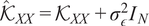
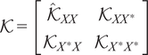
 $$ \left[\begin{array}{c}Y\\ {}{f}^{\ast}\end{array}\right]\sim \mathcal{N}\left(0,\left[\begin{array}{cc}{\hat{\mathcal{K}}}_{XX}& {\mathcal{K}}_{XX^{\ast }}\\ {}{\mathcal{K}}_{X^{\ast }X}& {\mathcal{K}}_{X^{\ast }{X}^{\ast }}\end{array}\right]\right), $$
where
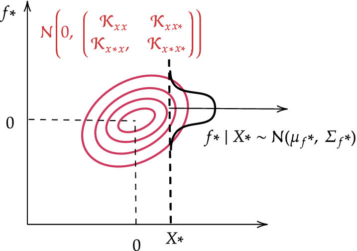
 $ {\hat{\mathcal{K}}}_{XX}={\mathcal{K}}_{XX}+{\sigma}_{\epsilon}^2{I}_N $
includes the observation noise. This means that all data points are partial observations drawn from the same Gaussian.
$ {\hat{\mathcal{K}}}_{XX}={\mathcal{K}}_{XX}+{\sigma}_{\epsilon}^2{I}_N $
includes the observation noise. This means that all data points are partial observations drawn from the same Gaussian.
Given partial observations of a joint Gaussian distribution, it is possible to compute the conditional distribution of unobserved variables, yielding a predictive distribution. The posterior predictive distribution at new inputs
 $ {X}^{\ast } $
is given by the equation (4.3)
$ {X}^{\ast } $
is given by the equation (4.3)
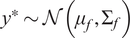
 $$ {f}^{\ast}\mid {X}^{\ast },\mathcal{D}\sim \mathcal{N}\left({\mu}_f,{\Sigma}_f\right), $$
with:
 $$ {\mu}_f={\mathcal{K}}_{X^{\ast }X}{\hat{\mathcal{K}}}_{XX}^{-1}Y,\hskip1em {\Sigma}_f={\mathcal{K}}_{X^{\ast }{X}^{\ast }}-{\mathcal{K}}_{X^{\ast }X}{\hat{\mathcal{K}}}_{XX}^{-1}{\mathcal{K}}_{XX^{\ast }}. $$
Figure 9 illustrates a 2D example where
 $ N=M=1 $
.
$ N=M=1 $
.
Gaussian process prediction example for a single training and inference point (
 $ N=M=1 $
).
$ N=M=1 $
).
The hyperparameters
 $ \tau $
and
$ \tau $
and
 $ {\sigma}_{\epsilon } $
are optimized by maximizing the log-marginal likelihood of the training outputs
$ {\sigma}_{\epsilon } $
are optimized by maximizing the log-marginal likelihood of the training outputs
 $ Y $
given inputs
$ Y $
given inputs
 $ X $
, with the equation (4.4)
$ X $
, with the equation (4.4)
 $$ \log p\left(Y|X,{\sigma}_{\epsilon}^2,\tau \right)=\log \left[\int p\left(Y|\tilde{f},{\sigma}_{\epsilon}^2\right)p\Big(\tilde{f}|X,\tau \Big)d\tilde{f}\right] $$
 $$ \log p\left(Y|X\right)=\log \left[\int \mathcal{N}\left(Y|\tilde{f},{\sigma}_{\epsilon}^2I\right).\mathcal{N}\Big(\tilde{f}|0,{\mathcal{K}}_{xx}\Big)d\tilde{f}\right] $$
 $$ \log p\left(Y|X\right)=\log \mathcal{N}\left(Y|0,{\hat{\mathcal{K}}}_{XX}\right) $$
where
 $$ {\displaystyle \begin{array}{c}{\hat{\mathcal{K}}}_{XX}={\mathcal{K}}_{XX}+{\sigma}_{\epsilon}^2I\\ {}\log p\left(Y|X\right)=-\frac{1}{2}{Y}^{\top }{\hat{\mathcal{K}}}_{XX}^{-1}Y-\frac{1}{2}\log \left|{\hat{\mathcal{K}}}_{XX}\right|-\frac{N}{2}\log \left(2\pi \right)\end{array}} $$
This training process is summarized in Algorithm 1.
Algorithm 1 Gaussian Process Hyperparameter Training
1: Input: Training dataset
 $ \mathcal{D}={\left\{\left({x}_i,{y}_i\right)\right\}}_{i=1}^N $
2: initialise hyperparameters
 $ \tau $
,
$ \tau $
,
 $ {\sigma}_{\epsilon}^2 $
3: while log-likelihood:
 $ \log p\left(Y|X,\tau, {\sigma}_{\epsilon}^2\right) $
not maximized do
$ \log p\left(Y|X,\tau, {\sigma}_{\epsilon}^2\right) $
not maximized do
4: Compute covariance matrix
 $ {\hat{\mathcal{K}}}_{XX} $
5: Compute log-likelihood:
 $ \log p\left(Y|X,\tau, {\sigma}_{\epsilon}^2\right) $
6: Update hyperparameters
 $ \tau $
,
$ \tau $
,
 $ {\sigma}_{\epsilon}^2 $
7: end while
At inference time, the predictive distribution for a new point
 $ {x}^{\ast } $
is computed as shown in Algorithm 2.
$ {x}^{\ast } $
is computed as shown in Algorithm 2.
Algorithm 2 Gaussian Process Inference
1: Input: Training data
 $ \mathcal{D}={\left\{\left({x}_i,{y}_i\right)\right\}}_{i=1}^N $
, new samples input
$ \mathcal{D}={\left\{\left({x}_i,{y}_i\right)\right\}}_{i=1}^N $
, new samples input
 $ {x}^{\ast } $
, and trained hyperparameters
$ {x}^{\ast } $
, and trained hyperparameters
 $ \tau $
2: Compute kernel submatrices:
 $ \mathcal{K}=\left[\begin{array}{cc}{\hat{\mathcal{K}}}_{XX}& {\mathcal{K}}_{XX^{\ast }}\\ {}{\mathcal{K}}_{X^{\ast }X}& {\mathcal{K}}_{X^{\ast }{X}^{\ast }}\end{array}\right] $
3: Compute posterior mean and variance:
 $ {\mu}_f={\mathcal{K}}_{X^{\ast }X}{\hat{\mathcal{K}}}_{XX}^{-1}Y,\hskip1em {\Sigma}_f={\mathcal{K}}_{X^{\ast }{X}^{\ast }}-{\mathcal{K}}_{X^{\ast }X}{\hat{\mathcal{K}}}_{XX}^{-1}{\mathcal{K}}_{XX^{\ast }} $
4: Predict output: sample
 $ {y}^{\ast}\sim \mathcal{N}\left({\mu}_f,{\Sigma}_f\right) $
4.2. GPR applied for closure
Rather than finding a mapping in physical space, which would result in too many degrees of freedom, we exploit the data’s inherent low-dimensional structure and extract the mapping in a reduced space constructed using proper orthogonal decomposition (POD). POD is a data-driven, linear reduction technique that extracts the dominant coherent structures from the system. We apply POD to the snapshot matrix
 $ \varphi \in {\mathrm{\mathbb{R}}}^{T\times D} $
, where each column of
$ \varphi \in {\mathrm{\mathbb{R}}}^{T\times D} $
, where each column of
 $ \varphi $
represents the D-dimensional system state at a given time. Using Singular Value Decomposition (SVD), we write :
$ \varphi $
represents the D-dimensional system state at a given time. Using Singular Value Decomposition (SVD), we write :
 $$ \varphi =U\Sigma {V}^T $$
where
 $ U\in {\mathrm{\mathbb{R}}}^{D\times r} $
contains the spatial modes,
$ U\in {\mathrm{\mathbb{R}}}^{D\times r} $
contains the spatial modes,
 $ \Sigma \in {\mathrm{\mathbb{R}}}^{r\times r} $
is the diagonal matrix of singular values, and
$ \Sigma \in {\mathrm{\mathbb{R}}}^{r\times r} $
is the diagonal matrix of singular values, and
 $ V\in {\mathrm{\mathbb{R}}}^{T\times r} $
holds the latent coordinates, with
$ V\in {\mathrm{\mathbb{R}}}^{T\times r} $
holds the latent coordinates, with
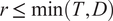 $ r\le \min \left(T,D\right) $
. We define
$ r\le \min \left(T,D\right) $
. We define
 $ \Psi =U\Sigma $
, which combines the spatial structures with their energetic weights. A truncation at rank
$ \Psi =U\Sigma $
, which combines the spatial structures with their energetic weights. A truncation at rank
 $ r=3 $
is performed, since these encapsulate 98% of the total energy in both the filtered and full-scale datasets. Better results could arguably be achieved by considering more modes, albeit at a higher training cost, without modifying the implementation. We assume an invariant reduced basis
$ r=3 $
is performed, since these encapsulate 98% of the total energy in both the filtered and full-scale datasets. Better results could arguably be achieved by considering more modes, albeit at a higher training cost, without modifying the implementation. We assume an invariant reduced basis
 $ U $
, in order to enforce modal and statistical consistency throughout long dynamical roll-outs. Finally, we use the symbol,
$ U $
, in order to enforce modal and statistical consistency throughout long dynamical roll-outs. Finally, we use the symbol,
 $ {}^{\wedge } $
, to indicate filtered data, while full-scale data is presented without any symbol. Figure 10 illustrates the mapping performed by the Gaussian Process Regression (GPR).
$ {}^{\wedge } $
, to indicate filtered data, while full-scale data is presented without any symbol. Figure 10 illustrates the mapping performed by the Gaussian Process Regression (GPR).
Mapping between low-pass filtered POD space and full-scale POD space.

Therefore, the system’s state at time t can be approximated by a combination of the three identified POD modes, with
 $$ \hat{\varphi}\approx {\hat{\alpha}\hat{\psi}}_1+{\hat{\beta}\hat{\psi}}_2+{\hat{\gamma}\hat{\psi}}_3, $$
for the filtered and, with
 $$ \varphi \approx {\alpha \psi}_1+{\beta \psi}_2+{\gamma \psi}_3, $$
for the full-state data, respectively. We therefore aim to learn a time independent mapping, such that :
 $$ f:\left(\hat{\alpha},\hat{\beta},\hat{\gamma}\right)\mapsto \left(\alpha, \beta, \gamma \right). $$
Rather than learning a deterministic function, we place a prior over
 $ f $
:
$ f $
:
 $$ f\sim \mathcal{GP}\left(0,\mathcal{K}\right). $$
As a result, given the training data
 $ \mathcal{D} $
, we infer a posterior over functions
$ \mathcal{D} $
, we infer a posterior over functions
 $$ p\left(f|\mathcal{D},\hat{\alpha},\hat{\beta},\hat{\gamma}\right). $$
The key advantage of Gaussian process regression (GPR) over classical regression methods is its inherently probabilistic formulation. By sampling from the predictive distribution
 $ {y}^{\ast}\sim {f}^{\ast } $
, GPR produces an ensemble of outputs whose statistical properties are consistent with the underlying distribution of the flow. The associated variance naturally quantifies model confidence, providing not only pointwise predictions, but also credible intervals around them. This uncertainty-aware modelling approach aligns with recent turbulence modelling developments, which increasingly focus on learning statistical representations of flows rather than deterministic trajectories. It also aligns with the objective of this work, which is to remain within a statistical framework for reconstruction.
$ {y}^{\ast}\sim {f}^{\ast } $
, GPR produces an ensemble of outputs whose statistical properties are consistent with the underlying distribution of the flow. The associated variance naturally quantifies model confidence, providing not only pointwise predictions, but also credible intervals around them. This uncertainty-aware modelling approach aligns with recent turbulence modelling developments, which increasingly focus on learning statistical representations of flows rather than deterministic trajectories. It also aligns with the objective of this work, which is to remain within a statistical framework for reconstruction.
The Gaussian Process is trained and evaluated on the portion
 $ \tau $
of the DNS trajectory, using an 85/15 sequential split. Unlike the ROM, which employs an odd–even snapshot partition, the GP uses a contiguous, time-ordered split. This results in a training and evaluation dataset comprising 680 snapshots and 120 snapshots, respectively. Using such a limited training set is sufficient given the very limited number of trainable hyperparameters. More importantly, classical GPs scale poorly with the number of training samples: training requires the inversion (or Cholesky factorization) of the kernel similarity matrix
$ \tau $
of the DNS trajectory, using an 85/15 sequential split. Unlike the ROM, which employs an odd–even snapshot partition, the GP uses a contiguous, time-ordered split. This results in a training and evaluation dataset comprising 680 snapshots and 120 snapshots, respectively. Using such a limited training set is sufficient given the very limited number of trainable hyperparameters. More importantly, classical GPs scale poorly with the number of training samples: training requires the inversion (or Cholesky factorization) of the kernel similarity matrix
 $ \mathbf{K}\in {\mathrm{\mathbb{R}}}^{m\times m} $
, with
$ \mathbf{K}\in {\mathrm{\mathbb{R}}}^{m\times m} $
, with
 $ m $
the number of samples, leading to a computational cost of
$ m $
the number of samples, leading to a computational cost of
 $ \mathcal{O}\left({m}^3\right) $
. As a result, increasing
$ \mathcal{O}\left({m}^3\right) $
. As a result, increasing
 $ m $
rapidly becomes computationally prohibitive. Furthermore, in high-dimensional settings, overly large training sets may degrade kernel quality due to collapsing pairwise similarities. For these reasons, GPs are commonly trained on carefully selected representative subsets, with scalability addressed through retraining, downsampling, or feature selection such as Automatic Relevance Determination (ARD). Figure 11 illustrates such Gaussian Process regression in our experimental set-up.
$ m $
rapidly becomes computationally prohibitive. Furthermore, in high-dimensional settings, overly large training sets may degrade kernel quality due to collapsing pairwise similarities. For these reasons, GPs are commonly trained on carefully selected representative subsets, with scalability addressed through retraining, downsampling, or feature selection such as Automatic Relevance Determination (ARD). Figure 11 illustrates such Gaussian Process regression in our experimental set-up.
Figure 11a shows the Gaussian process regression of the three reduced manifold variables in both the training and validation sets. These three coefficients define a trajectory that evolves on a latent manifold embedded in the three-dimensional space spanned by the first three POD modes, as illustrated in Figure 11b.
Gaussian Process Regression (GPR) train and validation over 3 POD coefficients.

The model performance is evaluated after the reverse projection to the high-dimensional input space, using several metrics that quantify the accuracy of predictions and the quality of uncertainty estimates on the validation set. We use the relative L1 error, the relative L2 error, and the PICP introduced in Section 3.2 for a Confidence Interval (CI) of
 $ \pm \sigma $
and
$ \pm \sigma $
and
 $ \pm 3\sigma $
and the CRPS. They are documented in Table 2.
$ \pm 3\sigma $
and the CRPS. They are documented in Table 2.
Evaluation metrics on validation set
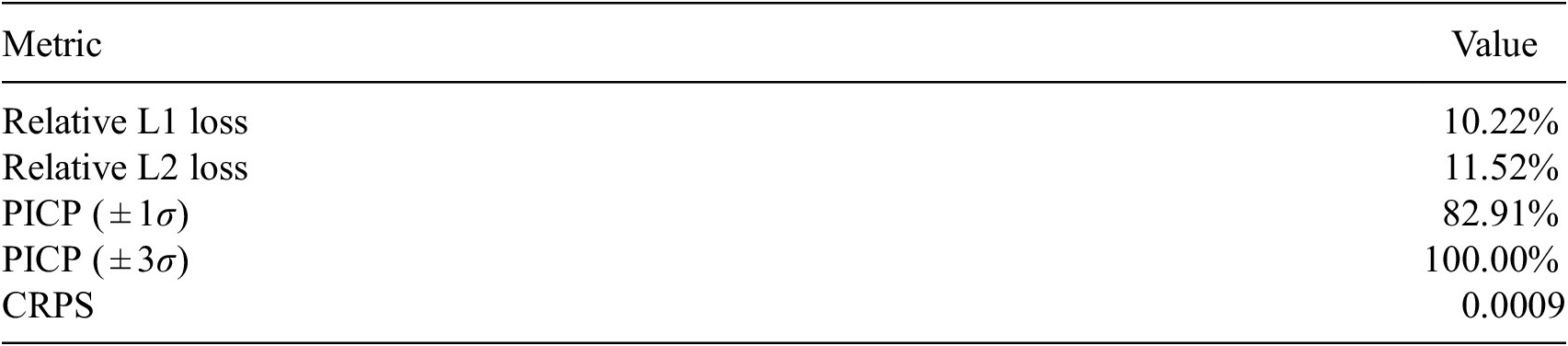
The performance of the Gaussian Process suggests that it acquired strong prior knowledge during training, enabling it to make meaningful predictions with reliable confidence intervals. The first-moment scores are slightly above 10% on the validation set, which indicates a decent level of fidelity to the data. The Prediction Interval Coverage Probability (PICP) reaches 82%, using intervals constructed at one standard deviation. The low Continuous Ranked Probability Score (CRPS) indicates that this coverage is achieved while maintaining minimal interval width. Following training, the model has identified the optimal set of three hyperparameters,
 $ {\sigma}^2 $
,
$ {\sigma}^2 $
,
 $ l $
, and
$ l $
, and
 $ {\sigma}_{\epsilon}^2 $
, which enables the construction of the similarity kernel shown in Figure 12. This consequently allows inference on unseen data. The mapping can be instantaneously sampled from the GP as new data arrives, allowing for real-time closure.
$ {\sigma}_{\epsilon}^2 $
, which enables the construction of the similarity kernel shown in Figure 12. This consequently allows inference on unseen data. The mapping can be instantaneously sampled from the GP as new data arrives, allowing for real-time closure.
Training samples kernel
 $ {\mathcal{K}}_{XX} $
.
$ {\mathcal{K}}_{XX} $
.

The structure of the similarity kernel suggests that the snapshots are highly correlated with one another, even when they are temporally distant. This strong correlation indicates promising potential for generalization to unseen data.
5. Full model prediction
As illustrated in the previous section, the Gaussian Processes are trained to map filtered data to full-scale Direct Numerical Simulation (DNS) data.
Initially trained on true filtered trajectories, the Gaussian process, when applied in the full model format, predicts full-scale data from the filtered trajectories generated by the dynamical reduced-order model (ROM) during inference. This establishes an end-to-end data pipeline where the input is the filtered initial condition and the output is the generated full-scale trajectories, as illustrated in Figure 13.
Data pipeline.

When we condition the Gaussian Process (GP) model on new, unobserved inference data
 $ {X}^{\ast } $
, which is generated by the Reduced Order Model (ROM), we obtain the posterior distribution:
$ {X}^{\ast } $
, which is generated by the Reduced Order Model (ROM), we obtain the posterior distribution:
 $$ {f}^{\ast}\sim \mathcal{GP}\left({\mu}_f,{\mathcal{K}}_{XX^{\ast }}\right), $$
where
 $ {\mu}_f $
denotes the posterior mean, and
$ {\mu}_f $
denotes the posterior mean, and
 $ {\mathcal{K}}_{XX^{\ast }} $
represents the updated covariance matrix. This matrix captures the similarity between the training data
$ {\mathcal{K}}_{XX^{\ast }} $
represents the updated covariance matrix. This matrix captures the similarity between the training data
 $ X $
and the inference points
$ X $
and the inference points
 $ {X}^{\ast } $
. From this posterior, we can draw samples
$ {X}^{\ast } $
. From this posterior, we can draw samples
 $ {f}^{\ast } $
, which represent the predicted full-scale mode coefficients. These coefficients are treated by the GPR as independent samples from a joint distribution; this step is therefore entirely time-independent. The generated output successfully reconstructs filtered out frequencies, as illustrated by the averaged spectrograms before and after the application of the Gaussian Process. Figure 14 shows these spectrograms for the kinetic energy.
$ {f}^{\ast } $
, which represent the predicted full-scale mode coefficients. These coefficients are treated by the GPR as independent samples from a joint distribution; this step is therefore entirely time-independent. The generated output successfully reconstructs filtered out frequencies, as illustrated by the averaged spectrograms before and after the application of the Gaussian Process. Figure 14 shows these spectrograms for the kinetic energy.
Averaged energy spectrograms in the wavenumber space.

The combination of the reduced order model (ROM) and the Gaussian process (GP) enables the generation of new trajectories that, while potentially deviating from the ground truth, remain statistically consistent with the underlying dynamics. At any given snapshot in time, the GP is capable of reconstructing missing or unresolved flow structures, such as small-scale eddies, as illustrated in Figure 15.
Energy at a snapshot T = 120.

It is evident that one-to-one image comparisons with flows such as those shown in Figure 15a,c appear different. Beyond a certain prediction horizon, pixel-to-pixel comparisons become irrelevant, since our framework does not simply learn and reproduce specific trajectories. Instead, it learns the underlying statistics of the flow and should not be expected to reconstruct identical realizations.
5.1. Evaluation on long term predictions
To assess the stability of the proposed framework over long prediction horizons, we evaluate whether the statistical properties of the generated flow are preserved in time. Specifically, we compare the probability density functions (PDFs) of the predicted full-scale flow with those obtained from the test dataset.
The training and validation datasets span a temporal horizon of 96 nondimensional time units, which we denote by
 $ \tau $
. The test dataset covers a longer horizon of
$ \tau $
. The test dataset covers a longer horizon of
 $ 1.25\hskip0.1em \tau $
, while the ROM+GP framework is used to generate trajectories extending up to
$ 1.25\hskip0.1em \tau $
, while the ROM+GP framework is used to generate trajectories extending up to
 $ 4\hskip0.1em \tau $
. Figure 16 shows the kinetic energy rollout
$ 4\hskip0.1em \tau $
. Figure 16 shows the kinetic energy rollout
 $ k $
computed on a two-dimensional grid and reduced to a one-dimensional signal by averaging along the
$ k $
computed on a two-dimensional grid and reduced to a one-dimensional signal by averaging along the
 $ x $
-direction. The predicted energy PDFs are evaluated over successive temporal windows of length
$ x $
-direction. The predicted energy PDFs are evaluated over successive temporal windows of length
 $ \tau $
and compared against the reference PDF computed from the test dataset. Figure 16 also reports the kinetic energy density obtained before applying the Gaussian process closure.
$ \tau $
and compared against the reference PDF computed from the test dataset. Figure 16 also reports the kinetic energy density obtained before applying the Gaussian process closure.
Space-time evolution of the kinetic energy
 $ k=\frac{1}{2}\left({u}^2+{v}^2\right) $
averaged along the
$ k=\frac{1}{2}\left({u}^2+{v}^2\right) $
averaged along the
 $ x $
-direction. The color scale represents
$ x $
-direction. The color scale represents
 $ {\left\langle k\left(y,t\right)\right\rangle}_x $
as a function of the wall-normal coordinate
$ {\left\langle k\left(y,t\right)\right\rangle}_x $
as a function of the wall-normal coordinate
 $ y $
and the dimensionless time. The data distribution for each
$ y $
and the dimensionless time. The data distribution for each
 $ \tau $
interval is compared with the PDF of the test set.
$ \tau $
interval is compared with the PDF of the test set.

We observe that even when predicting over a time horizon four times longer than the training/evaluation window, the closure fixes the filtered rollout energy statistics and preserves them in forecast mode without significant drift. This is supported by Figure 17 and to quantify this observation, we compute in Figure 17a the Wasserstein distance between the predicted energy density and the test set distribution, using windows of
 $ 0.5\tau $
.
$ 0.5\tau $
.
Statistical consistency of long roll-outs, quantified by the Wasserstein distance of energy distributions and the preservation of chaotic dynamics.

The results highlighted by Figure 17a demonstrate that the statistical properties of the flow remain stable throughout the forecasting window. Despite evolving over a time horizon significantly longer than the training window, the model maintains both spatial and temporal complexity without substantial statistical degradation while preserving the chaotic nature of the dynamics. Figure 17b illustrates that the dynamics are sustained upon a chaotic attractor represented in the delay embedding space of the dissipation signal, where
 $ \Delta t $
values 2 snapshots. The dissipation is computed as
$ \Delta t $
values 2 snapshots. The dissipation is computed as
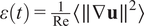 $ \varepsilon (t)=\frac{1}{\operatorname{Re}}\left\langle \parallel \nabla \mathbf{u}{\parallel}^2\right\rangle $
averaged over the domain.
$ \varepsilon (t)=\frac{1}{\operatorname{Re}}\left\langle \parallel \nabla \mathbf{u}{\parallel}^2\right\rangle $
averaged over the domain.
From a dynamical perspective, the long-term forecast also remains consistent with the expected behavior of the numerically simulated Kolmogorov flow as supported by Figure 18. Figure 18a compares the turbulent kinetic energy (TKE) spectrograms obtained from the direct numerical simulation (DNS) and from the long roll-out of the generated flow. A good agreement is observed between the two spectra, in particular in the inertial range, which is nearly identical in both cases.
Comparison of turbulent energy spectra and dissipative manifolds for reduced bases of 3 and 18 POD modes.

Figure 18a also shows that the generated flow nevertheless exhibits a slightly more dissipative behavior. This discrepancy, however, remains moderate. Taking into account the dimensional reduction performed to attain the closure explains the origin of this discrepancy. The closure is applied after projecting the dynamics onto the first three POD modes. Although these modes capture nearly all of the system energy, the small number of retained modes, together with the linear nature of the projection, truncates modes associated with potentially high-wavenumber structures. Figure 18a additionally shows that this truncation reproduces exactly the loss of wavenumbers observed after our model’s reconstruction. This indicates that the additional dissipation observed in the reconstructed flow is not attributable to the filtering strategy, the ROM, or the closure mechanism itself, but rather to the choice of the reduced basis onto which the closure is applied.
Figure 18b illustrates the two-dimensional dissipative manifold obtained from the ROM+GP procedure when the closure is performed using three POD modes. The manifold is constructed using delay embeddings of the dissipation signal with
 $ \Delta t=4 $
, while the reference attractor is generated using the same embedding applied to the ensemble of true (DNS) trajectories. For visualization purposes, a moving-average smoothing filter with a sliding window of 20 snapshots is applied to the manifold corresponding to the generated trajectory. Although the global structure and topology remain consistent with those of the turbulent attractor, the dissipative shift becomes more apparent.
$ \Delta t=4 $
, while the reference attractor is generated using the same embedding applied to the ensemble of true (DNS) trajectories. For visualization purposes, a moving-average smoothing filter with a sliding window of 20 snapshots is applied to the manifold corresponding to the generated trajectory. Although the global structure and topology remain consistent with those of the turbulent attractor, the dissipative shift becomes more apparent.
Figure 18c and 18d show that increasing the number of POD modes from 3 to 18 corrects both the turbulent energy spectrogram and the associated dissipative manifold of the generated flow. This improvement is achieved at the expense of a higher computational cost and a degradation of first-moment accuracy (with
 $ {L}_1 $
and
$ {L}_1 $
and
 $ {L}_2 $
errors of
$ {L}_2 $
errors of
 $ 73.6\% $
and
$ 73.6\% $
and
 $ 75.5\% $
, respectively). The second-moment accuracy, however, remains satisfactory, with
$ 75.5\% $
, respectively). The second-moment accuracy, however, remains satisfactory, with
 $ {PICP}_{\pm 3\sigma }=87.7\% $
. Although first-moment errors are not the primary objective, retaining only three POD modes emerges as a suitable compromise between reconstruction capability and statistical and dynamical consistency.
$ {PICP}_{\pm 3\sigma }=87.7\% $
. Although first-moment errors are not the primary objective, retaining only three POD modes emerges as a suitable compromise between reconstruction capability and statistical and dynamical consistency.
5.2. Comparison to alternative ML architectures
We compare the performance of our GPR-based model against state-of-the-art probabilistic machine learning predictors, namely the variational autoencoder (VAE) and diffusion models. This choice is motivated by the remarkable capabilities of these statistical distribution emulators, particularly in image generation and hyper-resolution tasks. In this context the multi-scale closure task is performed using these ML architectures. Appendix A.3 provides the implementation details for each architecture, along with further justification for their selection as benchmarks.
The results for both the VAE and the diffusion model are summarized over the validation set in Table 3. Both were trained on the same flow resolution as the GP and with identical train and validation sets. All performance measurements were obtained on a workstation equipped with an NVIDIA RTX 4000 Ada Generation GPU, which was used for training the VAE and diffusion models. Gaussian process regression was trained on a 13th Gen Intel i9-13950HX CPU (2.20 GHz).
Comparison of evaluation metrics between the our Gaussian Process Regression, the Variational Autoencoder (VAE), and diffusion model

The Gaussian process outperforms these two baselines for both the first and second moment metrics on validation set. It should be noted, however, that although the diffusion model demonstrates state-of-the-art performance in image generation and does not rely on any prior assumptions about the data structure, its training and inference costs are notably high. Specifically, generating a single image requires numerous denoising steps (1000 in our implementation), meaning the model must perform a thousand inference passes to produce a unique sample. This results in a significant computational expense. We hypothesise that, with a larger model and a more exhaustive search for optimal hyperparameters, diffusion could perform better than shown here, especially with access to more data. However, such a search would incur prohibitive computational costs. The VAE needs to perform inference once per sample, resulting in faster predictions but potentially high computational cost, especially with deeper encoders and decoders. The GP, in contrast, generates all samples at once, directly in the reduced manifold space by treating different snapshots as partial observations of a single underlying Gaussian distribution. Notably, only three hyperparametrs per GP were optimized during training. Since we predict a three-dimensional modal state, we train one GP for each output dimension. This results in a total of three GPs and nine optimized hyperparametrs overall, yielding a considerably more efficient and interpretable model.
6. Conclusion
This study introduces a predictive modeling framework for the long-term generation and forecasting of chaotic trajectories representative of turbulent regimes. The proposed approach adopts a fully stochastic formulation that exploits scale separation to reproduce the statistical properties of the original system. In this framework, the coherent large-scale dynamics, identified through data filtering, are first predicted, while the influence of small scale fluctuations is incorporated through a stochastic representation. This simplification enables the reduced-order model (ROM) to focus on the evolution of time-dependent dynamics rather than the detailed reconstruction of fine-scale features. Once the filtered trajectories are inferred, a secondary, time-independent model probabilistically maps these results back to the full-scale space. Notably, the two models operate independently and are designed to be modular: the ROM can emulate large-scale dynamics while being coupled with alternative closure schemes, and the small-scale learning strategy can serve as a closure mechanism for alternative low-fidelity dynamical models. This modular architecture is designed to provide flexibility and adaptability for applications exhibiting scale separation.
The reduced-order model (ROM) used in this framework is based on our recent work, UPdROM (Zighed et al., Reference Zighed, Nicolas, Gallinari and Sayadi2025). Although it was originally trained and validated on the deterministic flow past a blunt object, the model’s stochastic nature enables it to generate ensembles of trajectories whose statistics closely align with the Kolmogorov flow distribution. This distribution is considered here as a benchmark validation case. The model learns a probabilistic mapping to a low-dimensional manifold using a variational autoencoder (VAE). Dynamics within this latent space are captured by a transformer architecture. Furthermore, by sampling stochastically from the VAE at each time step, the model generates ensembles of trajectories. The ensemble mean remains faithful to the true data, while the variance demonstrates strong coverage properties, as confirmed by the prediction interval coverage probability (PICP). The trade-off between ensemble spread and coverage is quantified by a Continuous Ranked Probability Score (CRPS) approaching zero. To close the spatial structures, we use a Gaussian process (GP) to map from the filtered space to the full-scale space within their respective POD subspaces. Using only three POD modes, we can faithfully reconstruct the multi-scale data, as demonstrated by strong test-set performance. This includes accurate first-moment statistics (with low
 $ {\mathrm{\ell}}_1 $
and
$ {\mathrm{\ell}}_1 $
and
 $ {\mathrm{\ell}}_2 $
errors) and robust second-moment statistics (as evidenced by the PICP and CRPS).
$ {\mathrm{\ell}}_2 $
errors) and robust second-moment statistics (as evidenced by the PICP and CRPS).
Building upon this scale-separated stochastic architecture, we demonstrate a predictive model that maintains statistical consistency and predictive accuracy over extended forecasting horizons. The efficiency of the proposed stochastic prediction framework opens new possibilities for real-time training, fine-tuning, and inference, particularly in the context of flow control applications.
We benchmarked these results against those of other probabilistic mapping baselines, specifically a VAE and a denoising diffusion model, using their standard implementations. The GP outperformed both methods across all metrics considered. This is particularly surprising given that diffusion models are often considered the gold standard in the community for tasks such as image generation and super-resolution, which are closely related to our problem. However, a standard denoising diffusion algorithm infers a single snapshot by recursively denoising a white noise image and typically requires a thousand denoising steps per snapshot. This means that, to generate one clean sample, the model must be inferred a thousand times. In contrast, VAE requires only one inference per snapshot, making it more cost-effective. However, GP generates the entire dynamic rollout with a single inference since all snapshots are treated as partial observations from the same multivariate Gaussian distribution. Furthermore, this distribution is parametrized by just three optimized parameters, ensuring fast training and significantly faster inference.
We acknowledge that the strong performance of the proposed procedure is partly attributable to the simplicity of the test case, which consists of a two-dimensional incompressible flow at low Reynolds number. The present study should therefore be viewed as a proof of concept for turbulent flow modeling. We are confident that the proposed approach can be extended to more complex configurations, albeit at increased computational cost and potentially requiring a different closure strategy, such as score-based models (e.g., diffusion models), without any fundamental conceptual reformulation of the framework. Future work will therefore focus on three-dimensional, real-world turbulent flows to further demonstrate the robustness and scalability of our decoupled, probabilistic ROM-closure framework.
Data availability statement
The Reduced Order Model (ROM) used in Section 3 is openly available on GitHub GitHub Zighed (Reference Zighed2025a) at https://github.com/IsmaelZig-SU/p-DynSys_EncoderTransformerDecoder. The complete modelling pipeline, including the source code and experimental datasets used in this study, is available in a separate GitHub repository Zighed (Reference Zighed2025b) at https://github.com/IsmaelZig-SU/Scale-Separation-and-stochastic-closure-for-Chaotic-Dynamics.
Author contribution
Conceptualization-Equal: I.Z., T.S.; Data Curation-Equal: I.Z., Formal Analysis-Equal: I.Z., Investigation-Equal: I.Z., T.S.; Methodology-Equal: I.Z., T.S.; Resources-Equal: N.T., T.S.; Supervision-Equal: N.T., P.G., T.S.; Validation-Equal: I.Z., N.T., P.G., T.S.; Visualization-Equal: I.Z., Writing – Original Draft-Equal: I.Z.; Writing – Review & Editing-Equal: N.T., P.G., T.S.
Funding statement
This project is co-funded by the European Union’s Horizon Europe research and innovation programme Cofund SOUND.AI under the Marie Sklodowska-Curie Grant Agreement No 101081674.
Competing interests
The authors declare none.
Ethical standard
The research meets all ethical guidelines, including adherence to the legal requirements of the study country.
A. Appendix
A.1. Frequency cut-off selection
The cut-off frequency we have selected, at 90% of the total kinetic energy in the wavenumber space, is motivated by our flow configuration. The present study considers the Kolmogorov flow configuration of Racca (Reference Racca2023) at a low Reynolds number (
 $ \mathit{\operatorname{Re}}=34 $
), i.e. close to the onset of turbulence. In this regime, viscous effects remain comparable to inertial effects, resulting in strong dissipation and a very narrow inertial range on the energy spectrum. Energy is injected at the forcing wavenumber, and transferred to higher wavenumbers before being rapidly dissipated. As a consequence, the dynamics are governed by a small number of interacting modes. This regime was deliberately chosen to test the scale-separation hypothesis in a setting where large-scale coherent structures coexist with weakly chaotic fluctuations.
$ \mathit{\operatorname{Re}}=34 $
), i.e. close to the onset of turbulence. In this regime, viscous effects remain comparable to inertial effects, resulting in strong dissipation and a very narrow inertial range on the energy spectrum. Energy is injected at the forcing wavenumber, and transferred to higher wavenumbers before being rapidly dissipated. As a consequence, the dynamics are governed by a small number of interacting modes. This regime was deliberately chosen to test the scale-separation hypothesis in a setting where large-scale coherent structures coexist with weakly chaotic fluctuations.
Figure A1 shows that the dissipative manifold
 $ \left(E,\varepsilon \right) $
is highly sensitive to the spectral cutoff in this low-Reynolds-number regime. When the low-pass filter retains 90% of the total kinetic energy, the resulting attractor preserves a high-dimensional chaotic structure that remains qualitatively consistent with the unfiltered dynamics. In contrast, reducing the threshold to 80%, the dissipative manifold collapses from a chaotic cloud onto a nearly one-dimensional structure. This indicates that the filtering procedure removes not only small-scale fluctuations, but also dynamically essential modes, including those associated with the forcing that sustains chaotic behavior, which forces the system onto a deterministic state.
$ \left(E,\varepsilon \right) $
is highly sensitive to the spectral cutoff in this low-Reynolds-number regime. When the low-pass filter retains 90% of the total kinetic energy, the resulting attractor preserves a high-dimensional chaotic structure that remains qualitatively consistent with the unfiltered dynamics. In contrast, reducing the threshold to 80%, the dissipative manifold collapses from a chaotic cloud onto a nearly one-dimensional structure. This indicates that the filtering procedure removes not only small-scale fluctuations, but also dynamically essential modes, including those associated with the forcing that sustains chaotic behavior, which forces the system onto a deterministic state.
At higher Reynolds numbers, where a much broader inertial range exists, and energetic and dissipative scales are better separated, the choice of an energy-based cutoff (e.g., 80% vs. 90%) becomes more amenable to classical scale-separation arguments, which often suggest that retaining modes up to
 $ {k}_c\approx 0.2\hskip0.1em {\eta}^{-1} $
(with
$ {k}_c\approx 0.2\hskip0.1em {\eta}^{-1} $
(with
 $ \eta $
the Kolmogorov length scale) is sufficient to ensure stochastic stability (Matsumoto et al., Reference Matsumoto, Inubushi and Goto2024).
$ \eta $
the Kolmogorov length scale) is sufficient to ensure stochastic stability (Matsumoto et al., Reference Matsumoto, Inubushi and Goto2024).
Evolution of the dissipative manifold (
 $ k,\epsilon $
) with
$ k,\epsilon $
) with
 $ k $
the kinetic energy and
$ k $
the kinetic energy and
 $ \epsilon $
the dissipation rate, under spectral filtering, with a cut-off frequency preserving 100% of the total kinetic energy (left), 90% (centre), and 80% (right). Note the transition from a chaotic cloud to a one-dimensional limit cycle, indicating the suppression of unsteady dynamics.
$ \epsilon $
the dissipation rate, under spectral filtering, with a cut-off frequency preserving 100% of the total kinetic energy (left), 90% (centre), and 80% (right). Note the transition from a chaotic cloud to a one-dimensional limit cycle, indicating the suppression of unsteady dynamics.

A.2. Filtered dynamics—ROM architecture
The total loss is a weighted sum of the VAE and transformer loss components, including a joint forward pass through both models. Joint training is motivated by the need to couple the learned projection with the latent-space dynamics. In this setting, the VAE is optimized not only for reconstruction accuracy but also to produce latent representations that are dynamically informative and suitable for autoregressive modeling. This promotes a latent space with smooth, predictable temporal evolution, which is beneficial for long-term rollouts. Conceptually, this corresponds to learning a finite set of observables that approximates a Koopman-invariant subspace in the spirit of Takens’ embedding theorem, while remaining finite-dimensional and data-driven. The loss is computed over a lookback window of length
 $ q $
and a prediction horizon of length
$ q $
and a prediction horizon of length
 $ h $
. It combines reconstruction, latent-space regularization, and dynamical prediction errors, and is defined as
$ h $
. It combines reconstruction, latent-space regularization, and dynamical prediction errors, and is defined as
 $$ {\displaystyle \begin{array}{l}\mathrm{\mathcal{L}}=\frac{\lambda }{m}\sum \limits_{k=0}^m\left(\parallel {\phi}_{n-q:n}-\mathcal{D}\mathrm{\mathcal{E}}\left({\phi}_{n-q:n}\right)\parallel +\beta \hskip0.1em \mathrm{KLD}\right)\\ {}\hskip3em +\frac{1}{m}\sum \limits_{k=0}^m\parallel {z}_{n+1:n+h}-{\hat{z}}_{n+1:n+h}\parallel \\ {}\hskip3em +\frac{1}{m}\sum \limits_{k=0}^m\parallel {\phi}_{n+1:n+h}-\mathcal{D}\left({\hat{z}}_{n+1:n+h}\right)\parallel .\end{array}} $$
Here,
 $ \mathrm{\mathcal{E}} $
and
$ \mathrm{\mathcal{E}} $
and
 $ \mathcal{D} $
denote the encoder and decoder, respectively,
$ \mathcal{D} $
denote the encoder and decoder, respectively,
 $ \phi $
represents the filtered state,
$ \phi $
represents the filtered state,
 $ z $
the corresponding latent variables, and
$ z $
the corresponding latent variables, and
 $ \hat{z} $
the latent predictions produced by the transformer model. The latent variables are assumed to follow a Gaussian distribution
$ \hat{z} $
the latent predictions produced by the transformer model. The latent variables are assumed to follow a Gaussian distribution
 $$ \hat{z}\sim \mathcal{N}\left(\mu, \Sigma \right), $$
where
 $ \Sigma $
is a diagonal covariance matrix with diagonal entries
$ \Sigma $
is a diagonal covariance matrix with diagonal entries
 $ {\sigma}^2 $
, and the encoder maps the input state to the latent distribution parameters:
$ {\sigma}^2 $
, and the encoder maps the input state to the latent distribution parameters:
 $$ \mathrm{\mathcal{E}}:\phi \mapsto \left(\mu, \sigma \right). $$
The coefficients
 $ \lambda $
and
$ \lambda $
and
 $ \beta $
are regularization parameters selected via parameter sweeps.
$ \beta $
are regularization parameters selected via parameter sweeps.
The first term in the loss enforces consistency between the encoder and decoder, acting as a nonlinear projection similar in spirit to classical reduced-order modeling. The Kullback–Leibler divergence term promotes a smooth and well-structured latent space and is defined as
 $$ \mathrm{KLD}=-\frac{1}{2}\sum \limits_{i=1}^Z\left({\sigma}_i^2+{\mu}_i^2-1-\log \left({\sigma}_i^2\right)\right), $$
where
 $ Z $
denotes the latent-space dimension.
$ Z $
denotes the latent-space dimension.
The second term penalizes prediction errors of the latent variables produced by the transformer over the prediction horizon, while the third term measures reconstruction errors after decoding the predicted latent variables. The training routine is outlined in Algorithm A1.
Algorithm A1 Training routine for the VAE–Transformer ROM framework
Require: Filtered snapshots
 $ {\left\{{\phi}_t\right\}}_{t=1}^T $
, lookback window
$ {\left\{{\phi}_t\right\}}_{t=1}^T $
, lookback window
 $ q $
, prediction horizon
$ q $
, prediction horizon
 $ h $
, batch size
$ h $
, batch size
 $ m $
, regularization weights
$ m $
, regularization weights
 $ \lambda, \beta $
Ensure: Trained encoder
 $ \mathrm{\mathcal{E}} $
, decoder
$ \mathrm{\mathcal{E}} $
, decoder
 $ \mathcal{D} $
, and transformer model
$ \mathcal{D} $
, and transformer model
 $ \mathcal{T} $
1: for each training epoch do
2: for each batch of
 $ m $
snapshots do
$ m $
snapshots do
3: Extract batch of filtered states
 $ {\phi}_{n-q:n} $
and corresponding future latent states
$ {\phi}_{n-q:n} $
and corresponding future latent states
 $ {\phi}_{n+1:n+h} $
4: Encode filtered snapshots:
 $ {z}_{n-q:n}=\mathrm{\mathcal{E}}\left({\phi}_{n-q:n}\right) $
5: Encode filtered future snapshots:
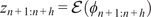 $ {z}_{n+1:n+h}=\mathrm{\mathcal{E}}\left({\phi}_{n+1:n+h}\right) $
to evaluate the transformer
$ {z}_{n+1:n+h}=\mathrm{\mathcal{E}}\left({\phi}_{n+1:n+h}\right) $
to evaluate the transformer
6: Decode to reconstruct filtered snapshots:
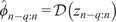 $ {\hat{\phi}}_{n-q:n}=\mathcal{D}\left({z}_{n-q:n}\right) $
7: Initialize autoregressive input for transformer:
 $ {z}_{\mathrm{input}}={z}_{n-q:n} $
8: Initialize list for predicted latent states:
 $ {\hat{z}}_{n+1:n+h}=\left[\hskip0.1em \right] $
9: for
 $ t=1 $
to
$ t=1 $
to
 $ h $
do
$ h $
do
10: Predict next latent state:
 $ {\hat{z}}_{n+t}=\mathcal{T}\left({z}_{\mathrm{input}}\right) $
11: Append prediction to list:
 $ {\hat{z}}_{n+1:n+h}.\mathrm{append}\left({\hat{z}}_{n+t}\right) $
12: Update input window for next step:
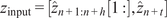 $ {z}_{\mathrm{input}}=\left[{\hat{z}}_{n+1:n+h}\left[1:\right],{\hat{z}}_{n+t}\right] $
13: end for
14: Compute total loss
 $ \mathrm{\mathcal{L}} $
15: Backpropagate gradients and update parameters of
 $ \mathrm{\mathcal{E}} $
,
$ \mathrm{\mathcal{E}} $
,
 $ \mathcal{D} $
, and
$ \mathcal{D} $
, and
 $ \mathcal{T} $
16: end for
17: end for
18: return Trained models
 $ \mathrm{\mathcal{E}} $
,
$ \mathrm{\mathcal{E}} $
,
 $ \mathcal{D} $
, and transformer
$ \mathcal{D} $
, and transformer
Model and data configuration parameters

A.3. Full-scale closure—alternative architectures
The diffusion model used as a benchmark in Section 5.2 is inspired by the original denoising diffusion probabilistic models (DDPM) framework (Ho et al., Reference Ho, Jain and Abbeel2020), where the model is trained to iteratively denoise data corrupted by Gaussian noise. The denoising network employs a U-Net style auto-encoder, using max-pooling layers and convolutional kernels of size 3 to progressively downsample input images from
 $ 64\times 64 $
and the two input channels
$ 64\times 64 $
and the two input channels
 $ \left(u,v\right) $
to a latent representation of size
$ \left(u,v\right) $
to a latent representation of size
 $ 4\times 4 $
with 256 feature channels.
$ 4\times 4 $
with 256 feature channels.
Formally, the forward noising process is defined by a noise schedule
 $ {\left\{{\beta}_t\right\}}_{t=1}^T $
, with
$ {\left\{{\beta}_t\right\}}_{t=1}^T $
, with
 $ T=1000 $
noising and denoising steps, gradually adding noise to the clean data
$ T=1000 $
noising and denoising steps, gradually adding noise to the clean data
 $ {x}_0 $
to produce noisy samples
$ {x}_0 $
to produce noisy samples
 $ {x}_t $
via
$ {x}_t $
via
 $$ q\left({x}_t|{x}_0\right)=\mathcal{N}\left({x}_t;\sqrt{{\overline{\alpha}}_t}{x}_0,\left(1-{\overline{\alpha}}_t\right)\mathbf{I}\right), $$
where
 $ {\overline{\alpha}}_t={\prod}_{s=1}^t\left(1-{\beta}_s\right) $
. The model is trained to predict the noise
$ {\overline{\alpha}}_t={\prod}_{s=1}^t\left(1-{\beta}_s\right) $
. The model is trained to predict the noise
 $ \epsilon $
added at each step by minimizing the mean squared error loss:
$ \epsilon $
added at each step by minimizing the mean squared error loss:
 $$ \mathrm{\mathcal{L}}={\unicode{x1D53C}}_{x_0,\epsilon, t}\left[\parallel \epsilon -{\epsilon}_{\theta}\left({x}_t,t\right){\parallel}^2\right], $$
where
 $ {\epsilon}_{\theta } $
is the noise predicted by the network at timestep
$ {\epsilon}_{\theta } $
is the noise predicted by the network at timestep
 $ t $
. The inference is performed by sampling from the learned reverse process starting from Gaussian noise conditioned on the filtered data, reconstructing clean samples through iterative denoising. Training utilizes the Adam optimizer over 2000 epochs. Conceptually, the diffusion model learns a parameterization of the reverse conditional Gaussian transitions that gradually remove noise. These Gaussian transitions are defined directly in the original high-dimensional input space.
$ t $
. The inference is performed by sampling from the learned reverse process starting from Gaussian noise conditioned on the filtered data, reconstructing clean samples through iterative denoising. Training utilizes the Adam optimizer over 2000 epochs. Conceptually, the diffusion model learns a parameterization of the reverse conditional Gaussian transitions that gradually remove noise. These Gaussian transitions are defined directly in the original high-dimensional input space.
The Variational Auto-Encoder (VAE) used as the other benchmark in Section 5.2 is motivated by the assumption that the data distribution lies on a low-dimensional manifold, as is often the case in dynamical systems applications. The VAE also aims to approximate the posterior distribution of the latent variables given the observed data
 $ {x}_{\mathrm{data}} $
by learning parameters
$ {x}_{\mathrm{data}} $
by learning parameters
 $ \left({\mu}_{\theta },{\Sigma}_{\theta}\right) $
of a Gaussian distribution in a latent space of significantly lower dimensionality than the original input space (Kingma and Welling, Reference Kingma and Welling2013), unlike Diffusion models. This low-dimensional representation facilitates much more efficient inference and captures the essential structure of the data. It does, however, rely on a strong hypothesis that such a low-dimensional projection exists. The VAE employed in this work is a fully connected neural network that gradually compresses the input data from dimension
$ \left({\mu}_{\theta },{\Sigma}_{\theta}\right) $
of a Gaussian distribution in a latent space of significantly lower dimensionality than the original input space (Kingma and Welling, Reference Kingma and Welling2013), unlike Diffusion models. This low-dimensional representation facilitates much more efficient inference and captures the essential structure of the data. It does, however, rely on a strong hypothesis that such a low-dimensional projection exists. The VAE employed in this work is a fully connected neural network that gradually compresses the input data from dimension
 $ 64\times 64 $
down to a 4-dimensional latent space. The model is trained by optimizing the variational lower bound, expressed as
$ 64\times 64 $
down to a 4-dimensional latent space. The model is trained by optimizing the variational lower bound, expressed as
 $$ \mathrm{\mathcal{L}}=\mathrm{KLD}\left({q}_{\theta}\left(z|X\right)\parallel p(z)\right)-{\unicode{x1D53C}}_{z\sim {q}_{\theta }}\left[\log {p}_{\theta}\left(X|z\right)\right], $$
where
 $ {q}_{\theta}\left(z|X\right) $
is the approximate posterior,
$ {q}_{\theta}\left(z|X\right) $
is the approximate posterior,
 $ p(z) $
the prior, and
$ p(z) $
the prior, and
 $ {p}_{\theta}\left(X|z\right) $
the likelihood. In practice, we introduce a weighting factor on the Kullback–Leibler divergence term to prioritize accurate reconstruction over strict adherence to Gaussianity in the latent space, thus balancing the trade-off between fidelity and regularization. The weighting factor used in this example is
$ {p}_{\theta}\left(X|z\right) $
the likelihood. In practice, we introduce a weighting factor on the Kullback–Leibler divergence term to prioritize accurate reconstruction over strict adherence to Gaussianity in the latent space, thus balancing the trade-off between fidelity and regularization. The weighting factor used in this example is
 $ 0.01 $
. The value of 0.01 was chosen empirically to balance reconstruction accuracy and latent-space regularization. A small KL weight was found to sufficiently encourage a smooth latent distribution without degrading reconstruction quality, which is critical for accurate downstream dynamics prediction and closure mapping.
$ 0.01 $
. The value of 0.01 was chosen empirically to balance reconstruction accuracy and latent-space regularization. A small KL weight was found to sufficiently encourage a smooth latent distribution without degrading reconstruction quality, which is critical for accurate downstream dynamics prediction and closure mapping.


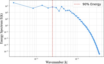

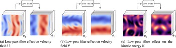
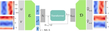
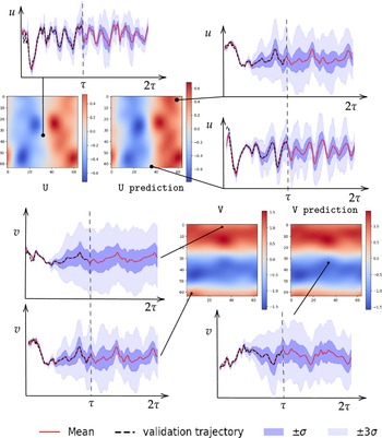


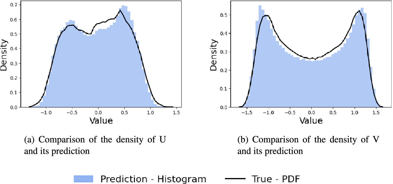


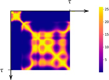

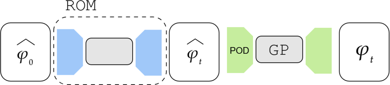


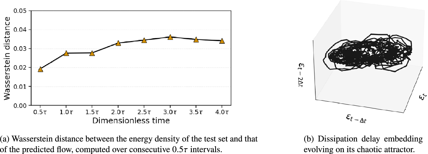
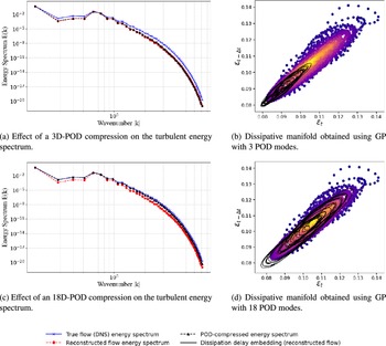
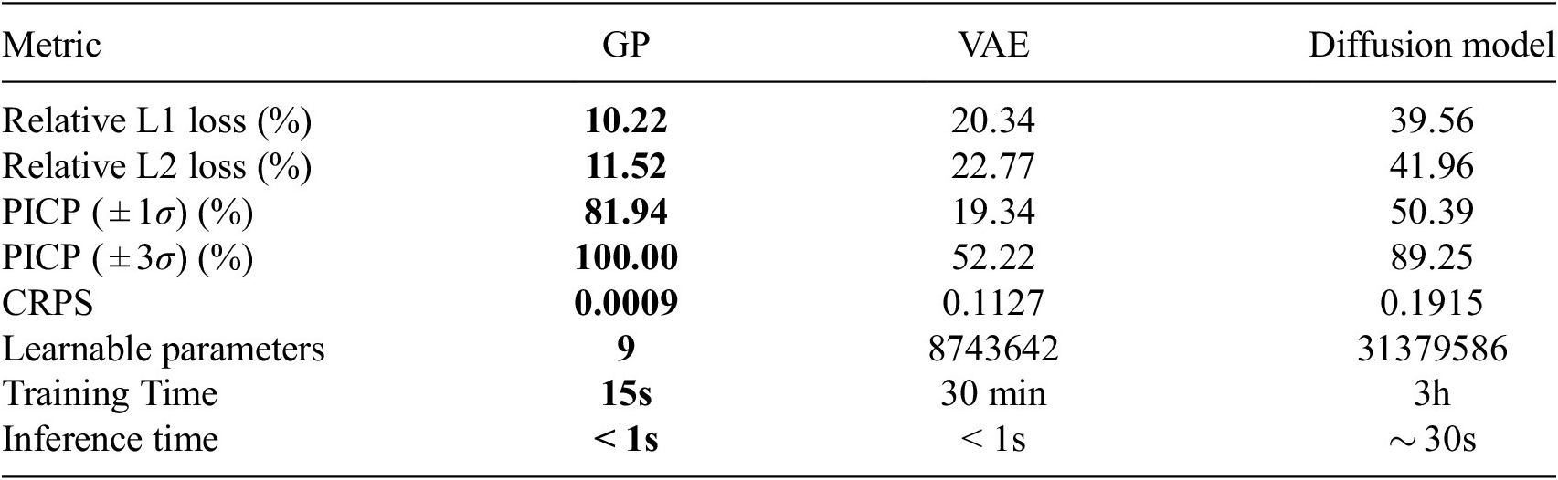
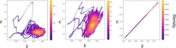


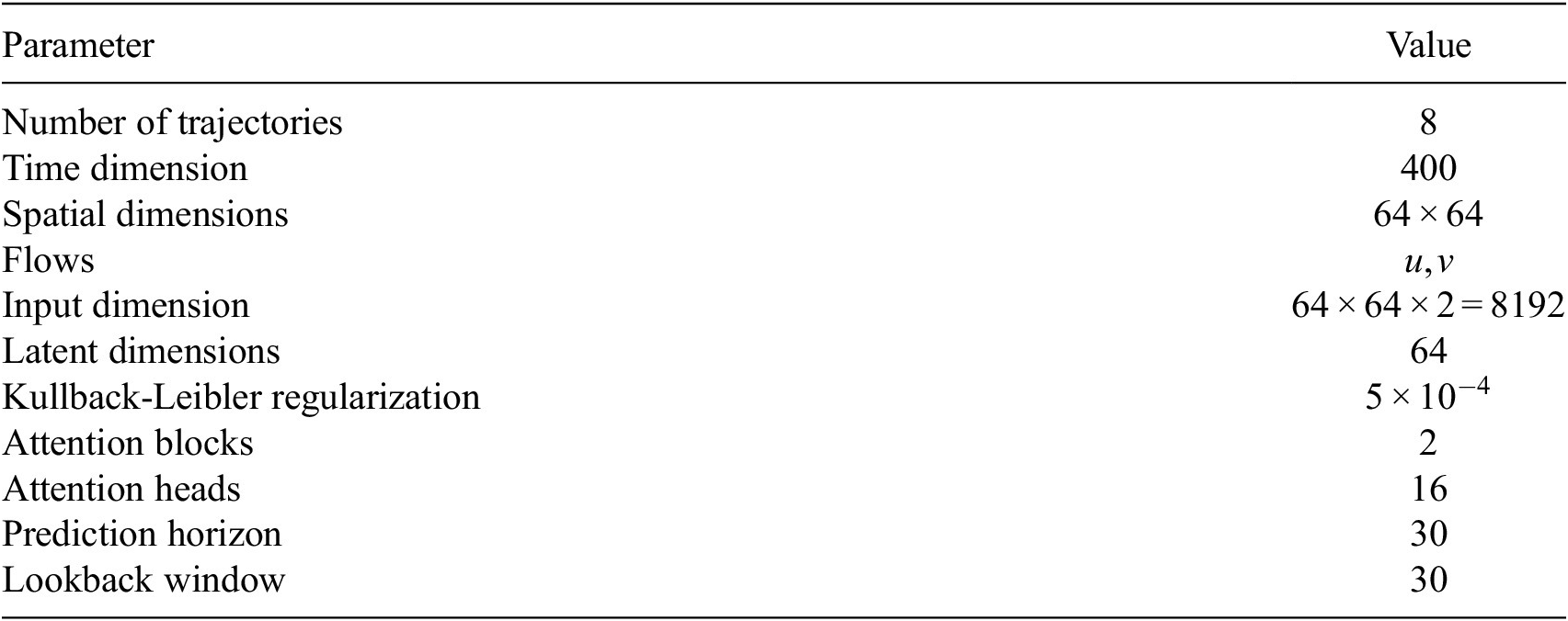

 Open access
Comments
No Comments have been published for this article.