

1. INTRODUCTION
Mars exploration missions play an important role in future deep space exploration activities, and the number of countries and international organisations, which have begun to focus planetary exploration activities on Mars is increasing. Several future international space missions have as an objective the return of Mars surface samples to the Earth (Lévesque and de Lafontaine, Reference Lévesque and de Lafontaine2007). There are many key scientific goals for Mars explorations in order to deepen the understanding of the solar system formation process and the origin of life, such as the search for water and characterisation of aqueous processes on Mars, the study of mineralogy and weathering of the Martian surface, and the search for preserved biosignatures in Martian rocks (Burkhart et al., Reference Burkhart, Ely, Duncan, Lightsey, Campbell and Mogensen2005; Li et al., Reference Li, Jiang and Liu2014). However, most of the preselected target sites for the key scientific goals are located at high elevations on the surface of Mars at close proximity to scientifically interesting terrain (Braun and Manning, Reference Braun and Manning2007). If these sites are surrounded by hazards, the lander needs to be precisely delivered from the Mars entry point (defined as a radius of 3,522 km from the centre of Mars, and an altitude of 125 km over the surface) to the preselected target site with a 100 m level through the general Mars Entry, Descent, and Landing (EDL) phase of the mission. Looking at past missions, the landing ellipse of the Viking mission was in the order of several hundred kilometres by adopting an Inertial Measurement Unit (IMU) using dead reckoning navigation mode and an unguided ballistic trajectory, which cannot meet the requirements of future manned Mars landing and sample return missions (Marschke et al., Reference Marschke, Crassidis and Lam2008; Wang, Reference Wang2011). Other past missions (Pathfinder; Mars Exploration Rover, MER; Phoenix) used non-lifting trajectories focused only on safe landing, whose landing ellipses were 200 km x 100 km, 80 km x 12 km and 100 km x 21 km, respectively (Steinfeldt et al., Reference Steinfeldt, Grant, Matz, Braun and Barton2010). The Mars Science Laboratory (MSL), whose landing ellipse is 25 km x 20 km, was launched in 2011 and landed on Mars in 2012 (Vasavada et al., Reference Vasavada, Chen, Barnes, Burkhart, Cantor, Dwyer-Cianciolo, Fergason, Hinson, Justh, Kass, Lewis, Mischna, Murphy, Rafkin, Tyler and Withers2012; Dutta and Braun, Reference Dutta and Braun2014). So advanced high-precision autonomous navigation and active aerodynamic lift control are essential and need to be well researched (Kozynchenko, Reference Kozynchenko2011; Fu et al., Reference Fu, Yang, Xiao, Wu and Zhang2015; Li and Peng, Reference Li and Peng2011; Hormigo et al., Reference Hormigo, Silva and Câmara2008).
During the EDL phase, there are three most significant sources of landing position inaccuracy on Mars (Lévesque, Reference Lévesque2006; Prince et al., Reference Prince, Desai and Queen2011): firstly, position and velocity errors at the atmospheric entry point; secondly, uncertainties in the Martian atmospheric density and the vehicle aerodynamic characteristics during the Mars entry phase and thirdly, drifts caused by strong winds during the parachute descent phase. So the Mars entry phase is the most important and dangerous period during the EDL phase. In order to address the first two significant sources of error, Mars entry navigation technologies play an important role during the whole of a precise landing mission (Li et al., Reference Li, Jiang and Liu2014; Braun and Manning, Reference Braun and Manning2007). However, there are three prerequisites affecting Mars entry navigation accuracy: firstly, an accurate Mars entry dynamic model; secondly, sufficient measurement data from the high precision sensors and thirdly, robust state estimation methods. From previous research (Fu et al., Reference Fu, Yang, Xiao, Wu and Zhang2015; Lévesque, Reference Lévesque2006), three uncertain parameters, which are Martian atmospheric density, ballistic coefficient and lift-to-drag ratio, influence the accuracy of the Mars entry dynamic model. What is more, because most sensors are blocked by the vehicle's heat shield and plasma sheath, only the IMU is available during the Mars entry phase. Fortunately, it has been found that the plasma sheath around the vehicle has little effect on Ultra-High Frequency (UHF) band (300~3,000MHZ) radio communication (Burkhart et al., Reference Burkhart, Ely, Duncan, Lightsey, Campbell and Mogensen2005). In other words, UHF radio communication can be used in the Mars entry phase to enhance the measurement data. As a result of that, a robust state estimation method is needed to effectively reduce the adverse impact of initial state errors and system model parameter uncertainties, and improve Mars entry navigation accuracy.
In the last decade, in order to overcome the adverse effects of parameter uncertainties on state estimation for Mars entry navigation, some research into state estimation methods has been conducted by researchers in different countries and international organisations. Ely et al. (Reference Ely, Bishop and Dubois-Matra2001) use a Hierarchical Mixture-of-Experts (HME) filter bank as the Mars entry navigation method, in which the filters are parameterised with various atmospheric density and other vehicle parameters. Dubois-Matra and Bishop (Reference Dubois-Matra and Bishop2004) applied a multi-model structure comprised of an Extended Kalman Filter (EKF) bank architecture to address the atmospheric density model uncertainty in the Mars entry precision navigation. A Multiple Model Adaptive Estimation (MMAE) method is adopted for Mars entry navigation in order to deal with the Martian atmospheric density high uncertainty by Zanetti and Bishop (Reference Zanetti and Bishop2007). In another study (Marschke et al., Reference Marschke, Crassidis and Lam2008), the sensor bias and scale factors are extended to the vehicle state and estimated through the MMAE method during the Mars entry phase. Recently, Li et al. (Reference Li, Jiang and Liu2014) adopted a Modified MMAE to address the atmospheric density model uncertainty using integrated navigation. From previous research mentioned above, it is found that there are four common themes. The first one is that all the research is based on the MMAE method, which uses several EKFs running in parallel. As we know, EKF has two major issues (Li and Peng, Reference Li and Peng2011; Lévesque, Reference Lévesque2006): firstly, complex Jacobin matrix calculation is needed and secondly, first-order linearization of the nonlinear system is used. However, for the Mars entry strongly nonlinear navigation system model, using first-order linearization will lead to truncation errors which cause filter divergence, and there is no guarantee that even second order terms can compensate for such errors (Khairnar et al., Reference Khairnar, Nandakumar, Merchant and Desai2007). Secondly, the works mainly address the atmospheric density model uncertainty. Nevertheless, apart from this, there are ballistic coefficient and lift-to-drag ratio uncertainties affecting the landing accuracy. Thirdly, the navigation scheme for the Mars entry phase mainly adopts IMU measurement data. Finally, the IMU and radio communication measurement model does not consider measurement systematic errors.
In this context, to solve these problems, a type of radio beacon/IMU integrated navigation method based on Multiple Model Adaptive Rank Estimation (MMARE) for the Mars entry phase is researched. In order to avoid the computation of a Jacobin matrix and truncation errors from linearization, the MMARE uses several Rank Filters (RFs) running in parallel instead of EKFs. Rank filter (RF) is a rank sampling method based on the principle of rank statistics (Fu et al., Reference Fu, Xiao and Wu2014). Considering uncertainties in the Martian atmospheric density and the vehicle aerodynamic characteristics (ballistic coefficient and lift-to-drag ratio) and measurement systematic errors during the Mars entry phase, the improved Three Degree-Of-Freedom (3-DOF) dynamic model and measurement model are obtained. Based on the improved navigation system model, these problems are addressed through the MMARE. Furthermore, through the property of normal distribution, the number of RFs has been greatly reduced. The rest of this paper is structured as follows. In Section 2, the traditional Mars entry dynamic model and the improved Mars entry dynamic model are introduced. Section 3 defines the navigation measurement model considering measurement systematic errors. The navigation method of the MMARE is designed in Section 4. In Section 5, simulations are described and results are discussed. Concluding remarks are in Section 6.
2. MARS ENTRY DYNAMIC MODEL
A simplified realistic 3-DOF dynamic model of a Mars vehicle defined with respect to the Mars-centred Mars-fixed coordinate system is adopted in this Section (Li et al., Reference Li, Jiang and Liu2014; Fu et al., Reference Fu, Yang, Xiao, Wu and Zhang2015). For the sake of simplicity, there are some common assumptions for the Mars entry dynamics used in the literature (Wang, Reference Wang2011; Fu et al., Reference Fu, Yang, Xiao, Wu and Zhang2015). Those assumptions are listed as follows: 1) Mars is a spherical shape and non-rotating; 2) the Martian atmosphere is steady and non-rotating, and its density has an exponential behaviour; 3) the Mars vehicle is a point-mass vehicle with a controllable low lift-to-drag ratio.
The simplified realistic 3-DOF dynamic model of the Mars vehicle is given by
 $$\displaylines{\dot r = v\sin \gamma \cr \dot \theta = \displaystyle{{v\cos \gamma \sin \psi} \over {r\cos \lambda}} \cr \dot \lambda = \displaystyle{v \over r}\cos \gamma \cos \psi \cr \dot v = - (D^{\ast} + g_M\sin \gamma ) \cr \dot \gamma = (\displaystyle{v \over r} - \displaystyle{{g_M} \over v})\cos \gamma + \displaystyle{1 \over v}L^{\ast}\cos \phi \cr \dot \psi = \displaystyle{v \over r}\sin \psi \cos \gamma \tan \lambda + \displaystyle{{L^{\ast}\sin \phi} \over {v\cos \gamma}}} $$
where r is the distance from the Martian centre to the centre of mass of the Mars entry vehicle, θ is the longitude, λ is the latitude, v is the velocity of the Mars entry vehicle, γ is the flight path angle (FPA), ψ is the azimuth angle and φ is the bank angle.
g M is the Martian gravitational acceleration. Typically, the gravitational acceleration model needs to be more accurate and it can be obtained through the addition of spherical harmonics. Considering the J 2 item, the accuracy of the gravitational acceleration model can reach 99·95%. However, ignoring the J 2 item, the accuracy of the gravitational acceleration calculated by Newton's inverse square force is roughly 99%. Because of the short duration of the Mars entry phase, the effect of the J 2 item is negligible and the Newton's inverse square Martian gravitational acceleration is used and given by
 $$g_M = \displaystyle{\mu \over {r^2}}$$
where μ = 4·28283 × 1013 m3/s2 is the Martian gravitational constant.
D* and L* are defined by
 $$D^{\ast} = \displaystyle{1 \over 2}\rho ^{\ast}v^{2}B^{\ast}\quad L^{\ast} = \displaystyle{1 \over 2}\rho ^{\ast}v^{2}B^{\ast}L/D^{\ast}\quad B^{\ast} = \displaystyle{{C_DS} \over {m_v}}$$
where B* is the ballistic coefficient, L/D* is the lift-to-drag ratio, $C_D$
is the aerodynamic drag coefficient, S represents the vehicle reference surface area, and m
v
is the mass of the Mars entry vehicle. The exponential Martian atmospheric density model ρ* is computed as follows
$C_D$
is the aerodynamic drag coefficient, S represents the vehicle reference surface area, and m
v
is the mass of the Mars entry vehicle. The exponential Martian atmospheric density model ρ* is computed as follows
 $$\rho ^{\ast} = \rho _0^{\ast} \exp \left[ { - \bigg(\displaystyle{{r - r_s} \over {h_s}}\bigg)} \right]$$
where $\rho _0^{\ast} = 2 \times 10^{ - 4}{\rm }\, {\rm kg/}{\rm m}^3$
is the reference density, r
s
= 3437·2 km is the reference radial radius of Mars (40 km above surface) and h
s
= 7500 m is the atmospheric scale height.
$\rho _0^{\ast} = 2 \times 10^{ - 4}{\rm }\, {\rm kg/}{\rm m}^3$
is the reference density, r
s
= 3437·2 km is the reference radial radius of Mars (40 km above surface) and h
s
= 7500 m is the atmospheric scale height.
As mentioned above, one of the three significant sources of error is the vehicle aerodynamics and the atmospheric density uncertainties. From past research, the uncertainties are listed below (Spencer and Braun, Reference Spencer and Braun1996; Braun et al., Reference Braun, Powell, Engelund, Gnoffo, Weilmuenster and Mitcheltree1995): 1) the 3 − σ uncertainty of the aerodynamic drag coefficient C
D
is $ \pm 2\% $
above Mach 10 and
$ \pm 2\% $
above Mach 10 and $ \pm 10\% $
below Mach 5, and between Mach 5 and Mach 10, a linearly interpolated value for the drag coefficient uncertainty is considered, furthermore, the distribution of C
D
uncertainty is normal; 2) the uncertainty on the atmospheric density is
$ \pm 10\% $
below Mach 5, and between Mach 5 and Mach 10, a linearly interpolated value for the drag coefficient uncertainty is considered, furthermore, the distribution of C
D
uncertainty is normal; 2) the uncertainty on the atmospheric density is $ \pm 60\% $
above 100 km, and
$ \pm 60\% $
above 100 km, and $ \pm 30\% $
below 75 km, and between 75 km and 100 km, a linearly interpolated value for density uncertainty is considered, moreover, atmospheric density uncertainty is also a normal distribution; 3) the uncertainty of the lift-to-drag ratio is
$ \pm 30\% $
below 75 km, and between 75 km and 100 km, a linearly interpolated value for density uncertainty is considered, moreover, atmospheric density uncertainty is also a normal distribution; 3) the uncertainty of the lift-to-drag ratio is $ \pm 10\% $
, and its distribution is normal. From the consideration on the safety and rigour, larger 3 − σ uncertainties are chosen, which are separately
$ \pm 10\% $
, and its distribution is normal. From the consideration on the safety and rigour, larger 3 − σ uncertainties are chosen, which are separately $ \pm 10\% $
in aerodynamic drag coefficient,
$ \pm 10\% $
in aerodynamic drag coefficient, $ \pm 60\% $
in atmospheric density and
$ \pm 60\% $
in atmospheric density and $ \pm 10\% $
in lift-to-drag ratio during the whole Mars entry phase.
$ \pm 10\% $
in lift-to-drag ratio during the whole Mars entry phase.
Under this condition, the exponential Martian atmospheric density model in Equation (4) is only an approximation of the true density model. As a result of that, in order to obtain a more accurate Martian atmospheric density model, the deviation in the Martian atmospheric density model must be taken into account. The following relationship based on the work of Lévesque (Reference Lévesque2006) and Braun et al. (Reference Braun, Powell, Engelund, Gnoffo, Weilmuenster and Mitcheltree1995) can be formulated as follows
 $$\rho _0 = \rho _0^{\ast} \left( {1 + \Delta _\rho} \right)$$
where $\rho _0 $
is the improved reference density, Δ
ρ
denotes the percentage of deviation in the improved Martian atmospheric density model and it has a normal distribution.
$\rho _0 $
is the improved reference density, Δ
ρ
denotes the percentage of deviation in the improved Martian atmospheric density model and it has a normal distribution.
So the improved Martian atmospheric density model ρ can be obtained as follows
 $$\rho = \rho _{}^{\ast} \left( {1 + \Delta _\rho} \right)$$
Then applying the same process to the density model, the improved ballistic coefficient model and lift-to-drag ratio model can be respectively formulated as follows
 $$B = B^{\ast}\left( {1 + \Delta _B} \right)$$
 $$L/D = L/D^{\ast}\left( {1 + \Delta _{L/D}} \right)$$
where B is the improved ballistic coefficient, Δ B denotes the percentage of deviation in the ballistic coefficient model with normal distribution, L/D is the improved lift-to-drag ratio, Δ L/D denotes the percentage of deviation in the lift-to-drag ratio model and its distribution is also normal.
Under these conditions, the improved drag and lift accelerations can be obtained
 $$D = \displaystyle{1 \over 2}\rho v^{2}B$$
 $$L = \displaystyle{1 \over 2}\rho v^{2}BL/D$$
Taking Equations (6)–(8) into Equations (9) and (10), the following equations can be obtained
 $$D = \left( {1 + \Delta _\rho} \right)\left( {1 + \Delta _B} \right)D^{\ast} = \left( {1 + \Delta _\rho + \Delta _B + \Delta _\rho \Delta _B} \right)D^{\ast}$$
 $$L = \left( {1 + \Delta _\rho} \right)\left( {1 + \Delta _B} \right)\left( {1 + \Delta _{L/D}} \right)L^{\ast} = ( {1 + \Delta _\rho + \Delta _B + \Delta _{L/D} + \Delta _\rho \Delta _B + \Delta _\rho \Delta _{L/D} + \Delta _B\Delta _{L/D} + \Delta _\rho \Delta _B\Delta _{L/D}} )L^{\ast}$$
Neglecting second-order small terms and higher small term, Equations (11) and (12) can be rewritten as
 $$D = \left( {1 + \Delta _\rho + \Delta _B} \right)D^{\ast}$$
 $$L = \left( {1 + \Delta _\rho + \Delta _B + \Delta _{L/D}} \right)L^{\ast}$$
Based on the property of normal distribution, Equations (13) and (14) have the following relationship
 $$D = \left( {1 + \Delta _D} \right)D^{\ast}$$
 $$L = \left( {1 + \Delta _L} \right)L^{\ast}$$
where Δ D = Δ ρ + Δ B and Δ L = Δ D + Δ L/D are both normal distributions.
Given that, the 3 − σ uncertainties of Δ
D
and Δ
L/D
are $ \pm 70\% $
and
$ \pm 70\% $
and $ \pm 10\% $
, respectively. Moreover, the number of uncertain parameters is reduced from three (Δ
ρ
, Δ
B
and Δ
L/D
) to two (Δ
D
and Δ
L/D
). As a result of that, the number of RFs used in the following part can be greatly reduced.
$ \pm 10\% $
, respectively. Moreover, the number of uncertain parameters is reduced from three (Δ
ρ
, Δ
B
and Δ
L/D
) to two (Δ
D
and Δ
L/D
). As a result of that, the number of RFs used in the following part can be greatly reduced.
Hence, the improved 3-DOF model can be written as
 $$\displaylines{\dot r = v\sin \gamma \cr \dot \theta = \displaystyle{{v\cos \gamma \sin \psi} \over {r\cos \lambda}} \cr \dot \lambda = \displaystyle{v \over r}\cos \gamma \cos \psi \cr \dot v = - (D + g_M\sin \gamma ) \cr \dot \gamma = (\displaystyle{v \over r} - \displaystyle{{g_M} \over v})\cos \gamma + \displaystyle{1 \over v}L\cos \phi \cr \dot \psi = \displaystyle{v \over r}\sin \psi \cos \gamma \tan \lambda + \displaystyle{{L\sin \phi} \over {v\cos \gamma}}} $$
So the above dynamic model is rewritten with the process noise ${\bi w}$
as follows
${\bi w}$
as follows
 $$\dot{\bi x} = f ({\bi x}) + {\bi w}$$
where
 $$f\,({\bi x}) = \left[ {\matrix{ {v\sin \gamma} \cr {\displaystyle{{v\cos \gamma \sin \psi} \over {r\cos \lambda}}} \cr {\displaystyle{v \over r}\cos \gamma \cos \psi} \cr { - (D + g_M\sin \gamma )} \cr {\bigg(\displaystyle{v \over r} - \displaystyle{{g_M} \over v}\bigg)\cos \gamma + \displaystyle{1 \over v}L\cos \phi} \cr {\displaystyle{v \over r}\sin \psi \cos \gamma \tan \lambda + \displaystyle{{L\sin \phi} \over {v\cos \gamma}}} \cr}} \right]$$ ${\bi x} = \left[ {\matrix{ r & \theta & \lambda & v & \gamma & \psi \cr}} \right]^T$
denotes the entry vehicle state variable.
${\bi x} = \left[ {\matrix{ r & \theta & \lambda & v & \gamma & \psi \cr}} \right]^T$
denotes the entry vehicle state variable.
3. NAVIGATION MEASUREMENT MODEL
In this section, a radio beacon/IMU integrated navigation scheme is adopted to increase the observation information. The new observation information is the two-way range measurement obtained by the radio communication between the vehicle and an orbiter or surface radio beacon, which is pre-set on the Mars surface or the previous Mars rover of the last mission (Williams et al., Reference Williams, Menon and Demcak2012; Lightsey et al., Reference Lightsey, Mogensen, Burkhart, Ely and Duncan2008). The measurement model is shown as follows.
3.1. Inertial measurement units
Non-gravitational acceleration is obtained from the three mutually orthogonal accelerometers of the IMU directly mounted to the vehicle. The measurement model of the acceleration can be formulated as
 $$\tilde{\bi a}^B = {\bi a}^B + {\bi b}_a + {\bi \eta} _a$$
where $\tilde{{\bi a}}^{\bi B}$
is the accelerometer measurements along the body coordinate frame,
$\tilde{{\bi a}}^{\bi B}$
is the accelerometer measurements along the body coordinate frame, ${\bi a}^B$
is the true acceleration along the body coordinate frame,
${\bi a}^B$
is the true acceleration along the body coordinate frame, ${\bi b}_a$
is the accelerometer bias,
${\bi b}_a$
is the accelerometer bias, ${\bi \eta} _a$
is the accelerometer noise approximated by additive, zero-mean, uncorrelated Gaussian random variables.
${\bi \eta} _a$
is the accelerometer noise approximated by additive, zero-mean, uncorrelated Gaussian random variables.
Because the true acceleration ${\bi a}^B$
along the body frame cannot be obtained, instead, the following relationship is used (Li et al., Reference Li, Jiang and Liu2014; Lévesque, Reference Lévesque2006)
${\bi a}^B$
along the body frame cannot be obtained, instead, the following relationship is used (Li et al., Reference Li, Jiang and Liu2014; Lévesque, Reference Lévesque2006)
 $${\bi a}^B = {\bi T}_{\!V}^B {\bi a}^V$$
where ${\bi T}_{\!V}^B $
is the coordinate transformation matrix from the velocity coordinate frame to the body coordinate frame, and its detailed form, which can be seen in references (Li et al., Reference Li, Jiang and Liu2014; Wang and Xia, Reference Wang and Xia2015), is not repeated here again.
${\bi T}_{\!V}^B $
is the coordinate transformation matrix from the velocity coordinate frame to the body coordinate frame, and its detailed form, which can be seen in references (Li et al., Reference Li, Jiang and Liu2014; Wang and Xia, Reference Wang and Xia2015), is not repeated here again. ${\bi a}^V = \left[ {\matrix{ { - D} & { - L\sin \phi} & {L\cos \phi} \cr}} \right]$
is the accelerometer measurements along the velocity coordinate frame.
${\bi a}^V = \left[ {\matrix{ { - D} & { - L\sin \phi} & {L\cos \phi} \cr}} \right]$
is the accelerometer measurements along the velocity coordinate frame.
Furthermore, the accelerometer bias of IMU is $\left[ {\matrix{ {3 \times {10}^{ - 3},} & {3 \times {10}^{ - 3},} & {3 \times {10}^{ - 3}} \cr}} \right]{\rm m/}{\rm s}^2$
(Ali et al., Reference Ali, Vanelli, Biesiadecki, Biesiadecki, Maimone, Cheng, San Martin and Alexander2005; Peng, Reference Peng2011) used in this paper.
$\left[ {\matrix{ {3 \times {10}^{ - 3},} & {3 \times {10}^{ - 3},} & {3 \times {10}^{ - 3}} \cr}} \right]{\rm m/}{\rm s}^2$
(Ali et al., Reference Ali, Vanelli, Biesiadecki, Biesiadecki, Maimone, Cheng, San Martin and Alexander2005; Peng, Reference Peng2011) used in this paper.
3.2. Range measurement
Using radio communication for the Mars entry phase has been investigated (Boehmer, Reference Boehmer1998; Lou et al, Reference Lou, Fu, Wang and Zhang2014; Way et al, Reference Way, Davis and Shidner2013). The range measurement provides the distance between the entry vehicle and an orbiter or a surface beacon. However, the output of the range measurement is the pseudorange with measurement systematic errors. The pseudorange can be reconstructed as follows
 $$\tilde R{\rm =} R + b_R{\rm +} v_R$$
 $$R = \sqrt {{({\bi r} - {\bi r}_i)}^T({\bi r} - {\bi r}_i)} $$
where $\tilde R$
is the pseudorange, R is the true range between the entry vehicle and an orbiter or a surface beacon, b
R
represents the radio range bias, and it is assumed to be 200 m (Yu et al., Reference Yu, Cui and Zhu2015) in this paper, the range noise v
R
is approximated by additive, zero-mean, uncorrelated Gaussian random variables.
r
is the position vector of the entry vehicle and
r
i
is the position vector of the ith orbiter or surface beacon.
$\tilde R$
is the pseudorange, R is the true range between the entry vehicle and an orbiter or a surface beacon, b
R
represents the radio range bias, and it is assumed to be 200 m (Yu et al., Reference Yu, Cui and Zhu2015) in this paper, the range noise v
R
is approximated by additive, zero-mean, uncorrelated Gaussian random variables.
r
is the position vector of the entry vehicle and
r
i
is the position vector of the ith orbiter or surface beacon.
Recalling the navigation measurement equations from Equations (19)–(22), the navigation measurement model is defined as
 $${\bi z} = h ({\bi x}) + {\bi v}$$
where
 $${\bi z} = \left[ {\matrix{ {{\tilde{\bi a}}^B} \cr {\tilde{\bi R}} \cr}} \right]$$
 $$\tilde{\bi a}^B = \left[ {\matrix{{\tilde a_1^B ,} & {\tilde a_2^B ,} & {\tilde a_3^B } \cr } } \right]^T,\,\,\,\,\tilde{\bi R} = \left[ {\matrix{ {{\tilde R}_1,} & {{\tilde R}_2,} & { \cdots ,} & {{\tilde R}_m} \cr } } \right]^T$$
 $$h ({\bi x}) = \left[ {\matrix{ {{\bi a}^B + {\bi b}_a} \cr {{\bi R} + {\bi b}_R} \cr}} \right]$$
where ${\bi x}$
denotes the entry vehicle state variable defined in Equation (18).
${\bi x}$
denotes the entry vehicle state variable defined in Equation (18). $\tilde{\bi a}^B$
and
$\tilde{\bi a}^B$
and $\tilde{\bi R}$
are the accelerometer and pseudorange measurements, respectively. m is the number of orbiters or surface beacons used for integrated navigation.
$\tilde{\bi R}$
are the accelerometer and pseudorange measurements, respectively. m is the number of orbiters or surface beacons used for integrated navigation. ${\bi v}$
is the measurement noise.
${\bi v}$
is the measurement noise.
4. STATISTICAL ESTIMATORS
In this Section, the MMARE using a bank of RFs is proposed for the nonlinear system model with uncertain system parameters and measurement systematic errors during the Mars entry phase. Compared with the Modified MMAE, the MMARE is applied as the autonomous navigation method in this phase.
In engineering practice, a complex engineering environment will introduce uncertain system parameters to the dynamic model and the outputs from measurement sensors have measurement systematic errors, which will degrade the filter accuracy. Hence, to improve the integrated navigation accuracy during the Mars entry phase, this paper proposes a MMARE navigation filter method.
4.1. Navigation model
Based on Equations (18) and (23) described in Sections 2 and 3, the following basic framework of navigation system model for the MMARE, which involves state estimation of a discrete-time nonlinear dynamic system, can be obtained
 $${\bi x}_{k + 1} = f ({\bi x}_k) + {\bi w}_k$$
 $${\bi z}_k = h ({\bi x}_k) + {\bi v}_k$$
where ${\bi x}_k$
is the system state vector,
${\bi x}_k$
is the system state vector, ${\bi z}_k$
is the measurement vector, f(•) and h(•) are the state transition function and measurement function, respectively,
${\bi z}_k$
is the measurement vector, f(•) and h(•) are the state transition function and measurement function, respectively, ${\bi w}_k$
is the system noise vector,
${\bi w}_k$
is the system noise vector, ${\bi v}_k$
is the measurement noise vector. They are independent Gaussian noise processes and satisfy
${\bi v}_k$
is the measurement noise vector. They are independent Gaussian noise processes and satisfy
 $$\left\{ {\matrix{ {\hskip-91pt{\rm E}[{\bi w}_k] \hfill = {\bi 0} {\rm}} \cr {{\rm Cov}[{\bi w}_k, {\bi w}_j] = {\rm E}[{\bi w}_k {\bi w}_j^T ] = {\bi Q}_k \delta _{kj}} \cr \hskip-95pt{E[{\bi v}_k] = {\bi 0}{\rm}} \cr {\hskip-11pt{\rm Cov}[{\bi v}_k,{\bi v}_j] = E[{\bi v}_k{\bi v}_j^{\rm T} ] = {\bi R}_k\delta _{kj}{\rm}} \cr {\hskip-24pt{\rm Cov}[{\bi w}_k, {\bi v}_j] = E[{\bi w}_k {\bi v}_j^{\rm T} ] = {\bi 0}{\rm}} \cr}} \right.$$
4.2. Multiple model adaptive rank estimation
In this part, the MMARE for discrete-time nonlinear stochastic time-varying system with uncertain system parameters and measurement systematic errors is given. Before that, the RF based on reference (Fu et al., Reference Fu, Xiao and Wu2014) is introduced as follows.
Step 1: Time update
 $${\bi x}_{i,k/k - 1} = f ({\bi \chi} _{i,k - 1})$$
 $$\hat{\bi x}_{k/k - 1} = \displaystyle{1 \over {4n}}\sum\limits_{i = 1}^{4n} {{\bi x}_{i,k/k - 1}} $$
 $${\bi P}_{k/k - 1} = \displaystyle{1 \over \omega} \sum\limits_{i = 1}^{4n} {\left\{ {\left( {{\bi x}_{i,k/k - 1} - \hat{\bi x}_{k/k - 1}} \right)} \right.} \left. {{\left( {{\bi x}_{i,k/k - 1} - \hat{\bi x}_{k/k - 1}} \right)}^{\rm T}} \right\} + {\bi Q}_{k - 1}$$
Step 2: Measurement update
 $${\bi z}_{i,k/k - 1} = h ({\bi \chi} _{i,k/k - 1} )$$
 $$\hat{\bi z}_{k/k - 1} = \displaystyle{1 \over {4n}}\sum\limits_{i = 1}^{4n} {{\bi z}_{i,k/k - 1}} $$
 $${\bi P}_{zz} = \displaystyle{1 \over \omega} \sum\limits_{i = 1}^{4n} {\left\{ {\left( {{\bi z}_{i,k/k - 1} - \hat{\bi z}_{k/k - 1}} \right)} \right.} \left. {{\left( {{\bi z}_{i,k/k - 1} - \hat{\bi z}_{k/k - 1}} \right)}^{\rm T}} \right\} + {\bi R}_k$$
 $${\bi P}_{xz} = \displaystyle{1 \over \omega} \sum\limits_{i = 1}^{4n} {\left\{ {\left( {{\bi \chi} _{i,k/k - 1} - \hat{\bi x}_{k/k - 1}} \right)} \right.} \left. {{\left( {{\bi z}_{i,k/k - 1} - \hat{\bi z}_{k/k - 1}} \right)}^{\rm T}} \right\}$$
 $${{K}}_k = {\bi P}_{xz}{\bi P}_{zz}^{ - 1} $$
 $$\hat{\bi x}_k = \hat{\bi x}_{k/k - 1} + {K}_k({\bi z}_k - \hat{\bi z}_{k/k - 1})$$
 $${\bi P}_k = {\bi P}_{k/k - 1} - {K}_k{\bi P}_{zz}{\bi {\rm K}}_k^{\rm T} $$
where n is the dimension of system state. The rank sampling points (Fu et al., Reference Fu, Xiao and Wu2014) are given by
 $${\bi \chi} _{i,k - 1} = \left\{ {\matrix{ {\hskip-10pt{\hat{\bi x}}_{k - 1} + u_{\,p_1}{(\sqrt {{\bi P}_{k - 1}} )}_i\quad \quad i = 1, \cdots, n\quad \quad} \cr {\hskip-10pt{\hat{\bi x}}_{k - 1} - u_{\,p_1}{(\sqrt {{\bi P}_{k - 1}} )}_{i - n}{\rm} \quad i = n + 1, \cdots, 2n} \cr {{\hat{\bi x}}_{k - 1} + u_{\,p_2}{(\sqrt {{\bi P}_{k - 1}} )}_{i - 2n}\quad i = 2n + 1, \cdots, 3n} \cr {{\hat{\bi x}}_{k - 1} - u_{\,p_2}{(\sqrt {{\bi P}_{k - 1}} )}_{i - 3n}\quad i = 3n + 1, \cdots, 4n} \cr}} \right.$$
 $${\bi \chi} _{i,k/k - 1} = \left\{ {\matrix{ {\hskip-10pt{\hat{\bi x}}_{k/k - 1} + u_{\,p_1}{(\sqrt {{\bi P}_{k/k - 1}} )}_i\quad \quad i = 1, \cdots, n\quad \quad} \cr {\hskip-10pt{\hat{\bi x}}_{k/k - 1} - u_{\,p_1}{(\sqrt {{\bi P}_{k/k - 1}} )}_{i - n}\quad {\rm} i = n + 1, \cdots, 2n} \cr {{\hat{\bi x}}_{k/k - 1} + u_{\,p_2}{(\sqrt {{\bi P}_{k/k - 1}} )}_{i - 2n}\quad i = 2n + 1, \cdots, 3n} \cr {{\hat{\bi x}}_{k/k - 1} - u_{\,p_2}{(\sqrt {{\bi P}_{k/k - 1}} )}_{i - 3n}\quad i = 3n + 1, \cdots, 4n} \cr}} \right.$$
where $u_{p_1}$
and
$u_{p_1}$
and $u_{p_2}$
are standard normal deviator, and the weight for covariance ω is equal to
$u_{p_2}$
are standard normal deviator, and the weight for covariance ω is equal to $2\left( {u_{p_1}^2 + u_{p_2}^2} \right)$
. The tuning parameters used for filter are
$2\left( {u_{p_1}^2 + u_{p_2}^2} \right)$
. The tuning parameters used for filter are $u_{p_1} = 0.4823$
and
$u_{p_1} = 0.4823$
and $u_{p_2} = 1.1281$
(Fu et al., Reference Fu, Xiao and Wu2014).
$u_{p_2} = 1.1281$
(Fu et al., Reference Fu, Xiao and Wu2014).
Given that, as shown in Figure 1, the MMARE is designed with three modules.
Overview of the multiple model adaptive rank estimation.

The specific three modules are described below:
Module 1: Parallel filter
In this module, a bank of RFs is run in parallel. Here we only give the main parts used in the next two modules, and the other detailed parts can be seen in Equations (30)–(41).
 $$\tilde{\bi z}_k^j {\bi =} {\bi z}_k - \hat{\bi z}_{k/k - 1}^j $$
 $${\bi P}_{zz}^{\,j} = \displaystyle{1 \over {\omega}} \sum\limits_{i = 1}^{4n} {\left\{ {\left( {{\bi z}_{i,k/k - 1}^{\,j} - \hat{\bi z}_{k/k - 1}^{\,j}} \right)} \right.} \left. {{\left( {{\bi z}_{i,k/k - 1}^{\,j} - \hat{\bi z}_{k/k - 1}^{\,j}} \right)}^{\rm T}} \right\} + {\bi R}_k$$
 $$\hat{\bi x}_k^{\,j} = \hat{\bi x}_{k/k - 1}^{\,j} + {K}_k^j ({\bi z}_k - \hat{\bi z}_{k/k - 1}^{\,j} )$$
 $${\bi P}_k^{\,j} = {\bi P}_{k/k - 1}^{\,j} - {K}_k^j {\bi P}_{zz}^{\,j} {K}_k^{\,j{\rm T}} $$
where $j = \matrix{ {1,} & { \cdots,} & M \cr} $
and M is the number of the RFs. The variables with the superscript j indicate that they are obtained from the jth RF in the kth step.
$j = \matrix{ {1,} & { \cdots,} & M \cr} $
and M is the number of the RFs. The variables with the superscript j indicate that they are obtained from the jth RF in the kth step.
Module 2: Weights update
 $$W_k^j = \displaystyle{{W_{k - 1}^j \Lambda _k^j} \over {\sum\limits_{\,j = 1}^M {W_{k - 1}^j \Lambda _k^j}}} $$
where
 $$\Lambda _k^j = \displaystyle{1 \over {\sqrt {\left \vert {2\pi {\bi P}_{zz}^{\,j}} \right \vert}}} \exp \left[ { - \displaystyle{1 \over 2}{\left( {\tilde{\bi z}_k^{\,j}} \right)}^{\rm T}{\left( {{\bi P}_{zz}^{\,j}} \right)}^{ - 1}\tilde{\bi z}_k^{\,j}} \right]$$
Module 3: Information fusion
 $$\hat{\bi x}_k^{} = \sum\limits_{\,j = 1}^M {W_k^j \hat{\bi x}_k^{\,j}} $$
 $${\bi P}_k^{} = \sum\limits_{\,j = 1}^M {W_k^j \left[ {{\bi P}_k^{\,j} + \left( {\hat{\bi x}_k^{} - \hat{\bi x}_k^{\,j}} \right){\left( {\hat{\bi x}_k^{} - \hat{\bi x}_k^{\,j}} \right)}^{\rm T}} \right]} $$
The initialisation of the MMARE is given as follows:
 $$\hat{\bi x}_0^{\,j} = \hat{\bi x}_0,\,\,\; \,\,{\bi P}_0^{\,j} = {\bi P}_0,\,\,\,\,\,W_0^{\,j} = \displaystyle{1 \over M}$$
5. SIMULATION AND RESULTS
To confirm the validity of the MMARE method with uncertain system parameters and measurement systematic errors during the Mars entry phase in this paper, computer simulations and analysis have been carried out by using the MATLAB/Simulink environment. The simulation sample period/step is set to 0·5 s and the planned entry span is supposed to be 400 s during the Mars entry phase. To ensure the accuracy and reliability of simulation results, the integral differential equations use a Fourth-order Runge-Kutta algorithm. Firstly, the true state variables with process noise are produced by improved Mars entry dynamic model with uncertain system parameters in an open loop without estimation in order to establish the true trajectory. Secondly, the measurement information is generated from the observation sensors. Finally, the navigation filter using radio beacons/IMU integrated navigation scheme is set up based on the MMARE or Modified MMAE iterative computation, respectively. The navigation errors equal to the state estimation subtracting the true state variables are contrastingly analysed in this section.
One key step of the MMARE is to determine the suitable number of the filters to construct the filter bank. Based on the research in reference (Li et al., Reference Li, Jiang and Liu2014), in our simulations, we assume that the MMARE with fifteen independent RFs is enough to perform the integrated navigation. Each filter in the bank is built on a special dynamic model with difference drag acceleration deviations and lift-to-drag ratio deviations shown in Tables 1 and 2. As mentioned in Section 2, because the maximum deviations of the Martian atmospheric density, ballistic coefficient and lift-to-drag ratio are respectively ±60%, ±10% and ±10% compared with real observed data, the deviations all roughly follow a normal distribution around the nominal values. Using the property of normal distribution, through simplification and consolidation, the three deviations are reduced to drag acceleration deviation and lift-to-drag ratio deviation with ±70% and ±10% maximum deviations, respectively. Therefore, the drag acceleration deviation −70%, −35%, 0, +35% and +70% and the lift-to-drag ratio deviation −10%, 0 and +10% are respectively included into the fifteen different dynamic models in our simulations. Furthermore, given the past research (Lévesque, Reference Lévesque2006; Spencer and Braun, Reference Spencer and Braun1996; Braun et al., Reference Braun, Powell, Engelund, Gnoffo, Weilmuenster and Mitcheltree1995), the true Martian atmospheric density, ballistic coefficient and lift-to-drag ratio are assumed to be respectively 30%, 5·5% and 9·5% larger than the nominal values in our simulations.
Five dynamic models with different drag acceleration deviation Δ D .
Three dynamic models with different lift-to-drag ratio deviation Δ L/D .
The initial simulation conditions of the Mars entry vehicle are summarised in Table 3. The physical parameters of the Mars entry vehicle used in this simulation are set as follows: B* = 0·016 m2/kg, L/D* = 0·156 (Lévesque and de Lafontaine, Reference Lévesque and de Lafontaine2007). Furthermore, the number of radio beacons used for the navigation filter has been analysed by Lévesque and de Lafontaine (Reference Lévesque and de Lafontaine2007) and Pastor et al. (Reference Pastor, Gay, Striepe and Bishop2000). Based on the conclusions of the past research, three radio beacons are adopted in this paper. The inertial positions of three surface beacons are listed in Table 4 (Lévesque and de Lafontaine, Reference Lévesque and de Lafontaine2007). The radio beacon/IMU integrated navigation filter parameters are shown in Table 5 (Li et al., Reference Li, Jiang and Liu2014).
Initial entry conditions (true state) and initial estimator conditions (estimated state).
Position (longitude and latitude) of the reference surface beacons.
IMU/ radio beacons integrated navigation filter parameters.
Using the measurement data from the accelerometers and radio range for the navigation filter, the state estimation errors are computed by the Modified MMAE and MMARE. Each state estimation error from radio beacon/IMU integrated navigation is shown in Figure 2. We can clearly see that the errors of all states obtained from the MMARE are almost smaller than those obtained from the Modified MMAE. As to the states of velocity, FPA and azimuth which are influenced by the uncertain system parameters, it is also found that the three state estimation errors of the MMARE are much smaller. Furthermore, each state estimation Root Mean Squared Error (RMSE) of the Modified MMAE and MMARE is calculated from 500 independent trials and plotted in Figure 3. This shows that the accuracy of the MMARE is the higher of the two filter methods. Compared with the Modified MMAE, the MMARE can much better compensate the negative influences of the uncertain system parameters and measurement systematic errors, and enhance the integrated navigation accuracy. It is further found that the convergence speed of the MMARE is faster than that of the Modified MMAE.
State estimation errors: Modified MMAE-and MMARE- based radio beacons/IMU integrated navigation.

State estimation RMSE: Modified MMAE-and MMARE- based radio beacons/IMU integrated navigation.

In addition, the mean and covariance of the estimators are calculated from the 500 independent trials and summarised in Table 6. From this Table, it is further found that the RMSE mean and covariance of the MMARE in FPA and azimuth are obviously smaller than those of the Modified MMAE, and the FPA and azimuth estimation accuracies of the MMARE are respectively increased by 64·49% and 62·41%. With respect to the altitude and velocity estimation accuracy which are important navigation indices, the altitude estimation RMSE of the MMARE reaches 61·15 m, and the estimation accuracy is increased by 47·38% compared with the Modified MMAE. Furthermore, the velocity estimation RMSE reaches 33·63 m/s, and the estimation accuracy is increased by 71·87%.
Performance comparison of the Modified MMAE and MMARE.
In order to further confirm the validity of the MMARE method, we have completed another extremely adverse environment simulation. In this environment, the true Martian atmospheric density, ballistic coefficient and lift-to-drag ratio are assumed to be respectively 55%, 9·8% and 9% larger than the nominal values, and the other conditions remain unchanged.
With these conditions, using the radio beacon/IMU integrated navigation scheme, all state estimation errors obtained from Modified MMAE and MMARE are plotted in Figure 4. Furthermore, through 500 independent trials, each state estimation RMSE of the MMARE and Modified MMAE is calculated and plotted in Figure 5. From Figures 4 and 5, we show that the state estimation accuracy of the MMARE is higher than that of the Modified MMAE. It is also found that compared with the Modified MMAE, the MMARE has a faster convergence speed. Tables 6 and 7 summarise the mean and covariance of the two estimators calculated from the 500 independent trials. From Table 7, we further show that the RMSE mean and covariance of the MMARE in FPA and azimuth affected by uncertain system parameters are obviously smaller than those of the Modified MMAE, and the FPA and azimuth estimation errors of the MMARE are respectively decreased by 57·85% and 54·25%. With respect to the important navigation index which contains altitude and velocity estimation accuracy, the altitude estimation RMSE of the MMARE reaches 70·39 m, and the estimation accuracy is increased by 50·65% compared with the Modified MMAE. Furthermore, the velocity estimation RMSE reaches 15·74 m/s, and the estimation accuracy is increased by 91·23%. The other two state estimation accuracies are also slightly improved.
State estimation errors: Modified MMAE-and MMARE- based radio beacons/IMU integrated navigation.
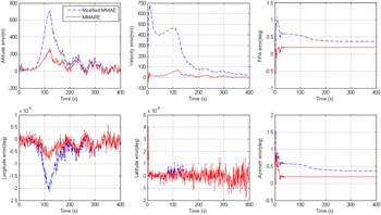
State estimation RMSE: Modified MMAE-and MMARE- based radio beacons/IMU integrated navigation.

Performance comparison of the Modified MMAE and MMARE.
Through the two simulations on different model parameter uncertainties, the MMARE can much better compensate the negative influences of the uncertain system parameters and measurement systematic errors, and enhance the navigation accuracy of the radio beacon/IMU integrated navigation, especially the altitude, velocity, FPA and azimuth estimation accuracies. In other words, the effects of the uncertain system parameters and measurement systematic errors cannot be well reduced by the Modified MMAE for the state estimation so the results obtained by the Modified MMAE are worse than those by the MMARE, even though integrated navigation is used.
6. CONCLUSIONS
In this paper, the MMARE method has been proposed to address the problems of Mars entry navigation with uncertain system parameters and measurement systematic errors. In two simulations with different model parameter uncertainties, Mars entry navigation simulations have shown that the MMARE-based navigation system mitigates the effects due to the uncertain system parameters and measurement systematic errors much better than the Modified MMAE-based navigation system. Even in the extremely adverse Mars entry environment, the estimated altitude and velocity errors reach 70·39 m and 15·74 m/s, respectively, for the MMARE-based system. The achieved performances are commensurate with the needs of future pinpoint Mars landing missions.
FINANCIAL SUPPORT
The work described in this paper was supported by National Basic Research Program of China (grant number 2012CB720000).


