


Introduction
Palaeogeographical maps (series of maps showing the landscape state for distinct time steps) are an effective way to communicate developed insights on landscape evolution (Pons et al., Reference Pons, Jelgersma, Wiggers, De Jong and De Jong1963; Zagwijn, Reference Zagwijn1986; Berendsen & Stouthamer, Reference Berendsen and Stouthamer2001; Vos, Reference Vos2015a; Pierik et al., Reference Pierik, Cohen and Stouthamer2016). Palaeogeographical maps have been compiled by various institutes and individuals, often working in parallel over the last few decades (Berendsen, Reference Berendsen2007; Van der Meulen et al., Reference Van der Meulen, Doornenbal, Gunnink, Stafleu and Schokker2013). These reconstructions show integrated knowledge from underlying observational data from many local and regional studies. Examples of such input studies are the series of soil maps, geomorphological maps and geological maps on scale 1:50,000 (e.g. Oele et al., Reference Oele, Apon, Fischer, Hoogendoorn, Mesdag, De Mulder, Overzee, Sesören and Westerhoff1983) as well as local to regional maps in professional reports, articles and academic theses (e.g. Berendsen, Reference Berendsen1982; Weerts et al., Reference Weerts, Westerhoff, Cleveringa, Bierkens, Veldkamp and Rijsdijk2005; Cohen et al., Reference Cohen, Gibbard and Weerts2014a,b; Vos, Reference Vos2015a). These datasets not only carry important information on the substrate, but also on the present and past physical landscape.
Keeping maps and datasets up to date over time is not a trivial matter. The amounts of underlying data (e.g. borehole logs, seismics, cone penetration tests (CPTs)) is ever increasing as more of it is digitised and shared in open access databases, and new data campaigns are being performed. This is especially apparent in the Dutch delta, where increasing data quantities pose challenges for synchronising and integrating information into digital public datasets and new national maps (Weerts et al., Reference Weerts, Westerhoff, Cleveringa, Bierkens, Veldkamp and Rijsdijk2005; Berendsen et al., Reference Berendsen, Cohen and Stouthamer2007; Van der Meulen et al., Reference Van der Meulen, Doornenbal, Gunnink, Stafleu and Schokker2013; Maljers et al., Reference Maljers, Stafleu, Van Der Meulen and Dambrink2015; Cohen et al., Reference Cohen, Dambrink, De Bruijn, Marges, Erkens, Pierik, Koster, Stafleu, Schokker and Hijma2017). In order to make this effective, it is important to develop and document transparent and generic workflows for combining existing map datasets and new data.
Applications that rely on soil or substrate, such as landscape archaeology, construction or groundwater quality assessment, benefit from up-to-date synthesised datasets in map format as a starting point, because these summarise vast amounts of underlying data. In addition, large amounts of older analogue source data, on which they have been based, are not always included in digital datasets. This data often has either never been digitised or is simply lost. Furthermore, since the legacy datasets were published, many areas have been levelled or overbuilt, destroying the shallow surface or making the areas difficult to access for new field campaigns.
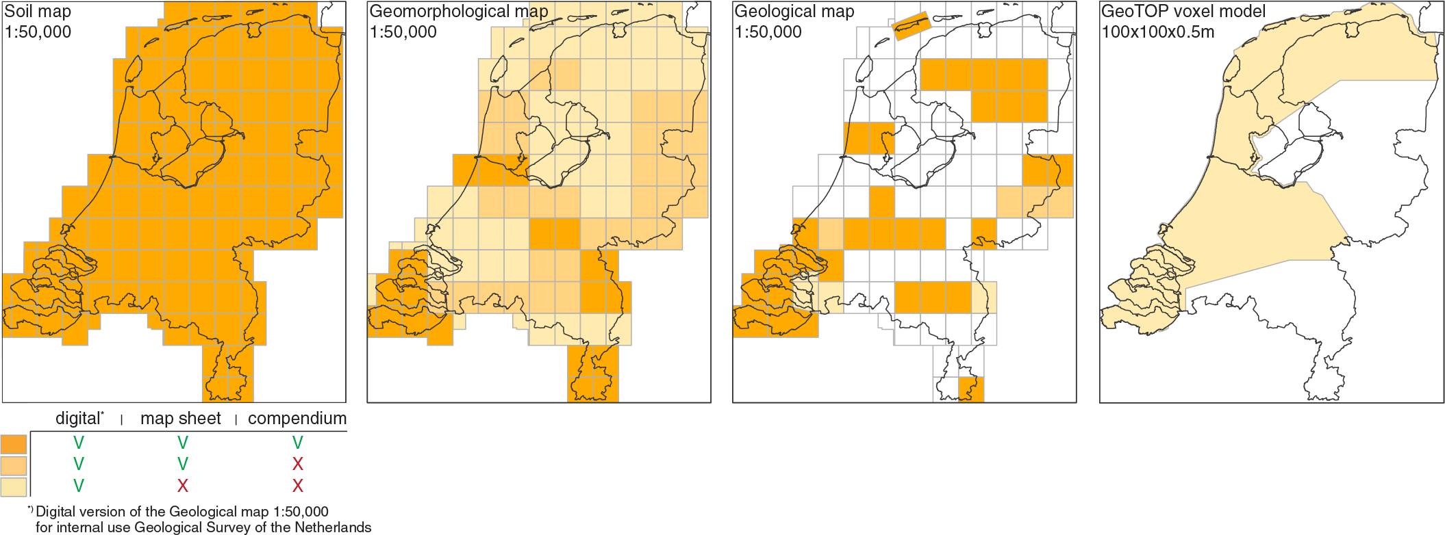
Mapping programmes over the 20th century have resulted in a large coverage of soil surveying and geological surveying map series (Figs. 1 and 2). Many map datasets have been originally created and maintained for applied and generic use, e.g. planning and design, construction, groundwater flow assessment and scientific investigation. In parallel, academic and applied research have yielded a wealth of additional geological data and insights. Over the last few decades these datasets have been digitally produced, while older originally analogue maps have been digitised. These spatial datasets and underlying data, however, vary in theme, scale, spatial coverage, observation density and resolution. It is therefore not always straightforward to combine their insights. The different themes and primary goals of the maps (e.g. pedological, geological or geomorphological; Fig. 1A), for example, mean that the same features between various maps show different boundaries or conflicting genetic interpretations. Additionally, the older maps were produced during periods when the state of knowledge was less well developed, making it in some cases hard to derive correct reinterpretations. This means that the intake and processing of such datasets into any new digital map datasets requires awareness of the scope and research strategy of the original study, against a background of general knowledge at the time.
(A) Timeline of the main mapping traditions in the Netherlands (black bars) and their products (grey produced on paper, grey-blue: digitised analogue maps; blue digitally produced). (B) Landscape subdivision with locations of selected example areas.

Spatial extent of four national mapping programmes.
Over the last few decades, data management and GIS processing have become more efficient for automatisation and uniform treatment of diverse source data (Berendsen et al., Reference Berendsen, Cohen and Stouthamer2007; Van der Meulen et al., Reference Van der Meulen, Doornenbal, Gunnink, Stafleu and Schokker2013; Pierik et al., Reference Pierik, Cohen and Stouthamer2016). As data amounts grow and workflows become more powerful and efficient, it remains important to understand the backgrounds of the combined information sources (including legacy map datasets) to assure quality control. This paper therefore reviews and compares the products of the Netherlands’ physical geographical mapping traditions (Figs 3–6), their underlying data and embedded lines of reasoning, and their original aims and purposes. We mainly focus on their use for Holocene palaeolandscape reconstructions in coastal and fluvial areas. In these most dynamic areas, incorporating legacy datasets into landscape reconstructions is relatively complicated and currently most well-developed.
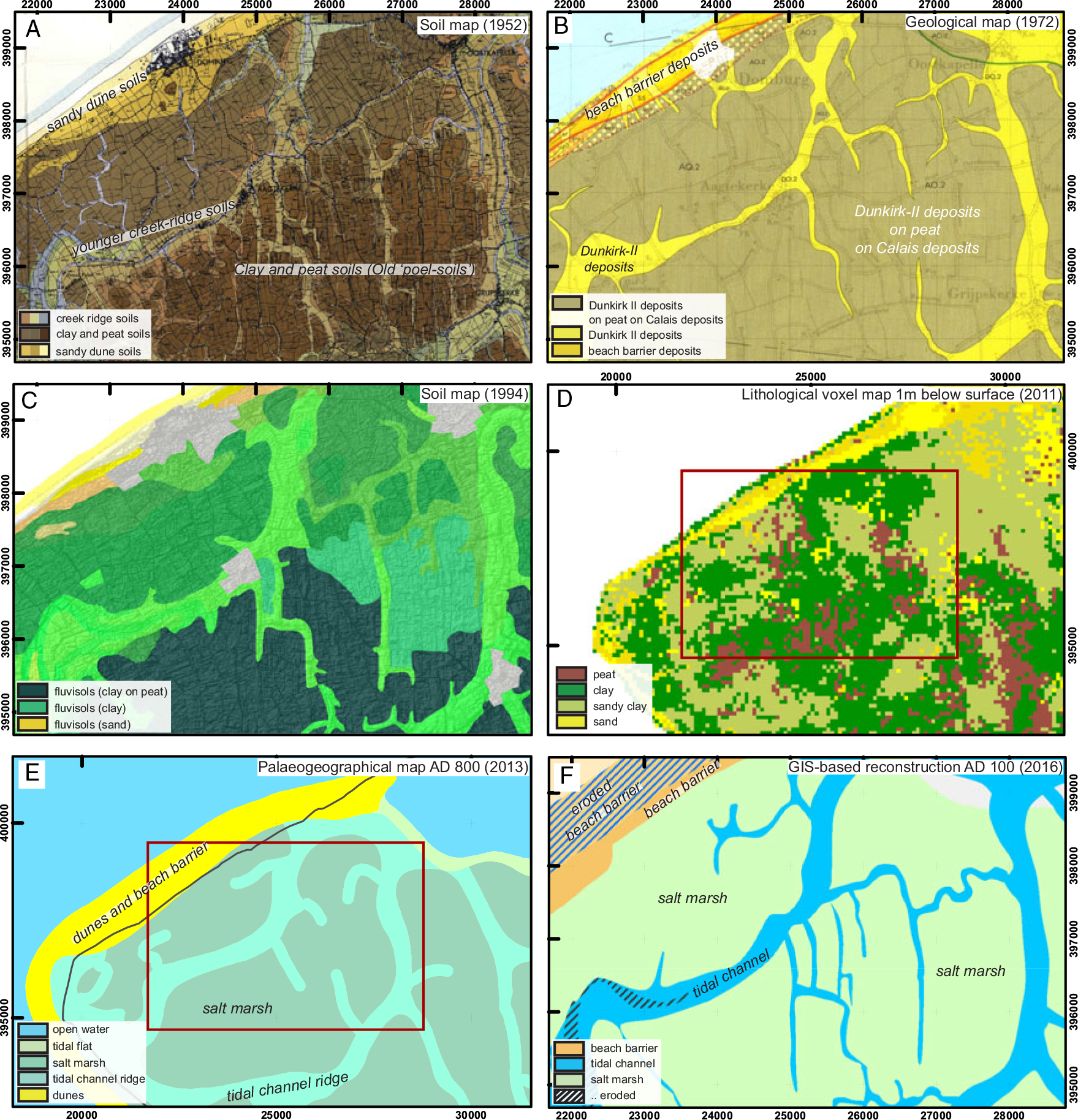
Example area of Walcheren, southwestern coastal plain (for location see Fig. 1B). Behind a narrow beach barrier in the northwest, sandy creeks dissect clayey and peaty floodbasins. Red boxes in (D) and (E) show the extent of (A–C) and (F). (A) Pedogenetic map (Bennema et al., Reference Bennema, Van der Meer, Dorsman and Van der Feen1952, original scale 1:10,000). (B) Geological map (Van Rummelen, Reference Van Rummelen1972, original scale 1:50,000). (C) Soil map (STIBOKA: Pleijter & Van Wallenburg, Reference Pleijter and Van Wallenburg1994; original scale 1:50,000). (D) GeoTOP voxel-model extracted map (Stafleu et al., Reference Stafleu, Maljers, Gunnink, Menkovic and Busschers2011; 100 × 100 m grid cells), showing the most probable lithology 0.5–1.0 m below the surface. (E) National palaeogeographical map for AD 800 (Vos & De Vries, Reference Vos and De Vries2013). (F) GIS-generated palaeogeographical map for AD 800 (Pierik et al., Reference Pierik, Cohen and Stouthamer2016). All maps have Amersfoort/RD new (EPSG:28992) projection.
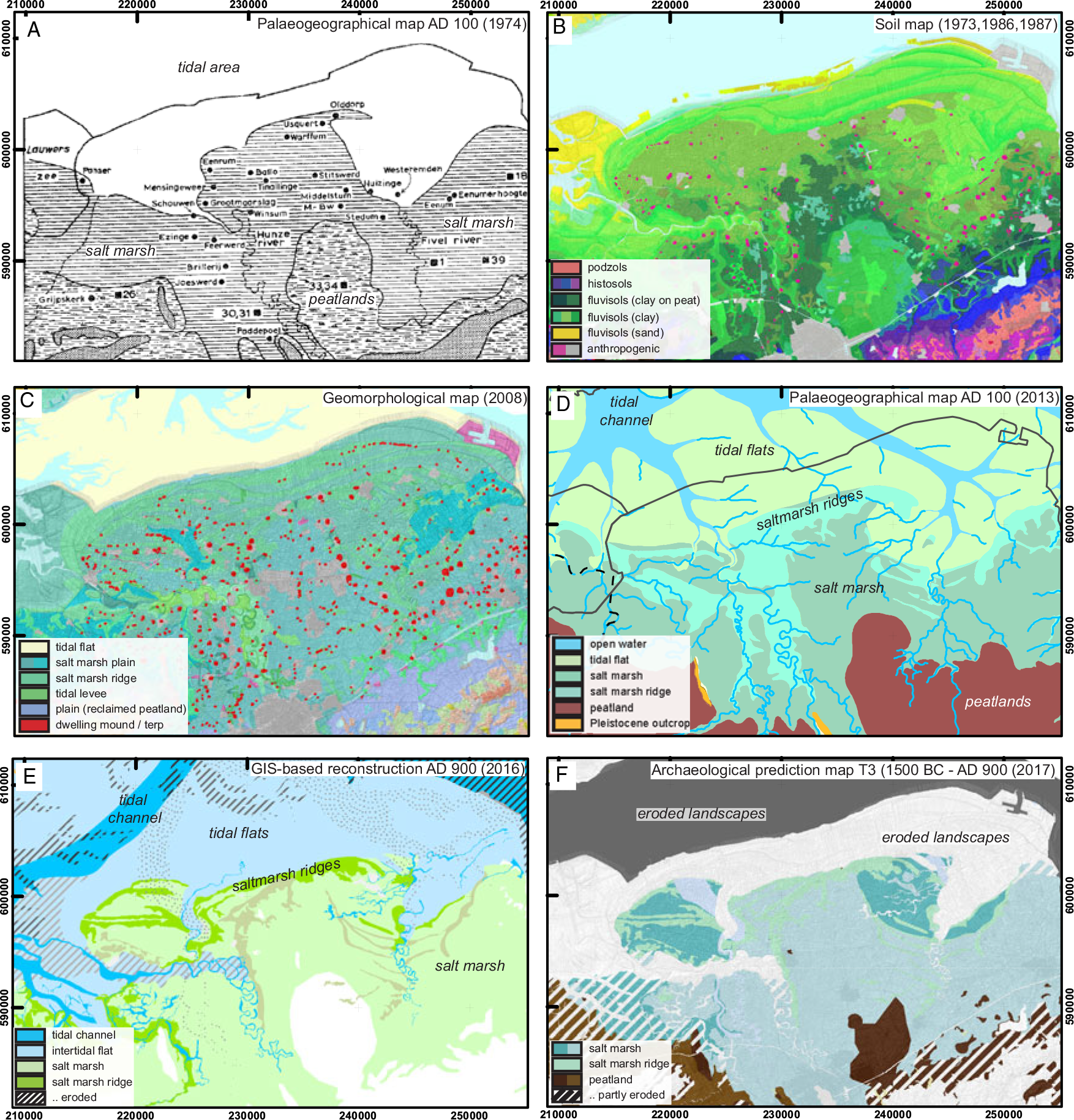
Example area in the northern coastal plain (location see Fig. 1B). In the north the Wadden Sea is situated with its tidal inlet channels and intertidal shoals. In the south, supratidal flats and flanking marsh and peatlands are present. (A) Palaeogeographical reconstruction 2000 BP of Roeleveld (Reference Roeleveld1974). (B) Soil map (STIBOKA, 1973; Clingeborg, Reference Clingeborg1986; Kuijer, Reference Kuijer1987, original scale 1:50,000), Dutch soil classification system translated to the main units of the World Reference Base for Soil Resources classification. (C) LiDAR-based geomorphological map (Koomen & Maas, Reference Koomen and Maas2004, original scale 1:50,000). (D) Palaeogeographical map for AD 100 (Vos & De Vries, Reference Vos and De Vries2013). (E) GIS-generated palaeogeographical map for AD 900 (Pierik et al., Reference Pierik, Cohen and Stouthamer2016). (F) GIS-generated landscape time-slice map (T3: 1500 BC to AD 900; Cohen et al., Reference Cohen, Dambrink, De Bruijn, Marges, Erkens, Pierik, Koster, Stafleu, Schokker and Hijma2017).
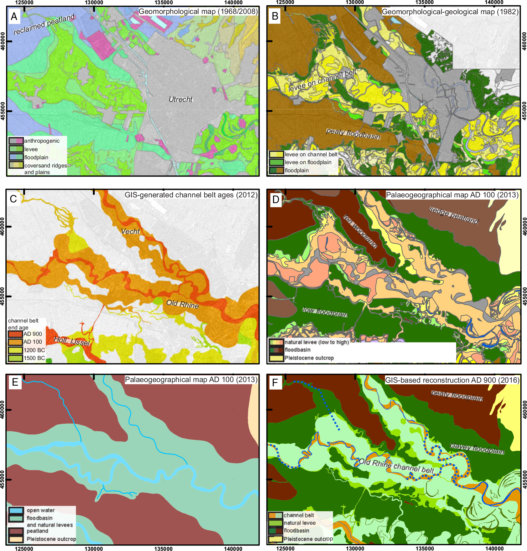
Example area in the Rhine delta around Utrecht (location see Fig. 1B). The Rhine channel belt splits in a western and northwestern branch; flow direction is towards the west (left). The channel belt is flanked by floodbasins filled with clay and peat. (A) Geomorphological map (Koomen & Maas, Reference Koomen and Maas2004, original scale 1:50,000). (B) Regional geomorphological–geological map (‘geomorphogenetical map’ (Berendsen, Reference Berendsen1982); digitised version, original scale 1:25,000). (C) GIS-generated channel-belt age map (Cohen et al., Reference Cohen, Stouthamer, Pierik and Geurts2012). (D) Regional palaeogeographical map for AD 100 (Van Dinter, Reference Van Dinter2013, original scale 1:50,000). (E) National palaeogeographical map for AD 100 (Vos & De Vries, Reference Vos and De Vries2013). (F) GIS-generated palaeogeographical map for AD 900 (Pierik et al., Reference Pierik, Stouthamer and Cohen2017a,b).
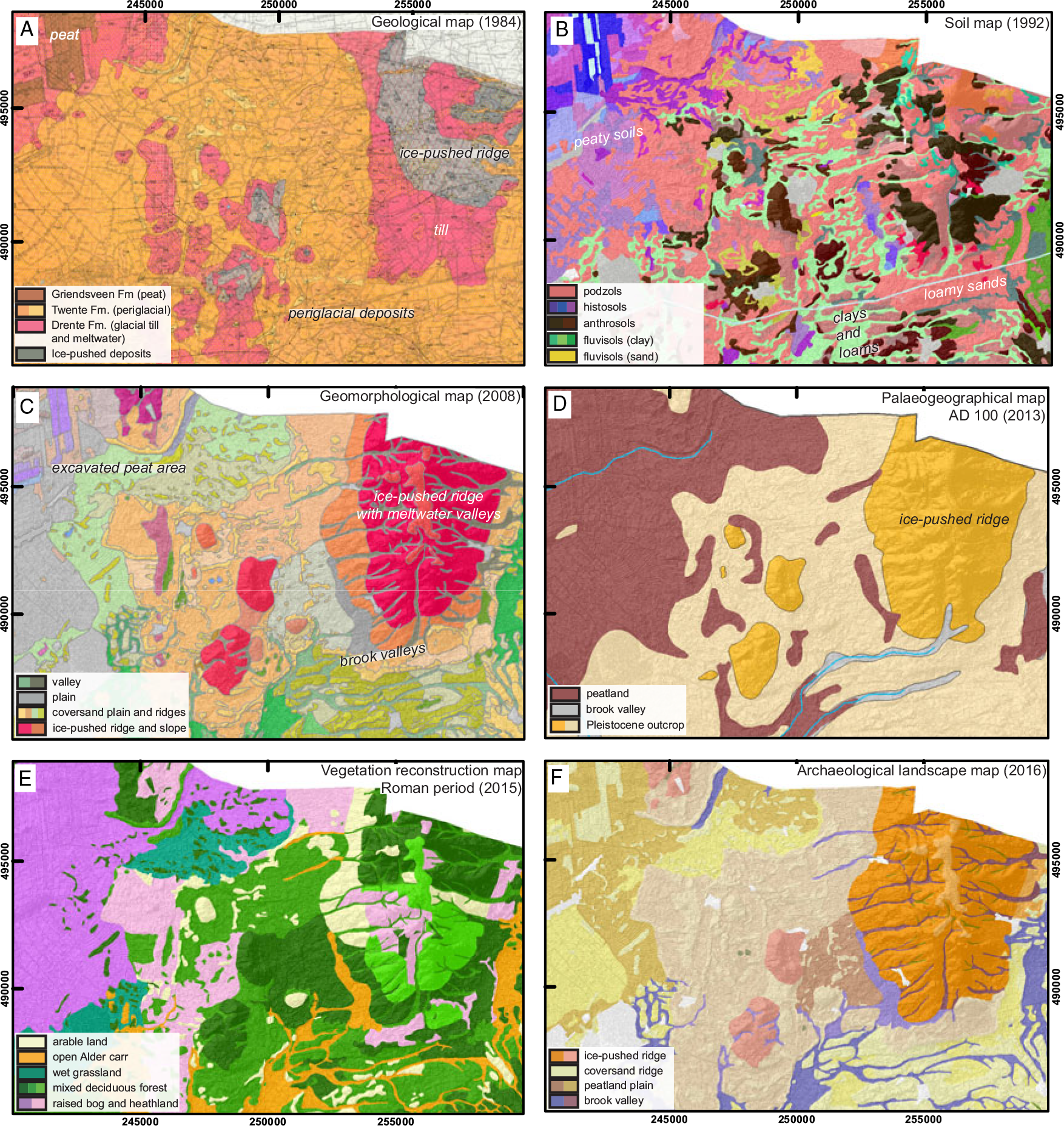
Example area of Twente (eastern Pleistocene sand area; for location see Fig. 1B), containing periglacial deposits and morphology, ice-pushed ridges, brook valleys and (mostly removed) fen peats. (A) Geological map (Van den Berg & Den Otter, Reference Van den Berg and Den Otter1993, original scale 1:50,000). (B) Soil map (STIBOKA: Ebbers & Van het Loo, Reference Ebbers and Van het Loo1992, original scale 1:50,000), Dutch soil classification system translated to the main units of the World Reference Base for Soil Resources classification. (C) LiDAR-based geomorphological map (Koomen & Maas, Reference Koomen and Maas2004, original scale 1:50,000). (D) National palaeogeographical map for AD 100 (Vos & De Vries, Reference Vos and De Vries2013). (E) Vegetation reconstruction for the Roman period (Van Beek et al., Reference Van Beek, Gouw-Bouman and Bos2015). (F) Archaeological Landscape map (Rensink et al., Reference Rensink, De Kort, Van Doesburg, Theunissen and Bouwmeester2016).
Soil, geological and geomorphological mapping traditions and their products
Before World War II, two series of national geological maps were compiled for the Netherlands (Staring, Reference Staring1858, at 1:200,000; Tesch, Reference Tesch1942, at 1:50,000). The latter was made by the Geologische Stichting, the precursor of the Geological Survey of the Netherlands. Regional map products were also created, e.g. by Harting (Reference Harting1852: subsurface of Amsterdam) and Vink (Reference Vink1926: western part of the Rhine–Meuse delta, 1:100,000). The years following World War II saw renewed efforts at systematic surveying of the Quaternary geology and soil landscape of the Netherlands. This was performed mainly for agro-economic, hydrological and civil engineering purposes, and executed by several institutions in parallel. The traditions often used combined approaches and have mutually affected each other. Their map products carry different complementary information to include in palaeolandscape reconstructions. We treat these mapping traditions in order of initiation (Fig. 1A; Table 1) and focus on detailed regional and national maps, generally with a scale of 1:50,000 or smaller. In doing so, we have split up conventional and digital geological mapping, while combining these traditions for soil maps and geomorphological maps into single sections. This is because the former two traditions have put most emphasis on age and stratigraphy, relevant for compiling palaeogeographical maps.
Relative importance of focus points within the mapping traditions; ‘+’ and ‘−’ indicate relative importance of the theme relative to the other mapping programmes. For example, in the Ages column, ‘−’ means that age information was relatively less important, while ‘+’ means it was important to assign the feature to a unit in the legend scheme.

STIBOKA = Stichting Bodemkartering (Soil Survey Institute); GSN = Geological Survey of the Netherlands; WUR = Wageningen University & Research; UU = Utrecht University.
Soil mapping
From 1933 onwards, Professor C.H. Edelman developed a survey tradition at Wageningen University that combined soil science with geological investigations, organised by the Stichting voor Bodemkartering (STIBOKA – Soil Survey Institute). After World War II, extensive mapping programmes were carried out to facilitate large-scale agricultural rationalisation and land consolidations, anticipating increases in population and food demand. The resulting pedogenetical studies aimed to characterise the soil and its parent material (upper 1 to 2 m) in high spatial detail to plan the large-scale rationalisations. In addition to soil type and lithology, these studies documented chronological information, geological–geomorphological evolution, historic land use and archaeology (Table 1). Landscape elements underlying the local soil texture differences, such as coversand ridges, residual channels, alluvial ridges and tidal levees, were mapped accurately with an average density of 8–16 observations/ha (800–1600 obs./km2) (Fig. 3A). The soil maps (scales 1:5,000; 10,000; 25,000) are available for various parts of the coastal plain (e.g. Van Liere, Reference Van Liere1948; Bennema et al., Reference Bennema, Van der Meer, Dorsman and Van der Feen1952 – Fig. 3A; Cnossen, Reference Cnossen1958; De Smet, Reference De Smet1962), the fluvial area (e.g. Edelman et al., Reference Edelman, Eringa, Hoeksema, Jantzen and Modderman1950; Pons, Reference Pons1966 – Fig. 8A, further below)) and the Pleistocene sand area (e.g. Pijls, Reference Pijls1948; Schelling, Reference Schelling1955). The mappings were upscaled to regional (province level) between the 1950s and 1970s, e.g. by Pons & Wiggers (Reference Pons and Wiggers1959/60), Van Wallenburg (Reference Van Wallenburg1966) and Pons & Van Oosten (Reference Pons and Van Oosten1974).
In 1966, STIBOKA introduced a new soil-classification system for a 1:50,000 national soil map series (De Bakker & Schelling, Reference De Bakker and Schelling1966; De Bakker, Reference De Bakker1970; Schelling, Reference Schelling1970 – Figs 3C, 4B and 6B). Similar to the earlier generation of soil maps, the system focuses on shallow-soil properties (typically to 1.2 m depth); however, it was more strictly based on describing pedological criteria. This marked a shift from geological–geomorphological based map legends to soil units based on pedological criteria (Table 1 – Hartemink & Sonneveld, Reference Hartemink and Sonneveld2013). These maps were based on dense grids of field observations (pits and corings), logged by specialists (4–8 obs./ha; 400–800 obs./km2), and, where present, data behind the earlier generation of soil maps. Borehole locations for soil profile description were chosen based upon the landscape (hydro)geomorphology, assuming that terrain and groundwater conditions affect soil formation and hence the spatial patterns of the soil map units. Following the same assumption, soil map boundaries partly follow these geomorphological units, which at the time were often more distinct than today. Compendiums made for each map sheet contain a substantial review of the shallow geology, geomorphological evolution and prehistoric and historic human land use. Throughout the 1980s, the research focus shifted more towards applied use (e.g. groundwater and soil quality), and the 1:50,000 series was made digital in 1999. It has received considerable regional updates (2000–2010s) that focused on statistical remapping. It moved away from the map sheet divisions and put more emphasis on underlying soil property data (laboratory measurements and borehole data). This shift towards a more quantitative and reproducible approach facilitated applied research themes, e.g. deterioration of peaty topsoil (Kempen et al., Reference Kempen, Brus, Heuvelink and Stoorvogel2009, Reference Kempen, Heuvelink, Brus and Stoorvogel2010).
The documentation of the soil-genetic properties and the high spatial resolution of the 1940s–60s legacy soil maps were not often equalled in more recent studies. The national coverage of the 1:50,000 national soil map series (Fig. 2) in digital form is noteworthy (De Vries et al., Reference De Vries, de Groot, Hoogerland and Denneboom2003). For example, these maps clearly show the presence of peatlands, type of peat and the clay extent on top of it, indicating past extents of tidal and fluvial floodbasins. However, the boundaries of the map units were generalised compared to the pre-1966 detailed local surveys (generally 1:5,000–1:25,000 – no national coverage). This means that where these legacy surveys had been performed, details were partially lost in the national soil map. This amount of detail of especially the older generations of soil maps could be achieved because many, nowadays partly lost, borehole data were used, supplemented with geomorphological field observations to draw accurate boundaries. Many mapped elements are not easily traceable anymore in the present-day landscape and in more recent maps, due to mechanised agricultural practices and because extensive areas have been overbuilt.
For the above reasons, the legacy soil mapping products – where available – provide relevant accurate information about the presence, age and extent of geomorphological, geological as well as archaeological elements in the landscape (e.g. De Boer et al., Reference De Boer, Molenaar and Soonius2014). For example, local pedological terms, such as ‘knikklei’ (Veenenbos, Reference Veenenbos1949) and ‘pikklei’ (De Roo, Reference De Roo1953) from the coastal plain, were also lithologically described and genetically interpreted, allowing these detailed studies to be used in modern maps. They can for example be translated into geomorphological units (e.g. soil formation in ‘heavy’ clay that formed as a supratidal flat – Vos, Reference Vos2015a; Pierik et al., Reference Pierik, Cohen and Stouthamer2016). Another example that demonstrates such interdisciplinary application can be found in the coastal plain, where information on embankment history was incorporated into the soil units. Here, topsoil and subsoil were mapped using chronostratigraphical, geomorphological and pedological criteria combined: the oldest reclaimed areas contain decalcified soils, sandy inversion ridges and clayey supratidal areas; whereas successively younger embanked tidal flats (mostly formed since the Late Middle Ages) have a higher elevation, contain more sand and have soils that have so far remained calcareous (Bennema et al., Reference Bennema, Van der Meer, Dorsman and Van der Feen1952; Pons, Reference Pons1965 – Fig. 3A). Although insights progressed over the 20th century, and assigned chronology and geological–geomorphological genesis of the mapped elements often improved in later studies (see next subsection and ‘Digital geological mapping’ and ‘Palaeogeographical research traditions and map products’ further below), the legacy soil mapping products still provide a valuable base for assessing the Dutch substrate because of their detailed nature and multidisciplinary scope.
Conventional geological mapping
The second series of geological map sheets was produced on a scale of 1:50,000, mainly serving exploration of aggregate resources (e.g. clay, sand, gravel – Faasse, Reference Faasse2002; Westerhoff, Reference Westerhoff and Floor2012). Other goals were to forecast foundation depth for construction (i.e. depth of Pleistocene sands) and to map geohydrological units (aquifers and aquitards). Geological maps of the 1:50,000 series were produced between 1964 and 2000; the programme was ended in favour of a digital mapping approach (see ‘Digital geological mapping’ below). At that time c.30% of the Netherlands had been mapped (Fig. 2). The shallow subsurface maps were mainly based on hand-drilled boreholes, but in contrast to the workflow for the soil maps, a standard grid of equally spaced boreholes was performed (on average 16 obs./km2 in the coastal and fluvial lowland area and 9 obs./km2 in the Pleistocene uplands). Map compilation was further supported by data from deeper boreholes, outcrops, CPTs, existing maps and laboratory analysis (e.g. on pollen, heavy minerals).
The new map series at scale 1:50,000 introduced the use of the so-called profile-type legend to indicate the vertical layering of the upper few metres (Hageman, Reference Hageman1963, Reference Hageman1969). The map legend was primarily inspired by a chronostratigraphical scheme (Table 1), already used at the beginning of the 20th century. This originally lithostratigraphical division had been developed for the Flemish and northernmost French coastal-plain areas by Dubois (Reference Dubois1924), Tesch (Reference Tesch1930) and Tavernier (Reference Tavernier1946, Reference Tavernier1948) (Fig. 7). It identifies an older and a younger back-barrier clastic unit (the Calais and Dunkirk Members respectively) that in most places was separated by a peat interval. This system was adopted and expanded in the Dutch national geological mapping programme. This classification system evolved with the recognition of multiple transgression subphases within the Calais Member (subunits ‘I to IV’), and multiple transgression phases in the Dunkirk Member (subunits ‘0 to III’), separated by non-deposition (i.e. soil development) and organic accumulation. All these clastic and organic layers were included in the Westland Formation (Doppert et al., Reference Doppert, Ruegg, van Staalduinen, Zagwijn, Zandstra, Zagwijn and van Staalduinen1975). With the advent of radiocarbon dating, the transgressive subphases were placed in time by dating the intercalated peat layers. The recognised transgressions were interpreted to be the result of accelerated sea-level rise events. Based on this assumption, these ages were then projected to other areas along the Dutch coast, where similar sequences of transgressive clay and regressive organics were encountered. As insights evolved over the course of the campaign, facies and environmental interpretation (e.g. Dunkirk I; supratidal deposits) were added to the legends in the newly mapped areas in the coastal plain. The presumed sea-level rise fluctuations were used to explain habitation phases in the coastal area (e.g. Louwe Kooijmans, Reference Louwe Kooijmans1974; Behre, Reference Behre2004). Because these fluctuations were presumed to be climate-driven, the transgressions in the coastal area were thought to match phases of clastic sedimentation in the Rhine–Meuse delta as well (Hageman, Reference Hageman1969). Here, the Gorkum and Tiel Members were identified to correlate with the Calais and Dunkirk Members respectively (Doppert et al., Reference Doppert, Ruegg, van Staalduinen, Zagwijn, Zandstra, Zagwijn and van Staalduinen1975). As radiocarbon-based age-control become more important for the map legend, the originally lithostratigraphic profile-type legend increasingly became chronostratigraphic (Weerts et al., Reference Weerts, Westerhoff, Cleveringa, Bierkens, Veldkamp and Rijsdijk2005 – Table 1; Fig. 7). The hybrid map legend in fact had become a genetic model, based on the underlying concept that all tidal inlets along the Dutch coast had responded more or less synchronously to a common marine forcing, i.e. variations in sea-level rise and storm intensity.
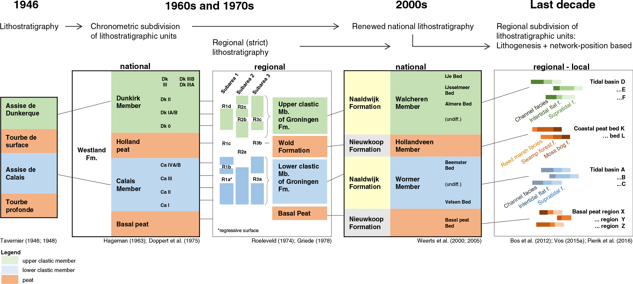
Timeline of stratigraphical division schemes in Holocene coastal geological mapping. Coastal plain stratigraphy along the Southern North Sea generally comprises basal peat, mid-Holocene clastics, intermediate peat and an upper clastic unit. This subdivision was first made for the Flemish and French coastal plain, adopted for the Netherlands and expanded with a chronometric subdivision in the 1960s and 1970s. Regionally more strict lithostratigraphical subdivision was used in the northern Netherlands, as well as in Flemish and German geological mapping. In the new millennium, chronometric subdivision was abandoned again in favour of a renewed national lithostratigraphy. As more detailed mapping occurred, mainly resulting from archaeological research, regional subdivisions of clastic members were introduced based on facies and network position (i.e. tidal system generation).
As more radiocarbon datings were performed at new sites (Groningen – Roeleveld, Reference Roeleveld1974; Rhine–Meuse delta – Berendsen, Reference Berendsen1984a,b; Zagwijn, Reference Zagwijn1986; Almere lagoon area – Van de Plassche, Reference Van de Plassche1985; Flemish coastal plain – Baeteman, Reference Baeteman1999), evidence accumulated that peat growth and clastic transgression contacts had formed much more diachronically than previously thought. Meanwhile, sedimentological studies revealed the genesis of the beach barrier coast and back-barrier (e.g. Beets et al., Reference Beets, Van der Valk and Stive1992; Van der Valk, Reference Van der Valk1992, Reference Van der Valk1996; Cleveringa, Reference Cleveringa2000). It became clear that the alternating clastics and organic beds in the coastal plain had formed as the outcome of more regional interactions between tidal and fluvial processes, storm surges and changing sediment delivery (Beets & Van der Spek, Reference Beets and Van der Spek2000). The apparent Dunkirk subphases were found to be additionally steered by human interference in coastal peatlands (Vos & Van Heeringen, Reference Vos and Van Heeringen1997; Pierik et al., Reference Pierik, Cohen, Vos, van der Spek and Stouthamer2017c). In the Rhine–Meuse delta, alternating clastics and organics could be linked to repeated avulsions creating new branches and causing abandonment of older ones. These were driven both from upstream (allocyclic) and internally (autocyclic) (e.g. Berendsen, Reference Berendsen1982; Törnqvist, Reference Törnqvist1993; Stouthamer & Berendsen, Reference Stouthamer and Berendsen2007). These new insights eventually led to a major revision of the national-scale geological mapping schemes for the Holocene deposits in the late 1990s (Weerts et al., Reference Weerts, Cleveringa, De Lang and Westerhoff2000, Reference Weerts, Westerhoff, Cleveringa, Bierkens, Veldkamp and Rijsdijk2005; De Mulder et al., Reference De Mulder, Geluk, Ritsema, Westerhoff and Wong2003 – see ‘Digital geological mapping’ below). The choice for a stricter lithostratigraphic scheme brought the national mapping systematics closer to the regional system of Roeleveld (Reference Roeleveld1974) and Griede (Reference Griede1978) (Table 1; Fig. 7) as well as those in Germany (1:25,000) and Belgium (1:50,000 – Baeteman, Reference Baeteman2005). In these countries, a stricter lithostratigraphical system was applied based on Barckhausen et al. (Reference Barckhausen, Preuss and Streif1977), with profile-type legends showing alternating clastic and organic layer sequences. These systems were neutral regarding absolute ages and superregional phase correlation. Based on the insights on avulsion, an opposite move was made for mapping the Holocene Rhine–Meuse delta. Instead of using a geological–geomorphological profile-type legend (Berendsen, Reference Berendsen1982 – next subsection), new maps became more strongly focused on age (Berendsen & Stouthamer, Reference Berendsen and Stouthamer2000, Reference Berendsen and Stouthamer2001 – ‘Digital geological mapping’ below).
Compared to soil and geomorphological national map series, the profile-type legends of the geological map sheets depict the shallow substrate to a greater depth (5 to 20 m). For the Holocene coastal plain, the geological map sheets form a consistent dataset displaying the planform geometry of Holocene generations of tidal architectural elements and their chronology (Fig. 3B). Their reuse in landscape reconstructions is particularly straightforward for the more recent map sheets on which distinct lithofacies (those of channel deposits, tidal flat deposits, etc.) were mapped separately. When using older map sheets and their compendiums, age-attributions need to be re-evaluated incorporating newer data (e.g. using 14C dates, optically stimulated luminescence (OSL) and archaeological finds – see Pierik et al., Reference Pierik, Cohen and Stouthamer2016).
Geomorphological mapping
Geomorphological maps principally show the relief (shape, elevation, slope) of the landscape and additionally contain information about landscape genesis on a general level (e.g. aeolian dune, natural levee, beach ridge) (Table 1). Between 1975 and 1993, 1:50,000 map sheets have been published in a joint effort of STIBOKA and the Geological Survey of the Netherlands (Ten Cate & Maarleveld, Reference Ten Cate and Maarleveld1977), achieving a coverage of c.60% of the country (Fig. 2). Because geomorphology reflects both soil and geological conditions, both the geological and soil mapping programmes were to benefit from this (Van den Berg, Reference Van den Berg and Floor2012). The maps were based on elevation survey maps (0.1 m intervals – Meetkundige Dienst 1942–83; scale 1:10,000), aerial photography (Von Frijtag Drabbe, Reference Von Frijtag Drabbe1954), existing soil and geological maps (see ‘Soil mapping’ above), and supplementary observations from dedicated field surveys (Koomen & Maas, Reference Koomen and Maas2004). In the early 2000s, LiDAR imagery (AHN – 1 × 1 m to 5 × 5 m footprint; cm-scale vertical resolution) was used to complete the mapping campaign on a national level (Koomen & Maas, Reference Koomen and Maas2004 – Figs 4C, 5A and 6C) and create updates (Van der Meij, Reference Van der Meij2014; Maas et al., Reference Maas, van Delft and Heidema2017). The use of LiDAR allowed the maps to become more accurate and detailed, while at the same time the digital geomorphological map product allowed larger-scale regional patterns to be queried and visualised (Koomen & Maas, Reference Koomen and Maas2004). The digital geomorphological map became widely applied in geoarchaeological studies, landscape planning (e.g. Rensink et al., Reference Rensink, De Kort, Van Doesburg, Theunissen and Bouwmeester2016 – Fig. 6F) and nature recovery projects. The LiDAR-updated areas, especially, have detailed map boundaries and genetic interpretations of surface features that are useful to conform to in palaeogeographical maps. Examples are tidal channel alluvial ridges, supratidal channels and levee relief in the coastal area (Fig. 4C), natural levees in the Rhine–Meuse delta, and coversand ridges and brook valleys in the Pleistocene uplands (e.g. Rensink et al., Reference Rensink, De Kort, Van Doesburg, Theunissen and Bouwmeester2016; Cohen et al., Reference Cohen, Dambrink, De Bruijn, Marges, Erkens, Pierik, Koster, Stafleu, Schokker and Hijma2017).
In parallel, Berendsen (Reference Berendsen1982) developed a profile-type legend for a geomorphological–geological map (‘geomorphogenetical map’) of the Holocene deltaic and flanking Pleistocene landforms in the central Netherlands (100–200 obs./km2 from borehole data by students; 1:25,000; Figs. 5B and 8B). Its hybrid system primarily used landform classifications, supplemented with lithofacies successions in the upper 2 m, using a profile-type legend (Figs. 5B and 8B) and a hatching indicating relative age of alluvial ridges. Those additions facilitated a more detailed breakdown of genetic processes and chronology of deltaic landforms, compared to the national geomorphological map series. The profile-type geomorphological maps resolved spatial continuity and position of different genetic elements of meandering river channel belts, i.e. channel bar sand, natural-levee deposits, distal floodbasin clays, and residual infill deposits of abandoned channels (Fisk, Reference Fisk1947; Allen, Reference Allen1965). They also display successions of features: e.g. floodplain deposits on levee deposits on channel belt deposits, or multiple channel belts generations within the upper 2 m below surface. The detailed information on architecture, lithofacies and chronology facilitates digital reuse for (hydro)geological applications (e.g. Bierkens & Weerts, Reference Bierkens and Weerts1994), geological–geomorphological overview maps (Berendsen & Stouthamer, Reference Berendsen and Stouthamer2001) and detailed regional palaeogeographical landscape reconstructions (Van Dinter, Reference Van Dinter2013; Pierik et al., Reference Pierik, Stouthamer and Cohen2017a,b; Fig. 5D and F – see ‘Palaeogeographical research traditions and map products’ below).
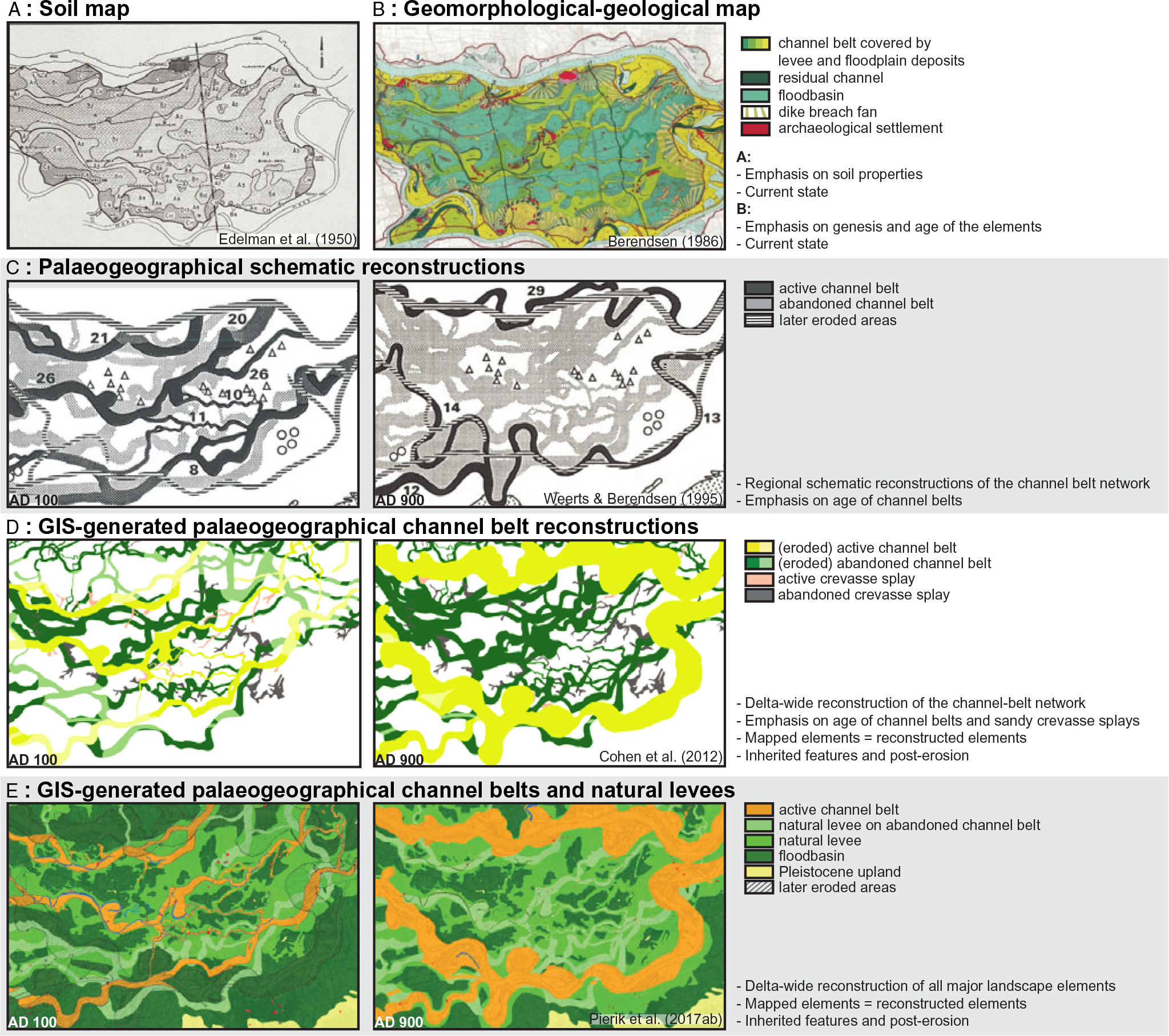
Map generations for the Bommelerwaard example area (southern part of the Rhine–Meuse delta; see Fig. 1B). (A) Soil maps of Edelman et al. (Reference Edelman, Eringa, Hoeksema, Jantzen and Modderman1950) and (B) profile-type maps of Berendsen (Reference Berendsen1986). (C) Schematic reconstruction of channel belt activity by Weerts & Berendsen (Reference Weerts and Berendsen1995). (D) GIS-generated reconstruction with focus on network history (Cohen et al., Reference Cohen, Stouthamer, Pierik and Geurts2012, update of Berendsen & Stouthamer, Reference Berendsen and Stouthamer2001). (E) GIS-generated reconstruction, added focus on natural levees (Pierik et al., Reference Pierik, Stouthamer and Cohen2017a,b).
Digital geological mapping
From the 1980s onwards, borehole data underlying shallow geological mapping had been increasingly digitised (e.g. Van der Meulen et al., Reference Van der Meulen, Doornenbal, Gunnink, Stafleu and Schokker2013). By 1997, this led to the launch of the national DINO database and web portal (Data and Information of the Netherlands’ Subsurface), at that time including 400,000 bore logs, collected by the Geological Survey. This not only made the underlying data more readily available, it also allowed systematic querying yielding new possibilities for converting geological data to construct maps for geological, hydrogeological or geotechnical purposes. The database queries aided the incorporation of field data and legacy maps into new map products, because by rearranging the data, manually tracing feature outlines became faster and more reproducible. Following more uniform and automated workflows, digital layer-stack models were created and maintained (DGM: Digital Geological Model; REGIS: hydrogeological model – Vernes et al., Reference Vernes, Van Doorn, Bierkens, Van Gessel and De Heer2005; Stafleu & Busschers, Reference Stafleu, Busschers and Floor2012; Gunnink et al., Reference Gunnink, Maljers, Van Gessel, Menkovic and Hummelman2013) and fully 3D voxel models (GeoTOP: subsurface model of the upper 30–50 m at 100 × 100 × 0.5 m resolution – Fig. 3D; Stafleu et al., Reference Stafleu, Maljers, Gunnink, Menkovic and Busschers2011, Reference Stafleu, Maljers, Busschers, Gunnink, Schokker, Dambrink, Hummelman and Schijf2012). The voxel attribute precision has been geostatistically quantified and is included in the model (Maljers et al., Reference Maljers, Stafleu, Van Der Meulen and Dambrink2015; Stafleu et al. Reference Stafleu, van der Meulen, Gunnink, Maljers, Hummelman, Busschers, Schokker, Vernes, Doornenbal, den Dulk, ten Veen, MacCormack, Berg, Kessler, Russell and Thorleifson2019). Over the last decade, the shallow subsurface 3D mapping products have become widely used by regional authorities and companies. The models have been implemented for inventories of aggregate resources (e.g. Van der Meulen et al., Reference Van der Meulen, Van Gessel and Veldkamp2005, Reference Van der Meulen, Maljers, Van Gessel and Gruijters2007; Maljers et al., Reference Maljers, Stafleu, Van Der Meulen and Dambrink2015), as schematisation input for groundwater flow modelling and salt penetration (e.g. Delsman et al., Reference Delsman, Hu-A-Ng, Vos, De Louw, Oude Essink, Stuyfzand and Bierkens2014), and as input to quantify soft subsoil geotechnical strength and susceptibility to subsidence (e.g. Koster et al., Reference Koster, Cohen, Stafleu and Stouthamer2018a,b). The geological mapping contained in these models is most highly resolved and most accurate in the upper metres, initially comparable to that in the older conventional geological map series (‘Conventional geological mapping’ above). Accuracy in revisions is improving as more field data, such as CPTs and seismic data, are included. Additional developments are integration with the DGM and REGIS models and making local models of higher resolution (e.g. 25 × 25 × 0.25 m; Stafleu et al., Reference Stafleu, van der Meulen, Gunnink, Maljers, Hummelman, Busschers, Schokker, Vernes, Doornenbal, den Dulk, ten Veen, MacCormack, Berg, Kessler, Russell and Thorleifson2019).
In the workflow to compile layer and voxel models, first, lithological intervals in boreholes were assigned a lithostratigraphical unit. Next, the upper and lower limits were interpolated between neighbouring boreholes (Stafleu et al., Reference Stafleu, Maljers, Busschers, Gunnink, Schokker, Dambrink, Hummelman and Schijf2012). For the first step, stratigraphical interpretation of existing borehole data was needed that so far had only been performed for occasional manually well-described boreholes. To automatically assign lithostratigraphy to more boreholes on a larger scale, clear new lithological and stratigraphical criteria were needed. Therefore, a new stratigraphical subdivision of the Netherlands was deemed essential (Westerhoff et al., Reference Westerhoff, Wong, Geluk, De Mulder, Geluk, Ritsema, Westerhoff and Wong2003; Stafleu et al., Reference Stafleu, Maljers, Gunnink, Menkovic and Busschers2011; Van der Meulen et al., Reference Van der Meulen, Doornenbal, Gunnink, Stafleu and Schokker2013). At the same time, this would solve the problems with the previous scheme, based on false suggestions of superregional synchronicity (‘Conventional geological mapping’ subsection above). Hence, the national stratigraphic nomenclator was considerably revised in 2000 (Weerts et al., Reference Weerts, Cleveringa, De Lang and Westerhoff2000, Reference Weerts, Westerhoff, Cleveringa, Bierkens, Veldkamp and Rijsdijk2005; Ebbing et al., Reference Ebbing, Weerts and Westerhoff2003; TNO, 2013). The new scheme was more strictly lithostratigraphic and was cleared of any intermixed chronostratigraphic conceptual knowledge. The revision was executed in line with International Stratigraphic Commission guidelines (Salvador, Reference Salvador1994). These recommend using mappable units and criteria on geographical extent and position of architectural elements, independently from any chronostratigraphical reasoning. In this way, the development to move to digital map production and geomodels after the late 1990s coincided with the trend towards a more strictly lithostratigraphic borehole data classification and map legend schemes (Table 1; see ‘Conventional geological mapping’ above).
The 2000s lithostratigraphic scheme reassigned all clastic coastal plain deposits (barrier and back-barrier deposits) to the Naaldwijk Formation (Fig. 7) and reassigned all coastal plain organic deposits to a separate formation (Nieuwkoop Fm.). Within the clastic Naaldwijk Fm., the Wormer Member and Walcheren Member were introduced as two formal Members, replacing the former Calais and Dunkirk Members respectively. This retained the originally adopted (pre-radiocarbon-dating) division into an older and a younger back-barrier clastic unit (Fig. 7), but removed all temporal subphase divisions within them. Beach-barrier and coastal dune sands (Zandvoort and Schoorl Members respectively) became part of the Naaldwijk Fm. as well. The renewed scheme also dropped the Gorkum and Tiel Members in the lower Rhine–Meuse delta, and reassigned these to the Echteld Fm. Within this formation, distinction was now made between genetic units (e.g. channel belt, overbank deposits), adopted from Berendsen (Reference Berendsen1982) and Weerts (Reference Weerts and Weerts1996 – see ’Geormorphological mapping’ above). For the central Netherlands lagoon – a major inland water body, of which great areas were reclaimed in the 20th century (former Zuiderzee) – three regionally mappable units were retained in the 2000s scheme, as Beds within the Walcheren Member. This served to continue to allow the distinction between freshwater deposits of the Almere lagoon-precursor stage (e.g. Almere Bed) and younger brackish deposits within (Zuiderzee Bed, lagoon floor clastics) and associated deposits around the lagoon (IJe Bed, storm overwash clays).
The focus on lithostratigraphy and 3D modelling meant that the current stratigraphic nomenclator for the subsurface of the Netherlands has no chronostratigraphic subsections (TNO, 2013). This means that, as with the conventional maps, additional information is still needed to correctly interpret landscape features and chronology from GeoTOP voxel models. Therefore, parallel geological mapping studies have to be consulted when age information is needed. Age information is, for example, relevant for the fields of natural and cultural heritage. This concerns national-scale map products (e.g. Deeben et al., Reference Deeben, Derickx, Groenewoudt, Peeters and Rensink2008; Vos et al., Reference Vos, Bazelmans, Weerts and van der Meulen2011), but especially products on a municipal scale, where heritage management maps have a legal status (e.g. Vos et al., Reference Vos, Rieffe and Bulten2007, Reference Vos, IJsselstijn, Jongma and De Vries2017; Lauwerier et al., Reference Lauwerier, Eerden, Groenewoudt, Lascaris, Rensink, Smit, Speleers and van Doesburg2017; Moree et al., Reference Moree, Van Trierum and Carmiggelt2018). The implementation of the Valletta Treaty on cultural heritage intensified archaeological fieldwork activities in construction projects. To reconstruct past landscapes and assess the archaeological potential of the substrate, this called for more detailed shallow geological mapping and age attribution. These studies in turn generated new data and insights, relevant for updating palaeogeographical reconstructions and geological and geomorphological research.
In the light of these developments the national lithostratigraphic scheme is used as the framework for more refined mapping on a regional and local scale (e.g. in description of exposures, palaeogeographical and geoarchaeological studies in the coastal plain (e.g. Vos et al., Reference Vos, Rieffe and Bulten2007, Reference Vos, IJsselstijn, Jongma and De Vries2017; Vos, Reference Vos2015a) and in the Rhine–Meuse delta (e.g. Gouw & Erkens, Reference Gouw and Erkens2007; Pierik et al., Reference Pierik, Stouthamer and Cohen2017a,b; Van Renswoude & Habermehl, Reference Van Renswoude and Habermehl2017)). These studies generally identify 4–10 successive clastic strata within the upper 2–3 m (Fig. 7). To identify and label the consecutive strata, they are first distinguished based on sedimentological characteristics (lithofacies) that can be coupled to a specific depositional environment (e.g. sandy deposits from intertidal flats or clayey deposits from a supratidal flat). These identified strata are then laterally traced and linked to a nearby parent tidal or fluvial channel system that delivered the sediment. In this way, it becomes possible to connect a dated salt marsh deposit to a tidal inlet with a so far unknown age, or a distal crevasse splay deposit to a meandering river branch with known ages. This spatial approach had earlier been performed on a regional scale in the Rhine–Meuse delta (Berendsen, Reference Berendsen1982) and in the coastal plain (e.g. Vos & Van Heeringen, Reference Vos and Van Heeringen1997). Applying this refinement in geological studies is increasingly becoming possible as the state of geological mapping in the Netherlands is becoming sufficiently advanced (with more open data and GIS techniques) to identify and trace deposits over large areas. This opened the way to upscale geological and palaeogeographical map products to superregional and national scales (next section – e.g. Berendsen et al., Reference Berendsen, Cohen, Stouthamer, Berendsen and Stouthamer2001, Reference Berendsen, Cohen and Stouthamer2007; Vos, Reference Vos2015a; Pierik et al., Reference Pierik, Cohen and Stouthamer2016, Reference Pierik, Stouthamer and Cohen2017a,b – Figs 3E, F and 4D). In this way, the legends of the local and regional geological maps in the coastal and delta plain have become hybrid again: ages are tied to locally to regionally recognised lithostratigraphic units, which are named and labelled in the national framework schemes. The GeoTOP voxel-models directly use the channel generations mapped in these geological age-mapping studies in the coastal and fluvial areas (‘GIS-generated palaeogeographical mapping’ below – e.g. Berendsen & Stouthamer, Reference Berendsen and Stouthamer2001; Cohen et al., Reference Cohen, Stouthamer, Pierik and Geurts2012). These serve to steer the spatial boundaries and vertical position of five different generations of fluvial and tidal channel belt systems in the substrate (Stafleu et al., Reference Stafleu, Maljers, Gunnink, Menkovic and Busschers2011; Maljers et al., Reference Maljers, Stafleu, Van Der Meulen and Dambrink2015). Vice versa, the geomodelling workflows can reveal geological elements that had not been outlined in geological maps before (e.g. Busschers et al., Reference Busschers, Stafleu, Maljers, Daniel Parsons, Ashworth, Best and Simpson2013; Schokker et al., Reference Schokker, Bakker, Dubelaar, Dambrink and Harting2015) and hence allow updating of geological age and palaeogeographical maps.
In summary, since the early 2000s we have seen stricter lithostratigraphic subdivisions of the substrate to support geomodelling workflows for novel national-scale 3D geological mapping products (Table 1). Besides lithostratigraphic identification, geological mapping on regional and local scale saw a considerable effort in administering ages and lateral tracing of the Holocene subsurface features (Fig. 7).
Palaeogeographical research traditions and map products
As more chronological data became available from the 1960s onwards, the research focus began to shift from the current state of landscape and substrate, to transient reconstructions of landscape evolution and identification of the formative processes involved (Table 1; Fig. 8). Over the last few decades, the overall accuracy and resolution of these maps have increased and they became increasingly useful for harvesting insight on rates of geomorphological processes and the extent over which they occur. The reconstructions are typically thematic, i.e. limited to selected aspects of landscape evolution (e.g. evolution of river network configuration – Berendsen & Stouthamer, Reference Berendsen and Stouthamer2001; evolution of coastal environments – Vos et al., Reference Vos, Bazelmans, Weerts and van der Meulen2011).
The task of making palaeogeographical maps requires the makers to produce a full 2D coverage of the landscape reconstructed for given moments in time, while the available or accessible data and knowledge on landscape development may neither cover the entire area nor be evenly distributed. Compiling palaeogeographical map series requires high data densities on the present state of the substrate (extent, facies interpretation and age of units), preferably evenly spread over the mapped area. To compile maps from the data, interpretations inferred from underlying direct observational data are often made (such as borehole logs, outcrop drawings, 14C dates and archaeological finds). In addition, landform inheritance and preservation have to be assessed, as well as parts of the landscape that have not survived later erosion (Berendsen et al. Reference Berendsen, Cohen, Stouthamer, Berendsen and Stouthamer2001, Reference Berendsen, Cohen and Stouthamer2007; Cohen et al., Reference Cohen, Gibbard and Weerts2014a,b, Reference Cohen, Dambrink, De Bruijn, Marges, Erkens, Pierik, Koster, Stafleu, Schokker and Hijma2017; Vos, Reference Vos2015a). This means that assumptions on the rate and spatial extent of geomorphological processes are needed to fill in those gaps. These assumptions, however, have not always been straightforward and data and insights may have been updated since the compilation effort. This means that using palaeogeographical reconstructions as input for new analyses requires evaluation of the age control and environmental interpretations of the originally available source datasets. This is especially important when these reconstructions are used to quantify rates of geomorphological processes. Such assumptions may already have been included in their compilation, feeding the risk of circular reasoning. Therefore, documentation of the input data and reconstruction workflow is crucial.
When describing the production workflow, map makers often list the materials taken into consideration, mention principles on weighing decisions and indicate spatial differences in accuracy (e.g. Vos, Reference Vos and Vos2015b). Documentation of the steps in producing palaeogeographical map series, however, is often brief and implicit. Below we describe three general types of decisions needed to make any palaeogeographical map series:
1) Each encountered preserved landform or architectural element has to be translated to a legend entry of the palaeogeographical map, e.g. a depositional environment or landscape zone at the considered time step. For example, a superficial clay bed with sandy interlayers, some marine shell storm beds and a tilled soil can represent a salt marsh landscape zone in a map for 2500 years ago or an embanked floodplain 800 years ago.
2) Blank areas within palaeogeographical maps are undesirable, and therefore non-preserved landscape elements have to be reconstructed with the best possible surrounding data and assumptions. This includes later eroded or less well-mapped areas (Vos, Reference Vos and Vos2015b). To fill such gaps, surviving broadly contemporary evidence in its surroundings is used, combined with considerations of geomorphological processes that formed these. The compiler may presume elements to have formed diachronically, and to have gradually migrated sideways.
3) The maker of the map series has to decide the time steps for which the maps will be made. A data-driven argument can be made that over the period from which features are better preserved and have allowed for more precise age control, the map series can encompass relatively short time intervals. This decision furthermore depends on the purpose of the maps. Archaeological management parties that solicit these products generally attribute greater relative importance to archaeological and historical periods in landscape evolution narratives (e.g. Bazelmans et al., Reference Bazelmans, Meier, Nieuwhof, Spek and Vos2012). From a geomorphological point of view, the desired interval spacing depends on the time span of the targeted geomorphological process. For example, tidal inlet dynamics or river avulsion may take place at different timescales (centuries to millennia) than post-glacial marine transgression (millennia), or peat bog expansion or land reclamation by humans (decades to centuries). If the time steps between consecutive reconstructions are made too large, the evolution of fast-evolving features may be missed and cannot be quantified from the map series. Incorporating more time steps would overcome this. In the case of conventional maps, the amount of required expert labour poses practical limits to this, because maps have to be redrawn manually for each time step.
Preserved landforms were generally taken or redrawn from national soil, geomorphological or geological maps. Spatial differences in the mapping accuracy of underlying datasets will affect palaeogeographical map products (e.g. deeper features from geological maps that have no national coverage). For local and regional maps, these boundaries generally have the same accuracy as these source datasets. Reconstructed (i.e. non-preserved or diachronic; decision 2) features have less accurate boundaries. For transparency these could be separately indicated on a map to show which parts of the landscape have been preserved, and which parts have not and are hence less accurate.
Data density from preserved deeper features (middle Holocene tidal or fluvial landscapes) is generally smaller than for shallow features. This, however, does not always mean that younger periods can be more accurately mapped than older periods. This is because in both the Holocene and in Pleistocene parts of the country, superficial young landscape elements have been lost through erosion, oxidation and human action. This means, for example, that diachronic peatland loss owing to Late Holocene tidal ingressions (Vos & Knol, Reference Vos and Knol2015; Vos, Reference Vos2015a; Pierik et al., Reference Pierik, Cohen and Stouthamer2016) is not substantially more or less difficult to reconstruct than middle-Holocene diachronic build-up of currently lost peatlands across the Pleistocene uplands. Also, preservation and data penetration of early and middle Holocene deposits at 4 to 15 m below the coastal plain is generally sufficient to identify main features. These generally are well-preserved (e.g. Hijma & Cohen, Reference Hijma and Cohen2011; Ten Anscher, Reference Ten Anscher2012) and allow more accurate reconstructions than inland counterpart areas with shallower and poorer preservation (e.g. Cohen et al., Reference Cohen, Dambrink, De Bruijn, Marges, Erkens, Pierik, Koster, Stafleu, Schokker and Hijma2017).
In this section, we discuss conventional manually drawn and digital GIS-generated palaeogeographical mapping techniques. Both traditions have seen more development for the coastal and fluvial area, the most dynamic and complex landscapes during the Holocene.
Conventional palaeogeographical mapping
The first manually drawn palaeogeographical maps covering the full Dutch coastal plain were compiled as a series of text figures by Pons et al. (Reference Pons, Jelgersma, Wiggers, De Jong and De Jong1963), and a second national generation was established by Zagwijn (Reference Zagwijn1986). In both publications, the selected time steps in the reconstructions coincided with the then presumed-synchronous transgression periods (see ‘Conventional geological mapping’ above). More detailed map series with regional coverage have also been made, often for geoarchaeological research and typically with a primarily geomorphological legend. Examples are Knol (Reference Knol1993 – northern Netherlands), Lenselink & Koopstra (Reference Lenselink, Koopstra, Rappol and Soonius1994 – central and northwestern coastal plain), Willems (Reference Willems1986 – upper Rhine delta) and Van Dinter (Reference Van Dinter2013 – lower Rhine delta, Fig. 5D). Thematic palaeogeographical reconstructions – channel belt network maps – were made to study maps of channel belt evolution in subregions of the Rhine delta, e.g. text figures in Berendsen (Reference Berendsen1982: SW Utrecht) and Weerts & Berendsen (Reference Weerts and Berendsen1995: Bommelerwaard – Fig. 8C). In the late 1990s, progress in digital mapping techniques and combined geomorphological and archaeological interest in resolving channel belt ages resulted in first the GIS-generated map series of the Rhine–Meuse delta channel belt network (see ‘Digital geological mapping’ above; Berendsen & Stouthamer, Reference Berendsen and Stouthamer2001; Cohen et al., Reference Cohen, Stouthamer, Pierik and Geurts2012 – Figs 5C and 8D). More regional palaeogeographical map series were compiled resulting from accumulated field surveys and (Malta-driven) archaeological studies. Examples across the coastal and fluvial area are Vos & Van Heeringen (Reference Vos and Van Heeringen1997 – Zeeland), Cohen et al. (Reference Cohen, Stouthamer, Hoek, Berendsen and Kempen2009 – Gelderse IJssel), Ten Anscher (Reference Ten Anscher2012 – Noordoostpolder), Vos & Knol (Reference Vos and Knol2015 – northern Netherlands and German Wadden coast) and Van Zijverden (Reference Van Zijverden2017 – West Frisia). In turn, these regional maps were used to update superregional- and national-scale palaeogeographical maps between 2006 and 2011 (Vos, 2006; Reference Vos2015a; Vos et al., Reference Vos, Bazelmans, Weerts and van der Meulen2011; Vos & De Vries, Reference Vos and De Vries2013 – Figs 3E, 4D, 5E, 6D). For Germany, Vos & Knol (Reference Vos and Knol2015) expanded their reconstructions along the Lower Saxonian coast, partly based on coastline reconstructions by Behre (Reference Behre2004). For the Flemish coastal plain, regional coastal reconstructions also exist (Baeteman, Reference Baeteman1999 – IJzer valley; Mathys, Reference Mathys2009 – offshore; Missiaen et al., Reference Missiaen, Jongepier, Heirman, Soens, Gelorini, Verniers, Verhegge and Crombé2016 – Scheldt Valley).
To upscale local and regional studies into a map series with national coverage, Vos et al. (Reference Vos, Bazelmans, Weerts and van der Meulen2011) prioritised high-quality geological and archaeological information obtained from a selection of the most intensely studied sites (coastal-plain ‘key sites’, cf. Vos, Reference Vos and Vos2015b). The national lithostratigraphy was often refined locally here as a framework to place dating information (see also ‘Digital geological mapping’ above). The landscape between these key sites was reconstructed using surface topographic datasets (LiDAR data; historic topographic maps) and often relies on earlier generations of geological and geomorphological mapping (Fig. 7). For the coastal plain with its complex history of shifting tidal inlets, this workflow significantly upgraded the resolution of the palaeogeographical maps compared to precursor series of the 1960s–80s. In the Rhine–Meuse delta, existing geomorphological and palaeogeographical map outlines (including Berendsen & Stouthamer, Reference Berendsen and Stouthamer2001 – see next subsection) were retraced in the national palaeogeographical maps. Across the Pleistocene uplands, phases of expanding and deteriorating inland peat cover were included (Leenders, Reference Leenders1996; Spek, Reference Spek2004; Van Beek, Reference Van Beek2009). The boundaries from the geological and geomorphological national- and regional-scale maps were often generalised for the national-scale maps (scales 1:1,000,000 to 1:500,000), yielding a lower positioning accuracy relative to that of the diverse source data considered (e.g. Figs 3E, 5E and 6D). The conventional palaeogeographical maps are manually produced visualisations of past landscapes, created for predetermined time steps. Time series of palaeogeographical maps are generally visualised for specific periods (Roman period, Early Middle Ages, etc.) and encompass typically shorter time intervals for the youngest millennia.
GIS-generated palaeogeographical mapping
Digital GIS methodologies introduced since the 1980s greatly improved the capacity to manage overloads of data because they allow faster map drawing, correction and visualisation. They facilitate (i) collecting and managing large amounts of data in digital databases; (ii) performing bulk calculations on the collected data; and (iii) generating reproducible maps automatically using scripting and map-algebra.
Analogue geological, geomorphological and soil maps have been digitised for the first decades of GIS use (Fig. 1), opening up the possibility to apply spatial analysis of the conventionally mapped units (e.g. soil and hydrological properties). Regarding automatisation techniques behind mapping workflows, 3D geomodelling at the Geological Survey (Van der Meulen et al., Reference Van der Meulen, Doornenbal, Gunnink, Stafleu and Schokker2013) was an important development (see ‘Digital geological mapping’ above). The GeoTOP voxel model, for example, is produced in a long chain of multiple scripts that use borehole databases and maps as inputs, besides applying some manual steps on input data preparation and result inspection (Stafleu et al., Reference Stafleu, Maljers, Gunnink, Menkovic and Busschers2011). Also in palaeogeographical reconstructions of the Rhine–Meuse delta, GIS techniques for feature editing, database management and workflow automatisation were used relatively early (Berendsen et al., Reference Berendsen, Cohen, Stouthamer, Berendsen and Stouthamer2001; Reference Berendsen, Cohen and Stouthamer2007) (dataset release v1: Berendsen & Stouthamer, Reference Berendsen and Stouthamer2001; v2: Cohen et al., Reference Cohen, Stouthamer, Pierik and Geurts2012). This scripted workflow generated age-based geological–geomorphological maps (Fig. 5C) and map time series of channel belt network evolution (i.e. palaeogeography) as output (Fig. 8D). Over the period 2011–16, its coverage was expanded to pre-deltaic valley landforms (Cohen et al., Reference Cohen, Stouthamer, Pierik and Geurts2012; Woolderink et al., Reference Woolderink, Kasse, Cohen, Hoek and Van Balen2018) and the Netherlands coastal plain outside the Rhine–Meuse delta (Pierik et al., Reference Pierik, Cohen and Stouthamer2016). Other datasets following the scripted age-query procedures are the geoarchaeological predictive maps for the embanked floodplains (Cohen et al., Reference Cohen, Arnoldussen, Erkens, Popta and Taal2014b) and the buried Holocene landscape dataset (Cohen et al., Reference Cohen, Dambrink, De Bruijn, Marges, Erkens, Pierik, Koster, Stafleu, Schokker and Hijma2017 – Fig. 4F). All these workflows broke with the earlier profile-type based Holocene mapping traditions and legend designs, but still used them as input (‘Conventional geological mapping’ and -‘Geormorphological mapping’ above).
The GIS-generated palaeogeographical mapping workflow essentially treats palaeogeographical output maps as a recombination of selections of geological–geomorphological elements containing numeric age information (Berendsen et al., Reference Berendsen, Cohen, Stouthamer, Berendsen and Stouthamer2001, Reference Berendsen, Cohen and Stouthamer2007; Cohen et al., Reference Cohen, Stouthamer, Pierik and Geurts2012, Reference Cohen, Arnoldussen, Erkens, Popta and Taal2014b, 2017; Pierik et al., Reference Pierik, Cohen and Stouthamer2016). Considering data management, it was therefore aimed to (i) manually maintain as few map layers as possible, and (ii) split and recombine input map layers using scripts to generate the desired map output for any list of time steps (Berendsen et al., Reference Berendsen, Cohen and Stouthamer2007; Pierik et al., Reference Pierik, Cohen and Stouthamer2016). This information is stored in one or more manually maintained digital layers (‘base maps’). For the coastal area datasets, feature outlines are imported into the base maps from established geological, geomorphological and soil maps. Apparent differences between competing source data are compared and optimised using LiDAR and borehole descriptions. For the fluvial area, borehole and LiDAR data (Berendsen & Volleberg, Reference Berendsen and Volleberg2007) are used to trace feature outlines. Ages are encoded as begin and end ages in a linked catalogue database, from which time series maps can be automatically generated. This set-up makes it possible to quickly analyse, edit and update the base maps and their encoding. Direct cross-checks are possible between the processed dating evidence (landform age assignment) and the independent interpretation from traditional geological, geomorphological and soil mapping products. This process is looped over several times to iterate the mapped and dated elements into a self-consistent map, e.g. to use all mapped and dated channel-belt fragments to generate a continuous river network for all time steps.
These datasets document and summarise large amounts of information on the position and age of Holocene rivers and tidal channels and have been used in applied and fundamental scientific research. Examples of scientific application are analysis of channel belt network dynamics (e.g. avulsion (Stouthamer & Berendsen, Reference Stouthamer and Berendsen2007; Kleinhans et al., Reference Kleinhans, Weerts and Cohen2010); tidal-ingression dynamics (Pierik et al., Reference Pierik, Cohen, Vos, van der Spek and Stouthamer2017c); post-glacial transgression and relative sea-level reconstruction (Hijma & Cohen, Reference Hijma and Cohen2011, Reference Hijma and Cohen2019; Vis et al., Reference Vis, Cohen, Westerhoff, Veen, Hijma, Van der Spek, Vos, Shennan, Long and Horton2015); sediment budgeting (Erkens & Cohen, Reference Erkens and Cohen2009; Hobo, Reference Hobo2015); and flooding dynamics (Toonen, Reference Toonen2013)).
Both conventionally produced and GIS-generated palaeogeographical maps rely on correct intake of existing soil, and both geomorphological and geological maps require additional decisions regarding the absolute and relative age of the mapped units. In GIS-derived palaeogeographical maps, these decisions are partly documented as rules stored in the scripts, as element labels in the base maps or in linked database catalogues that describe ages, source datasets and element-specific decisions. Because begin and end ages of feature activity are stored, map series of landscape elements that were actively formed can be generated for any time slice of choice (decision 3; see introduction to this section). This makes it possible to visualise which features were actively forming at a given moment and which older features by that time were fossilised or affected by younger erosional channels (automising decision 2 – Cohen et al., Reference Cohen, Arnoldussen, Erkens, Popta and Taal2014b; Pierik et al., Reference Pierik, Cohen and Stouthamer2016). This not only makes reconstruction more generic, it also avoids the effort of manual redrawing of the same feature for multiple time steps in the map series. The general and site-specific rules behind the workflow are well-documented; these rules comprise how the present state of the substrate combined with process knowledge leads to decisions in map making (Berendsen et al., Reference Berendsen, Cohen and Stouthamer2007; Pierik et al., Reference Pierik, Cohen and Stouthamer2016; Cohen et al., Reference Cohen, Dambrink, De Bruijn, Marges, Erkens, Pierik, Koster, Stafleu, Schokker and Hijma2017). By creating such map series, direct cross-checks are made between the processed dating evidence (landform age assignment) and the independent lithostratigraphical and morphogenetic interpretation from traditional geological and geomorphological mapping (decision 1; see introduction to this section). Lastly, because features are digitally copied rather than manually retraced, the spatial accuracy of the generated palaeogeographical map series is the same as that of the geological–geomorphological mappings in the source base maps, as are mapping-quality differences within the source map. Aesthetically this may be displeasing compared to conventionally produced more cartographically uniform maps, but for scientific use this is an advantage since well-mapped subareas keep their original resolution and their quality is not demoted because other areas have less data or lower-resolution input datasets.
Both the digital palaeogeographical mapping tradition and lithostratigraphy querying in 3D geomodelling use scripts to query base maps and databases. They also incorporate outlines of geological features from legacy conventional geological maps. They furthermore exchange outlines and generation of features: facies interpretation and spatial correlation from lithostratigraphical mapping is used as the starting point for base maps in palaeogeographical applications (Berendsen et al., Reference Berendsen, Cohen, Stouthamer, Berendsen and Stouthamer2001; Pierik et al., Reference Pierik, Cohen and Stouthamer2016). In turn, the base map products of the digital palaeogeographical tradition are used as input into the national-scale 3D geomodelling (e.g. ‘channel belt generations’ in Echteld and Naaldwijk Formations; see ‘Digital geological mapping’ above). An example of digital geological map products that benefited from iterative geomodelling and palaeogeographical mapping is provided by the archaeological landscape maps of Cohen et al. (Reference Cohen, Dambrink, De Bruijn, Marges, Erkens, Pierik, Koster, Stafleu, Schokker and Hijma2017; Fig. 4F), in which 3D geomodelling output and palaeogeographical datasets were used in combination on a national scale. A major thematic difference between the two traditions is the importance of lithological variation in geomodelling (stochastic output for voxel cells, quantified compositional heterogeneity; e.g. Maljers et al., Reference Maljers, Stafleu, Van Der Meulen and Dambrink2015) versus the importance given to ages and stages of development in digital palaeogeographical reconstruction (initial and matured size, duration of abandonment stage, continued visibility as a residual landform, complete burial; e.g. Cohen et al., Reference Cohen, Arnoldussen, Erkens, Popta and Taal2014b; Pierik et al., Reference Pierik, Cohen and Stouthamer2016).
Discussion
Over the 20th century, mapping traditions have evolved in different themes and between different institutes. Regardless of their originally intended use, nearly all datasets described here have seen usage for multiple purposes, both in academic and applied contexts. Some of these traditions and applications rank lithology and lithogenesis as the principal properties to map and model, while others consider age information to be equally important. Still, the soil, geomorphological, geological and palaeogeographical mapping traditions each resulted in map products conveying generic landscape information that are complementary to each other. Newer traditions seldom performed completely new data collection campaigns and often adapted and updated previously revealed patterns in the shallow surface instead from earlier mapping products. For example, data from soil mapping has been considered in shallow geological feature mappings, and information from palaeogeographical mapping has been used to import channel belt architectural elements in 3D models.
The historic development of the research traditions was driven by data availability and methodological innovations, but also by shifted user demand. Here we first summarise the main demand- and data-driven developments behind the traditions and then suggest future steps to keep on getting the best out of all accumulated data.
Societal-demand driven developments
Shifting needs from society have stimulated institutes to update map production workflows, to incorporate insights generated in parallel traditions and to move towards open data-publishing policies.
After World War II, the soil, geomorphological and geological mapping traditions were revolutionised as food production gained attention and economic activities (agriculture, mining) strongly increased. Soil survey studies were used to assess the fertility of the soil, suitability for crops, and groundwater conditions. At that time, agriculture was a relatively larger part of the Dutch economy. Also, the agricultural landscape was restructured to make yields more efficient to feed the rising population and eliminate the risk of crop failure and famine. The wealth of additional information on shallow geology and landscape evolution from these soil mapping campaigns was subsequently partially used in 1:50,000 geomorphological and geological map sheets, made for planning, construction works and mining. The responsible institutes and universities covering these themes saw a large increase in capacity facilitating thorough and systematic field campaigns that laid the foundation for all modern map products (Faasse, Reference Faasse2002; Hartemink & Sonneveld, Reference Hartemink and Sonneveld2013).
The 1960s to 1980s brought new societal developments and shifting demands that stimulated continued development of the mapping traditions. As nature conservation and cultural landscapes became more important in land management, soil and geomorphological maps were used to trace inherited landscape elements and assess their development history. Environmental soil quality (fertiliser, industrial pollution) also received increasing attention and drove shifts in soil mapping (see ‘Soil mapping’ above). Groundwater pollution became an important topic that required geological information on aquifer composition. This launched geohydrology as a geological mapping application field, triggering the development of early computational applications, precursors of the current digital geomodelling (Bierkens & Weerts Reference Bierkens and Weerts1994). Urbanisation of the coastal plain transitioned large parts of agricultural land into overbuilt areas with new road and utility infrastructures. For their construction, geological data on the shallow subsurface was needed. In addition, demand for coastal zone and estuarine marine geological and geomorphological information increased as part of the Delta Works coastal defence national programme (1953–1986). These expanding socio-economic activities have further fed the demand for mapping data quality, actuality, clarity, consistency and accessibility (Van der Meulen et al., Reference Van der Meulen, Doornenbal, Gunnink, Stafleu and Schokker2013).
Increasing building activities led to awareness of archaeological heritage management (‘Digital geological mapping’ above; Valletta Treaty in 1992). Landscape archaeology required accurate information on past natural landscapes from geomorphological, geological and palaeogeographical mapping traditions and in turn became a key field to produce age-based geological data. This information is used to assess the age and the surrounding past environment of archaeological sites. In applied archaeological research, this is essential to forecast the potential for encountering archaeological finds when natural ground is disturbed by construction activities (Deeben et al., Reference Deeben, Derickx, Groenewoudt, Peeters and Rensink2008; Rensink et al., Reference Rensink, De Kort, Van Doesburg, Theunissen and Bouwmeester2016; Cohen et al., Reference Cohen, Dambrink, De Bruijn, Marges, Erkens, Pierik, Koster, Stafleu, Schokker and Hijma2017; Lauwerier et al., Reference Lauwerier, Eerden, Groenewoudt, Lascaris, Rensink, Smit, Speleers and van Doesburg2017). In academic archaeological research, it allows the study of possible natural drivers (e.g. wetting or floods) behind settlement dynamics (e.g. Spek, Reference Spek2004; Vos, Reference Vos2015a; Pierik & Van Lanen, Reference Pierik and Van Lanen2019), or changes in socio-economic dynamics (trade routes, spatial use of resources: Van Lanen et al., Reference Van Lanen, Kosian, Groenewoudt, Spek and Jansma2015; Groenhuijzen & Verhagen, Reference Groenhuijzen and Verhagen2016; Jansma et al., Reference Jansma, Van Lanen and Pierik2017). Societal demands on cultural heritage management conveyed through the archaeological sector have stimulated the continued production of palaeogeographical map series in the 2000s to 2010s, both of the conventional and GIS-generated type (see previous section).
Arguably the latest demand comes from awareness of global climate change and its impact on urbanised coastal plains and deltas. Land subsidence adds to flood and salt water intrusion risks, and peat oxidation causes additional greenhouse gas emission. This has increased the attention for coastal-plain soft soil geomodelling (Holocene peat and clay; oxidising drained top soil, consolidating subsoils; Erkens et al., Reference Erkens, van der Meulen and Middelkoop2016; Koster et al., Reference Koster, Cohen, Stafleu and Stouthamer2018a,b). This requires integration of soil and shallow geological data, as well as datasets on surface lowering, geotechnical properties, biological activity and hydrology. In addition, improved mapping of Holocene successions formed under fast sea-level rise became more relevant to learn how natural sedimentation might help to combat future sea-level rise (e.g. Van der Spek & Beets, Reference Van der Spek and Beets1992; De Haas et al., Reference De Haas, Pierik, van der Spek, Cohen, van Maanen and Kleinhans2018).
Data and technology driven developments
In parallel to the societal-demand driven developments described above, total amounts of data grew and new techniques were invented. The invention of radiocarbon dating (Libby, Reference Libby1946) is a distinct example of a technological innovation that revolutionised mapping in earth sciences and in archaeology. Dating was implemented since the 1950s, providing numeric age control to the tidal and fluvial systems. This changed geological mapping procedures in the 1960–80s (‘Conventional geological mapping’ above – Fig. 7) and enabled palaeogeographical mapping traditions to commence (see previous section). Today, dating numbers are ever increasing, resolution and sampling protocols have improved (e.g. Törnqvist et al., Reference Törnqvist, De Jong, Oosterbaan and Van der Borg1992; Törnqvist & Van Dijk, Reference Törnqvist and Van Dijk1993 – ‘Digital geological mapping’ above) and new dating techniques have been added (e.g. OSL; Wallinga et al., Reference Wallinga, Davids and Dijkmans2007). The use of the age information is not limited to palaeogeographical reconstructions of past geomorphological processes and geoarchaeological site environments. It facilitates age-based geological mapping and more detailed reconstructions as input data for 3D geomodelling of the coastal and delta plain. Other important applications that require age data are peat compression history (Van Asselen et al., Reference Van Asselen, Stouthamer and van Asch2009; Koster et al., Reference Koster, Cohen, Stafleu and Stouthamer2018a,b) and past greenhouse gas emissions by peat oxidation (Erkens et al., Reference Erkens, van der Meulen and Middelkoop2016).
The rise of digital information technologies (IT) since the 1980s was a second major innovation-driven development. Digital data storage allowed databases to be maintained and GIS systems to be operated (‘GIS-generated palaeogeographical mapping’ above), while network IT allowed sharing of data and products via the Internet from the 1990s. These developments greatly affected production workflow in each mapping tradition. They made data intake and conversion from other traditions relatively easy and allowed automatized steps in map production (‘Digital geological mapping’ and ‘GIS-generated palaeogeographical mapping’ above). The IT revolution also helped map producers to use high-resolution data generated by novel remote sensing techniques, such as LiDAR (‘Geomorphological mapping’ above). Part of legacy data (maps on paper and underlying datasets) has been digitised from early on, other parts have been archived and still await digitisation, whereas some parts have been lost (‘Soil mapping’ above). Nowadays, most legacy mapping output has been digitised and shared in the public domain (Key Register for the Subsurface, Basisregistratie Ondergrond; Bartels & Van der Ven, Reference Bartels and van der Ven2019). Although direct use of the digitised legacy maps might decrease in the future, their digital availability as well as their underlying datasets will remain important to trace back past feature-outlining decisions when revising actual mapping (see previous two sections).
The innovations on dating and digital data management, combined with accumulating amounts of source data, facilitated technical quality improvements of the mapping products of all traditions. This is well illustrated by the products of the palaeogeographical mapping traditions, as these have incorporated and digitised the most diverse selection of source data (mapping products and underlying data; ‘Conventional palaeogeographical mapping’ and ‘GIS-generated palaeogeographical mapping’ above). Examples are studies on delta avulsion history (Stouthamer & Berendsen, Reference Stouthamer and Berendsen2007), post-glacial transgression (Hijma & Cohen, Reference Hijma and Cohen2011) and ingressive tidal systems (Vos, Reference Vos2015a; Pierik et al., Reference Pierik, Cohen, Vos, van der Spek and Stouthamer2017c; De Haas et al., Reference De Haas, Pierik, van der Spek, Cohen, van Maanen and Kleinhans2018). The geoarchaeological studies combining investigation of geomorphological processes with knowledge on human land use (previous section and previous subsection) are additional examples. The innovation of the ‘base map’ approach at the turn of the millennium (‘GIS-generated palaeogeographical mapping’ above) exemplifies the adoption of IT techniques as well as anticipation on the increased amounts of data availability and growing user diversity. The smart integration of data following the right combination of priority rules (e.g. which dataset provides the best information on age or extent?) is key to disclose the otherwise fragmented knowledge. Such a sound comparison of different datasets will still require assessment of the original focus, scale, research strategy and state of knowledge underlying each dataset.
Towards shared basic data infrastructure?
Between traditions and institutes, there is already ad hoc cross-usage and effort to synchronise products, and interest in underlying concepts and methodologies. Synchronisation is not always straightforward, because the mapping traditions each adopt their own digital techniques and respond differently to shifts in societal demands. Broad interactive use of the nowadays digital products of all traditions will likely continue, and as data quantities grow, societal demands to keep products actual and mutually consistent remain. It is therefore desirable that synchronisation and cross-checking activities remain and are even intensified.
Synchronisation between traditions is desirable because all active mapping traditions use the same overlapping underlying source dataset (e.g. LiDAR surface data, shallow subsurface borehole data, accumulated dating evidence, and feature outlines from legacy mapping that are partially updated). Furthermore, although feature definitions and mapping-system legends are historically fundamentally different, the thematically different traditions reveal the same spatial patterns, because soil, geomorphology and shallow substrate composition are interconnected. Hence feature outlines (i.e. polygon boundaries) on each tradition’s map should reveal comparable spatial patterns, if not exact overlap. In the case of soil maps, for example, unit boundaries theoretically show overlap with geomorphologically and geologically mapped units as soil formation heavily depends on relief and substrate (‘Soil mapping’ above). The same is true for palaeogeographical maps and geological maps. While comparing existing digital mapping products, one indeed observes substantial alignment (Figs 3–6). This is, however, not always the case for all products or all areas, because synchronisation generally occurred ad hoc and depended on institutionally dependent decisions.
The GIS technology spawned scripting-protocolised (and automated) further steps in digital map production. Still, manual parts in the workflow remain important in maintaining base maps in the GIS-generated palaeogeographical mapping tradition (‘GIS-generated palaeogeographical mapping’ above) and for data intake and interpretation in the geomodelling workflow (‘Digital geological mapping’ above). This is necessary to implement decisions based on geomorphological and geological knowledge, assess input data based upon the background of its tradition and iteratively perform quality checks (‘Digital geological mapping’ above, and previous section). Base maps were developed as the manually maintained dataset counterpart to workflows involving feature queries (palaeogeographical and geological mapping traditions) and geospatial interpolation of underlying datasets between prescribed boundaries (geomodelling). This makes expert decisions transparent and datasets updatable with new insights. While making optimal use of automated rules and algorithms, this leaves reconstructions and map compilation in the hands and control of earth scientists.
A common platform with shared base maps would facilitate regular synchronisation and data intake for future actualisations of thematic vector maps and gridded maps for the Netherlands (e.g. geoarchaeological, soil and substrate modelling products). Maintained by the participating institutes from all traditions, such a platform could be used to review and synchronise maps, as well as scripting techniques deployed to produce them. Compared to just comparing end-product maps, this would lead to deeper insights and increase the technical transparency of decisions made during the workflow. It would furthermore improve the reproducibility of thematic output maps for academic and applied research.
Integration of information from soil, geological and geomorphological mapping into base-map GIS technologies is currently most advanced for the Holocene coastal and delta plain (see previous section). For the Pleistocene uplands, producing palaeogeographical maps for the Holocene has so far followed conventional methods (Vos et al., Reference Vos, Bazelmans, Weerts and van der Meulen2011; Van Beek et al., Reference Van Beek, Gouw-Bouman and Bos2015; Rensink et al., Reference Rensink, De Kort, Van Doesburg, Theunissen and Bouwmeester2016). Notably reconstruction of its peat dynamics, drift sands and vegetation changes may benefit from adopting GIS-generated mapping methods by incorporating LiDAR-based geomorphology and modern soil mapping data. Also mapping and reconstructing older landscapes may benefit from GIS-integrated efforts and age-based query techniques. Examples are drowned Weichselian landscapes in the Southern North Sea floor (e.g. Hijma et al., Reference Hijma, Cohen, Roebroeks, Westerhoff and Busschers2012), Saalian glaciation, and deglaciation or Eemian transgression (e.g. Busschers et al., Reference Busschers, Van Balen, Cohen, Kasse, Weerts, Wallinga and Bunnik2008; Peeters et al., Reference Peeters, Busschers, Stouthamer, Bosch, Van den Berg, Wallinga, Versendaal, Bunnik and Middelkoop2016). Quaternary geological and Palaeolithic archaeological science, and geohydrological applied use benefit from this (Cohen et al., Reference Cohen, Gibbard and Weerts2014a). Extending palaeogeographical reconstructions into the Lateglacial and Pleniglacial is certainly possible with the current techniques (Cohen et al., Reference Cohen, Stouthamer, Pierik and Geurts2012; Woolderink et al., Reference Woolderink, Kasse, Cohen, Hoek and Van Balen2018). Expansion to older periods would, however, demand more effort and reconsideration of temporal and spatial resolutions.
Conclusion
This paper reviews the historical development of soil, geomorphological and geological mapping traditions and describes the use of their legacy datasets for mapping past landscapes in the digital era. In the Netherlands, the physical landscape and its substrate have been mapped by a variety of research disciplines that have produced map datasets of various spatial coverage, resolution and thematic focus. Although often initiated for specific purposes, all mapping traditions discussed in this paper generated knowledge and map products for a wide range of applications. In academic use, for example, they are instrumental in identifying and timing geomorphological processes, as well as past human–landscape interactions. Examples of applied use are agricultural optimisation, landscape and cultural heritage conservation, urban expansion and environmental sustainability.
Map products and underlying observational data have always been exchanged between the mapping traditions. Newer traditions seldom performed completely new data collection campaigns but often adapted and updated previously revealed shallow surface patterns instead. Hence, these legacy maps summarise overwhelming amounts of underlying data that have accumulated over the last centuries, and they are therefore valuable for reconstructing past landscapes. To keep palaeogeographical insights up to date and synchronised with the parallel knowledge growth in the other traditions, it is important to continue combining existing information and new datasets into well-documented integrated overview maps. For this, background knowledge on these legacy datasets is essential.
After World War II, an increase in economic activities demanded upgraded geological, geomorphological and soil mapping programmes on local to national scales. Since then, additional societal demands for shallow subsurface information have emerged, while modern mapping products are still based on vast amounts of legacy data. Incorporation of radiocarbon-based ages considerably improved accuracy on age and genetic interpretation of landscape features, particularly in the coastal and delta plain. This affected the legends of geological and geomorphological maps and paved the way for palaeogeographical mapping. From the 1980s onwards, digital techniques strongly aided map revision and compilation, by facilitating automised workflows for importing and combining data. Over the last two decades this has culminated in a variety of GIS-generated products, i.e. geological–geomorphological, palaeogeographical and 3D geomodelling products. Their underlying workflows involve the use of base maps (digital data layers – e.g. storing feature outline, age and type), which allow the separation of manual data preparation from automatised production steps. In this way, legacy data intake and decisions in map compilation are more generic and transparent. In the future, collaboration between different institutes and their thematic datasets will remain necessary, for example through organised sharing and maintenance of base maps. This will enable efficient harvesting of information on geology and landscape evolution from our country’s research legacy.
Acknowledgements
This paper is based on chapter 2 of H.J. Pierik’s PhD thesis (Pierik, Reference Pierik2017), carried out within the project ‘The Dark Ages in an interdisciplinary light’ funded by NWO (project nr. 360-60-110). It further draws on insights from the project ‘Landschapskaarten en hoogtemodellen naar periode en diepte voor archeologisch gebruik in Holoceen-afgedekte delen van Nederland‘ (Cohen et al., Reference Cohen, Dambrink, De Bruijn, Marges, Erkens, Pierik, Koster, Stafleu, Schokker and Hijma2017) (Deltares-project 1210450; TNO-project 060.12484; doi: 10.17026/dans-zck-y7ww). We thank the two anonymous reviewers for useful comments on the manuscript.
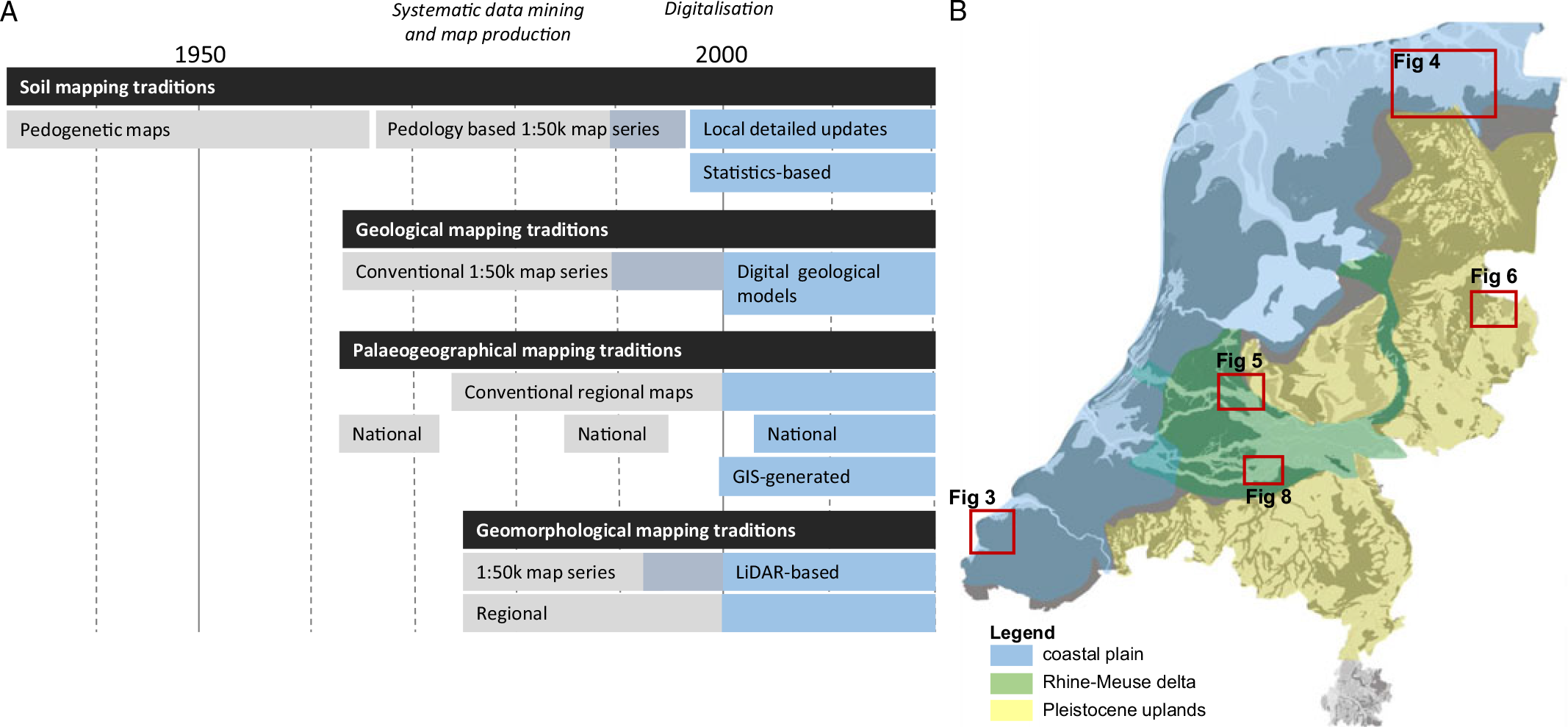

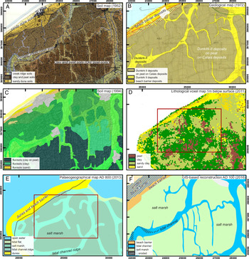


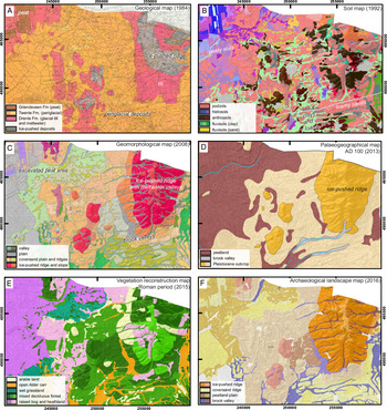
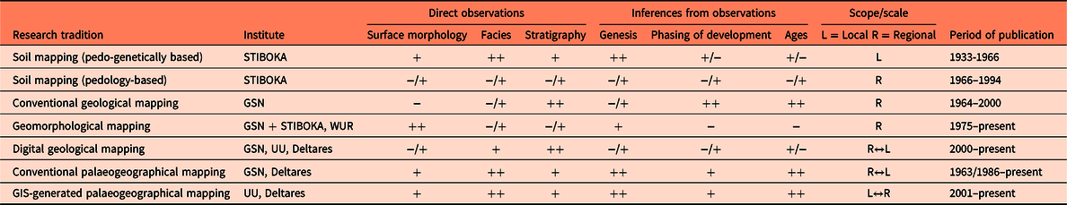


 Open access