

Introduction
Direct observations suggest that glaciers whose soles are at the melting point slide directly over their beds (e.g. Reference Kamb and LaChapelleKamb and LaChapelle, 1964; Reference PetersonPeterson, 1970; Reference BoultonBoulton and others, 1979; Reference VivianVivian, 1980), or that an equivalent subglacial motion takes place within an underlying layer of deforming sediment (Reference Boulton, Boulton, Morris, Armstrong and ThomasBoulton, 1979). Observations also suggest that in cold-based glaciers there is no such subglacial décollement, but that the glacier sole adheres to its bed (Reference GoldthwaitGoldthwait, 1960; Reference HoldsworthHoldsworth, 1974[b]). However, in this case an "apparent bed" may occur as a well-defined shear plane within the ice immediately above a basal boundary layer of ice (Reference HoldsworthHoldsworth, 1974[b]; Reference Boulton, Price and SugdenBoulton, 1972).
It is supposed that sliding or décollsment beneath temperate ice occurs because of the presence of a film of water between it and a bedrock surface, or because of high pore-water pressures in unlithified sediments which reduce their frictional resistance and allow them to deform. As yet, theories of basal ice movement have largely been developed from (Reference Weertman Weertman′s1957, Reference Weertman1964) model of temperate ice sliding over a bedrock surface (recently reviewed by Reference WeertmanWeertman, 1979; see also Reference LliboutryLliboutry, 1979).
The sliding law is a basal boundary condition for the large-scale bulk ice flow, and relates the tangential traction τb on a (smoothed-out) bed contour to the tangential velocity ub of the ice at this boundary in the same direction. Strictly τb and ub should be vectors in a tangent plane to allow a component of traction normal to the local sliding direction, but three-dimensional sliding theories tacitly assume that τb are ub are parallel. Negligible sliding velocity at this apparent bed, reflecting non-slip at the neighbouring real bed, must be a possible result.
The classical sliding theory introduced and extended by (Reference Weertman Weertman 1957, Reference Weertman1964) considers a bed consisting of a regular array of cuboidal objects with a bed roughness parameter defined by their size and spacing. Weertman derives a sliding velocity from the two components of regelation slip and plastic flow past the obstacles for a given basal shear stress. The resulting law has the form

where n is the exponent in the creep law deduced by Reference GlenGlen (1955) from uniaxial compression tests. Reference LliboutryLliboutry (1968) deduced a similar law but with disagreement over the appropriate measure of bed roughness and the magnitude of B. The form of the sliding law in Equation (1), with n = 1, has been supported by Reference NyeNye (1969) and Reference MorlandMorland (1976) for the Newtonian-fluid approximation, but the significant non-linear viscous response of ice defies similar treatment. The simplifications inherent in these formulations have, however, made it difficult to test the law in the field.
(Reference FowlerFowler 1979, Reference Fowler1981), in his analysis of sliding, defines two roughness parameters: the bed asperity σ, defined as the bed roughness wavelength [x] relative to ice depth d, and the bedrock roughness slope v defined as roughness amplitude [y] relative to wavelength [x]. He assumes a steady plane flow comprising an outer flow over the smoothed bed contour and an inner flow in a boundary layer on the scale of the roughness wavelength with perfect slip on the actual bed contour. The sliding velocity ub is both the velocity of the outer flow evaluated on the smoothed bed contour, and also the far-field velocity for the boundary-layer flow. Assuming a periodic bed contour and that ice satisfies Glen′s creep law, a singular perturbation analysis for σ « 1, with the further restriction v n+1 « 1, gives a lead-order relation

where R is an order-unity roughness parameter independent of σ. In Equation (2), both ub and τb are dimensionless variables, with respective units a longitudinal velocity magnitude and deviatoric stress magnitude in the outer flow. Note the power n in Equation (2) in contrast to ½(n+1) of Equation (1), and further that the Newtonian assumption (n = 1) of Reference NyeNye (1969) and Reference MorlandMorland (1976) cannot differentiate between either form.
Equation (2) can also be written
where d is the ice thickness, although Fowler′s analysis applies only to d >> [x], the bed roughness wavelength, so does not allow the limit d → 0. A simple extension of Equation (3) to allow variation of the thickness from its maximum magnitude in the central zone to zero at the margin is a separable relation

where the “friction parameter” λ depends on overburden depth d, or equivalently on the overburden pressure pb, and on the bed form and properties. The explicit function β in the second of Equations (4) with arbitrary exponent m is consistent with both Equations (1) and (3). Here we assert that the minimal ingredients of a sliding relation on the smoothed bed contour must be the tangential traction τb, the tangential velocity ub, and the overburden pressure pb. Ignoring dependence on pb, as in Equation (1) for example, leads to singular behaviour at a margin. The second of Equations (4) with different m and with creep described by a power law of exponent n (Reference GlenGlen, 1955), or a polynomial law (Reference Colbeck and EvansColbeck and Evans, 1973), has been applied by (Reference Morland and JohnsonMorland and Johnson 1980, Reference Morland and Johnson1982), hereafter abbreviated to MJ, and by Reference JohnsonJohnson (1981) to determine small-slope, steady ice-sheet profiles. A polynomial law has a finite non-zero gradient, that is bounded viscosity, as stress approaches zero, in contrast to the infinite viscosity of a power law with n > 1. In the following conclusions n = 1 refers to any smooth creep law with bounded viscosity. It was shown that bounded flows at the margins and ice divide, where the shear stress approaches zero, require

It was further noted (Reference Morland and JohnsonMorland and Johnson, 1982) that bounded longitudinal stress at the free surface requires n = 1. The optimum choice n = m = 1 corresponds to a bounded-viscosity creep law, such as a polynomial, and a sliding relation of the form of the second of Equations (4) which is linear in ub as ub → 0. The margin requirement that λ is linear in d as d → 0 is equivalent to linearity in pb, and supports the assertion that a sliding relation must depend on pb. In addition, the sliding relation is expected to depend on temperature, at least to distinguish temperate and cold basal conditions, but the present analysis does not account for temperature variation.
Our analysis comprises an inversion of the MJ steady, isothermal, plane-flow solution to determine ub, τb, and pb from given profile, bed, and surface accumulation/ablation area. Data from an individual ice sheet determine their distributions along the span and, subject to appropriate monotonicity properties, will determine one function of one variable in a connecting relation. Thus, even a separable two-function relation such as the first of Equations (4) cannot be determined, so an empirical sliding model must be restricted to a single-function form. We therefore adopt a relation of the form

with one arbitrary function λ (pb) to determine from individual ice-sheet data for different values of an integer exponent m. The correlation is carried out for two very different ice masses. First, the Expedition Glaciologique Internationale au Groenland (EGIG) profile of the present Greenland ice sheet (Reference Holtzscherer and BauerHoltzscherer and Bauer, [1956]; Reference HofmannHofmann, 1974). Secondly, the northwest profile of the Devon Island ice cap (Reference HyndmanHyndman, 1965; Reference MüllerMüller, 1977, p. 147–54), which is an order of magnitude smaller than the Greenland ice sheet. As expected, the magnitudes of the respective coefficients λ(pb) are very different, reflecting very different basal conditions. We suggest, though, that these two examples represent fairly extreme conditions, so that profile reconstructions using both relations would determine appropriate outer bounds. Naturally, the choice of m influences the pressure dependence of λ. We also find that there is no sensible β(ub) in the alternative single-function relation
which is consistent with the Greenland data. It is understood that our data correlation does not confirm a sliding relation of the form of Equation (6), but simply determines a basal boundary condition for the smoothed boundary of the global flow, which reconstructs the known profile from the given accumulation data.
It is known that significant temperature variation occurs in cold ice sheets, and that ice creep is significantly temperature-dependent in the relatively warm zones. The isothermal approximation allows only the specification of a constant temperature in the rate factor, and we recognize that a proper thermomechanical analysis could yield a different distribution of basal velocity, and hence correlate with different coefficients λ(pb). In particular, the calculated basal sliding velocity ub on the smoothed bed may well be reduced if enhanced velocity gradients in warmer zones increase the differential velocity between the surface and bed. Alternatively, if the enhancement occurs mainly in a thin thermal boundary layer below the adopted smooth bed, as proposed in Reference NyeNye′s (1959) pioneering ice-sheet analysis, then the basal sliding velocity so defined would be increased. We offer the present empirical models as the first quantitative correlation of a mechanical relation of the form of Equation (6) with global ice-sheet data, to be used for theoretical ice-sheet reconstructions until a sound thermomechanical theory is available.
Steady Isothermal Plane-Flow Theory
Plane flow with velocity components (u, v) in Oxy (Fig. 1) is assumed, where x, y are rectangular Cartesian axes with ox horizontal. The bed contour y = f(x) is restricted to small slope f ′ (x), and small mean bed inclination to the horizontal can be incorporated in the function f(x). The ice sheet has a free surface y = h(x), on which the normal and tangential tractions tn and ts are zero, and on which there is an accumulation distribution q defined as the volume flux of ice per unit horizontal cross-section entering the sheet. Negative q denotes ablation. Basal drainage b on y = f(x) is the volume flux of ice leaving the sheet per unit horizontal cross-section. Let qm denote a maximum accumulation (ablation) magnitude, and let h0 be a sheet thickness magnitude and ℓ0 a semi-span magnitude.
Ice-sheet cross-section.

We assume that the ice behaves like an incompressible non-linearly viscous fluid on gravity-driven-flow time scales, and satisfies a constitutive relation

where ![]() is the strain-rate tensor,
is the strain-rate tensor, ![]() is a dimensionless deviatoric stress tensor defined by
is a dimensionless deviatoric stress tensor defined by

with invariant
and where D0 and σ0 are strain-rate and stress units respectively and ![]() is the unit tensor. The temperature-dependent rate fa
is the unit tensor. The temperature-dependent rate fa
where
which is a close correlation constructed by Reference Smith and MorlandSmith and Morland (1981) to the Reference Mellor and TestaMellor and Testa (1969) uniaxial compression data at a uniaxial stress of 1.18 X 10⁶ N m–2 over the temperature range 212.15 K≤T≤ 273.15 K. The high stress level allows minimum (secondary) creep to be attained, and a common stress for all temperatures gives a direct measure of the temperature influence.
For the stress-dependent function ω(J2) we adopt a polynomial constructed by Reference Smith and MorlandSmith and Morland (1981) from Reference GlenGlen′s (1955) uniaxial compression data at T = 273.13 K, noting that a (273.13 K) is approximately unity for Equations (11) and (12). Following the MJ notation

with
when
The polynomial relation exhibits bounded viscosity at zero stress, unlike a power law with exponent n > 1, and correlates much closer to the same data (Reference Smith and MorlandSmith and Morland, 1981). Estimates of strain-rates from ice-shelf data (Reference ThomasThomas,1971, Reference Thomas1973; Reference HoldsworthHoldsworth, 1974 [a]) are considerably lower than the above laboratory rates at corresponding stresses. Since they are available only at a few particular stress levels, and hinge on flow solutions which ignore the significant temperature variation through the depth (Reference Morland and ShoemakerMorland and Shoemaker, 1982) we adopt the representation defined by Equations (13) to (15) and scale down the predicted strain-rates by appropriate choice of the constant temperature T in the isothermal theory. The magnitude of ω(J2) for deviatoric stress of order 105 N m–2, when J2 is order unity, is order unity.
The MJ solution is the lead-order approximation of a series solution in a small parameter ε which is a measure of the surface-slope magnitude. Expressions for the stress and velocities are derived in terms of the unknown profile h(x), which is then shown to satisfy a non-linear second-order ordinary differential equation subject to initial (margin) value and slope. The dimensionless normalized variables and analysis depend on ε which is determined by individual sheet conditions, but we wish to express the relations and solution in common normalized stress and velocity variables for application to any ice sheet. Accordingly, we start from the lead-order solution expressed in physical variables (Reference Morland and JohnsonMorland and Johnson, 1982), but without eliminating the basal velocity ub by the sliding law. That is

where

Note that τb denotes |σxy| and ub denotes |u| on the bed, equivalent to tangential components in the lead-order approximation for small bed slope, and u and σxy on y = f are positive (negative) when h′ is negative (positive). The profile equation is

where

subject to the margin conditions

where
The g 1, g definitions are more convenient than those of g, Ω in MJ which contain the rate factor a(T). Both g 1(t) and Ω(t) are order unity when t is order unity, corresponding to deviatoric stress of order 105 N m−2.
Now an order of magnitude for the basal shear stress τb is the stress unit σ0, 105 N m−2, while the magnitude of the basal pressure pb is greater by a factor ε−1, where ε is a surface-slope magnitude. Similarly, the normal velocity v has magnitude qm, while the longitudinal velocity is greater by a factor ε−1, which follows directly from the mass balance (MJ). We introduce common normalized variables in terms of a fixed slope magnitude
and depth and semi-span related by
so that h0 is determined directly ℓ0 is specified. Thus

and the dimensionless pressure ρ has a unit p0 = σ 0ε 0 −1, = 200 х 105 N m−2 with the values given in Equations (15) and (22). Choosing an accumulation and normal velocity magnitude
the dimensionless longitudinal velocity ū has a unit 200 m a−1.
In these dimensionless variables
where

depends on the value of h0 given by (23), that is, on the prescribed semi-span ℓ0. The profile equation becomes

with margin conditions

again depending on h0. We express the basal sliding Equation 6) in the form

where the required linear dependence of λ (Pb) as Pb → 0 is imposed by demanding that μ(p b) is analytic and bounded near p b = 0, with

so the coefficient of (Q0−B0) in the second margin condition (29) is simply
The MJ solution is obtained by applying a given sliding law (30) to eliminate μ b, and solving the consequent second-order non-linear ordinary differential equation(28), subject to initial conditions (29), for the profile H(X). Here we apply Equation(28) to a given profile H(X) with associated surface accumulation/ablation and basal drainage Q-B to evaluate μ b(X). With p b(X), τb(X) given by Equations (26) we can, in principle, determine one function λ(pb) in a sliding relation (30).
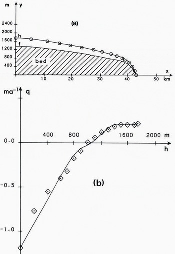
Greenland Ice Sheet Profile (EGIG)
In order to determine the basal (slip) velocity ūb from Equation (28) we need to know the surface profile H(X), the bed profile F(X) and the net accumulation/ablation distribution Q(H). We assume hence-forth that there is zero drainage at the bed, B = 0 in (28), since actual values are expected to be less than 0.01 m a−1 (Reference Boulton and RobinBoulton, 1983). The physical data for the surface and bed profile is taken from Reference HofmannHofmann (1974), with a corrected “near margin” profile from Reference Holtzscherer and BauerHoltzscherer and Bauer ([1956]). These data, along with a 7-degree Chebyshev polynomial approximation, appears in Figure 2a. The bed form for the EGIG profile is a series of undulations about sea-level, h = 0 (see e.g. Reference Boulton and RobinBoulton, 1983). We have investigated both this form and a flat bed at sea-level, obtaining similar global results. Detailed results based on the flat bed assumption are now presented. The accumulation/ablation data (Reference HofmannHofmann, 1974; personal communication from L.D. Williams in 1982) is shown in Figure 2b along with the corresponding 7-degree Chebyshev polynomial approximation.
-
(a) Greenland profile.
-
(b) Accumulation/ablation distribution. Continuous curves show Chebyshev polynomial approximations to the data points.

We choose ℓ0 be the actual distance between the divide and the margin which are then represented by end points (0, 1) in the dimensionless co-ordinate X. Here
The accumulation data give

instead of zero required by the steady-state comparison, but this value is extremely small in comparison with both the maximum normalized ablation value 3.75 and the maximum normalized accumulation value 0.52. A small adjustment to the data is therefore required to obtain a steady-state pattern; a convenient form is to replace Q(H) by QA(H) where

which can be interpreted as a small basal drainage component linearly dependent on altitude in Equation (28). If a function Q(X) is prescribed, then Equation (28) is directly integrable and an alternative adjustment

may be used. Both forms (34) and (35) were used in the numerical calculations and the results were indistinguishable. The results given in this section are based on the adjustment (34).
Using the polynomial representations of H(X) and QA(X), or Q A(X), the differential Equation 28) gives the dimensionless basal velocity μ b(X) displayed in Figure 3, along with the dimensionless pressure p b b and dimensionless shear traction τb given by Equation (26). Also shown is the normalized surface slope
Distributions of normalized basal pressure p
b, shear traction τb, tangential velocity ūb and surface slope determined by ![]() (Greenland profile). The three ūb curves correspond to T = −30°C (----), −26°C (——), −23°C (-.-.). The units of p
b, τb, ūb are respectively 200 × 105 N m−2, 105 N m−2, 200 m a−1.
(Greenland profile). The three ūb curves correspond to T = −30°C (----), −26°C (——), −23°C (-.-.). The units of p
b, τb, ūb are respectively 200 × 105 N m−2, 105 N m−2, 200 m a−1.

We now adopt the minimum temperature T = −30°C of the above set, which represents a natural bound of mean temperature, to produce the scaled-down strain-rates expected in natural ice flow as compared to laboratory creep tests (see earlier discussion on page 133). First we investigate the changes in the function λ(Pb) when different values of m are chosen in Equation (30). Figure 4 shows ub
1/m versus dimensionless slope τ
b/pb while Figure 5 shows the function ![]() versus p
b for m = 1,2,3,4. In both figures the results for m = 2,3,4 are not strongly dissimilar whereas the results for m = 1 have distinct features. In Figure 4 it is the behaviour of ūb
1/m as
versus p
b for m = 1,2,3,4. In both figures the results for m = 2,3,4 are not strongly dissimilar whereas the results for m = 1 have distinct features. In Figure 4 it is the behaviour of ūb
1/m as ![]() → 0, and in Figure 5 it is the behaviour
→ 0, and in Figure 5 it is the behaviour ![]() as p
b approaches its maximum value, both limits occurring at the ice divide. Both figures reflect the limit behaviour at the divide of
as p
b approaches its maximum value, both limits occurring at the ice divide. Both figures reflect the limit behaviour at the divide of ![]() approaching a non-zero finite value and
approaching a non-zero finite value and
 versus p
b is shown for different values of m in Figure 6. It is evident that μ(p
b is very closely linear, and with the same gradient, for each value of m including m = 1, until the basal pressure p
b reaches half its maximum value 1.3 which is attained at the divide. Thus is accurately represented by a quadratic over this range.
versus p
b is shown for different values of m in Figure 6. It is evident that μ(p
b is very closely linear, and with the same gradient, for each value of m including m = 1, until the basal pressure p
b reaches half its maximum value 1.3 which is attained at the divide. Thus is accurately represented by a quadratic over this range.
Variation of ūb
1/m with surface slope ![]() for different values of m (Greenland profile).
for different values of m (Greenland profile).

Sliding coefficient ![]() for m = 1 (——), m = 2 (---- ), m = 3 (-.-. ), ana m = 4 (-- --) (Greenland profile).
for m = 1 (——), m = 2 (---- ), m = 3 (-.-. ), ana m = 4 (-- --) (Greenland profile).

Reduced coefficient ![]() for m = 1 (——), m = 2 (---- ), m = 3 (-.-. ), and m = 4 (-- --) (Greenland profile).
for m = 1 (——), m = 2 (---- ), m = 3 (-.-. ), and m = 4 (-- --) (Greenland profile).

We now focus attention on the case m = 1, which guarantees a unique surface slope at the margin when ablation occurs there (Reference Morland and JohnsonMorland and Johnson, 1982). For convenient application of a sliding relation such as the second of Equations (30), we require an explicit representation of the function μ(p b over the entire range of p b. A linear form of μ(p b is assumed for 0 < p b < 0.7, while for 0.7 < p b < 1.3 a polynomial representation is used which satisfies continuity of μ, μ′, and μ" at p b = 0.7. Correlation by least squares is applied for increasing degree of polynomial until the resulting function is in good agreement with data, and not distinguishable in the graphical form on the scale of Figure 6. The result is

However, the continuation of this polynomial representation starts to decrease for p b > 1.49. Ice-sheet profiles generated with this sliding relation for which the pressure significantly exceeds this value so that μ returns to its low-pressure values would be physically unsatisfactory. Hence, beyond a pressure p m the polynomial form is replaced by a linear extension
which satisfies continuity of μ and μ′ at p b = p m. This latter transition value p m is arbitrary but it is chosen near the point of inflexion of the polynomial given by the second of Equations (36), i.e. the value of p at which the slope μ′(p b) starts to decrease.
The accuracy of the sliding-relation construction (36) can be verified by solving the ordinary differential Equation (28) for the EGIG profile H(X) with the given accumulation/ablation distribution shown in Figure 2b, with the adjustment (34). A graphical comparison with the original profile (Fig. 2a) shows no distinction. This applies to both Equations (36) and (36) amended by (37) since p b does not significantly exceed the transition pressure p m.
North-West Devon Island Ice Cap Profile
The procedure outlined in the previous section is now repeated for the much smaller north-west profile of the Devon Island ice cap. The surface profile data are extracted from Reference HyndmanHyndman (1965), which also contains estimates of the bed profile determined by gravity measurements for various cross-sections of the ice cap. Once again calculations are made for both a polynomial representation of the bed based on the available data, and on a simplified version (F varying linearly with H) which reflects similar global results. The results of the simplified version are presented.
The accumulation/ablation data for the north-west profile are taken from Reference MüllerMüller (1977 p. 147–54). A weighted mean of these data, which represent measurements for the years 1960 to 1975 inclusive, is determined in order to achieve an accumulation/ablation pattern which is as nearly as possible in steady state with the assumed profile. Although the margin of the ice cap is approximately 600 m above sea-level over the island, the accumulation/ablation data shown in Figure 7b is for altitudes ranging from the maximum value of 1800 m at the divide down to zero altitude. The lower-altitude data (h < 600 m) represent measurements on one of the outlet glaciers at the extreme north-west of the ice cap, an estimate of which must be included in the analysis in order to approximate a steady-state system. In Figure 7a the surface profile data for the ice cap and glacier are shown, along with the corresponding 11-degree Chebyshev polynomial representation and the simplified version of the bed profile (F = 7H/9) which reproduces measured depths near the summit (Reference Paterson and ClarkPaterson and Clarke, 1978).
-
(a) Devon Island profile.
-
(b) Aooumulation/ablation distribution. Continuous curves show Chebyshev polynomial approximations to the data points.
The span from ice cap divide to the glacier margin gives
A small adjustment of the form of Equation (34) is necessary in order to obtain a steady-state pattern, the value of the integral (33) here being 0.070 (as opposed to 0.009 for Greenland). Polynomial representations for h(x) and f(x) in Figure 7a and q(h) in Figure 7b, suitably normalized, are used in Equation (28) to determine μ
b(X). The distribution of velocity ūb, which now increases only to 13 m a–1 at the margin, basal pressure p
b and basal shear traction τb are shown in Figure 8, which also shows the variation of the surface slope ![]() with X. The calculations are again performed for the assumed uniform temperature T = –30°C.
with X. The calculations are again performed for the assumed uniform temperature T = –30°C.
Distributions of normalized basal pressure p
b, shear traction τb, tangential velocity ūb and surface slope determined by ![]() (Devon Island profile). The ūb curve corresponds to T = –30°C (---- ). The units of p
b, τb, ūb are respectively 200 × 105 N m–2, 105 N m–2, 200 m a–1.
(Devon Island profile). The ūb curve corresponds to T = –30°C (---- ). The units of p
b, τb, ūb are respectively 200 × 105 N m–2, 105 N m–2, 200 m a–1.

Figure 9 shows the behaviour of λ(pb) versus p
b for m = 1,2,3,4. Once again it is apparent that the case m = 1 is distinct from the cases m = 2,3,4 in the limiting behaviour of ![]() as both τb and ūb approach zero at the divide. Figure 10 shows μ(pb) versus p
b for m = 1,2,3,4. We note the similarity in shape with the corresponding curves in Figure 6, with each again having closely linear sections, but with a different gradient. The vast difference in the range of μ(pb) for the Greenland (Fig. 6) and Devon Island (Fig. 10) profiles is due mainly to the different scales of the basal pressure, p
b < 1.3 and p
b < 0.17 respectively, with the Greenland ice roughly eight times as thick as the Devon ice at corresponding values of distance X. An approximate smooth representation of μ(pb) for the m = 1 curve in Figure 10 is given by
as both τb and ūb approach zero at the divide. Figure 10 shows μ(pb) versus p
b for m = 1,2,3,4. We note the similarity in shape with the corresponding curves in Figure 6, with each again having closely linear sections, but with a different gradient. The vast difference in the range of μ(pb) for the Greenland (Fig. 6) and Devon Island (Fig. 10) profiles is due mainly to the different scales of the basal pressure, p
b < 1.3 and p
b < 0.17 respectively, with the Greenland ice roughly eight times as thick as the Devon ice at corresponding values of distance X. An approximate smooth representation of μ(pb) for the m = 1 curve in Figure 10 is given by
Sliding coefficient ![]() for m = 1 (——), m = 2 (----), m = 3 (-.-. ), and m = 4 (-- --) (Devon Island profile).
for m = 1 (——), m = 2 (----), m = 3 (-.-. ), and m = 4 (-- --) (Devon Island profile).

Reduced coefficient ![]() for m = 1 (——), m = 2 (---- ), m = 3 (-.-. ), and m = 4 (-- -- ) (Devon Island profile).
for m = 1 (——), m = 2 (---- ), m = 3 (-.-. ), and m = 4 (-- -- ) (Devon Island profile).

Discussion of Results
The steady-state isothermal solution of Reference Morland and JohnsonMorland and Johnson (1980, Reference Morland and Johnson1982), with different normalization, has been used to determine the basal tangential veloQ city ūb on a smooth bed contour defining the lower boundary for the global flow. Calculations were made using the surface profile data and accumulation/ablation data from two very different examples of present-day ice masses, namely the Greenland ice sheet and the Devon Island ice cap. Normalized distributions of the basal pressure p b, the basal tangential traction τb and the basal tangential velocity ūbwere determined, and used to find a “friction” parameter λ(pb) in an assumed sliding relation of the form of Equation (30) for m = 1,2,3, and 4.
It is found for each case that the behaviour of ![]() for m = 2,3, and 4 is similar but that the m = 1 results are distinct. This phenomenon stems from the limiting value of
for m = 2,3, and 4 is similar but that the m = 1 results are distinct. This phenomenon stems from the limiting value of ![]() as both τb and ūb approach zero at the divide. For m = 1, the limit is finite and non-zero, while for m > 1, the limit is zero. These differences are evident in Figures 4, 5, and 9.
as both τb and ūb approach zero at the divide. For m = 1, the limit is finite and non-zero, while for m > 1, the limit is zero. These differences are evident in Figures 4, 5, and 9.
In general, initially decreases from a finite positive value as p
bincreases from zero then starts to increase from a mid-range value p
t of p
b (see Figs 6 and 10). The main differences between the two examples are
-
(i) for the Greenland profile λ(pb) is a monotonic function of p b, while for the Devon Island ice cap it is not;
-
(ii) the much smaller range of the Devon Island ice cap basal pressure leads to dramatically larger values of μ(pb).
Such wide differences in magnitude of the function μ, and hence λ in Equation (6), correspond to wide differences in the calculated basal sliding velocity at given basal shear stress. Bed structure and thermal conditions will influence the gross friction represented by the sliding law, but more significantly, bed mobility could significantly reduce the actual sliding velocity. Whereas it is the absolute basal ice velocity which appears in the differential Equation (28), it is strictly the relative slip velocity which should enter the sliding relations (4), (6), and (7). Compatibility of the predicted Greenland and Devon basal velocity magnitudes, which approach 130 m a–1 and 13 m a–1 at the respective margins, in the common range of overburden pressure could require, though, a significant Greenland bed movement to account for such a large fraction of the calculated basal velocity.
Significant temperature profiles and strong creep dependence on temperature through a(T) will influence the basal velocity calculation, and basal temperature could affect the sliding “friction” or influence bed mobility. Given an empirically deduced temperature field, it is possible to generalize the analysis to incorporate the rate factor a[T(x, y)], and we are now investigating such temperature effects on the basal velocity.
In principle, given ice-sheet data could be correlated to other forms of sliding relations: for example, the form of the first of Equations (4) with λ(Pb) prescribed and β(ub) determined. More specifically, if we choose Equation (7) which satisfies the required asymptotic behaviour (5) as pb → 0, then β(ub) = τb/pb determined by the Greenland data is represented in the normalized variables ūb, p
b, τb by the curve for m = 1 in Figure 4. Note, however, the large gradient of the corresponding ![]() when
when ![]() is near unity, which is associated with the rapid change of the sliding velocity ūb while the surface slope changes little. That is, the sliding velocity is very sensitive to small changes of surface slope, and it would be difficult to represent the function β–1 accurately.
is near unity, which is associated with the rapid change of the sliding velocity ūb while the surface slope changes little. That is, the sliding velocity is very sensitive to small changes of surface slope, and it would be difficult to represent the function β–1 accurately.
Unfortunately, data from a small set of ice sheets cannot determine a function of two variables such as τb(Pb, ub), so we must start with restricted forms such as Equation (6), or Equation (6) extended to include a temperature-dependent factor. It is clear that there is no universal sliding law, and choice of a basal sliding condition will depend on the particular application. Until thermal and bed-structure effects are established, a range of sliding conditions should be considered to estimate their influence on solutions. Such a parameter study has been included in an investigation of equilibrium profiles in various environments by Reference Boulton, Boulton, Smith and MorlandBoulton and others (1984).
Acknowledgement
This work was supported by a United Kingdom Natural Environment Research Council Grant GR3/4114: Relationship between glaciers and climate during the last glacial period in north-west Europe.


