1 Time-varying coefficient modeling as tools to examine differences in associations across time

TVCM is a flexible approach for studying how associations between variables evolve over time. Rather than imposing a predefined form of change, TVCM can capture complex, nonlinear patterns as a function of continuous time. Graphical displays of these patterns help characterize how change unfolds and pinpoint periods when relationships among variables are strongest or weakest, offering valuable insights into critical windows for intervention, among other things (Lanza & Linden-Carmichael, Reference Lanza and Linden-Carmichael2021; Tan et al., Reference Tan, Shiyko, Li, Li and Dierker2012). In its original form, TVCM poses an extension of linear regression. To illustrate, let $x_{it}$ and $y_{it}$ denote values on two variables of interest, reported by individual $i \in \{1, \ldots , N\}$ at time t after the start of an EMA. In a typical TVEM setup, both the intercept $\beta _0(t)$ and the regression coefficient $\beta _1(t)$ are allowed to change over time, while the residual standard deviation $\sigma $ is assumed constant. This can be written as

(1) $$ \begin{align} y_{it} \sim \mathcal{N} \left(\beta_0(t) + \beta_1(t) x_{it}, \sigma\right). \end{align} $$

In TVCM, the aim is to obtain smooth coefficient functions of the regression parameters of interest over the interval $[l,u]$ . The interval $[l,u]$ can represent time in different ways depending on the application. It may correspond to the same real-time period for all participants (e.g., the first weeks of a semester in a student sample), or it may represent participant-specific segments of time (e.g., the first weeks following a cessation attempt in an addiction study). What is crucial is that the time variable is meaningful with respect to the phenomenon under study—not merely the arbitrary span of an EMA—and that the time scale is aligned across participants with respect to shared reference event (see Singer & Willett, Reference Singer and Willett2003, for further discussions on how to conceptualize time in the analysis of longitudinal data).

To capture smooth coefficient functions of arbitrary form, TVCM draws on splines. In what follows, we focus on truncated power splines, in which the interval $[l,u]$ is divided into $K+1$ subintervals:

$$\begin{align*}[\tau_0, \tau_1), \; [\tau_1, \tau_2), \; \ldots, \; [\tau_{K-1}, \tau_K), \; [\tau_K, \tau_{K+1}]. \end{align*}$$

The subintervals are defined by K knots $\{\tau _1, \tau _2, \ldots , \tau _K\}$ , typically equally spaced, with

$$\begin{align*}l = \tau_0 < \tau_1 < \cdots < \tau_K < \tau_{K+1} = u. \end{align*}$$

Then, the coefficient function is approximated piecewise by lower-order polynomials over each subinterval, connected by the K knots.

For concreteness, we focus on the time-varying regression coefficient from Equation (1). Using piecewise quadratic functions, the coefficient function $\beta _1(t)$ can be approximated by a linear combination of a quadratic base function and K truncated power functions:

(2) $$ \begin{align} \beta_{1}(t) &= \underbrace{d_{0} + d_{1}t + d_{2}t^2 \vphantom{\sum_{k=1}^{K}}}_{\text{quadratic base function}} + \underbrace{\sum_{k=1}^{K} d_{2+k}(t-\tau_k)^2_+}_{\text{truncated power functions}},\\ \text{where } & (t-\tau_k)^2_+ = \begin{cases} 0, & \text{if } t \leq \tau_k, \\ (t-\tau_k)^2, & \text{if } t> \tau_k. \notag \end{cases} \end{align} $$

Note that the parameters defining the coefficient functions are not directly interpretable. Instead, results are interpreted visually through graphical displays of the implied coefficient functions across the interval bounded by l and u.

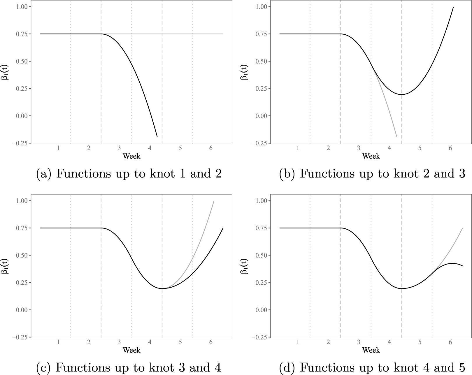
To illustrate, Figure 1 shows how a hypothetical coefficient function is built successively. In each panel, the curve implied by the linear combination of the base function and the truncated power functions up to knot j

$$\begin{align*}d_{0} + d_{1}t + d_{2}t^2 + \sum_{k=1}^{j} d_{2+k}(t-\tau_k)^2_+ \end{align*}$$

is shown in black, while the corresponding curve up to knot $j-1$ is shown in gray. This visualization demonstrates how each truncated power function modulates the coefficient function within its corresponding subinterval.

Figure 1

Illustration of a successfully built hypothetical coefficient function. Each panel compares the function up to knot j (in black) against the function up to knot $j-1$ (in gray).

Figure 1 Long description

Four panels labeled a through d. Each panel shares a common x-axis labeled Week from 0 to 6 and a y-axis labeled beta sub 1 (t) from negative 0.25 to 1.00. Vertical dashed and dotted lines represent knot locations.

* Panel a. Functions up to knot 1 and 2. A gray horizontal line remains constant at 0.75. A black line follows this until week 2.5, then curves downward sharply toward negative 0.25 by week 4.

* Panel b. Functions up to knot 2 and 3. The gray line follows the curve from panel a. The black line diverges at week 3.5, forming a trough at week 4.5 before curving upward toward 1.00 at week 6.

* Panel c. Functions up to knot 3 and 4. The gray line follows the upward curve from panel b. The black line diverges at week 4.5, maintaining a lower trajectory that ends at 0.75 at week 6.

* Panel d. Functions up to knot 4 and 5. The gray line follows the trajectory from panel c. The black line diverges at week 5.5, curving downward to end at approximately 0.40 at week 6.

For ease of interpretation, let us imagine that the depicted coefficient function represents the time-varying regression coefficient for nervousness and threat monitoring across a six-week interval (i.e., the effect of nervousness on threat monitoring), spanning the two weeks before, during, and after an intensive therapy targeting anxiety patients. Five knots $\tau _k$ , marked with vertical lines, are placed at weekly intervals, with knots $\tau _2 = 2$ and $\tau _4 = 4$ , depicted with dashed lines, marking the start and end of therapy, respectively.

We start with a linear base function ( $d_0 = 0.75$ and $d_1 = d_2 = 0$ ). This base function determines the hypothetical coefficient function in the first segment of Figure 1, capturing an initially stable association between nervousness and threat monitoring in Week 1. The relationship also remains stable throughout the second segment, when considering the function up to the first knot, as reflected by $d_3 = 0$ . In Week 3, with the second knot, which coincides with the onset of therapy two weeks into the EMA, the relationship begins to weaken ( $d_4 = -0.4$ ; see the third segment in Figure 1a). In Week 4, with the third knot, the decline is dampened ( $d_5 = 0.8$ ). The association continues to weaken but at a slower rate than implied by the coefficient function up to knot 2 (compare the gray and black lines in the fourth segment of Figure 1b). Then, in Week 5, after the end of therapy, the relationship starts to strengthen again, but at a slower rate than implied by the coefficient function up to knot 3 ( $d_6 = -0.2$ ; compare the gray and black lines in the fifth segment of Figure 1c). Finally, in Week 6, the association flattens out ( $d_7 = -0.5$ ; Figure 1d).

2 Running example: Nervousness and threat monitoring across the course of therapy

To illustrate and study our TVCM developments, we make use of intensive longitudinal data from 16 patientsFootnote ¹ with mixed anxiety disorders who received a group-based attention training technique intervention over a two-week period (see Snuggerud et al., Reference Snuggerud, Nordahl, Vrabel, Hoffart and Johnson2026a, for further details). Ethical approval was obtained from the Norwegian Ethical Committee (REK/2021/269896). Data on multiple emotional states, metacognitive strategies, and metacognitive beliefs were collected over six weeks using EMA: two weeks before treatment, two weeks during treatment, and two weeks after treatment, creating a natural timeline with respect to shared reference events. Participants completed assessments daily at fixed time points (8.00 am, 12.00 pm, 4.00 pm, and 8.00 pm), and contributed a median of 147 available measurement occasions (range: 99–172).

Note that despite repeated calls to complement or even substitute traditional methods for evaluating clinical interventions with EMA (Mofsen et al., Reference Mofsen, Rodebaugh, Nicol, Depp, Miller and Lenze2019; Moore et al., Reference Moore, Depp, Wetherell and Lenze2016; Targum et al., Reference Targum, Sauder, Evans, Saber and Harvey2021; Webb et al., Reference Webb, Hilt, Swords, Bolt, Fisher and Goldberg2025), fine-grained tracking of patients via EMA across the entire intervention period, including pre- and post-intervention baseline and follow-up periods, is still relatively rare in clinical intervention research. The present data therefore offer a rare opportunity to examine the dynamic nature of change during the intervention in detail, and to assess whether and how such changes are subsequently sustained. Notwithstanding the limited sample size, the data afford unusually rich temporal information, with the number of measurement occasions far exceeding what is typical in EMA studies (i.e., on average six assessments per day over seven days; Wrzus & Neubauer, Reference Wrzus and Neubauer2023). Because the accuracy of TVCM results crucially depends on the number of measurement occasions rather than the sample size—as demonstrated in applications with $N=1$ designs (Bringmann et al., Reference Bringmann, Hamaker, Vigo, Aubert, Borsboom and Tuerlinckx2017)—our example data set is particularly well suited for illustrating TVCM developments.

Among the assessed emotional states, metacognitive strategies, and metacognitive beliefs, we focus on nervousness and threat monitoring as two illustrative phenomena of interest and apply the proposed TVCM developments to investigate between-person differences in how their levels, variability, and coupling evolved over the period from two weeks before to two weeks after intensive therapy. Both constructs were assessed at each EMA prompt with the items “Right now, I feel nervous” (Norwegian original: “Akkurat nå føler jeg meg nervøs”) and “Right now, I am scanning for potential threats” (“Akkurat nå ser jeg etter farer”), using a visual analog scale from 0 (“not at all”) to 100 (“completely”). To facilitate model estimation, we rescaled the time scale by setting $l=0$ to denote the onset of EMA data collection for each participant and $u=1$ to denote the maximum amount of time elapsed between the onset and the final EMA measurement. Both item scores were rescaled to the unit interval by dividing by 100.

3 Model 1: A time-varying coefficient formulation of the multivariate normal distribution

To interpret standard TVCM regression parameters meaningfully, well-defined assumptions about the directional relationships between constructs are required. As noted above, however, researchers may not always have or do not want to incorporate such assumptions in their analyses. In addition, they may be interested in studying phenomena going above and beyond mean levels and associations. In the present study, we, therefore, aim to broaden TVCM beyond regression-based applications to capture not only mean levels and directed associations, but also changes in variability and co-occurrence over time.

We start with a customary, aggregate-level TVCM formulation of the multivariate normal distribution. We first introduce the model and then discuss its implementation and illustrative empirical results. For simplicity, we consider two variables, $x_{it}$ and $y_{it}$ , and assume that they are bivariate normally distributed. In our model, all parameters defining the bivariate normal distribution—the mean vector, standard deviations, and the correlation—are allowed to vary as a function of time, that is,

(3) $$ \begin{align} \begin{bmatrix} x_{it}\\ y_{it} \end{bmatrix} & \sim \mathcal{N}_2\left(\boldsymbol{\mu}(t), \boldsymbol{\Sigma}(t) \right),\\[-3pt] \text{where } & \boldsymbol{\mu}(t) = \begin{bmatrix} \mu_{x}(t)\\ \mu_{y}(t) \end{bmatrix} \quad \text{and} \quad \boldsymbol{\Sigma}(t) = \begin{bmatrix} \sigma_{x}^2(t) & \rho_{xy}(t) \sigma_{x}(t)\sigma_{y}(t) \\ \rho_{xy}(t) \sigma_{x}(t)\sigma_{y}(t) & \sigma_{y}^2(t) \end{bmatrix}. \notag \end{align} $$

Defining knots and subintervals as above, we approximate the smooth coefficient functions of these parameters over the interval $[l, u]$ by

(4) $$ \begin{align} \mu_{x}(t) &= a_{x0} + a_{x1}t + a_{x2}t^2 + \sum_{k=1}^{K} a_{x,2+k}(t-\tau_k)^2_+ \\[-3pt] \mu_{y}(t) &= a_{y0} + a_{y1}t + a_{y2}t^2 + \sum_{k=1}^{K} a_{y,2+k}(t-\tau_k)^2_+ \notag \\[-3pt] \sigma_{x}(t) &= \exp\left(b_{x0}+b_{x1}t + b_{x2}t^2 + \sum_{k=1}^{K} b_{x,2+k}(t-\tau_k)^2_+\right) \notag \\[-3pt] \sigma_{y}(t) &= \exp\left(b_{y0}+b_{y1}t + b_{y2}t^2 + \sum_{k=1}^{K} b_{y,2+k}(t-\tau_k)^2_+\right) \notag \\[-3pt] \rho_{xy}(t)& = \text{tanh}\left( c_{0} + c_{1}t + c_{2}t^2 + \sum_{k=1}^{K} c_{2+k}(t-\tau_k)^2_+\right), \notag\\[-3pt] \text{where } & (t-\tau_k)^2_+ = \begin{cases} 0, & \text{if } t \leq \tau_k, \notag \\[-3pt] (t-\tau_k)^2, & \text{if } t> \tau_k. \end{cases} \notag \end{align} $$

Note that for standard deviations and the correlation coefficient, coefficient functions refer to log-transformed and Fisher z-transformed parameters, respectively. The inverse transformations are given by $\exp (\cdot )$ for standard deviations and $\tanh (\cdot )$ for the correlation coefficient. These transformations ensure that the respective coefficients remain within their admissible parameter space, namely, $\sigma _{x}(t)>0$ , $\sigma _{y}(t)>0$ , and $-1 < \rho _{xy}(t) < 1$ .Footnote ²

3.1 Prior settings and model implementation

In our Bayesian implementation, we use diffuse normal priors with mean 0 and standard deviation 10 for the polynomial base term parameters ( $a_{x0}, a_{x1}, a_{x2}, a_{y0}, \ldots , c_1, c_2$ ). To smooth the coefficient functions and avoid overfitting, the truncated power basis parameters ( $a_{x,2+1}, a_{x,2+2}, \ldots c_{2+K-1}, c_{2+K}$ ) are equipped with hierarchical priors (as in Tan et al., Reference Tan, Shiyko, Li, Li and Dierker2012), that is,

(5) $$ \begin{align} a_{x,2+k} & \sim \mathcal{N}(0,\eta_{ax}) \\ a_{y,2+k} & \sim \mathcal{N}(0,\eta_{ay}) \notag\\ b_{x,2+k} & \sim \mathcal{N}(0,\eta_{bx}) \notag\\ b_{y,2+k} & \sim \mathcal{N}(0,\eta_{by}) \notag\\ c_{2+k} & \sim \mathcal{N}(0,\eta_{c}) \quad \text{for } k = 1, 2, \ldots, K. \notag \end{align} $$

We use half-Cauchy priors with location 0 and scale 2 for the hyperparameters ( $\eta _{ax}, \eta _{ay}, \ldots , \eta _c$ ) of these hierarchical priors.

For all model illustrations, we set $K=7$ , with five knots evenly spaced over the interval $[l=0,u=1]$ , and two additional knots placed during therapy to increase the sensitivity of the coefficient functions in this period of expected rapid change. We used Stan version 2.19 (Stan Development Team, 2017) with the rstan package version 2.19.3 (Guo et al., Reference Guo, Gabry and Goodrich2018) to obtain the Bayesian parameter estimates. For each model, we ran two Markov chain Monte Carlo (MCMC) chains with 10,000 iterations each, with the first half being employed as warm-up. The sampling procedure was assessed on the basis of potential scale reduction factor (PSRF) values, with PSRF values below 1.10 for all parameters being considered as satisfactory (Gelman & Rubin, Reference Gelman and Rubin1992; Gelman & Shirley, Reference Gelman, Shirley, Brooks, Gelman, Jones and Meng2011). We did not observe PSRF values exceeding 1.10 for any of the estimated models. We employed the posterior mean (EAP) as a Bayesian point estimate for each parameter constituting the coefficient functions. All analyses were conducted in R version 4.4.3 (R Development Core Team, 2017).

3.2 Results

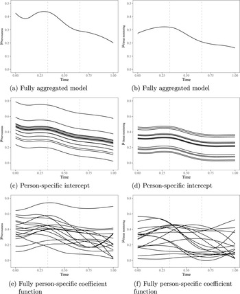
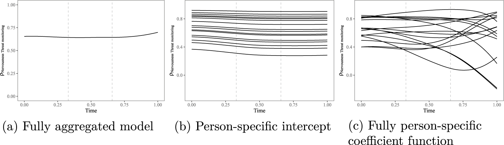
Figures 2a, 2b, 3a, 3b, and 4a show the time-varying means, standard deviations, and correlations of nervousness and threat monitoring obtained from the TVCM formulation of the bivariate normal distribution, which remains fully aggregated, that is, yields average parameters across persons. The dashed vertical lines indicate the approximate start and end of therapy. Note that the timing of therapy was not incorporated in the models but is included in the figure to aid interpretation.

Figure 2

Time-varying means of nervousness (left column) and threat monitoring (right column) for different modeling approaches. Note that y-axes for the fully aggregated results and individual-specific trajectories differ in scale.

Figure 2 Long description

A grid of six line graphs arranged in two columns and three rows. The left column displays mu sub Nervousness and the right column displays mu sub Threat monitoring. All graphs share an x-axis for Time ranging from 0.00 to 1.00 with vertical dashed lines at approximately 0.33 and 0.66.

* Top row (a and b) Fully aggregated model: The y-axis ranges from 0.0 to 0.5. Panel a shows nervousness peaking at 0.33 before a steady decline. Panel b shows threat monitoring peaking slightly before 0.33 followed by a gradual decline.

* Middle row (c and d) Person-specific intercept: The y-axis ranges from 0.0 to 0.8. Both panels show a series of parallel curves representing individual trajectories. In panel c, the curves show a slight initial peak then a downward trend. In panel d, the curves show a subtle wave pattern with a general decline after the second dashed line.

* Bottom row (e and f) Fully person-specific coefficient function: The y-axis ranges from 0.0 to 0.8. These panels show highly variable, intersecting individual curves. Panel e shows diverse nervousness trajectories with some increasing and others decreasing sharply. Panel f shows complex, oscillating threat monitoring paths that cross one another frequently throughout the time period.

Figure 3

Time-varying standard deviations of nervousness (left column) and threat monitoring (right column) for different modeling approaches. Note that y-axes for the fully aggregated results and individual-specific trajectories differ in scale.

Figure 3 Long description

The figure consists of six line graphs arranged in a 3 by 2 grid. All graphs share an x-axis labeled Time, ranging from 0.00 to 1.00, with vertical dashed lines at approximately 0.33 and 0.66.

Top Row: Fully aggregated model.

Panel a (left) shows sigma Nervousness on a y-axis from 0.10 to 0.35. A single curve starts at 0.28, peaks slightly, then follows a sigmoid decline to 0.21.

Panel b (right) shows sigma Threat monitoring on the same scale. The curve mirrors panel a, starting at 0.26, peaking at 0.25 time, and declining to 0.19.

Middle Row: Person-specific intercept.

Panel c (left) shows sigma Nervousness on a y-axis from 0.0 to 0.5. It contains approximately 20 individual curves that follow a parallel downward trend, ranging from 0.18 to 0.45 at time 0.

Panel d (right) shows sigma Threat monitoring on the same scale. The curves are mostly parallel with a slight dip and recovery, clustered tightly between 0.15 and 0.25, with a few outliers above and below.

Bottom Row: Fully person-specific coefficient function.

Panel e (left) shows sigma Nervousness on a y-axis from 0.0 to 0.5. The curves are no longer parallel, showing intersecting trajectories that generally trend downward but with varying slopes and curvatures.

Panel f (right) shows sigma Threat monitoring on the same scale. The curves show high variability and frequent intersections, with some trajectories rising sharply toward time 1.00 while others decline or remain flat.

Figure 4

Time-varying correlations of nervousness and threat monitoring for different modeling approaches. Note that y-axes for the fully aggregated results and individual-specific trajectories differ in scale.

Figure 4 Long description

A multi-panel figure containing three line graphs labeled a, b, and c. All graphs share a horizontal x-axis for Time ranging from 0.00 to 1.00 and a vertical y-axis for rho nervousness threat monitoring. Two vertical dashed gray lines intersect the x-axis at approximately 0.33 and 0.66 in all panels.

* Panel a, Fully aggregated model. The y-axis ranges from 0.00 to 1.00. A single solid black line remains relatively flat at a correlation of approximately 0.65, with a slight upward curve toward the end of the time period.

* Panel b, Person-specific intercept. The y-axis ranges from 0.0 to 0.8. The graph displays approximately 20 parallel or near-parallel horizontal lines stacked vertically. These lines represent individual trajectories that maintain a constant offset from one another, ranging from a correlation of 0.3 to 0.9.

* Panel c, Fully person-specific coefficient function. The y-axis ranges from 0.0 to 0.8. The graph shows approximately 20 highly variable and intersecting lines. While some lines remain stable, others show significant fluctuations, including steep declines toward a 0.0 correlation or sharp peaks, indicating high individual variability in the correlation over time.

The mean level of nervousness (Figure 2a) showed a slight increase in the week preceding therapy onset, possibly indicative of anticipatory arousal, while threat monitoring (Figure 2b) remained stable over the same period. With the start of therapy, both constructs showed steady decline, somewhat more pronounced for nervousness than for threat monitoring. Both trajectories flattened out during the two-week follow-up period. A similar pattern was observed for the standard deviation of threat monitoring (Figure 3b), which exhibited a steady, substantial decline following the onset of therapy. Nervousness, in contrast, exhibited a somewhat less pronounced reduction in variability (Figure 3a). To evaluate whether model-implied coefficients at the approximate start of therapy were credibly different from those at therapy end, we obtained their difference as derived parameters. Mean levels of nervousness and threat monitoring were both credibly higher at the start than at the end of therapy (differences of 0.14, 95% credibility interval: [0.11, 0.18], and 0.11 [0.08, 0.15], respectively), as were their standard deviations (0.04 [0.02, 0.06] and 0.06 [0.04, 0.09], respectively).

In sum, the intensive therapy appears to have produced sustained reductions in both average levels and volatility of nervousness and threat monitoring, with declines beginning right from the onset. For threat monitoring, reductions in variability were more pronounced and closely paralleled the decline in average levels, whereas for nervousness, reductions in mean levels were more pronounced while accompanying decreases in variability were comparatively modest. In contrast, the coupling between nervousness and threat monitoring appeared unaffected by the intensive therapy, as indicated by a correlation coefficient remaining stable at approximately 0.65 throughout the study period (Figure 4a) and a difference in coefficients between therapy start and end of 0.00 [ $-$ 0.05; 0.06].Footnote ³

4 Model 2: A hierarchical extension with person-specific coefficient intercepts

In its original form, TVCM supports investigating aggregate effects but does not support conclusions about how change unfolds at the level of individual participants (Piccirillo & Foster, Reference Piccirillo and Foster2023). Yet, arguably, this is precisely the focus of many research questions addressed with intensive longitudinal data (e.g., Hamaker, Reference Hamaker2025; Laurenceau et al., Reference Laurenceau, DiGiovanni and Bolger2025). Furthermore, both the original regression-based TVCM variant (Equation (1)) and its multivariate normal counterpart introduced above (Equation (3)) neglect the nested structure of intensive longitudinal data from multiple participants—a limitation frequently acknowledged in both methodological and applied TVCM studies (e.g., Tan et al., Reference Tan, Shiyko, Li, Li and Dierker2012; Wright et al., Reference Wright, Hallquist, Swartz, Frank and Cyranowski2014).

Both issues can be addressed by integrating TVCM with hierarchical modeling approaches (Shim et al., Reference Shim, Sohn and Hwang2017; Sørensen & McCormick, Reference Sørensen and McCormick2025; Sun et al., Reference Sun, Zhang and Tong2007; Tan et al., Reference Tan, Shiyko, Li, Li and Dierker2012), a strategy we also adopt in our TVCM formulation of the multivariate normal distribution to investigate interindividual differences beyond aggregate trajectories. The simplest extension that already allows for some degree of heterogeneity in coefficient functions is the introduction of a person-specific intercept term to the polynomial base function (as done in, e.g., Shim et al., Reference Shim, Sohn and Hwang2017, Sun et al., Reference Sun, Zhang and Tong2007, and Tan et al., Reference Tan, Shiyko, Li, Li and Dierker2012). This approach accounts for interindividual differences in the initial strength of the parameter of interest at the onset of the EMA period. It, however, rests on the assumption that trajectories of untransformed coefficient functions (i.e., prior to applying the exponential or tanh transformation for standard deviations and correlations) run in parallel across time:

(6) $$ \begin{align} \mu_{i,x}(t) & = a_{i,x0} + a_{x1}t + a_{x2}t^2 + \sum_{k=1}^{K} a_{x,2+k}(t-\tau_k)^2_+\\ \mu_{i,y}(t) & = a_{i,y0} + a_{y1}t + a_{y2}t^2 + \sum_{k=1}^{K} a_{y,2+k}(t-\tau_k)^2_+ \notag \\ \sigma_{i,x}(t) &= \exp\left(b_{i,x0}+b_{x1}t + b_{x2}t^2 + \sum_{k=1}^{K} b_{x,2+k}(t-\tau_k)^2_+\right) \notag \\ \sigma_{i,y}(t) &= \exp\left(b_{i,y0}+b_{y1}t + b_{y2}t^2 + \sum_{k=1}^{K} b_{y,2+k}(t-\tau_k)^2_+\right) \notag \\ \rho_{i,xy}(t)& = \text{tanh}\left( c_{i0} + c_{1}t + c_{2}t^2 + \sum_{k=1}^{K} c_{2+k}(t-\tau_k)^2_+\right).\notag \end{align} $$

Note the introduction of the subscript i to the time-varying parameters ( $\mu _{i,x}(t),\mu _{i,y}(t), \ldots , \rho _{i,xy}(t)$ ) and the intercept parameters of the coefficient functions ( $a_{i,x0}, a_{i,y0}, \ldots , c_{i0}$ ).

Introducing a person-specific intercept into the time-varying coefficient functions enables the identification, quantification, and illustration of between-person heterogeneity in initial coefficient levels, for example, via the standard deviations of the person-specific intercepts or by showing exemplar coefficient functions for individuals with low, medium, and high values.

4.1 Prior settings

For the individual-specific intercepts, we use hierarchical priors, that is,

(7) $$ \begin{align} a_{i,x0} & \sim \mathcal{N}(\nu_{ax0}, \phi_{ax0})\\ a_{i,y0} & \sim \mathcal{N}(\nu_{ay0}, \phi_{ay0}) \notag\\ b_{i,x0} & \sim \mathcal{N}(\nu_{bx0}, \phi_{bx0}) \notag\\ b_{i,y0} & \sim \mathcal{N}(\nu_{by0}, \phi_{by0})\notag\\ c_{i0} & \sim \mathcal{N}(\nu_{c0}, \phi_{c0}).\notag \end{align} $$

The group-level means of the person-specific coefficient intercepts ( $\nu _{ax0}, \nu _{ay0}, \ldots , \nu _{c0}$ ) are assigned a normal prior with mean $0$ and standard deviation $10$ , and the group-level standard deviations ( $\phi _{ax0},\phi _{ay0}, \ldots , \phi _{c0}$ ) are assigned a half-Cauchy prior with location 0 and scale 2. Priors for the remaining parameters are identical to those specified for the fully aggregated model.

5 Model 3: A hierarchical extension with fully person-specific coefficient functions

To relax the assumption that the shapes of coefficient trajectories are shared among individuals and only differ in their level, all components of the time-varying coefficient function can be allowed to be person-specific (as in Sørensen and McCormick, Reference Sørensen and McCormick2025), that is,

(8) $$ \begin{align} \mu_{i,x}(t) & = a_{i,x0} + a_{i,x1}t + a_{i,x2}t^2 + \sum_{k=1}^{K} a_{i,x,2+k}(t-\tau_k)^2_+.\\ \mu_{i,y}(t) & = a_{i,y0} + a_{i,y1}t + a_{i,y2}t^2 + \sum_{k=1}^{K} a_{i,y,2+k}(t-\tau_k)^2_+ \notag\\ \sigma_{i,x}(t) &= \exp\left(b_{i,x0}+b_{i,x1}t + b_{i,x2}t^2 + \sum_{k=1}^{K} b_{i,x,2+k}(t-\tau_k)^2_+\right) \notag \\ \sigma_{i,y}(t) &= \exp\left(b_{i,y0}+b_{i,y1}t + b_{i,y2}t^2 + \sum_{k=1}^{K} b_{i,y,2+k}(t-\tau_k)^2_+\right) \notag \\ \rho_{i,xy}(t)& = \text{tanh}\left( c_{i0} + c_{i1}t + c_{i2}t^2 + \sum_{k=1}^{K} c_{i,2+k}(t-\tau_k)^2_+\right).\notag \end{align} $$

Stable estimation is facilitated by the hierarchical setup, which smooths person-specific trajectories via partial pooling.

As will be illustrated below, allowing for fully person-specific coefficient functions supports capturing heterogeneity across the entire period of interest. For example, some individual-specific functions may exhibit “bumps” at distinct points in time, reflecting reactions to events experienced uniquely by a given participant. Note, however, that for models with fully person-specific coefficient functions, inspection of variability can no longer be carried out in a straightforward way (e.g., by examining the standard deviations of parameters constituting the coefficient functions or plotting a grid of coefficient functions for individuals with low, medium, and high values on each component). Because the parameters constituting the coefficient functions can take on a large number of possible combinations—some of which may be implausible—researchers instead need to inspect the estimated coefficient functions for all, or a selected subset of, individuals. Subsets can be chosen, for example, by drawing individuals at random or within strata defined by theoretically relevant characteristics, such as high, medium, and low baseline symptom severity. Since our sample consists of only 16 patients, we plot the results for all individuals.

5.1 Prior settings

To benefit from partial pooling, we equip each of the $K+3$ person-specific parameters that constitute a coefficient function with hierarchical priors. Taking the first variable ( $x_{it}$ ) as an example, we model the parameters of the time-varying mean vector’s elements as

(9) $$ \begin{align} a_{i,x0}& \sim \mathcal{N}(\nu_{ax0},\phi_{ax0}) \\ a_{i,x1}& \sim \mathcal{N}(\nu_{ax1},\phi_{ax1}) \notag\\ a_{i,x2}& \sim \mathcal{N}(\nu_{ax2},\phi_{ax2}) \notag\\ a_{i,x,2+k} &\sim \mathcal{N}(\nu_{ax,2+k},\omega_{ax,k}) \quad \text{for } k = 1, 2, \ldots, K, \notag \end{align} $$

parameters of time-varying standard deviations as

(10) $$ \begin{align} b_{i,x0}& \sim \mathcal{N}(\nu_{bx0},\phi_{bx0})\\ b_{i,x1}& \sim \mathcal{N}(\nu_{bx1},\phi_{bx1}) \notag\\ b_{i,x2}& \sim \mathcal{N}(\nu_{bx2},\phi_{bx2}) \notag\\ b_{i,x,2+k} &\sim \mathcal{N}(\nu_{bx,2+k},\omega_{bx,k}) \quad \text{for } k = 1, 2, \ldots, K, \notag \end{align} $$

and parameters of the time-varying correlation as

(11) $$ \begin{align} c_{i0}& \sim \mathcal{N}(\nu_{c0},\phi_{c0})\\ c_{i1}& \sim \mathcal{N}(\nu_{c1},\phi_{c1}) \notag\\ c_{i2}& \sim \mathcal{N}(\nu_{c2},\phi_{c2}) \notag\\ c_{i,2+k} &\sim \mathcal{N}(\nu_{c,2+k},\omega_{c,k}) \quad \text{for } k = 1, 2, \ldots, K. \notag \end{align} $$

To further smooth the coefficient functions, we assign the group-level means of the person-specific truncated power basis parameters the same hierarchical priors as in the fully aggregated model (Equation (5)):

(12) $$ \begin{align} \nu_{ax,2+k} & \sim \mathcal{N}(0,\eta_{ax})\\ \nu_{ay,2+k} & \sim \mathcal{N}(0,\eta_{ay}) \notag \\ \nu_{bx,2+k} & \sim \mathcal{N}(0,\eta_{bx}) \notag\\ \nu_{by,2+k} & \sim \mathcal{N}(0,\eta_{by}) \notag\\ \nu_{c,2+k} & \sim \mathcal{N}(0,\eta_{c}). \notag \end{align} $$

Note that, combined with diffuse normal priors (mean $0$ and standard deviation $10$ ) for the group-level quadratic base function parameters, this prior specification for the group-level means mirrors that of the fully aggregated model (Equation (5)). We use half-Cauchy priors with location 0 and scale 2 for all standard deviations.

6 Identifying periods of stability and change through inspection of first-order derivatives

The coefficient functions displayed in Figures 2–4 support investigating how change in mean levels, variability, and the coupling of nervousness and threat monitoring unfolded across therapy and beyond. Complementing these results by inspecting the first-order derivatives and identifying whether and when they differ credibly from zero helps pinpoint periods of change and stability in each of these quantities (see, e.g., Keele, Reference Keele2008).

First-order derivatives with respect to time t can be obtained using standard differentiation rules. For the spline terms, the derivative of $(t-\tau _k)^2_+$ equals $2(t-\tau _k)_+$ . For coefficient functions involving transformations, specifically the exponential and hyperbolic tangent links used for standard deviations and correlations, the chain rule applies. For the fully aggregated model, first-order derivatives of coefficient functions are given by

(13) $$ \begin{align} \frac{d}{dt}\mu_{x}(t) & = a_{x1} + 2a_{x2}t + \sum_{k=1}^{K} 2a_{x,2+k}(t-\tau_k)_+\\ \frac{d}{dt}\mu_{y}(t) & = a_{y1} + 2a_{y2}t + \sum_{k=1}^{K} 2a_{y,2+k}(t-\tau_k)_+ \notag \\ \frac{d}{dt}\sigma_{x}(t) &= \sigma_{x}(t)\left[b_{x1} + 2b_{x2}t + \sum_{k=1}^{K} 2b_{x,2+k}(t-\tau_k)_+\right] \notag \\ \frac{d}{dt}\sigma_{y}(t) &= \sigma_{y}(t)\left[b_{y1} + 2b_{y2}t + \sum_{k=1}^{K} 2b_{y,2+k}(t-\tau_k)_+\right] \notag \\ \frac{d}{dt}\rho_{xy}(t) &= \left[1-\tanh^2\left(c_{0} + c_{1}t + c_{2}t^2 + \sum_{k=1}^{K} c_{2+k}(t-\tau_k)^2_+\right)\right] \notag \\ &\quad \times \left[c_{1} + 2c_{2}t + \sum_{k=1}^{K} 2c_{2+k}(t-\tau_k)_+\right]. \notag \end{align} $$

Derivatives of individual coefficient functions follow analogously.

As will be illustrated below, to assess uncertainty in the derivatives and identify periods where they are credibly different from zero, one can plot the posterior mean derivative alongside a 95% credibility band derived from posterior draws of the underlying coefficient function parameters.

6.1 Results

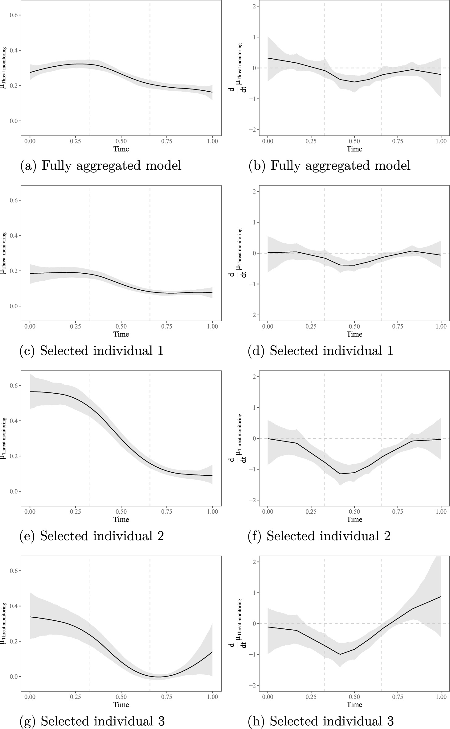
For illustrative purposes, we focus on the derivatives implied by the coefficient functions of the fully aggregated model as well as those implied by the fully person-specific model for three selected individuals with different trajectories. For ease of interpretation, we display the derivatives alongside the corresponding coefficient functions. To convey uncertainty, for both the coefficient functions and their derivatives, we obtained 95% credibility bands by evaluating posterior draws of the coefficient functions on an equally spaced time grid with 200 supporting points and computing the 2.5th and 97.5th percentiles across draws at each grid point.

Figure 5

Coefficient functions (left column) and first-order derivatives (right column) for the mean of nervousness, based on the fully aggregated model and for three selected individuals. Shaded regions represent 95% credibility bands.

Figure 5 Long description

The figure consists of four rows and two columns of line graphs. All graphs share a horizontal X-axis labeled Time, ranging from 0.00 to 1.00. Vertical dashed lines are positioned at approximately 0.33 and 0.66 on the X-axis.

* Left Column (Panels a, c, e, g): The Y-axis is mu sub Nervousness, ranging from 0.0 to 0.6. These panels show coefficient functions.

- Panel a (Fully aggregated model): The curve starts at 0.4, peaks slightly before 0.33, then shows a steady non-linear decline toward 0.2 at Time 1.00.

- Panel c (Selected individual 1): Starts at 0.45, follows a gradual downward slope, leveling off near 0.2 between 0.75 and 1.00.

- Panel e (Selected individual 2): Similar to individual 1 but with a flatter profile, ending at approximately 0.15.

- Panel g (Selected individual 3): Shows a more pronounced dip to 0.15 at Time 0.75 before curving upward toward 0.35 at Time 1.00.

* Right Column (Panels b, d, f, h): The Y-axis is d mu sub Nervousness all over d t, ranging from -2 to 2. These panels show first-order derivatives. A horizontal dashed line marks the zero value.

- Panel b (Fully aggregated model): The derivative peaks sharply above zero at 0.15, drops to a trough near -0.6 at 0.50, and returns toward zero.

- Panel d (Selected individual 1): Shows a shallow peak near zero, a trough at 0.50, and a steady increase toward 0.5 at Time 1.00.

- Panel f (Selected individual 2): Displays a similar oscillating pattern but stays closer to the zero line throughout.

- Panel h (Selected individual 3): Follows the general trough pattern at 0.50 but exhibits a sharp, steep increase reaching above 1.0 at Time 1.00.

In all panels, a solid black line represents the mean, and a light gray shaded region represents the 95% credibility band. The bands generally widen toward the end of the time scale, particularly in the derivative plots for individuals.

Figure 6

Coefficient functions (left column) and first-order derivatives (right column) for the mean of threat monitoring, based on the fully aggregated model and for three selected individuals. Shaded regions represent 95% credibility bands.

Figure 6 Long description

The figure consists of four rows and two columns. All graphs share a horizontal x-axis labeled Time from 0.00 to 1.00. Vertical dashed lines mark time points at approximately 0.33 and 0.66.

Left Column: Coefficient functions for mu sub Threat monitoring. The y-axis ranges from 0.0 to 0.6.

- Row 1 (a) Fully aggregated model: Shows a slight rise to a peak at 0.25 followed by a gradual decline.

- Row 2 (c) Selected individual 1: Displays a lower, flatter curve that begins to decline after 0.33.

- Row 3 (e) Selected individual 2: Starts at a high value of 0.55 and shows a steep, continuous decline until 0.75, where it plateaus.

- Row 4 (g) Selected individual 3: Shows a U-shaped curve that dips to zero at 0.70 before rising sharply at the end.

Right Column: First-order derivatives d over d t of mu sub Threat monitoring. The y-axis ranges from -2 to 2 with a horizontal dashed line at 0.

- Row 1 (b) Fully aggregated model: The curve starts above zero, crosses to negative at 0.25, reaches a trough at 0.50, and returns toward zero.

- Row 2 (d) Selected individual 1: Stays close to zero, dipping slightly negative between 0.33 and 0.75.

- Row 3 (f) Selected individual 2: Shows a deep V-shaped trough reaching -1.2 at time 0.45.

- Row 4 (h) Selected individual 3: Displays a deep trough at 0.45 followed by a sharp linear increase that crosses zero at 0.75 and ends at a positive peak.

In all panels, a solid black line represents the mean, and a light gray shaded region represents the 95 percent credibility bands.

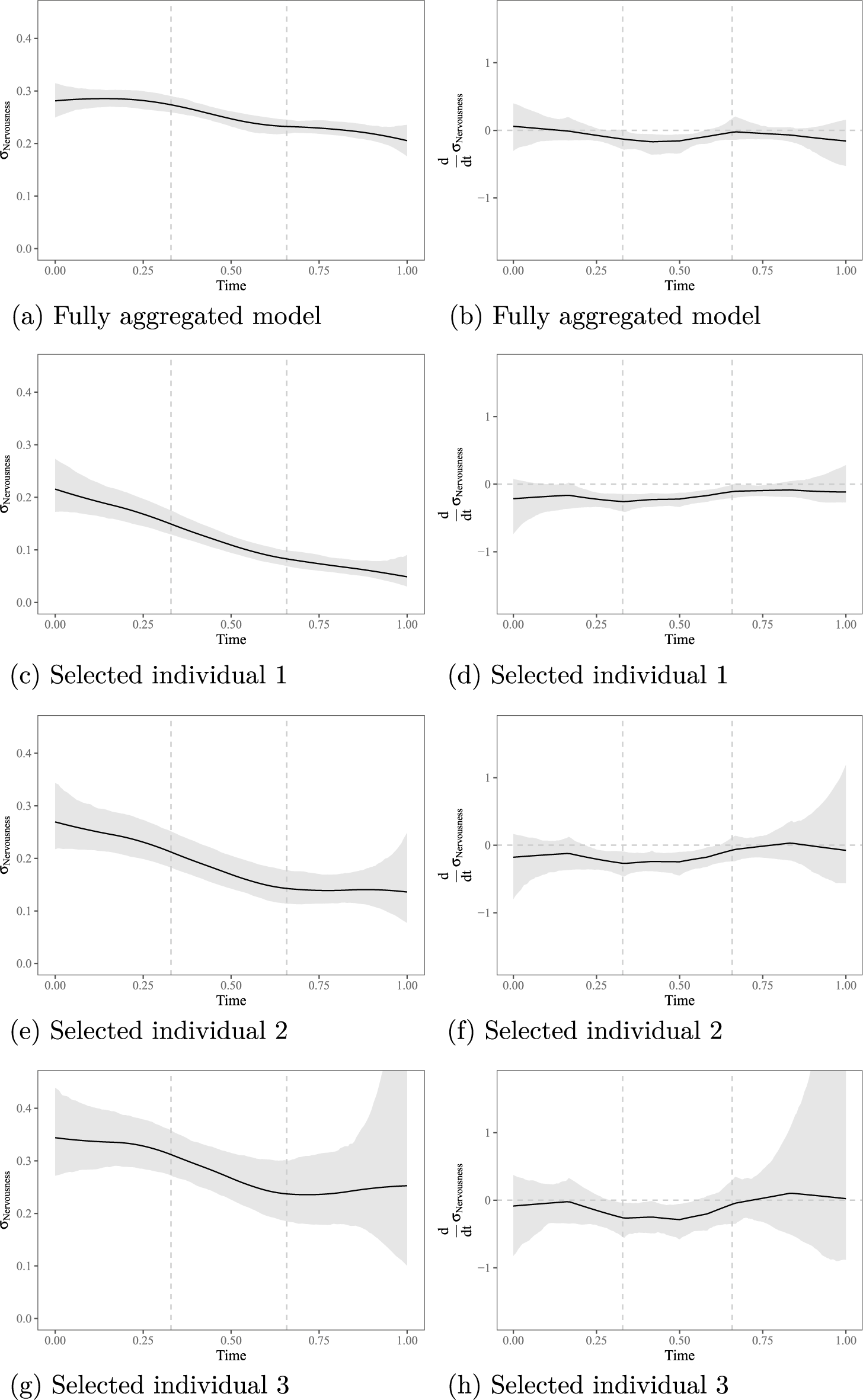
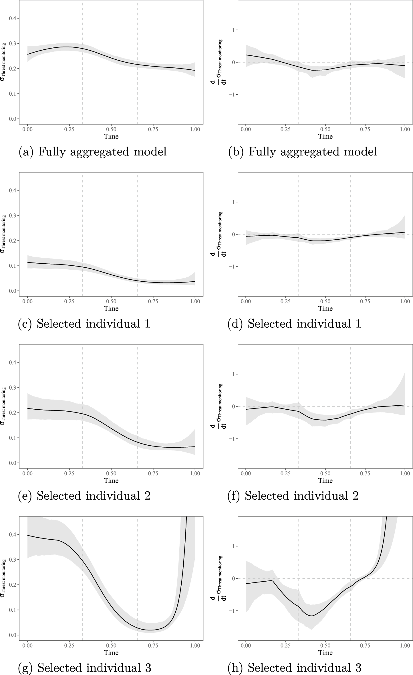
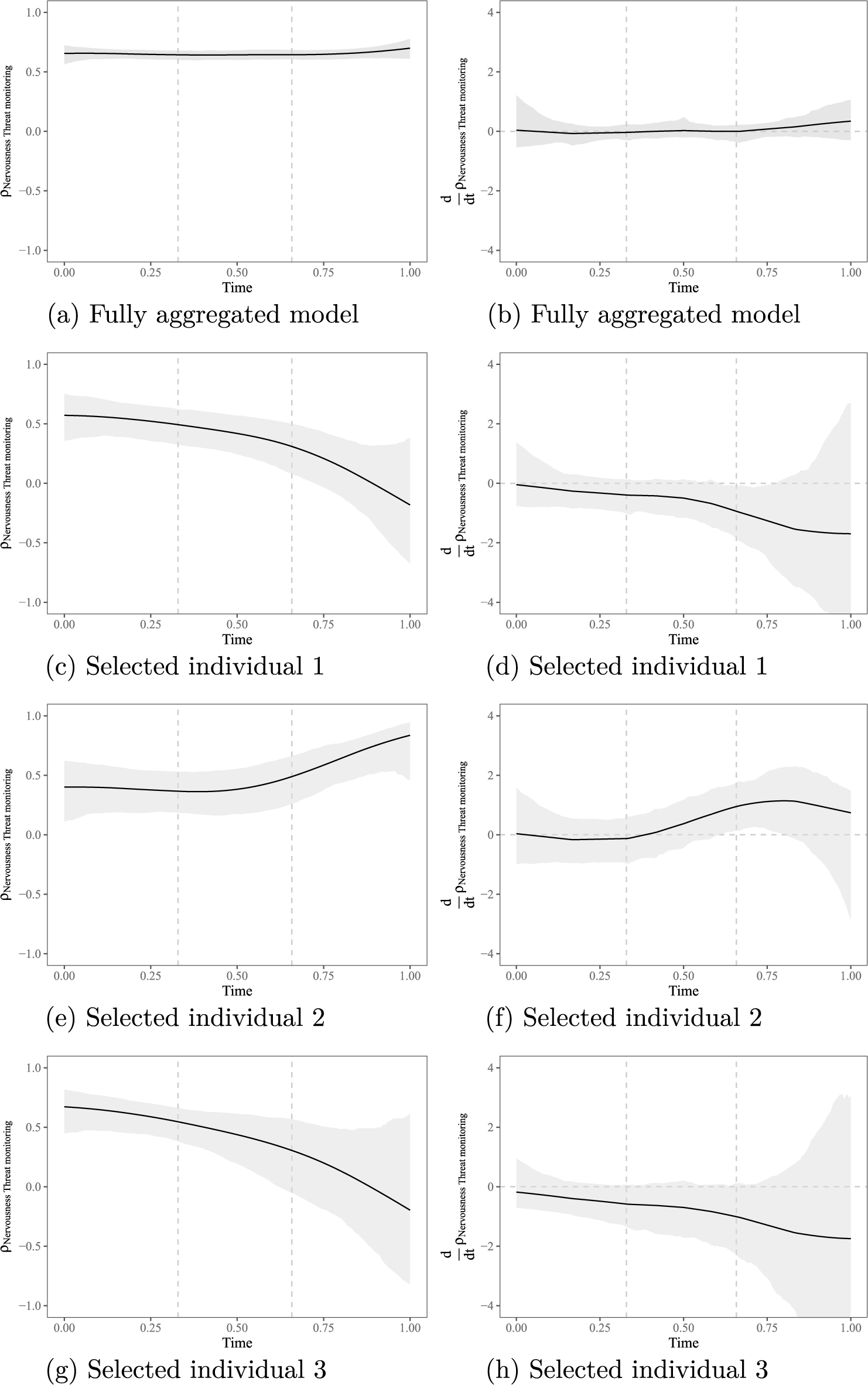
Figures 5 and 6 display derivatives (right columns) alongside the corresponding coefficient functions (left column) for the means of nervousness and threat monitoring, for both the fully aggregated model and selected individuals. In each figure, the black line represents the EAP estimate; the 95% credibility band is depicted in gray. The dashed horizontal line in the right columns marks a change rate of zero, that is, stability. We start by inspecting the time segments before and after therapy for the time-varying mean vectors. For nervousness, a small, positive aggregate-level rate of change credibly different from zero before therapy onset suggests a phase of anticipatory arousal (Figure 5b). For threat monitoring, the aggregate-level rate of change was not credibly different from zero before therapy (Figure 6b). Aggregate-level mean levels of both variables remained stable in the two weeks following therapy. For the three selected individuals, observable deviations from zero rates of change outside of therapy were modest. Therapy, in contrast, marked a period of change at both the aggregate level and for the three selected individuals, with the rate of change being credibly different from zero throughout and peaking approximately one week into therapy.Footnote ⁴ A similar pattern emerged for the standard deviations of nervousness (Figure 7) and threat monitoring (Figure 8). At the aggregate level, the negative rate of change during therapy was more pronounced for the variability of threat monitoring than for nervousness. Note that for individual 3, the rate of change in the standard deviation of nervousness (see Figure 7h) showed only a modest credible deviation from zero during a brief segment of therapy. In contrast, the negative rate of change in the standard deviation of threat monitoring during therapy (see Figure 8h) was most pronounced for this individual, followed by a marked rebound following therapy, with the rate of increase being credibly different from zero. For the correlation of nervousness and threat monitoring (Figure 9), the aggregate trajectory exhibited no rates of change credibly different from zero across the investigated period, and individual trajectories showed only modest credible deviations from zero over brief time segments.

On a general note, the credibility bands in Figures 5–9 indicate that individual-specific coefficient trajectories and their derivatives were estimated with generally high precision, showing only modest reductions in precision relative to the aggregate coefficient functions and their derivatives. This suggests that these estimates can support meaningful conclusions about individual patients’ trajectories, beyond merely describing heterogeneity across individuals. At the same time, precision can vary across coefficients and individuals, as illustrated by the comparison between means and correlations as well as between individual 2, who exhibited only minor losses in precision relative to the fully aggregated model, and individual 3, for whom credibility bands were markedly broader.

7 Possible extensions: Investigating relationships with person characteristics and distal outcomes

After uncovering heterogeneity in patterns of change with hierarchical extensions to TVCM, researchers may be interested in examining whether, and how, such variation relates to person-level characteristics or distal outcomes, such as symptom severity before and after therapy. In the context of therapy research, which is the focus of our running example, understanding heterogeneity in trajectorial patterns as well as their predictive value could contribute to understanding risk factors and mechanisms underlying therapeutic success and support the development of more targeted interventions. Such research objectives can be addressed by modeling individual coefficient function parameters as either outcomes or predictors of person-level characteristics. Here, we discuss how this could be achieved using pre-intervention ( $\text {pre}_i$ ) and three-month follow-up ( $\text {post}_i$ ) anxiety levels as examples. Note that we touch on the integration of person characteristics and distal outcomes only at a theoretical level and do not provide an empirical illustration due to the small sample size of our example data set.

Figure 7

Coefficient functions (left column) and first-order derivatives (right column) for the standard deviation of nervousness, based on the fully aggregated model and for three selected individuals. Shaded regions represent 95% credibility bands.

Figure 7 Long description

The figure consists of eight panels labeled a through h. All graphs share a common x-axis labeled Time, ranging from 0.00 to 1.00, with vertical dashed lines at approximately 0.33 and 0.66.

Left Column (Panels a, c, e, g): The y-axis is sigma sub Nervousness, ranging from 0.0 to 0.4.

- Panel a (Fully aggregated model): Shows a gradual, slightly concave decrease from 0.28 to 0.20.

- Panel c (Selected individual 1): Shows a steeper, nearly linear decline from 0.22 to 0.05.

- Panel e (Selected individual 2): Shows a curve starting at 0.27, decreasing to a plateau of 0.14 after time 0.75.

- Panel g (Selected individual 3): Shows a curve starting at 0.34, dipping to 0.24, and slightly rising at the end.

Right Column (Panels b, d, f, h): The y-axis is d sigma sub Nervousness over d t, ranging from -1 to 1, with a horizontal dashed line at 0.

- Panel b (Fully aggregated model): The derivative fluctuates slightly below zero, indicating the slow rate of decline.

- Panel d (Selected individual 1): The derivative is consistently negative, reflecting the steady decline in panel c.

- Panel f (Selected individual 2): Shows a wave-like derivative that approaches zero toward the end.

- Panel h (Selected individual 3): Shows a derivative that dips below zero and returns to zero, with significantly widening shaded credibility bands after time 0.75.

In all panels, a solid black line represents the mean estimate, and a light gray shaded region represents the 95% credibility band. The uncertainty bands are generally narrowest in the aggregated model and widest for individual 3.

Figure 8

Coefficient functions (left column) and first-order derivatives (right column) for the standard deviation of threat monitoring, based on the fully aggregated model and for three selected individuals. Shaded regions represent 95% credibility bands.

Figure 8 Long description

The figure consists of eight panels labeled a through h. All graphs share a common x-axis for Time ranging from 0.00 to 1.00. Vertical dashed lines mark time points at approximately 0.33 and 0.66.

* Row 1 (Fully aggregated model): Panel a shows sigma Threat monitoring on the y-axis (0.0 to 0.4). The curve starts at 0.25, peaks slightly before 0.25 time, then gradually declines to 0.2. Panel b shows the derivative d over d t of sigma Threat monitoring on the y-axis (-1 to 1). The curve fluctuates near zero, dipping slightly below between the dashed lines.

* Row 2 (Selected individual 1): Panel c shows a lower sigma starting at 0.1, decreasing slowly to near 0.05. Panel d shows a nearly flat derivative curve hovering just below the zero line.

* Row 3 (Selected individual 2): Panel e shows sigma starting at 0.2, maintaining a plateau until the first dashed line, then dropping sharply to 0.05. Panel f shows the derivative dipping to -0.5 between the dashed lines before returning to zero.

* Row 4 (Selected individual 3): Panel g shows high variability, with sigma starting at 0.4, plunging to near 0.0 at time 0.75, and then spiking vertically toward 0.5. Panel h shows the derivative dropping sharply to -1.0 at time 0.4 and then rising steeply to above 1.0 after time 0.75.

In all panels, a solid black line represents the mean, and a light gray shaded region represents the 95% credibility band.

Figure 9

Coefficient functions (left column) and first-order derivatives (right column) for the correlation of nervousness and threat monitoring, based on the fully aggregated model and for three selected individuals. Shaded regions represent 95% credibility bands.

Figure 9 Long description

The multi-panel display consists of four rows and two columns. All panels share a horizontal x-axis labeled Time, ranging from 0.00 to 1.00. The left column y-axis is rho sub Nervousness Threat monitoring, ranging from -1.0 to 1.0. The right column y-axis is d over d t rho sub Nervousness Threat monitoring, ranging from -4 to 4.

* Row 1 (a and b): Fully aggregated model. Panel a shows a nearly horizontal line at y equals 0.6. Panel b shows a flat derivative line at y equals 0.

* Row 2 (c and d): Selected individual 1. Panel c shows a downward curve starting at 0.6 and ending near -0.2. Panel d shows a corresponding negative derivative that dips further below zero as time increases.

* Row 3 (e and f): Selected individual 2. Panel e shows a U-shaped curve that begins at 0.4, dips slightly, and rises to 0.8. Panel f shows the derivative crossing from negative to positive, peaking around time 0.75.

* Row 4 (g and h): Selected individual 3. Panel g shows a steady decline from 0.7 to -0.2. Panel h shows a consistent negative derivative.

In all panels, a solid black line represents the mean, and light gray shaded regions indicate 95% credibility bands. Vertical dashed lines are positioned at time 0.33 and 0.66 across all graphs.

7.1 Coefficients as outcomes

When the aim is to explain heterogeneity in coefficient functions, between-person characteristics can be included as predictors of the coefficient functions’ person-specific parameters. For example, if researchers want to explain heterogeneity in the trajectory of a symptom’s severity using pre-intervention anxiety levels, coefficients describing individual-specific time-varying means could be modeled as follows:

(14) $$ \begin{align} a_{i,x0}& \sim \mathcal{N}(\beta_{0,ax0}+\beta_{1,ax0}\cdot\text{pre}_i,\phi_{ax0})\\ a_{i,x1}& \sim \mathcal{N}(\beta_{0,ax1}+\beta_{1,ax1}\cdot\text{pre}_i,\phi_{ax1}) \notag\\ a_{i,x2}& \sim \mathcal{N}(\beta_{0,ax2}+\beta_{1,ax2}\cdot\text{pre}_i,\phi_{ax2}) \notag \\ a_{i,x,2+k} &\sim \mathcal{N}(\beta_{0,ax,2+k}+\beta_{1,ax,2+k}\cdot\text{pre}_i,\omega_{ax,k}) \quad \text{for } k = 1, 2, \ldots, K. \notag \end{align} $$

To examine the results, researchers can plot model-implied coefficient functions for individuals with varying values on the considered covariate(s), or assess the extent to which unexplained variability in the parameters defining the coefficient functions (i.e., $\phi _{ax0}$ , $\phi _{ax1}$ , $\phi _{ax2}$ , and $\omega _{ax,k}$ ) is reduced upon inclusion of a given covariate.Footnote ⁵

7.2 Coefficients as predictors

When the aim is to investigate whether person-specific trajectories help explain distal outcomes—such as three-month follow-up anxiety levels while controlling for pre-intervention anxiety—the person-specific parameters of the coefficient functions can be used as predictors (see Gloster et al., Reference Gloster, Nadler, Block, Haller, Rubel, Benoy, Villanueva, Bader, Walter, Lang, Hofmann, Ciarrochi and Hayes2024; McCormick & Bauer, Reference McCormick and Bauer2024; Neubauer et al., Reference Neubauer, Brose and Schmiedek2023, for examples using coefficients from linear models). Suppose a researcher is interested in examining whether initial levels of coupling between nervousness and threat monitoring predict post-therapy anxiety levels. They could do so by modeling the individual-specific correlation coefficient intercepts as predictors, controlling for pre-intervention anxiety:

(15) $$ \begin{align} \text{post}_i \sim \mathcal{N}(\gamma_0 + \gamma_p\cdot\text{pre}_i+\gamma_{c}\cdot c_{i0},\xi). \end{align} $$

If the researcher is interested in whether trajectories of this coupling across therapy explain differences in post-therapy anxiety levels, all individual-specific coefficients describing these trajectories alongside their interactions could be included in the model. As the number of regression coefficients can become high quite quickly—for example, for large K or when trajectories of multiple parameters are considered—we strongly recommend regularizing the regression coefficients $\gamma $ to stabilize estimation (see, e.g., Kaplan, Reference Kaplan2023; van Erp, Reference van Erp, Schoot and Miočević2020, for introductions). We note that the regression coefficients ( $\gamma $ ) may be difficult to interpret. To address this, researchers can instead examine reductions in unexplained variability ( $\xi $ ) from the block-wise inclusion of parameters.