


Impact statement
This study presents an interpretable machine learning framework for predicting crack evolution in beam bridges. By identifying key deterioration factors and providing accurate forecasts (R2 > 0.94), the research bridges the gap between prediction accuracy and model transparency. The findings enable targeted maintenance strategies by demonstrating that traffic loading and aging contribute over 60% to crack development, advancing both theoretical understanding and practical infrastructure management approaches.
1. Introduction
Bridges constitute critical components of transportation infrastructure, carrying substantial daily traffic volumes and playing a pivotal role in societal and economic development (Ebrahimpour et al., Reference Ebrahimpour, Baibordy and Ibrahim2025; Zhang et al., Reference Zhang, Ren, He, Gao, Li and Song2025). As bridges age, they face multiple challenges, including structural deterioration, environmental corrosion, and increasing traffic loads. Consequently, accurate bridge condition assessment has become increasingly crucial for ensuring operational safety. Current assessment methodologies primarily rely on periodic inspections, non-destructive testing, monitoring systems, and deterioration studies. Contemporary research endeavors focus on comprehensively understanding bridge deterioration processes, identifying root causes, and developing targeted maintenance strategies.
From the perspective of research paradigms, existing studies on bridge condition assessment and deterioration forecasting can broadly be categorized into three developmental pathways: (1) experience- and inspection-based condition rating methods, (2) mechanistic modeling approaches grounded in structural reliability theory, and (3) data-driven machine learning methods. Conventional manual visual inspection and non-destructive testing have established the foundation for bridge condition assessment, and have enabled quantitative descriptions of bridge technical condition through composite indices (Xin et al., Reference Xin, Jiang, Wu and Yang2023). Building on this, structural reliability approaches further introduce probability theory and stochastic processes to characterize the evolution of bridge deterioration. Brighenti et al. (Reference Brighenti, Bado, Romeo and Zonta2024) combined Markov chains with defect evolution models to develop a bridge decision-support system capable of forecasting future reliability and failure risk.
However, prior research has shown that reliability- and physics-based models often underutilize long-term accumulated inspection data in practical engineering applications. For instance, although Dena et al. (Reference Dena, Behrouz and Basak2023) incorporated physical models within a data-assisted deterioration forecasting framework to improve predictive accuracy, their approach still relies primarily on predefined deterioration assumptions and therefore struggles to fully capture the statistical characteristics and nonlinear relationships embedded in multi-source inspection data. In addition, such models are typically computationally intensive and require costly parameter calibration, which constrains their scalability and wider deployment across large bridge networks.
With the continuous growth in the volume and diversity of bridge inspection and monitoring data, research has increasingly shifted toward data-driven approaches. Machine learning models can automatically extract latent patterns from large-scale historical inspection records and have, therefore, been widely adopted for predicting bridge condition ratings and load-carrying capacity (Qian et al., Reference Qian, Hongfan, Baidurya, Tawil, Agrawal and Wong2024). For example, Xia et al. (Reference Xia, Lei, Wang and Sun2021) integrated regional bridge inspection reports with monitoring information to enable network-level condition assessment. Zhang et al. (Reference Zhang, Lei, Xia and Sun2024) employed large language models to support the construction of bridge databases, improving data quality and modeling efficiency. Alipour et al. (Reference Alipour, Harris, Barnes, Ozbulut and Carroll2022) further demonstrated the effectiveness of models such as random forests (RF) for bridge load capacity prediction.
While data-driven models have shown strong performance in predicting network-level condition ratings and load capacity, their reliability ultimately depends on the availability of accurate, fine-grained defect information at the component level, motivating increasing attention to defect detection as a fundamental step in bridge health assessment.
In the context of bridge defect research, cracks—being the most common and representative form of structural damage—have attracted substantial attention in recent years. To date, extensive progress has been made worldwide in bridge crack detection and recognition, with research efforts primarily focusing on automated crack detection, localization, and geometric feature extraction. For example, Ni et al. (Reference Ni, Mao, Fu, Wang, Zong and Luo2023)proposed a deep-learning-based approach for the automatic detection and localization of deck cracks and other pavement-related defects. Their method employs YOLOv7 to achieve high-accuracy identification of multiple defect types and integrates an improved LaneNet network to perform lane-level spatial localization of cracks. Validation on multi-source in situ bridge-deck datasets showed that the framework maintains strong robustness and real-time performance under complex illumination conditions and traffic-related interference, demonstrating the applicability of deep learning to practical automated crack inspection. Dong et al. (Reference Dong, Yuan and Dai2025) similarly applied deep learning to enable automatic crack detection and localization, achieving favourable performance in terms of detection accuracy and robustness, and highlighting the potential of data-driven approaches for crack recognition. Cui et al. (Reference Cui, Yan, Feng, Wu and Zhu2025) combined YOLOX with ultra-wideband (UWB) positioning to develop a UAV-based crack detection and spatial localization method, enabling real-time crack identification and three-dimensional localization in GNSS-constrained environments such as beneath bridges. Wu et al. (Reference Wu, Shi, Ma and Liu2024) further enhanced the YOLOv5 model by introducing a convolutional block attention module (CBAM), significantly improving crack detection accuracy across multiple crack image datasets. Collectively, these studies indicate that deep-learning-based crack detection has achieved substantial advances in both recognition accuracy and automation.
However, in terms of research objectives and practical deployment, existing crack-related studies largely remain at the stage of static detection—that is, identifying crack morphology and quantifying geometric attributes—while paying comparatively limited attention to the dynamic evolution of cracks over time. Most approaches focus on recognizing and measuring crack states at a single inspection epoch and have yet to effectively characterize long-term crack propagation patterns and associated risks during service. This limitation, to some extent, constrains the engineering value of crack information in bridge deterioration forecasting and maintenance decision-making.
Moreover, current crack detection research typically relies on image data as the sole information source, and thus does not fully exploit the long-term accumulated historical crack records embedded in periodic inspection reports, nor their intrinsic relationships with structural characteristics and traffic loading. As a result, existing studies face challenges in providing deeper insight—at the level of crack development—into the dominant drivers and underlying mechanisms governing the degradation of bridge structural performance.
Overall, the literature suggests that while data-driven approaches show considerable promise for bridge condition forecasting, existing studies still predominantly formulate prediction tasks around composite condition indices derived from periodic inspections. As highlighted by Xia et al. (Reference Xia, Lei, Wang and Sun2021) and Liang et al. (Reference Liang, Zhang, Huang, Hu and Zhang2025), inspection reports remain the primary data source for large-scale condition assessment, but their information is typically organized as management-oriented condition descriptions that require extensive extraction and standardization before being converted into machine-readable variables for modeling. This paradigm leads to several limitations. (1) Because outputs are often expressed as overall scores or rating levels, it becomes difficult to directly characterize the evolution of specific defects, such as cracking, at a defect-parameter level. (2) Although inspection reports contain considerable defect-related and condition-related information, including quantitative descriptors, such information has not yet been systematically exploited for deterioration modeling in a standardized and reusable form, largely due to heterogeneity, missing entries, and human-induced uncertainty in the reporting process. (3) In addition, the direct cumulative effects of traffic loading on defect evolution are rarely modelled explicitly: Xia et al. emphasize that traffic indicators (e.g., ADT and ADTT) must be extracted and incorporated to reflect service load variation and regional performance correlation, implying that omitting these variables may overlook a key deterioration driver. (4) Finally, even when predictive performance is improved, model outputs often lack engineering transparency; therefore, additional analysis—such as correlation exploration and factor attribution—remains necessary to extract deterioration characteristics and to support maintenance decision-making at the network level.
In terms of methodological choices, conventional neural network models exhibit strong nonlinear approximation capability, but they typically require large sample sizes and often lack interpretability. In contrast, ensemble learning methods tend to provide better generalization while maintaining competitive predictive accuracy (Nasrin et al., Reference Nasrin, Bateni, Changhyun, Heggy and Band2023; Wang et al., Reference Wang, Philippe, Christophe, Zhu, Chen and Schmidt2023; Fard and Fard, Reference Fard and Fard2024). Among these, XGBoost incorporates regularization and a gradient boosting scheme, achieving high stability and predictive performance in complex nonlinear problems (Hou and Zhou, Reference Hou and Zhou2020; Li et al., Reference Li, Zhou, Shen and Zhao2024; Sheng et al., Reference Sheng, Ren, Wang, Li and Li2024; Qi et al., Reference Qi, Lin, Yang and Liang2025). When combined with interpretability techniques such as SHAP, the contributions of individual input variables to crack development can be quantified, thereby addressing the limited interpretability of traditional machine learning models.
Based on the above analysis, this study investigates more than 100 hollow-slab girder bridges along an expressway corridor. Instead of relying solely on crack detection outcomes, crack density (CD) and maximum crack width (MCW) are adopted as quantitative indicators to characterize crack evolution. A multi-source bridge condition database is constructed, an XGBoost model is developed to predict crack development, and SHAP is introduced to interpret key influencing factors. The proposed framework aims to improve predictive accuracy while systematically elucidating the mechanisms through which traffic loading, bridge age (BA), and other factors affect crack evolution, thereby providing more reliable data support and theoretical evidence for bridge maintenance decision-making.
The remainder of this paper is structured as follows: Section 2 introduces the technical framework for predicting beam crack parameters in small- and medium- span hollow slab bridges. Section 3 details the methods and processes for establishing the bridge state database through the integration and standardization of multi-source information. Section 4 describes the construction of the bridge degradation models based on machine learning algorithms, including correlation analysis of parameters, model training and tuning, and comparative analysis of prediction performance across different models. Section 5 presents the interpretability analysis of the XGBoost model using the SHAP algorithm to identify key factors influencing main beam crack development. Finally, Section 6 summarizes the findings and conclusions of this study.
2. Technical framework
This paper proposes a technical framework for predicting main beam crack parameters in small- and medium-span hollow slab bridges, as illustrated in Figure 1. The framework comprises the following key components:
-
1) Database construction: During the mining and integration of multi-source information, data wrangling techniques are employed to establish a bridge condition database.
-
2) Model training and testing: Degradation features are extracted from the constructed raw database, followed by data preprocessing and wrangling, yielding a bridge condition dataset. Considering the direct impact of vehicular loads on crack development and the cumulative effect of traffic volume over time, the SVR, RF, and XGBoost models are trained using the bridge dataset to derive an optimal crack parameter prediction model. This model is evaluated, validated, and subsequently enables the prediction of crack development trends in individual bridge beams.
-
3) Interpretability analysis: the SHAP algorithm is applied to perform interpretability analysis on the XGBoost model, yielding a ranking of feature importance and thereby identifying key factors influencing main beam crack development. These findings provide a reliable basis for formulating subsequent bridge management and maintenance decisions.
Technical roadmap.

3. Integration and standardization of multi-source information
This section mainly introduces the methods and processes for establishing the bridge state database, as shown in Figure 2.
Bridge condition database flowchart.

3.1 Data source
Hollow slab bridges constitute a widely adopted bridge type within China’s expressway network. Their hollow chamber structure is highly susceptible to cracking during long-term service. Once these cracks propagate, they not only diminish the stiffness and load-bearing capacity of bridge beams but may also induce structural failure, posing a significant threat to traffic safety. Small- and medium-span bridges account for over 80% of the total in-service bridge inventory in China, representing the predominant structural form within the transportation network. Consequently, their operational status critically influences overall transportation safety.
Based on this context, this research focuses on predicting crack development in small- and medium-span hollow slab bridges located along a specific expressway. The superstructures of the selected bridges are all precast hollow slab systems, with construction years ranging from 2002 to 2010. Through extensive and periodic bridge inspections, structural deterioration information during the operational phase of bridges within the region can be acquired. Within the bridge management system, in accordance with the Technical Condition Evaluation Standard for Highway Bridges, inspection information comprises two categories: (1) Bridge defects and their scales directly obtained through inspection; (2) Technical condition scores for the entire bridge or its components, calculated using a hierarchical weighting method. Bridge management authorities record and store this inspection data as mandated by regulations.
This study leverages extensive inspection data accumulated over years of operation and maintenance from over 100 small- and medium-span hollow slab bridges along an expressway. Incorporating variations in extreme high/low temperatures (EHT/ELT), environmental humidity (EH), and air pollutant concentrations(APC) within the region (where air pollutant concentration is characterized by the air quality index (AQI) of the bridge location), while also accounting for the direct influence of vehicle load (VL) on bridge performance degradation, and combined with information on individual bridge attributes and main beam crack parameters, a bridge condition database is established.
Beyond bridge inspection reports, supplementary data sources include bridge monitoring information and construction drawings. Among these, bridge inspection reports (technical condition assessment forms), preserved in easily stored electronic formats, remain highly complete and provide the most comprehensive documentation of main beam crack information. The technical condition assessment forms record critical structural attributes (e.g., configuration characteristics, service life, damage conditions, and assessment scores), encompassing the majority of features characterizing main beam crack parameters in bridges. Given that compiling the massive historical data from multi-year technical condition assessment forms is challenging, big data automation techniques are employed to efficiently acquire the required key input data and facilitate the construction of the database. Furthermore, since the transportation network serves the core functions of passage and freight during the service life, VL constitutes one of the most significant external influences. Consequently, traffic volume data significantly impacts the assessment of main beam crack parameters for individual bridges. However, traffic volumes and VL information cannot be obtained directly from bridge inspection reports. Therefore, monitoring data, including historical annual average daily traffic (ADT), annual average daily truck traffic (ADTT) statistics, and time-accumulated VL for individual bridges, is acquired via bridge weigh-in-motion systems, supplementing the bridge condition database. The database constructed in this study comprises a total of 400 samples derived from 100 bridges.
An in-depth analysis of crack information within bridge inspection reports was conducted, employing statistical analysis methods to mine and analyze the main beam crack data. Following the preprocessing of the crack data, multidimensional and hierarchical statistical analysis was performed. This led to the selection of MCW and CD of the main beam as the parameters characterizing crack development. It is noted that CD is defined as the average main beam crack length divided by bridge length (average crack length/bridge length), with the average crack length derived by dividing the total length of main beam cracks by the number of cracks.
3.2 Data integration and preprocessing
This section establishes a set of bridge data integration rules tailored for crack development prediction, with the bridge serving as the core entity. Multi-source heterogeneous data are systematically organized using a unified “category- attribute-attribute value” structure. Specifically, the bridge category is defined as the top-level entity, within which both static and dynamic attributes—such as bridge length and BA—are specified to characterize the geometric properties and service conditions of each bridge. On this basis, a crack category is introduced as a key damage subclass to consistently describe crack-related indicators, including total crack length and MCW, thereby enabling explicit association between crack information and bridge entities. In addition, a traffic category is incorporated as an operational environmental factor of the bridge, with attributes such as ADT used to represent traffic flow effects. At the instance level, all attributes are assigned using standardized units and clearly defined semantics, allowing for the integrated representation of bridge basic information, damage characteristics, and external influencing factors. This integration rule framework provides a well-structured and semantically consistent data foundation for subsequent crack feature extraction, temporal analysis, and predictive model development. Figure 3 summarizes the proposed data integration rules.
Schematic diagram of data integration rules and structure.

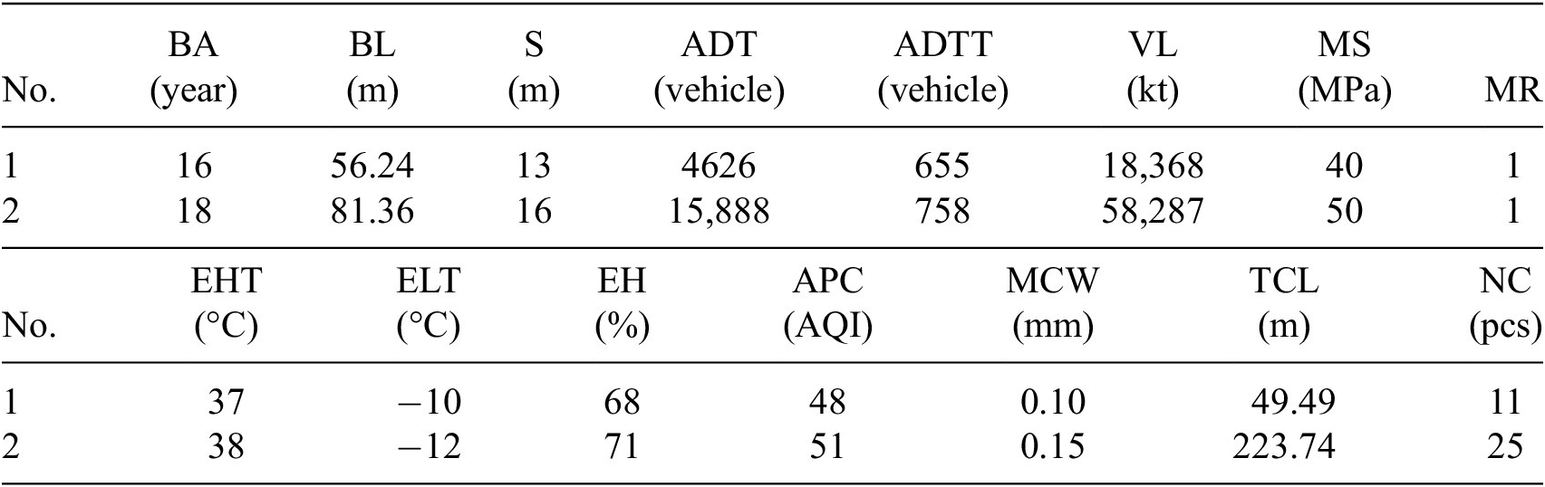
Acquiring the corresponding data objects for an individual bridge involves the following steps: (1) Identifying and extracting semi-structured or unstructured data obtained in textual form; (2) Retrieving feature attributes and their corresponding values from the bridge inspection reports. The acquired data objects must encompass the following information: (1) Basic structural information of the individual bridge; (2) Feature parameter information influencing crack development; (3) Fundamental information regarding main beam cracks. A comprehensive bridge condition database must encompass generated data units for each bridge. This is implemented as follows: A record table is generated, where each row represents the state information of an individual bridge for a specific year, and each column represents a different attribute value characterizing the bridge’s state. The database encompasses the basic structural information, key feature parameters, main beam crack information, as well as the traffic flow and VL monitoring information for the respective year of the specified bridges. An illustrative example is provided in Table 1. In Table 1, the meanings of other abbreviations are defined as BA representing the bridge age, BL representing the bridge length, S representing the bridge span, MR representing the maintenance record, MS representing the material strength, TLC representing the total length of cracks, and NC representing the number of cracks.
Example of the bridge condition database

Owing to suboptimal data integrity in paper records, inconsistent formats and standards of electronic inspection reports, and human-induced data omissions, the quality of data across different sources within the raw database exhibits significant heterogeneity. Consequently, these data cannot be directly utilized for subsequent analytical procedures. Thus, the integrated raw database necessitates cleansing to identify and address outliers, thereby enhancing the accuracy of subsequent algorithms.
Data cleansing constitutes the core step of the preprocessing phase, primarily addressing issues such as missing values, outliers, and duplicate records. For missing data, imputation methods (e.g., mean imputation, median imputation, or interpolation) may be employed, or deletion may be selected if the proportion of missing values is high and their impact on the model is negligible. Following the identification of outliers using statistical methods (e.g., box plots or Z-scores), a decision is made to either remove or correct them based on the specific context. Completely duplicate data records are directly removed.
Specifically, the raw inspection records were first screened to remove samples with missing critical information, including the inspection year, crack measurement parameters (such as crack width or crack length), and key traffic indicators. These variables are regarded as essential for characterizing the structural condition of a bridge at a specific year, and their absence would prevent a sample from accurately representing the actual service state. Therefore, samples lacking such critical information were directly excluded from subsequent analysis.
For non-critical feature variables with occasional missing values (e.g., certain environmental factors), missing entries were imputed using historical averages from the same bridge whenever available. This decision is based on the consideration that environmental influences on crack development are typically indirect and cumulative, and short-term fluctuations are less influential than long-term trends. By using bridge-specific historical averages, this strategy avoids introducing information from other bridges while preserving the temporal continuity and internal consistency of each individual bridge, thereby providing a reliable data basis for crack evolution modeling.
With respect to outlier treatment, this study does not rely solely on mechanical statistical thresholds but instead adopts a combined approach integrating statistical inspection and engineering judgment. Initially, potential outliers are identified by examining the distribution characteristics of crack parameters and related feature variables, focusing on samples that exhibit values significantly deviating from typical ranges. Subsequently, these samples are further examined in conjunction with the corresponding maintenance and repair records of the bridges. Samples exhibiting abnormal crack parameter jumps without any associated maintenance, strengthening, or exceptional event records are considered likely to result from measurement errors, recording inaccuracies, or data processing artifacts, and are, therefore, removed from the dataset.
By incorporating engineering context into the outlier identification process, the proposed preprocessing strategy avoids misinterpreting non-physical abnormal records as genuine deterioration behavior, thereby reducing their adverse impact on model training and improving the stability and reliability of the prediction results.
Through the aforementioned steps, the cleansing of bridge inspection and monitoring data is completed. A comprehensive flowchart of the bridge condition database is illustrated in Figure 2.
3.3 Problem-oriented data regularization
A subset of feature attributes is selected from the raw database. BA, BL, S, MR, MS, ADT, ADTT, and VL are defined as the parameter set most relevant to main beam crack development. Redundant attributes are subsequently removed.
Based on computer-extractable data types, the data formats within attribute subsets are transformed. BA is a directly representable numerical attribute and requires no transformation. The transformation method for ADT aligns with that of BA. MR is a boolean-type input encoded as {0, 1}. A value of 1 indicates maintenance performed in the inspection year, while 0 denotes no maintenance. Input and output attributes (excluding MR) are subsets of the original attribute set. Thus, their data types match the original attributes but require further encoding into machine learning-compatible formats, as specified in Table 2. For numerical attributes, significant value-range disparities across features may skew the importance weighting of attributes during model computation. For instance, S typically ranges between 10 and 40 m, whereas VL may range from 1.7 × 10⁷ to 5 × 10⁸ t. The orders of magnitude between S and VL differ drastically; thus, VL may disproportionately diminish the influence of S during modeling. Furthermore, dimensional heterogeneity across features introduces incomparability. To enhance model generalizability, this study employs standardized preprocessing. Log-transformation normalizes data into a compact scale, diminishing the dominance of large values while amplifying distinctions among smaller values.
 $$ {x}^{\prime }=\frac{\log \left(x+1\right)}{\log \left({x}_{max}+1\right)} $$
where $ x $
denotes the raw data value,
$ x $
denotes the raw data value, $ {x}_{max} $
represents the maximum raw data value, and
$ {x}_{max} $
represents the maximum raw data value, and $ {x}^{\prime } $
is the normalized result confined to the [0,1] interval. The normalization procedure is primarily applied to numerical attributes. Specifically, MR within input features adopts binary values {0,1}, indicating whether the main beams underwent maintenance in the recorded year, thus requiring no additional encoding. For the output parameters proposed in this study, that is, MCW and CD, their values are naturally constrained within the [0,1] interval, thereby eliminating the need for further encoding transformations.
$ {x}^{\prime } $
is the normalized result confined to the [0,1] interval. The normalization procedure is primarily applied to numerical attributes. Specifically, MR within input features adopts binary values {0,1}, indicating whether the main beams underwent maintenance in the recorded year, thus requiring no additional encoding. For the output parameters proposed in this study, that is, MCW and CD, their values are naturally constrained within the [0,1] interval, thereby eliminating the need for further encoding transformations.
Input and output parameters of the model

4. Bridge degradation modeling based on machine learning
4.1. Machine learning algorithm
This study mainly adopts the XGBoost algorithm. XGBoost is an efficient ensemble learning method that fundamentally employs decision trees and enhances predictive performance through optimized objective functions (Kumar et al., Reference Kumar, Arora and Nehdi2024). Compared to traditional gradient boosting trees, XGBoost incorporates optimizations, including regularization control, node-splitting sorting, and automated missing-value handling. These enhancements accelerate training while improving prediction accuracy. Similar to RF, XGBoost regression generates final predictions as weighted averages of outputs from multiple decision trees. During tree construction, it autonomously evaluates feature importance/weights and selects optimal features/nodes for splitting, enabling efficient regression. The XGBoost objective function extends beyond loss terms. It introduces regularization terms (Chen et al., Reference Chen, He and Kong2025) to control model complexity and mitigate overfitting, that is,
 $$ \varOmega (f)=\gamma T+\frac{1}{2}\lambda \parallel w{\parallel}^2 $$
where $ \gamma $
and
$ \gamma $
and $ \lambda $
represent penalty coefficients,
$ \lambda $
represent penalty coefficients, $ T $
denotes the number of leaf nodes, while
$ T $
denotes the number of leaf nodes, while $ w $
signifies the predictive weight assigned to each leaf node within the tree.
$ w $
signifies the predictive weight assigned to each leaf node within the tree.
XGBoost employs incremental training (Chen et al., Reference Chen, Zhang, Li and Zhou2025) to maximize loss function reduction during optimization. After round t iteration, the objective function can be expressed as
 $$ Obj\left(\theta \right)=\sum \limits_{i=1}^nl\left({y}_i,{\hat{y}}_i^{\left(t-1\right)}+{f}_t\left({x}_i\right)\right)+\varOmega \left({f}_t\right)+ Const $$
where $ l $
denotes the loss function, while
$ l $
denotes the loss function, while $ {y}_i $
represents the true value,
$ {y}_i $
represents the true value, $ {\hat{y}}_i^{\left(t-1\right)} $
is the predicted value after the
$ {\hat{y}}_i^{\left(t-1\right)} $
is the predicted value after the $ \left(t-1\right) $
th iteration, and
$ \left(t-1\right) $
th iteration, and $ {f}_t\left({x}_i\right) $
corresponds to the prediction function of the
$ {f}_t\left({x}_i\right) $
corresponds to the prediction function of the $ t $
th tree. The term Const denotes constant terms independent of optimization.
$ t $
th tree. The term Const denotes constant terms independent of optimization.
In addition, two commonly used machine learning algorithms, that is, SVR and RF, are also used in this study to compare the performance between different algorithms. The aforementioned machine learning models are employed to characterize crack degradation in voided slab beam bridges. Input parameters include: BA, BL, S, ADT, ADTT, VL, MS, EHT, ELT, MR, EH, and APC. Predictive targets comprise MCW and CD, which quantitatively characterize crack propagation, as detailed in Table 2.
4.2. Parameter correlation analysis
Significant multicollinearity in machine learning algorithms may compromise output stability (Alsaif and Abbas, Reference Alsaif and Abbas2024). Thus, correlation analysis among input parameters is essential when processing crack prediction datasets from over 100 voided hollow slab bridges, ensuring analytical accuracy and reliability. Heatmaps intuitively visualize data distributions and variable correlations through color intensity gradients, where darker hues indicate stronger correlations. These graphical representations display correlation coefficient matrices for parameters. The correlation coefficient can be calculated as:
 $$ {\rho}_{x_1,{x}_2}=\frac{Cov\left({X}_{1,}{X}_2\right)}{\sqrt{D{X}_1,D{X}_2}}=\frac{E{X}_1{X}_2-E{X}_1\ast {X}_2}{\sqrt{D{X}_1\ast D{X}_2}} $$
where $ Cov $
denotes the covariance between parameters
$ Cov $
denotes the covariance between parameters $ {X}_1 $
and
$ {X}_1 $
and $ {X}_2 $
;
$ {X}_2 $
; $ E $
represents the mathematical expectation;
$ E $
represents the mathematical expectation; $ D $
signifies the variance;
$ D $
signifies the variance; $ \rho $
is the correlation coefficient between parameters
$ \rho $
is the correlation coefficient between parameters $ {X}_1 $
and
$ {X}_1 $
and $ {X}_2 $
, with its value ranging from −1 to 1 inclusive. The closer the absolute value of
$ {X}_2 $
, with its value ranging from −1 to 1 inclusive. The closer the absolute value of $ \rho $
is to 1, the stronger the positive or negative linear correlation between parameters
$ \rho $
is to 1, the stronger the positive or negative linear correlation between parameters $ {X}_1 $
and
$ {X}_1 $
and $ {X}_2 $
. A correlation coefficient of 0 indicates no linear relationship between parameters
$ {X}_2 $
. A correlation coefficient of 0 indicates no linear relationship between parameters $ {X}_1 $
and
$ {X}_1 $
and $ {X}_2 $
.
$ {X}_2 $
.
Consider a set of variables comprising BA, BL, BS, ADT, ADTT, VL, MS, EHT, ELT, MR, EH, APC, MCW, and CD. Pairwise correlation coefficients were calculated between all possible combinations of variables within this set. A correlation coefficient heatmap was generated, as illustrated in Figure 4.
Correlation coefficient heatmap.

Figure 4 illustrates the correlations between the various input parameters and the output parameters. Analysis of the color tones and corresponding numerical values in Figure 4 reveals the following observations:
(1) The lighter color tones predominantly observed in the off-diagonal cells of the heatmap indicate weak linear correlations between the input parameters corresponding to their respective rows and columns. The parameters exhibit a relatively high degree of independence with minimal mutual influence, suggesting their suitability for concurrent inclusion as input variables in predictive model construction to enhance model diversity and performance.
(2) Among the input parameters, VL, ADTT, BA, and ADT exhibit the strongest positive linear correlations with MCW, with correlation coefficients of 0.597, 0.503, 0.572, and 0.469, respectively. Similarly, these same parameters (VL, ADTT, BA, and ADT) also show the strongest positive linear correlations with CD, having coefficients of 0.599, 0.501, 0.556, and 0.478, respectively. This indicates that traffic volume, VL, and BA contribute to the development of beam cracks. While other factors also exert some influence on bridge crack progression, all correlation coefficients remain below 0.6. This demonstrates a distinct nonlinear relationship between all feature parameters and the output parameters, rendering them appropriate for predicting crack parameters using an XGBoost model.
4.3 Model training and tuning
During the training and testing phases of the aforementioned model, the dataset comprised a total of 400 samples (Liang et al., Reference Liang, Huang, Huang, Di, Zhang and Shi2025). Data collected from over 100 hollow slab bridges were utilized, with 80% allocated to the training set and the remaining 20% reserved for model evaluation. It should be noted that, to avoid potential data leakage and to provide a more rigorous evaluation of model generalization capability, particular attention was paid to the dataset splitting strategy. If samples are randomly divided into training and testing sets, data from the same bridge may appear in both sets, which would lead the testing performance to partially reflect interpolation on previously seen bridges rather than true generalization to unseen structures. To address this issue, the dataset was further examined and reorganized at the bridge level. Specifically, samples were grouped according to individual bridges, and the training and testing sets were constructed based on bridge-wise separation, ensuring that all samples from a given bridge were exclusively assigned to either the training set or the testing set. Under this bridge-level splitting strategy, the model was evaluated on completely unseen bridges, providing a more realistic and conservative assessment of its generalization performance for practical applications in large-scale bridge networks. Model initialization was performed using either the XGBClassifier (for classification tasks) or XGBRegressor (for regression tasks) from the XGBoost library. Initial parameters included the learning rate, maximum tree depth, and minimum number of samples per leaf node, among others.
The objective of parameter tuning is to identify the optimal parameter configuration to enhance model performance and prediction accuracy. Adjusting parameters can significantly optimize model performance, as different parameter settings can exert substantial influence on the model’s predictive capability (Mangalathu et al., Reference Mangalathu, Hwang and Jeon2020). Common parameter tuning methodologies include the following three approaches:
-
1) Random search: Rapidly explores the parameter space by randomly selecting parameter values and testing different combinations.
-
2) Grid search: Systematically traverses a predefined grid within the parameter space, exhaustively evaluating all possible parameter combinations.
-
3) Performance-based tuning: Dynamically adjusts parameters based on the model’s performance on a validation set or other evaluation metrics to further refine performance.
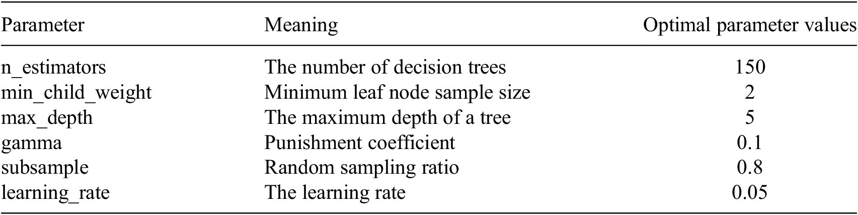
To ensure the reliability of the predictive results and to avoid potential overestimation of model performance, careful attention was paid to the selection and tuning of XGBoost hyperparameters in this study. As the present work addresses a regression prediction problem, the XGBRegressor module was adopted for model construction, and a systematic hyperparameter optimization procedure was conducted to achieve a balanced trade-off between predictive accuracy and model complexity. In the hyperparameter optimization process, a two-stage tuning strategy combining random search and grid search was employed. Initially, based on parameter ranges defined according to prior studies and empirical experience, random search was applied to key hyperparameters—including learning_rate, max_depth, min_child_weight, subsample, gamma, and n_estimators—to rapidly identify promising regions in the parameter space with favorable model performance. Subsequently, the parameter ranges were further narrowed, and a grid search was conducted to systematically evaluate candidate parameter combinations in order to obtain stable and reproducible optimal configurations. The performance of each parameter combination was assessed using multiple evaluation metrics on the testing set, including R2, RMSE, and MAE, and configurations leading to unstable performance or excessive model complexity were excluded. The final hyperparameter selection was not based solely on maximizing a single evaluation metric, but rather on a comprehensive consideration of predictive accuracy, generalization stability, and model interpretability. The optimized XGBoost model adopts relatively shallow tree depths, a moderate learning rate, and subsampling strategies, which effectively constrain model complexity while preserving strong nonlinear learning capability. Combined with the bridge-wise training–testing split strategy, this tuning approach ensures that the high prediction accuracy reported in this study reflects genuine model generalization rather than overfitting to the training data. The final optimal hyperparameter configuration is summarized in Table 3. This tuning strategy not only improves search efficiency but also effectively controls model complexity, thereby reducing overfitting risk and enhancing generalization stability on unseen bridge samples.
Key parameter statistics of the XGBoost model

4.4 Analysis of the prediction effects of different models
The XGBoost ensemble learning algorithm excels in handling complex nonlinear relationships, demonstrating superior performance in regression prediction compared to traditional models such as SVR and RF (Ma et al., Reference Ma, Wang, Zhao, Xiao, Xie and Feng2023). This study constructed two XGBoost models based on the open-source Python software Anaconda, designed specifically for predicting beam crack parameters (MCW and CD) in small- and medium-span hollow slab bridges. Evaluating model performance is a critical step in the development of machine learning models. Therefore, selecting evaluation metrics that comprehensively assess model performance is of paramount importance (Nie et al., Reference Nie, Zhang, Hou, du, Zhao, Xue, Lin, Cao and Wang2025).
Three evaluation metrics were selected: (1) R2 (coefficient of determination), (2) RMSE (root mean square error), and (3) MAE (mean absolute error). The value range of R2 extends from negative infinity to 1; values closer to 1 indicate superior model performance. Both RMSE and MAE have value ranges within [0, ∞). Smaller values for these metrics indicate that predictions are closer to the actual values, signifying higher predictive accuracy and, thus, better model quality. The calculation formulas for these metrics are as follows:
 $$ {\mathrm{R}}^2=1-\frac{\mathrm{SSE}}{\mathrm{SST}}=1-\frac{\sum \limits_{i=1}^n{\left({y}_i-{\hat{y}}_i\right)}^2}{\sum \limits_{i=1}^n{\left({y}_i-\overline{y}\right)}^2} $$
 $$ \mathrm{RMSE}=\sqrt{\mathrm{MSE}}=\sqrt{\frac{1}{n}\sum \limits_{i=1}^n{\left({y}_i-{\hat{y}}_i\right)}^2} $$
 $$ \mathrm{MAE}=\frac{1}{n}\sum \limits_{i=1}^n\left|\left({y}_i-{\hat{y}}_i\right)\right| $$
where $ n $
denotes the number of samples,
$ n $
denotes the number of samples, $ {y}_i $
represents the actual value,
$ {y}_i $
represents the actual value, $ \overline{y} $
signifies the mean of the actual sample values, and
$ \overline{y} $
signifies the mean of the actual sample values, and $ {\hat{y}}_i $
denotes the predicted value. SSE (Sum of Squared Errors) quantifies the deviation between the predicted and actual sample values, serving as an indicator of the model’s goodness of fit. SST (Total Sum of Squares) represents the deviation between the actual values and their mean, characterizing the total variation in the data. MAE stands for Mean Absolute Error.
$ {\hat{y}}_i $
denotes the predicted value. SSE (Sum of Squared Errors) quantifies the deviation between the predicted and actual sample values, serving as an indicator of the model’s goodness of fit. SST (Total Sum of Squares) represents the deviation between the actual values and their mean, characterizing the total variation in the data. MAE stands for Mean Absolute Error.
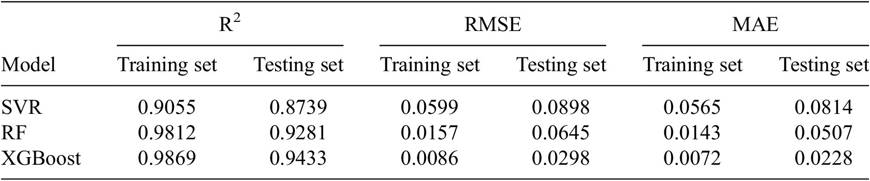
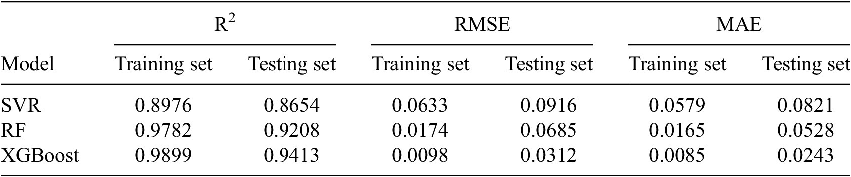
Following the aforementioned procedures and multiple iterations of model training, the evaluation metrics for the beam crack parameter prediction models based on the three machine learning algorithms, that is, SVR, RF, and XGBoost, were obtained, as presented in Tables 4 and 5. Tables 4 and 5 demonstrate that the XGBoost model achieved R2 values of 0.9869 and 0.9433 on the training and testing sets, respectively, for predicting MCW. The RF model attained R2 values of 0.9812 and 0.9281 on the training and testing sets, respectively, for the same prediction task. These values are significantly higher than those of the SVR model, which achieved 0.9055 and 0.8739 on the training and testing sets. Similarly, for predicting CD, the XGBoost model yielded R2 values of 0.9899 and 0.9413 on the training and testing sets, respectively. The RF model reached R2 values of 0.9782 and 0.9208 on the training and testing sets. These results are also markedly superior to the SVR model’s corresponding values of 0.8976 and 0.8654. In summary, the coefficient of determination (R2) of the XGBoost model on the testing set exhibited improvements of 8.35 ± 0.45% and 1.9 ± 0.3% compared to the SVR and RF models, respectively. This indicates that the XGBoost model delivers superior predictive fitting performance.
Prediction accuracy metrics for MCW by different models

Prediction accuracy metrics for CD by different models

Furthermore, regarding prediction error, the XGBoost model achieved RMSE values of 0.0086 and 0.0298 on the training and testing sets, respectively, for predicting MCW, and 0.0098 and 0.0312 for CD. These RMSE values are consistently lower than those obtained by the other two models (SVR and RF) on both the training and testing sets. Similarly, for MAE, the XGBoost model attained values of 0.0072 and 0.0228 on the training and testing sets for MCW prediction, and 0.0085 and 0.0243 for CD prediction. These MAE values are also consistently lower than those recorded by both the RF and SVR models on the training and testing sets. Consequently, the XGBoost model demonstrates optimal performance and yields predictions closest to the actual values.
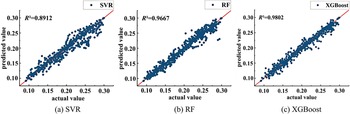
Figures 5 and 6 illustrate the fitting performance between predicted and actual values across the full dataset for the aforementioned models, respectively. It is evident that, for both MCW and CD predictions, the predicted values from the SVR and RF models exhibit a relatively scattered distribution overall. In contrast, the predicted values generated by the XGBoost model are clustered more tightly. A scatter plot distribution that clusters more closely around the linear trend line indicates superior predictive performance of the model. Regarding the evaluation metric R2, for MCW prediction on the full dataset, the SVR and RF models achieved R2 values of 0.8992 and 0.9076, respectively, both lower than the XGBoost model’s 0.9782. Similarly, for CD prediction on the full dataset, the SVR and RF models attained R2 values of 0.8912 and 0.9667, respectively, both falling below the XGBoost model’s 0.9802. Therefore, the prediction trends of the XGBoost model developed in this study align more closely with the actual values, further demonstrating its enhanced capability for nonlinear fitting.
Prediction fitting of MCW on the full dataset using different models.

Prediction fitting of CD on the full dataset using different models.

Figures 7 and 8 depict the prediction curves of the three distinct models based on the 20% testing set. Analysis of Figures 7 and 8 reveals that, for both the prediction of MCW and CD, the predicted values generated by the XGBoost model exhibit closer proximity to the actual values. This further demonstrates the effectiveness and feasibility of this model in predicting crack parameters.
Prediction curves of MCW by different models on the test dataset.

Prediction curves of CD by different models on the test dataset.

Although the sample size adopted in this study is relatively limited from a general machine learning perspective, the results presented in this section indicate that the proposed model still exhibits strong predictive accuracy, fitting capability, and generalization performance. This can be attributed to several key factors. First, the XGBoost model inherently incorporates multiple regularization mechanisms, including tree depth constraints, minimum child weight, and penalty terms, which effectively control model complexity and reduce the risk of overfitting under small-sample conditions. Second, a rigorous dataset splitting strategy was employed, ensuring that all samples from the same bridge were assigned to the same subset, and that bridges included in the testing set were completely unseen during the training phase. Under this strict bridge-wise separation scheme, the predictive performance on the testing set remains close to that on the training set, indicating stable generalization rather than overfitting. These results demonstrate that the moderate sample size does not significantly compromise the reliability of the proposed model and that the XGBoost-based framework is capable of achieving robust generalization and accurate prediction for bridge crack parameters even under limited data conditions.
4.5 Future crack evolution prediction
To further verify the effectiveness and reliability of the proposed model in predicting crack development in highway bridges, this section conducts a forward-looking crack evolution analysis based on the available dataset, with particular emphasis on the temporal generalization capability of the XGBoost model. The objective is to examine whether the model can effectively predict future crack evolution trends relying solely on historical information.
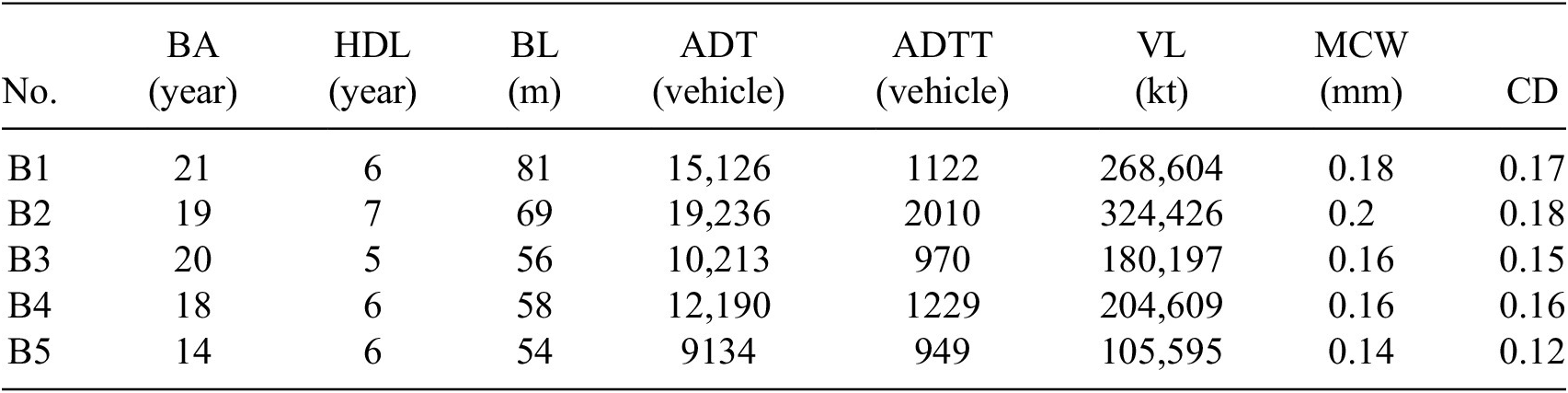
In this analysis, five representative bridges with multi-year continuous inspection records were selected from the testing set, and their basic crack information is summarized in Table 6. For each selected bridge, inspection and monitoring data from the early service period were used as model inputs to predict the future development of main beam crack parameters, including MCW and CD, over a 5-year horizon. Specifically, historical data from the initial inspection years were employed to forecast crack evolution over the subsequent 1–5 years, thereby simulating realistic bridge management scenarios in which future deterioration states are assessed based on currently available information.
Basic information on bridges used for future crack evolution prediction

Note. The bridge age reported in the table refers to the service age of each bridge at the prediction initiation year. As the most recent inspection year for all five bridges is 2024, crack development predictions are conducted for the period from 2025 to 2029 in this study. The column header “HDL” is an abbreviation for historical data length, which denotes the time span of continuous historical inspection records used for future crack evolution prediction for each bridge. Due to space limitations, only selected key feature variables closely related to crack development are listed in the table to illustrate the basic characteristics of the prediction targets. Other environmental factors and structural parameters are not individually reported but were all incorporated as input variables in the model training and prediction process.
In future crack evolution prediction, the updating of input variables during the prediction horizon strictly follows their physical meanings and statistical definitions in the original dataset. BA is calculated as the difference between the prediction year and the bridge construction (or opening-to-traffic) year, and therefore increases by one year at each prediction step. For traffic-related variables, ADT and ADTT are extrapolated through linear interpolation based on historical inspection and monitoring records, representing reasonable future variations in traffic demand.
It should be emphasized that the VL variable in this study does not represent an instantaneous or annual indicator, but rather a cumulative traffic load since the bridge was opened to traffic. Accordingly, during future crack evolution prediction, VL is updated in an accumulative manner rather than being held constant at the prediction initiation year. Specifically, the VL value for a given prediction year is obtained by adding the newly accumulated traffic load of that year to the cumulative value of the previous year. The annual increment of traffic load is estimated based on the corresponding truck traffic level for that year in combination with representative VL statistics derived from historical data, ensuring consistency between the prediction-stage VL calculation and its original data definition. This setting enables the model to capture the long-term cumulative effects of traffic loading on crack development.
Structural attributes such as bridge length are treated as time-invariant during the prediction period, while other environmental and auxiliary variables are fixed at their most recent recorded values or historical averages. Under these prediction settings, the proposed model is able to reasonably characterize the combined influence of increasing BA and cumulative traffic loading on crack evolution, while avoiding excessive extrapolation of uncertain future inputs. Consequently, the predicted MCW and CD provide forward-looking estimates of crack development trends for the period from 2025 to 2029, supporting preventive bridge maintenance and management decision-making. The predicted crack development trends of the five bridges over the next 5 years, based on the XGBoost model, are shown in Figure 9.
Predicted crack evolution of five representative bridges over the next 5 years.

Figure 9 presents the predicted evolution of CD and MCW for five representative bridges over the period from 2025 to 2029. As shown in the figure, both crack indicators exhibit overall increasing trends with time for all bridges, which is consistent with the expected cumulative deterioration behavior of reinforced concrete beam bridges under sustained traffic loading and environmental exposure. No abrupt fluctuations or unrealistic trend reversals are observed, indicating that the proposed model produces physically reasonable long-term predictions.
For CD, gradual increases are observed across all bridges, while the growth rates differ among bridges. Bridges subjected to higher traffic demand and VL (e.g., B2 and B1) exhibit relatively faster increases in CD, whereas bridges with lower traffic levels (e.g., B5) show more moderate growth. This differentiation suggests that the model is able to capture the long-term cumulative influence of traffic-related factors on crack propagation rather than merely extrapolating short-term fluctuations.
A similar trend is observed for MCW. MCW increases steadily with prediction year for all bridges, with higher absolute values and steeper growth rates generally corresponding to bridges with heavier traffic loading and larger cumulative VL. The predicted MCW trajectories remain smooth and continuous, without unrealistic jumps, indicating stable temporal behavior of the model under forward extrapolation.
Overall, the predicted crack evolution curves demonstrate that the proposed XGBoost-based framework is capable of extending learned deterioration patterns beyond the historical observation period. The consistency of the predicted temporal trends with engineering expectations, together with the reasonable differentiation among bridges with different traffic and loading characteristics, provides strong evidence of the model’s temporal generalization ability. These results indicate that the proposed approach does not merely fit historical inspection data, but can effectively project crack development trends into future service years. Moreover, the forward-looking prediction results further confirm the engineering applicability of the XGBoost model and demonstrate that, even under a relatively small sample size, the model is able to maintain good temporal generalization performance and strong predictive capability, thereby supporting its potential use for proactive bridge maintenance and management.
5. Interpretability analysis
5.1. SHAP
Machine learning models are typically categorized into black-box models and white-box models (Gao et al., Reference Gao, Tian and Liu2025; Liu et al., Reference Liu, Kergus, Claveau, Philippe and Lacarrière2025). Black-box models include RF, SVR, XGBoost, and LightGBM (Light gradient boosting machine), among others. The majority of existing machine learning models are black-box models. However, the primary limitation of black-box models lies in their complex internal mechanisms, which make it difficult for researchers to interpret the prediction results, thereby constraining the credibility and persuasiveness of the outcomes. In contrast, white-box models (interpretable machine learning models) address the issue of low persuasiveness associated with black-box model results. While most white-box models offer high interpretability, their relatively lower prediction accuracy often makes them insufficient for meeting research requirements. White-box models can be interpreted from two distinct perspectives, that is, intrinsic and post hoc. Certain intrinsically interpretable machine learning models, such as GAMI-Net, achieve excellent predictive performance while simultaneously providing reasonable explanations for their results. However, a significant drawback of GAMI-Net is its computationally intensive training process, and its high predictive accuracy and strong interpretability come at the cost of substantial time investment, resulting in lower prediction efficiency. Nevertheless, predictive results from black-box models can be subjected to post hoc interpretation using analytical methods grounded in game theory. Among these, SHAP serves as a post hoc interpretation method based on the principles of game theory (Lundberg et al., Reference Lundberg, Erion, Chen, DeGrave, Prutkin, Nair, Katz, Himmelfarb, Bansal and Lee2020; Ma et al., Reference Ma, Wang, Wang, Guo and Feng2023; Zheng et al., Reference Zheng, Hu and Yu2024). The model calculates the marginal contributions (Shapley values) of individual input parameters and their interaction terms. These values quantify the extent of influence each input parameter and its interactions exert on the output parameter, thereby achieving the goal of post hoc explanation. The expression for calculating the SHAP value is given by:
 $$ {\phi}_i=\sum \limits_{S\subseteq N(i)}\frac{\left|S\right|!\left(M-\left|S\right|!-1\right)}{M!}\left[{f}_x\left(S\cup \left\{i\right\}\right)-{f}_x(S)\right] $$
where $ {\phi}_i $
denotes the contribution of the
$ {\phi}_i $
denotes the contribution of the $ \mathrm{i} $
-th feature,
$ \mathrm{i} $
-th feature, $ \mathrm{N} $
represents the set of all features,
$ \mathrm{N} $
represents the set of all features, $ M $
signifies the total number of features, and
$ M $
signifies the total number of features, and $ \mathrm{S} $
denotes a subset of features used for a given prediction. The terms
$ \mathrm{S} $
denotes a subset of features used for a given prediction. The terms $ {f}_x\left(S\cup \left\{i\right\}\right) $
and
$ {f}_x\left(S\cup \left\{i\right\}\right) $
and $ {f}_x(S) $
represent the model outputs with and without the
$ {f}_x(S) $
represent the model outputs with and without the $ i $
th feature, respectively (Chen et al., Reference Chen, Yue, Wang, Wang, Xie, Tian, Zhang and Jia2025). SHAP approximates complex models through an additive combination of multiple linear models. The explanation model
$ i $
th feature, respectively (Chen et al., Reference Chen, Yue, Wang, Wang, Xie, Tian, Zhang and Jia2025). SHAP approximates complex models through an additive combination of multiple linear models. The explanation model $ g\left({z}^{\prime}\right) $
for an output with
$ g\left({z}^{\prime}\right) $
for an output with $ M $
features is defined as the linear sum of input variables, that is
$ M $
features is defined as the linear sum of input variables, that is
 $$ g\left({z}^{\prime}\right)={\phi}_0+\sum \limits_{i=1}^M{\phi}_i{z}_i^{\prime } $$
where $ {\phi}_0 $
is the prediction result without any feature values;
$ {\phi}_0 $
is the prediction result without any feature values; $ {\phi}_i $
is the Shapley value for the
$ {\phi}_i $
is the Shapley value for the $ i $
th feature;
$ i $
th feature; $ {z}_i^{\prime } $
indicates that it equals 1 when the
$ {z}_i^{\prime } $
indicates that it equals 1 when the $ i $
th feature is selected, and 0 otherwise.
$ i $
th feature is selected, and 0 otherwise.
5.2. Feature importance analysis
Section 4 establishes a black-box model for crack parameters in single-span bridge main beams based on XGBoost, subsequently determining the optimal hyperparameter combination and training set proportion for the model. This subsection employs the SHAP method to provide post hoc interpretation for the predictions generated by the XGBoost model.
Figure 10 presents the feature importance ranking plot for the output parameter of MCW, derived from the explainable machine learning model, with the abscissa representing the SHAP value magnitude of each feature and the ordinate listing the features influencing the MCW in the main beams. As illustrated in Figure 10, VL, ADTT, BA, and ADT constitute the most significant factors influencing the MCW in single-span bridge main beams, collectively contributing 63.8% to its variation. The influence of MS and S is also notable, whereas MR, BL, and APC exhibit less significant impact on the MCW in single-span bridges.
Feature importance ranking for MCW.

Figure 11 displays the feature importance ranking plot for the output parameter of CD, derived from the explainable machine learning model, with the abscissa representing the magnitude of the SHAP values for each feature parameter, and the ordinate listing the feature parameters influencing the CD in the main beams. As indicated in Figure 11, VL, ADTT, BA, and ADT constitute the most significant factors affecting the CD in single-span bridge main beams, collectively accounting for 59.1% of its variation. The influence of MS and EHT is also notable, whereas BL, MR, and APC exhibit minimal impact on the CD in single-span bridges.
Feature importance ranking for CD.

6. Conclusions
This study developed an interpretable machine learning framework for predicting crack propagation in small- and medium-span beam bridges. The main conclusions can be summarized as follows.
-
(i) The XGBoost model demonstrates superior predictive performance for crack parameters with R2 values of 0.9433 for MCW and 0.9413 for CD, significantly outperforming SVR and RF models. In addition, the proposed model achieves significant improvements in prediction accuracy, reducing the root mean square error (RMSE) by up to 66.8% and the mean absolute error (MAE) by up to 72% compared with the SVR and RF models.
-
(ii) By predicting the crack parameters of five in-service bridges over a 5-year horizon, the effectiveness and reliability of the XGBoost model in highway bridge crack development prediction are verified. The results demonstrate that the proposed model exhibits strong temporal generalization capability and practical engineering applicability, providing more targeted decision support for preventive bridge maintenance.
-
(iii) SHAP analysis reveals that VL (19.7%), daily truck traffic, BA, and total traffic volume are the most influential factors, collectively contributing 61.45 ± 2.35% to crack development.
-
(iv) Excessive traffic loading and aging are identified as the dominant drivers of crack propagation in beam bridges, providing critical insights for targeted maintenance strategies.
-
(v) The interpretable machine learning framework effectively bridges the gap between prediction accuracy and model transparency, offering both reliable crack forecasting and clear identification of underlying deterioration mechanisms.
Acknowledgments
The authors acknowledge the financial support from the National Natural Science Foundation of China (No. 52478310) and the Enterprise R&D Special Project of Tiankai Higher Education Innovation Park (No. 23YFZXYC00026). In addition, the authors would like to thank China Communications Construction First Highway Engineering Bureau Co., Ltd. for supplying bridge inspection reports and monitoring information.
Data availability statement
Supplementary material containing the data utilized in this work can be found at https://www.researchgate.net/publication/395459442_dataset.
Author contribution
Conceptualization-Equal: M.H.; Conceptualization-Lead: D.L., H.H.; Methodology-Equal: Z.Z., J.S.; Methodology-Lead: M.H.; Resources-Lead: F.D.; Supervision-Lead: D.L.; Validation-Lead: M.H., F.D.; Writing – Original Draft-Lead: M.H.; Writing – Review & Editing-Equal: D.L., J.S.; Writing – Review & Editing-Lead: F.D.
Competing interests
The authors declare that they have no known competing financial interests or personal relationships that could have appeared to influence the work reported in this paper.


 Open access
Comments
No Comments have been published for this article.