


1. Introduction
In the European Alps, cold glaciers suitable for ice-core drillings with a paleoclimate objective are confined to very few high summit regions (Haeberli, Reference Haeberli1976; Lliboutry and others, Reference Lliboutry, Briat, Creseveur and Pourchet1976; Suter and others, Reference Suter, Laternser, Haeberli, Frauenfelder and Hoelzle2001; Hoelzle and others, Reference Hoelzle, Darms, Lüthi and Suter2011). Suitable drill sites in Central Europe are in general located above 4000 m a.s.l., because lower elevation sites experience too much melt to preserve the chemical and physical signatures of interest. In the Alps, drill sites are situated in vicinity not only to anthropogenic emission sources but also to a dense network of instrumental observations and other complementary climate archives (e.g. tree rings), albeit at lower elevations. Alpine summit glaciers have a small spatial extent and intermediate to shallow ice thicknesses (in most cases ≤100 m). As maximum ages are mostly confined to the Holocene or less, temporal changes in basal topography or divide migration are likely minimal. This means that these sites are relatively constrainable targets for modeling compared to more complex regions such as in Antarctica or Greenland. However, summit glaciers also traditionally exhibit complex3-D flow fields, which must be accounted for to properly constrain ages from an ice-core record (Lüthi and Funk, Reference Lüthi and Funk2000). Coupled with ice flow, spatial and temporal variations in net snow accumulation can introduce distinctive biases that must be considered when interpreting ice-core proxies (Bohleber, Reference Bohleber2019).
This set of problems applies to Colle Gnifetti (CG, 4450 m a.s.l.), where a number of full-depth ice cores have been extracted since the 1980s (Wagenbach and others, Reference Wagenbach, Bohleber and Preunkert2012). CG forms a glacier saddle between the peaks Signalkuppe and Zumsteinspitze in the Monte Rosa massif with a horizontal extent of a few 100 m and a maximum ice thickness of 120 m. The glaciological features of this ice-core drill site are thoroughly described in the literature (e.g. Wagenbach and others, Reference Wagenbach, Bohleber and Preunkert2012, and references therein). The glacier geometry has been in steady state from at least the 1890s to the end of the 20th century (Haeberli and others, Reference Haeberli, Schmid and Wagenbach1988; Wagner, Reference Wagner1996; Lüthi, Reference Lüthi2000). Basal ice temperatures ranging between −12°C and −13°C ensure that the glacier is frozen to bedrock, although a recent warming trend is evident in englacial temperatures (Haeberli and Funk, Reference Haeberli and Funk1991; Hoelzle and others, Reference Hoelzle, Darms, Lüthi and Suter2011; Bauder and others, Reference Bauder2017). A distinctive characteristic of CG is the exceptionally low and variable snow accumulation rates (~0.15–1.2 m w.e. a−1) due to wind erosion, as shown by direct measurements of snow accumulation, ground-penetrating radar (GPR) profiles and ice cores (Alean and others, Reference Alean, Haeberli and Schädler1983; Bohleber and others, Reference Bohleber, Wagenbach, Schöner and Böhm2013; Konrad and others, Reference Konrad, Bohleber, Wagenbach, Vincent and Eisen2013). Moreover, the impact of wind erosion is evident considering that, in the north-facing flank of the glacier, net accumulation can be lower by up to a factor of nine than the climatologic precipitation rate (Bohleber and others, Reference Bohleber, Wagenbach, Schöner and Böhm2013). Intrinsically tied to this, CG offers the opportunity to retrieve ice-core records on the multi-centennial to millennial time scale (Wagenbach, Reference Wagenbach1992). Constraining the uncertainty in ice-core chronologies beyond the first few hundred years is a challenge at CG, but recent advances in micro-radiocarbon measurements and high-resolution annual layer counting have reduced these uncertainties (Jenk and others, Reference Jenk2009; Hoffmann and others, Reference Hoffmann2018; Bohleber and others, Reference Bohleber2018). In particular, these latest advances in dating have paved the way for exploration of the CG time series over longer time scales, e.g. the last millennium and beyond (Thevenon and others, Reference Thevenon, Anselmetti, Bernasconi and Schwikowski2009; More and others, Reference More2017; Bohleber and others, Reference Bohleber2018; Loveluck and others, Reference Loveluck2018).
At the same time, the interpretation of the deep and old ice-core layers calls for improved knowledge of the accumulation conditions upstream of the drilling site. At CG, wind erosion is counteracted by insolation-driven snow consolidation, and thus snow removal by wind is most efficient at hill-shaded slopes and during winter time (Wagenbach, Reference Wagenbach1992). As a result, snow accumulation on its north-facing flank is systematically lower and more summer-biased compared to the center of the saddle (Schöner and others, Reference Schöner, Auer, Böhm, Keck and Wagenbach2002; Bohleber and others, Reference Bohleber, Wagenbach, Schöner and Böhm2013). This means that the inflow of ice from the slope catchment area can produce systematic biases in the average levels of stable water isotopes and impurities, especially for the deeper layers in ice cores drilled toward the saddle (Wagenbach, Reference Wagenbach1992; Keck, Reference Keck2001). In particular, if the amount of preserved winter snow decreases upstream of a drill site, the respective long-term mean in the ice core will be biased toward less isotope depletion (shift toward the summer levels). In contrast, if winter snow increases upstream, the long-term mean will be shifted toward more isotope depletion. This trend is not a climatic signal, however, and is referred to as the ‘upstream effect’ (Bohleber, Reference Bohleber2019, e.g. Fig. 5 therein). A typical investigation of upstream effects relies on a shallow ice-core series along a flowline to study the relative contribution of winter- and summer-related signals in the respective impurity levels. However, this approach is mostly feasible at high accumulation sites like Col du Dome (Mont Blanc) where a bias of ~20% was found for nitrate, sulfate, and calcium and 30% for ammonium, depending on the magnitude of their seasonality (Preunkert and others, Reference Preunkert, Wagenbach, Legrand and Vincent2000). At CG, the spatial variability of seasonal signals at shallow depths suggest that the upstream effect in deep ice-core layers could be as large as 100% (Preunkert and others, Reference Preunkert, Wagenbach, Legrand and Vincent2000). However, the CG site still awaits a dedicated assessment of the upstream effect (Keck, Reference Keck2001), a need recognized with new urgency in view of the latest dating advances (Bohleber and others, Reference Bohleber2018). Because any quantitative investigation (and correction) of the upstream effect critically relies on an identification and characterization of the upstream catchment area, the use of numerical models to study the ice flow becomes imperative.
Advanced numerical ice-flow models provide invaluable information regarding upstream source regions and dating constraints and have become indispensable instruments to investigate the dynamics of small scale glaciers (e.g. Lüthi and Funk, Reference Lüthi and Funk2000; Zekollari and others, Reference Zekollari, Huybrechts, Fürst, Rybak and Eisen2013; Gilbert and others, Reference Gilbert, Gagliardini, Vincent and Wagnon2014a). At CG, numerous ice-flow modeling studies have been conducted since the late 1980s to investigate the flow dynamics of the firn saddle and to support ice-coring projects. The flow model proposed in Haeberli and others (Reference Haeberli, Schmid and Wagenbach1988), the first of these modeling studies, was based on a simple 2-D parallel slab approximation and assumed viscous flow of pure glacier ice. Wagner (Reference Wagner1996) established the first 3-D finite element (FE) ice-flow model of CG. Later studies used a constitutive equation accounting for firn compressibility to reproduce observed surface velocities, density and temperature profiles, and provided dating results in agreement with most of the ice-core chronologies available at that time (Lüthi, Reference Lüthi2000; Lüthi and Funk, Reference Lüthi and Funk2000, Reference Lüthi and Funk2001). As an alternative approach, Konrad and others (Reference Konrad, Bohleber, Wagenbach, Vincent and Eisen2013) used the parallel slab approximation (2-D), but with an additional parameter accounting for transversal ice fluxes and constraints from various glaciological and geophysical datasets. Notably, ice-flow modeling studies require adequate knowledge of the glacier geometry. To provide this essential boundary condition, geophysical investigations were extensively conducted at CG since the 1980s (Haeberli and others, Reference Haeberli, Schmid and Wagenbach1988), providing information on bedrock topography, internal structure (e.g. reflections of isochronic origin) and accumulation distribution (Eisen and others, Reference Eisen, Nixdorf, Keck and Wagenbach2003; Böhlert, Reference Böhlert2005; Bohleber, Reference Bohleber2011; Konrad and others, Reference Konrad, Bohleber, Wagenbach, Vincent and Eisen2013).
In this work, we present a new full Stokes ice-flow model of the CG glacier saddle using Elmer/Ice (Gagliardini and others, Reference Gagliardini2013). We respond to the need for new model development and application at CG, and specifically target the source region investigation of two new ice cores drilled on the same flowline in 2005 and 2018. Both cores offer ice-core chronologies on the millennial time scale (Bohleber and others, Reference Bohleber2018). Our target is therefore different from the one in Lüthi and Funk (Reference Lüthi and Funk2000), whose focus area was the western part of the glacier with the drill sites of 1982 and 1995. Compared to previous modeling studies, our model is supported by a larger amount of direct observations (see Section 3), especially concentrated in our focus area, and better constrained ice-core chronologies (Bohleber and others, Reference Bohleber2018; Hoffmann and others, Reference Hoffmann2018). Accordingly, our new model of CG is used for (a) calculating backward trajectories from the existing drill sites, which is required to evaluate potential upstream effects, and (b) developing a depth-age field of the glacier, to support and supplement existent ice-core chronologies based on experimental methods.
2. Ice-flow model
2.1. Governing equations
2.1.1. Momentum, mass and internal energy conservation
The full Stokes ice-flow model is based on three intimately coupled field equations (Greve and Blatter, Reference Greve and Blatter2009): the Stokes equation (momentum balance), the continuity equation (mass conservation) and the temperature equation (conservation of internal energy). In this work, we account for internal energy conservation adopting the enthalpy formulation proposed by Aschwanden and others (Reference Aschwanden, Bueler, Khroulev and Blatter2012) and implemented in Elmer/Ice by Gilbert and others (Reference Gilbert, Gagliardini, Vincent and Wagnon2014a):

with H the enthalpy variable, $\bi {\vec {v}}$ the flow velocity, κ the enthalpy diffusivity, ρ the firn/ice density, σ the Cauchy stress tensor and ${\dot {\bi \epsilon }}$
 the strain-rate tensor. Definition and dependencies of the enthalpy variable H and enthalpy diffusivity κ can be found in Gilbert and others (Reference Gilbert, Gagliardini, Vincent and Wagnon2014a). The last two terms in Eqn (1) are energy source terms due to internal deformation and refreezing of meltwater (Q lat).
2.1.2. Free-surface equation
The evolution of the glacier surface is described by the free-surface equation (Greve and Blatter, Reference Greve and Blatter2009):

where s(x, y, t) represents the surface elevation, v sx, v sy and v sz the three components of the surface velocity ${\vec{\bi v}_{\rm {s}}} (x, y, t)$ , and $\dot {b}_{\rm s}(x, y, t)$
 the ice-equivalent surface mass balance.
2.1.3. Dating equation
The dating equation calculates the age of the ice according to a prescribed velocity field. The age of the ice is considered as a scalar quantity, which is advected with the flow (Zwinger and others, Reference Zwinger, Greve, Gagliardini, Shiraiwa and Lyly2007; Gagliardini and others, Reference Gagliardini2013):

with $\cal {A}$ the age variable and $\bi {\vec {v}}$
 the velocity field.
2.1.4. Constitutive equation
The relation between stress and strain-rate tensor is described by a constitutive equation accounting for firn compressibility (Gagliardini and Meyssonnier, Reference Gagliardini and Meyssonnier1997; Lüthi and Funk, Reference Lüthi and Funk2000; Zwinger and others, Reference Zwinger, Greve, Gagliardini, Shiraiwa and Lyly2007):

where $\dot {\epsilon }_{ij}$ are the components of the strain-rate tensor ${\dot{\bi \epsilon}}$
 and τij the components of the deviatoric stress tensor τ (δij is the Kronecker delta). The fluidity parameter B is temperature dependent and is derived from the creep parameter A of Glen's law (B=2A). Further, n is the creep exponent, p is the isotropic pressure and σD is the stress invariant ($\sigma _D^2=a\tau ^2+bp^2$
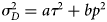 , with τ the second invariant of τ). The parameters a and b depend on the firn's relative density D = ρ/ρice. For high relative densities (D > 0.81), a and b are determined analytically (Duva and Crow, Reference Duva and Crow1994), whereas for lower relative densities (D ≤ 0.81) we use the parameterization proposed in Zwinger and others (Reference Zwinger, Greve, Gagliardini, Shiraiwa and Lyly2007). At firn densities approaching the ice density (D → 1), the parameters converge to a = 1 and b = 0, and Eqn (4) reduces to Glen's law (Cuffey and Paterson, Reference Cuffey and Paterson2010).
2.2. Boundary conditions
2.2.1. Mechanical boundary conditions
The lateral boundaries of the modeled glacier domain are represented in Figure 1 with thick black lines. The southern boundary is located below Signalkuppe and follows partly the course of a bergschrund. The ice upstream of the bergschrund is almost stagnant due to the reduced ice thickness. We therefore consider the bergschrund boundary as stress-free. Likewise, the eastern ice-cliff and the northern boundary are treated as stress-free. A large crevasse is visible along the western boundary of the modeling area. Where the crevasse is visible, the normal stress σn applied on this boundary is defined using a parameterization equivalent to the one used in Lüthi and Funk (Reference Lüthi and Funk2000):

with d the depth coordinate, d c the crevasse depth and κc the vertical stress gradient. In our study, we set the crevasse depth to d c = 30 m and the stress gradient to κc = 104 Pa m−1. Since direct measurements of the crevasse geometry are not available, those parameters are estimated comparing model results with surface velocities measured close to the KCS site. We assume that the glacier is frozen to the bedrock, therefore basal flow velocities are set equal to zero (no-slip condition). This assumption is supported by measurements showing basal temperatures between −12 and −13°C (Haeberli and Funk, Reference Haeberli and Funk1991; Hoelzle and others, Reference Hoelzle, Darms, Lüthi and Suter2011; Bauder and others, Reference Bauder2017).
North oriented areal imagery of the CG glacier saddle. The investigated area is partitioned into five sectors. Note the large ice cliff on the eastern boundary of the glacier, the bergschrund on the southern boundary and the large crevasse on the western boundary. Red dots indicate the position of ice cores considered in this work. Blue dots indicate the position of two additional boreholes, for which we exclusively consider the temperature measurements. Coordinates are in the official Swiss coordinate system (conversion to an international coordinate system available at https://www.swisstopo.admin.ch/en/maps-data-online/calculation-services/navref.html). Areal imagery from https://map.geo.admin.ch (here and in the next figures).

2.2.2. Thermodynamic boundary conditions
For the model spin-up (see Section 2.4) steady surface temperatures T s(x, y) are used as a boundary condition. The temperatures T s are estimated comparing model calculations with measured temperature profiles. At locations not constrained by temperature measurements (e.g. the northern half of the glacier), steady surface temperatures are roughly estimated considering surface aspect, which dominates over elevation differences, as suggested by measurements. As an example, the drill sites KCI and KCS (see Fig. 1) are located at almost the same altitude, but the estimated surface temperature at KCI is 0.3 K warmer than at KCS (see temperature profiles in Fig. 2). The horizontal spatial variability of the estimated temperatures T s is less than 1.0 K, which is about the range of horizontal variability of measured deep temperature profiles (Hoelzle and others, Reference Hoelzle, Darms, Lüthi and Suter2011).
Comparison of calculated (dashed lines with stars) and measured (solid lines with circles) temperature profiles. Different colors correspond to different times (both for measurements and model results). Note the different scales on the y-axis. The borehole locations are indicated in Figure 1. The system of the identification code assigned to each measurement is taken from Hoelzle and others (Reference Hoelzle, Darms, Lüthi and Suter2011). The first and last two digits indicate the year of drilling of the borehole and the year of the temperature measurement, respectively. The histogram in the bottom-right panel shows the deviations between modeled and measured temperatures below the depth of zero annual amplitude (ZAA-depth, ~20 m).

For the fully coupled transient simulations (see Section 2.4), we consider yearly-averaged atmospheric temperature anomalies T dev(t) as a function of time t since 1901 and the yearly-averaged amount of latent heat Q lat(t) released due to refreezing of surface meltwater. The space and time dependent surface enthalpy boundary condition is defined as follows:

where C p = 152.5 + 7.122 T is the temperature-dependent heat capacity (T in Kelvin; Yen, Reference Yen1981), T 0 is the reference temperature for enthalpy (here 200 K) and it is assumed that the yearly-averaged surface temperature (T s + T dev) does not reach the pressure melting-point temperature.
Air temperature anomalies T dev(t) are based on instrumental data recorded at weather stations located at the Regina Margherita Hut (4560 m a.s.l., operated by Arpa Piemonte, http://www.arpa.piemonte.gov.it), Gornergrat and Zermatt (respectively 3129 and 1638 m a.s.l., both operated by MeteoSchweiz, http://www.meteoschweiz.ch). Instrumental temperature data further back in time (until the year 1901) are taken from the Monte Rosa grid cell of the HISTALP database (5 × 5 arcmin2 grid; Auer and others, Reference Auer2007). Temperature anomalies are arbitrarily calculated with respect to the mean temperatures recorded after 1982 and the correlation between the different datasets is high. The T dev time series used as input for the model is obtained averaging over all available datasets (see Fig. 5.8 in Licciulli, Reference Licciulli2018). The data show an increase of atmospheric temperatures at CG of ~2°C since 1901.
The yearly-averaged amount of released latent heat Q lat(t) is estimated by applying a variation of the degree-day model used in Gilbert and others (Reference Gilbert2014b) and previously introduced by Hock (Reference Hock1999):

where T +(t) is the positive yearly-averaged daily-maximum air temperature and α the melt factor. We are interested in yearly-averaged quantities, since the simulations run with 1-year time steps. We found the best agreement between model calculations and measured englacial temperatures setting α = 1500 J kg−1 K−1 (constant in space and time, see Section 4.1.5).
At CG, the spatial distribution of basal heat fluxes is strongly influenced by the sun-exposed east and south face of Monte Rosa. We estimated basal heat fluxes comparing model calculations with measured temperature profiles (note that basal heat flux influences the slope of the temperature profile, therefore this estimation does not interfere with the estimation of T s). The basal heat flux estimated at the KCH site (43 mW m−2) is higher than that in the middle of the saddle (e.g. 30 mW m−2 at the KCS site). This is because KCH is not far from the south-exposed rock face below Signalkuppe. The KCI site is close to the Monte Rosa east face and shows enhanced basal heat flux as well (39 mW m−2). At locations without direct measurements the basal heat flux is roughly estimated considering the presence or absence of exposed slopes nearby. Our estimation ranges between 30 and 45 mW m−2 and is consistent with previous estimations for high-altitude glaciers in the Western Alps (Haeberli and Funk, Reference Haeberli and Funk1991; Lüthi and Funk, Reference Lüthi and Funk2001; Suter, Reference Suter2002).
2.3. Numerical implementation
The ice-flow model is implemented using the open-source FE software Elmer/Ice (Gagliardini and others, Reference Gagliardini2013). Among other applications, this software is widely used to investigate small-scale glaciers (e.g. Gagliardini and others, Reference Gagliardini, Gillet-Chaulet, Durand, Vincent and Duval2011; Gilbert and others, Reference Gilbert, Vincent, Gagliardini, Krug and Berthier2015). The mesh used to approximate the model geometry consists of 3088 nodes and 2505 trilinear hexahedrons. The 3-D mesh is extruded from a 2-D mesh of the footprint of the glacier, which has an horizontal resolution of 50 m. We use 16 extrusion layers, which are gradually more closely together approaching the glacier surface. The evolution of the density field is calculated selecting the bubbles stabilization method (Arnold and others, Reference Arnold, Brezzi and Fortin1984; Brezzi and others, Reference Brezzi, Bristeau, Franca, Mallet and Rogé1992; Baiocchi and others, Reference Baiocchi, Brezzi and Franca1993). This method was preferred to the discontinuous Galerkin method (Brezzi and others, Reference Brezzi, Marini and Süli2004), to avoid density oscillations, especially close to the model boundaries. The dating equation is solved with the Streamline Upwind Petrov-Galerkin stabilization method (Donea, Reference Donea1984; Hughes, Reference Hughes1987).
2.4. Calculation of the fully-coupled solution
The fully thermo-mechanically coupled flow solution is calculated partially following the approach presented in Gilbert and others (Reference Gilbert, Gagliardini, Vincent and Wagnon2014a). Based on geodetic observations (Haeberli and others, Reference Haeberli, Schmid and Wagenbach1988; Wagner, Reference Wagner1996; Lüthi, Reference Lüthi2000), we assume that the glacier geometry is in steady state, but we consider the effect of atmospheric temperature changes on englacial temperatures. For model spin-up, we combine a series of prognostic and diagnostic runs. First, a transient simulation is started to evolve velocity and density to a quasi-equilibrium state. Different from Gilbert and others (Reference Gilbert, Gagliardini, Vincent and Wagnon2014a), we keep the surface elevation constant and we do not force the glacier geometry with a prescribed mass balance. To ensure fast convergence, the prescribed initial density and temperature fields are chosen as realistic as possible and based on core observations (see Section 3.4). Afterward, the evolved velocity and density fields are used as input for a diagnostic simulation, where the temperature field is updated (using the steady surface temperatures T s(x, y) introduced in Section 2.2.2). The new temperature field is prescribed for a new transient simulation, where velocity and density field are further evolved. Transient and diagnostic simulations are iteratively repeated until all variables reach equilibrium. The solution of the model spin-up is used as initial condition for a transient simulation with changing surface enthalpy starting from 1901 (see Eqn (6) in Section 2.2.2). This step is necessary to reproduce the warming of englacial temperatures observed over the last decades. The simulation runs with time steps of 1 year.
2.5. Calculation of borehole inclination angles
Borehole deformation is calculated by post-processing the model output, assuming that the presence of the borehole does not influence macroscopic ice flow and that the investigated boreholes (KCC and KCI) were straight and vertical lines just after drilling. Calculations are performed using three different methods. The first method assumes internal deformation exclusively due to simple shear. In accumulation areas like CG, this is the case only far below the glacier surface, where compression becomes negligible. Neglecting horizontal gradients of velocity, the only non-zero strain components are $\dot {\epsilon }_{zx}=\dot {\epsilon }_{xz}=\partial v_x / \partial z$ (with z the vertical coordinate and x the horizontal flow direction). Hence, borehole inclination angles θ(z) are calculated as

with Δt the elapsed time after drilling.
The second method follows the procedure presented in Gudmundsson and others (Reference Gudmundsson, Bauder, Lüthi, Fischer and Funk1999) to calculate tilt curves from a given velocity field. However, differently from Gudmundsson and others (Reference Gudmundsson, Bauder, Lüthi, Fischer and Funk1999), we neglect horizontal gradients of velocity, since at CG horizontal velocities are small and, with respect to those, the elapsed time after drilling is short. In other words, borehole advection is small and variations of the velocity field over such a short length scale are negligible. The third method considers the borehole as an ensemble of particles, which are used as passive tracers of the flow field. The particles are initially positioned along a straight vertical line. Afterward, particles' paths are calculated using the ParticleDynamics-Solver available in Elmer. Finally, inclination angles are determined by fitting the positions of all particles after a certain time Δt using a piecewise linear function.
3. Constraints from direct observations
The CG saddle is divided into five sectors (see Fig. 1). Sector 1 includes the drilling sites and is well covered by field measurements. Sectors 2 and 3 contain the eastern ice cliff and the large crevasse at the western boundary of the saddle, respectively. Sector 4 corresponds to the northern half of the glacier, where the majority of the field data was made available by Wagner (Reference Wagner1996) and Lüthi (Reference Lüthi2000). Sector 5 covers the southernmost part of the glacier.
3.1. Surface and bedrock topography
The glacier input geometry is constrained by direct observations. At locations where field measurements are sparse or absent, surface and bedrock altitudes are manually estimated to: (i) minimize the discrepancy between observed and calculated surface velocity fields, (ii) minimize the discrepancy between observed and calculated surface accumulation and (iii) make the glacier thickness consistent with the length of extracted ice cores. Uncertainties arising from this procedure are included in the results (see Sections 4.2.1 and 4.2.2).
The surface topography of sector 1 is cubically interpolated from direct measurements taken between 2014 and 2016, whereas the glacier bed is cubically interpolated from GPR profiles available from previous studies (Eisen and others, Reference Eisen, Nixdorf, Keck and Wagenbach2003; Bohleber, Reference Bohleber2011; Konrad and others, Reference Konrad, Bohleber, Wagenbach, Vincent and Eisen2013). Due to lack of direct measurements, surface and bedrock topography of sector 2 are estimated following the criteria (i) to (iii) above. This estimation is also supported by photographs of the ice cliff. Surface and bedrock topography of sectors 3 and 4 are based on DEMs used in previous modeling studies (Wagner, Reference Wagner1996; Lüthi, Reference Lüthi2000), with few adjustments at the glacier boundaries (criteria (i) to (iii)). Finally, surface and bedrock topography of sector 5 are estimated by photographs only, which does not significantly limit the accuracy of the model results (according to sensitivity studies, the geometry of sector 5 influences only marginally the flow of the rest of the glacier).
3.2. Horizontal surface velocity
Available surface velocity measurements are shown in Figure 3 and include: stake measurements performed on a regular grid in the central saddle area in the 1980s (Haeberli and others, Reference Haeberli, Schmid and Wagenbach1988); measurements of the period 1989–1990 conducted in the northern part of the glacier and in the region close to the western boundary (Wagner, Reference Wagner1996); measurements started in 1995 and 1998 along the flowline comprising the drill sites KCH, CC and KCS (Lüthi, Reference Lüthi2000; Lüthi and Funk, Reference Lüthi and Funk2000; Keck, Reference Keck2001); and measurements conducted within this study (2014–2016), focusing on the KCC-KCI area (Licciulli, Reference Licciulli2018).
(a) Horizontal surface velocities calculated at the mesh nodes (black arrows) and stake measurements (red arrows). (b) Ratio between calculated (v m) and measured (v s) vector magnitudes. (c) Deviations of the direction of the calculated velocity vectors from the measured flow directions.

3.3. Borehole inclination measurements
We measured borehole inclination angles at KCC and KCI in September 2016, i.e. 3 and 11 years after drilling, respectively (low accumulation and successive casing guaranteed access to the boreholes for several years). The measurements were performed using the DIgital BOrehole Sensor System (DIBOSS) (Ryser, Reference Ryser2014; Ryser and others, Reference Ryser2014). Results of the survey are presented in Figs 4a, b. Inclination angles are measured downward, letting the probe down from the top to the bottom of the borehole (blue squares), and upward (red squares). The positioning of the inclinometer probe inside the borehole should be parallel to the borehole walls. Although equipped with centralizers, some of the recorded data show evidence of mispositioning (non-parallel) of the probe and are excluded from the dataset (transparent squares in Fig. 4a). Considering the diameter of the borehole and the size of the probe, the estimated 1σ-error of the measurements is 1.9°.
(a) Inclination angles calculated at the site KCC using three different methods (green, light blue and orange lines), compared with borehole inclination measurements (blue and red squares). Transparent squares indicate excluded data points (inclinometer probe likely not aligned with the borehole walls). (b) Borehole inclination angles calculated and measured at the site KCI.

3.4. Density and temperature profiles
Density and temperature data were used for model validation. We used density profiles (bulk densities) measured on the deep ice cores KCC, KCI, KCH, CC and KCS (Fig. 5; data from the glaciology group database of the Institute of Environmental Physics (IUP), Heidelberg University). Temperature profiles are shown in Figure 2 and include a selection of deep and shallow temperature profiles measured at CG between 1982 and 2015 (Haeberli and Funk, Reference Haeberli and Funk1991; Hoelzle and others, Reference Hoelzle, Darms, Lüthi and Suter2011; Bauder and others, Reference Bauder2017). The absolute uncertainty of the measurements is up to ±0.2 K (Hoelzle and others, Reference Hoelzle, Darms, Lüthi and Suter2011).
Calculated density profiles (red lines) compared with density profiles measured on ice cores (blue dots). Cyan lines represent measured profiles smoothed using the Savitzky–Golay filter available in SciPy (https://www.scipy.org). The histogram in the bottom-right panel shows discrepancies between model simulations and measurements. The model calculates relative densities D, which are converted to absolute densities using ρice = 900 kg m−3.

4. Results
4.1. Model validation against existing measurements
4.1.1. Surface velocity
The horizontal surface velocity field of CG is compared with stake measurements in Figure 3. The magnitudes of the velocity vectors are reproduced with a mean deviation of 20% (54 out of 64 stakes are within a deviation of 50%). Most of the calculated flow directions are <20° misaligned with respect to the measurements (~10° on average). The surface flow field is reconstructed well, especially in the central part of the glacier. The saddle line dividing ice flowing from the northern and from the southern part of the glacier, as well as the saddle point (the area in the north-eastern part of the glacier with vanishing horizontal velocities), are both accurately reproduced. Model results partly deviate from measurements in the area just downstream of the bergschrund, in the northern half of the saddle and in sector 5.
4.1.2. Surface accumulation
The accumulation pattern of the glacier is reconstructed by inserting the modeled velocity field in Eqn (2) and assuming steady state (∂s/∂t = 0). Calculated accumulation decreases upstream from the saddle region toward the slope regions below Signalkuppe and also below Zumsteinspitze in the north (Fig. 6). Moreover, calculated accumulation in the northern half of the glacier is significantly higher than in the southern half, by a factor of 2–3. Table 1 presents a comparison of the accumulation rates estimated from ice-core studies with the values derived from the model. The comparison is not straightforward, since it depends on the surface density ρs assumed to convert m a−1 to m w.e. a−1 (surface density at CG is highly variable and difficult to measure because it depends on aspect and wind exposure). Excluding the KCI site and assuming a surface density of ρs1 = 300 kg m−3, the mean agreement between model calculations and core-derived accumulation rates is 15% (see results using ρs1 = 300 and ρs2 = 360 kg m−3 in Table 1). However, the model appears to overestimate accumulation rates, especially at the KCI site (i.e. by almost 60% using ρs1 = 300 kg m−3). Figure 6b compares calculated accumulation rates with data derived from GPR measurements (Bohleber, Reference Bohleber2011; Konrad and others, Reference Konrad, Bohleber, Wagenbach, Vincent and Eisen2013). The areal extent of available GPR data roughly corresponds to sector 1. Accumulation rates are well reproduced in the area between the drill sites, with some overestimation close to the ice cliff and underestimation toward the bergschrund (note the locations of the bergschrund and ice cliff in Fig. 1 for reference).
(a) Surface accumulation calculated using the free-surface equation and assuming steady state. Accumulation rates are expressed in absolute m a−1 (snow height). (b) Ratio between model-calculated (assuming surface density ρs1) and GPR-derived accumulation rates (Bohleber, Reference Bohleber2011; Konrad and others, Reference Konrad, Bohleber, Wagenbach, Vincent and Eisen2013). The model tends to overestimate accumulation rates in the vicinity of the ice cliff.

Comparison between accumulation rates derived from ice cores and accumulation rates calculated at the drilling sites using the full Stokes model.

The conversion of model results from m a−1 to m w.e. a−1 assumes surface firn densities of ρs1 = 300 and ρs2 = 360 kg m−3, respectively. Assuming surface density ρs1, the accumulation rate calculated at KCC is 5% higher than observed in the core. The model strongly overestimates accumulation rates at the KCI site.
4.1.3. Borehole deformation
Results of the calculations are represented in Figs 4a, b together with the measurements. The boreholes are most inclined close to the surface (strong deformation due to the presence of low density firn) and close to the bedrock (strong velocity gradients due to the no-slip condition). The three methods produce similar results, but differences are evident in the uppermost part of the boreholes (especially at KCI, where differences are evident in the uppermost 20 m). Inclination angles calculated at KCC are ~3° systematically smaller than measured angles and are not within the 1σ-error of the measurements. On the other hand, inclination angles calculated at the borehole KCI are in most cases consistent with measurements, especially between 10 and 50 m depth.
4.1.4. Ice-core density
Figure 5 shows the comparison of the model density profiles with measured ice-core density profiles. For the model calculations, the surface density is set to 360 kg m−3 (relative density D=0.4), based on ice-core densities. Most of the calculated densities agree within 10% to the measurements. In particular, the depth of the firn–ice transition at all drill sites is reproduced well by the model.
4.1.5. Englacial temperature
Englacial temperature profiles measured at seven different locations are used for validation (Haeberli and Funk, Reference Haeberli and Funk1991; Hoelzle and others, Reference Hoelzle, Darms, Lüthi and Suter2011; Bauder and others, Reference Bauder2017). Below the ZAA-depth at ~20 m (Hoelzle and others, Reference Hoelzle, Darms, Lüthi and Suter2011) we find good agreement with the model output, typically within 0.1 K (Fig. 2). The seasonal fluctuations above the ZAA-depth are not reproduced by the model, since it is forced by annual mean temperatures only.
4.2. Model application for trajectory and age computation
4.2.1. Calculation of backward trajectories
Backward trajectories are calculated based on the simulated velocity field using the Runge–Kutta integrator implemented in the stream tracer of ParaView (Ahrens and others, Reference Ahrens, Geveci and Law2005). Figure 7 shows the backward trajectories calculated starting from the KCC and KCI drill site. We find that the lowermost ice layers of all five ice cores considered in this study (trajectories originating from the cores KCH, CC and KCS are not shown in Fig. 7) were originally deposited at the glacier surface in the ultimate vicinity of the bergschrund. This common source area has a size of ~80 × 40 m2.
Aerial view of backward trajectories (thin black lines) calculated for the KCC and KCI drill sites using the Runge–Kutta method (ParaView). Source points are indicated with red dots (with error bars), whereas the corresponding ice-core depths (in meters) are given as labels beside the dots. Blue stars indicate the positions of deep ice cores.

Sensitivity studies are used to determine the uncertainty of the calculated source points, which is dominated by the weak constraint of the bedrock topography close to the ice cliff and to the Grenzgletscher boundary (sectors 2 and 3). In the sensitivity study, the model is run using three different bedrock DEMs, lowering or lifting the bedrock elevation of sectors 2 and 3 by 15 m, or by lowering the bedrock elevation of the glacier everywhere by 5 m, respectively. Modifying the bedrock topography by more than 15 and 5 m, respectively, would produce results too far from the observed surface velocities and core lengths. Moreover, this is about the range of uncertainty of GPR-derived ice thicknesses (see Section 5.2). Quadratic uncertainty propagation is used to infer the effect on source point calculation. The respective uncertainty is taken as 3σ-error and is averaged over all determined upstream source points of KCC, KCH and CC. The cores KCI and KCS are excluded in this exercise, since they are located too close to the modified sectors and therefore provide unrealistic source points. The respective 1σ position error of the calculated source points amounts to ~10% of the distance from the corresponding borehole (e.g. the uncertainty of the estimated position of a source point located 100 m upstream of the drill site is 10 m).
4.2.2. Dating of ice cores
The age field of the glacier is calculated from the modeled velocity field in a post-processing step using two methods: (a) evaluating the integration time of the backward trajectories presented in Section 4.2.1 (Runge–Kutta method) and (b) employing Eqn (3) (Figs 8, 9). Results using the Runge–Kutta method are calculated quasi-continuously, since backward trajectories can start at any point. On the contrary, results using the dating equation can be evaluated only at the mesh nodes (i.e. 16 points per ice core). The uncertainty of the calculated ages is estimated in the same way as the uncertainty of the source points is calculated in Section 4.2.1, i.e. by means of sensitivity studies, running the model using three different bedrock DEMs. The relative uncertainty in the model ice-core chronologies is ~20%.
Chronologies calculated for the ice cores KCC and KCI deploying the Runge–Kutta method (ParaView, yellow lines) and the dating equation (Elmer, red lines). Ages are expressed as years BP (with respect to the date of drilling of the corresponding ice core). The estimated dating error of the model is 20%. Model calculations are compared for both cores with radiocarbon dating results (green dots; Hoffmann, Reference Hoffmann2016; Hoffmann and others, Reference Hoffmann2018; personal communication from H. Hoffmann, 2017). At KCC, model results are further compared with the layer-counting chronology (blue lines; Bohleber and others, Reference Bohleber2018), whereas at KCI they are compared with an experimental chronology comprising annual layer counting and extrapolations based on simple ice-flow considerations (blue lines; Bohleber and others, Reference Bohleber2018). Absolute age horizons are taken from Bohleber and others (Reference Bohleber2018).

Chronologies calculated for the ice cores KCH, CC and KCS, deploying the Runge–Kutta method (ParaView, yellow lines) and the dating equation (Elmer, red lines), and compared with experimental dating, comprising annual layer counting and extrapolation based on simple ice-flow considerations (Keck, Reference Keck2001). The estimated dating error of the model is 20%.

The calculated KCC chronology is consistent with the existing ice-core chronology based on layer-counting and micro-radiocarbon measurements (Bohleber and others, Reference Bohleber2018) down to ~50 m absolute depth. Further down, between 50 and 60 m, layer-counting and radiocarbon measurements provide significantly older ages compared to the model calculations. Below 60 m the modeled ice-core age scale agrees with radiocarbon ages that show a distinct shift to younger ages at ~60 m. This behavior of the radiocarbon ages is still under investigation (Hoffmann and others, Reference Hoffmann2018). The two methods of age calculation differ for the near-to-basal age (~3 m above bedrock), but indicate an age of at least 3000 years. The chronology calculated for the KCI core (Fig. 8, bottom panel) is systematically younger as compared to most of the radiocarbon ages and to the experimental ice-core dating derived from annual layer counting and extrapolations using simple ice-flow considerations (Bohleber and others, Reference Bohleber2018). Notably, the two age calculation methods are in better agreement with radiocarbon results regarding the basal age of KCI, indicating ages of ~2500 years.
Considering the older cores KCH, CC and KCS (Fig. 9), calculated age distributions are well in accordance with available experimental results based on annual layer counting and extrapolations (Keck, Reference Keck2001), similar to KCI. At KCS, the calculated ice-core chronology is consistent with experimental dating up to 60 m depth. A similar case as with the KCC core, the experimental dating of KCS features a distinct bending toward older ages at 60 m depth, which is not reproduced by the model. It is important to point out, however, that the chronologies of KCH, CC, KCS are not comprising constraints from micro-radiocarbon dating and have to be regarded as being associated with higher uncertainty than the chronologies of KCI and KCC.
5. Discussion
5.1. Model performance assessment
5.1.1. Surface velocity
Differences in the model flow field with respect to observations occur within a comparatively small area directly downstream of the bergschrund. This is likely a consequence of the bergschrund boundary, which the model considers as static and stress-free. The bergschrund is a dynamic formation observed to change between an open and a closed state. If closed, in reality the stress on the boundary may differ from zero. Moreover, this also means that the velocity field in the vicinity of the bergschrund is likely non-stationary. Velocity observations over longer time periods would be desired in this area to fully constrain this effect. Additional differences between calculated and observed surface velocities are found in sectors 4 and 5. In these locations we only have a coarsely constrained bedrock DEM. In addition, firn density and temperature (affecting surface velocities) cannot be validated in sectors 4 and 5 due to lack of measurements. According to sensitivity studies, variations in the flow field of sectors 4 and 5 influence only marginally the velocity field of sector 1. Hence, the observed mismatch is not critical for our purposes.
Note that the model is forced with annual averages of surface temperatures (see Section 2.2.2) and is not able to reproduce seasonal temperature changes in the uppermost firn layers (see Fig. 2). This simplification may potentially shift the calculated surface velocities toward lower values, since the fluidity parameter B in Eqn (4) depends non-linearly on temperature and increases faster at higher temperatures (Cuffey and Paterson, Reference Cuffey and Paterson2010). However, this has reduced impact on the calculation of trajectories and core dating, since they depend on the velocity field in the whole glacier body and not only at the surface.
5.1.2. Surface accumulation
The ice-flow model overestimates accumulation rates in particular in the vicinity of the ice cliff. Since we keep the surface topography constant, this implies that the simulated ice outflow across the ice-cliff boundary is too high, which is likely related to the not well known topography of this area. On the other hand, the model underestimates accumulation rates in the area close to the bergschrund, which is consistent with the too low flow velocities calculated in this area. Accumulation rates calculated at the drill sites tend to be higher compared to estimations from ice-core analysis (Table 1). This is likely an effect of the too low velocities predicted by the model in the vicinity of the bergschrund. To maintain constant geometry, reduced inflow from upstream thus has to be compensated by enhanced surface accumulation at the drill sites.
5.1.3. Borehole deformation
In general, method 1 (simple shear approximation) for calculating borehole deformation is expected to provide more inaccurate results in the uppermost firn layers (up to ~20 m depth), since it does not take into account firn compression. We find the results of method 3 (using Elmer) to be sensitive to the number of segments used for the piecewise linear fit. Accordingly, we regard method 2 (after Gudmundsson and others, Reference Gudmundsson, Bauder, Lüthi, Fischer and Funk1999) as most reliable. Neglected horizontal gradients of velocity do not have a significant impact on the results, since horizontal velocities in the vicinity of a borehole are nearly constant. In contrast, considering all assumptions that we made to calculate borehole deformation (see Section 2.5), the most limiting factor is that we assume the initial state of the boreholes to be straight and vertical. The inclination of a newly drilled borehole may be of several degrees, which at CG is about the same order of magnitude as borehole deformation after few years. We make this assumption, since we have no measurements of the borehole state just after drilling (measurements that we recommend for future studies on new boreholes). In addition, it would be convenient to use permanently installed inclinometers (e.g. Gudmundsson and others, Reference Gudmundsson, Bauder, Lüthi, Fischer and Funk1999; Lüthi and Funk, Reference Lüthi and Funk2000; Ryser and others, Reference Ryser2014), where the measuring error due to the positioning of the probe inside the borehole would not be repeated at each measurement.
At KCC, the high uncertainty of the measurements hampers a meaningful validation of inclination angles. This is because at this site inclination angles are of a small magnitude (the borehole was surveyed only 3 years after drilling) and the correct positioning of the inclinometer probe is especially difficult inside a borehole with small inclination. Note that this is not strictly represented in the uncertainty estimates, which are only based on geometrical considerations. In addition, the observed inclination angles may be strongly biased by the initial shape of the borehole, which is not known and possibly not perfectly vertical as assumed.
The KCI borehole was measured 11 years after drilling and the observed deformation is much larger than at KCC. The measured inclination angles reach ~24° in the bottom part of the borehole and are well reconstructed by the model, especially between 10 and 50 m depth. Inclination angles calculated close to the surface are slightly larger compared to the measurements, corresponding to ice flow across the ice-cliff boundary being overestimated in the model. This is consistent with the overestimated model surface accumulation at this location. The observed overestimation of inclination angles close to the surface is likely a consequence of the imprecise geometrical definition of the ice-cliff boundary.
Results of the KCI borehole inclination measurements reveal an intermediate depth zone with only small deformation. Taking an arbitrary value of 5° as a threshold places this intermediate zone to within ~15–35 m depth (or 24–56% relative depth). The deep borehole sections below 35 m are clearly affected by shear as expected from frozen-to-bed conditions. However, the expectation for shear to generally decrease with distance from bed is not supported in case of KCI, as we find also the top 15 m to be clearly deformed. The deformation within this section (density <600 kg m−3) is likely associated with firn compaction and softer firn allowing for larger deformation. Notably such a three-zone deformation regime is not represented by simple 2-D parametric age functions applied to alpine ice-core dating, such as the parallel-sided ice slab (Vincent and others, Reference Vincent, Vallon, Pinglot, Funk and Reynaud1997; Konrad and others, Reference Konrad, Bohleber, Wagenbach, Vincent and Eisen2013) and the 2p-model (Jenk and others, Reference Jenk2009; Preunkert and others, Reference Preunkert2019). The underlying ice-flow considerations (Bolzan, Reference Bolzan1985) generally assume an idealized two-zone deformation regime with a portion of stagnant and dynamic ice. This means that strain is localized on a basal (ice slab) or surface layer (2p-model), respectively. We also note that the study by Polom and others (Reference Polom, Hofstede, Diez and Eisen2014) identified a thick layer of lower Poisson ratios in the firn around a depth of 20 m, but nevertheless continuously increasing bulk and shear modulus. However, as they employed a dynamic method to derive those properties, it is unclear whether their results potentially relate to the viscosity or stress state of the ice as determined by our modeling approach, so we refrain from a more detailed analysis.
5.1.4. Englacial temperature
Considering that the thermodynamic boundary conditions are adjusted to reproduce measured englacial temperatures, good agreement between calculated and measured temperature profiles was expected. Thermodynamic boundary conditions of sectors not covered by temperature measurements (e.g. sector 4) are estimated based on the glacier topography (in particular surface aspect). This is a simplification, but does not compromise the reliability of the model results since, for these locations, the uncertainty of the model results is dominated by the uncertainty of the bedrock map.
5.1.5. Processes not included in the full Stokes model
Thus far, we have neglected the effect of bubble close-off (Cuffey and Paterson, Reference Cuffey and Paterson2010). Pressurized air bubbles reduce the effective pressure, making the ice essentially stiffer. Details about the consideration of bubble close-off in the constitutive equation of Gagliardini and Meyssonnier (Reference Gagliardini and Meyssonnier1997) can be found in Lüthi (Reference Lüthi2000) and in Lüthi and Funk (Reference Lüthi and Funk2000). We have tested an implementation of the firn flow law accounting for bubble close-off. The modified solver reproduced analytical solutions of simple test geometries (Licciulli, Reference Licciulli2018), but produced unstable results when deployed for transient simulations with density evolution. We therefore decided not to use this component for our study. Likewise, anisotropic ice rheology is so far not being included. The presence of anisotropic ice at CG has been revealed by seismic surveys (Diez and others, Reference Diez, Eisen, Hofstede, Bohleber and Polom2013), and was recently further investigated by ice-core measurements (Kerch and others, Reference Kerch, Diez, Weikusat and Eisen2018). We tested the non-linear General Orthotropic Flow Law (GOLF) (Gillet-Chaulet and others, Reference Gillet-Chaulet, Gagliardini, Meyssonnier, Montagnat and Castelnau2005; Ma and others, Reference Ma2010) available within Elmer/Ice, running steady-state simulations with a prescribed fabric distribution (Licciulli, Reference Licciulli2018). However, especially close to the glacier surface, flow velocities calculated using GOLF were far from reality, due to the neglected firn compressibility. It is so far not possible to account simultaneously for firn and anisotropic ice rheology. As firn compressibility plays a crucial role at CG, we decided to leave an investigation of the anisotropic ice rheology for future studies. However, the results of our model runs are nevertheless in good agreement with field observations and ice-core measurements, suggesting that the main physical processes influencing the flow behavior of CG have been represented adequately.
5.2. Backward trajectories and upstream effect
The source locations of the KCC core are identified with an uncertainty of <15 m. Accordingly, the model results allow, for the first time, to constrain upstream effects for the KCC core and, besides this, provide a new basis to investigate the water isotope anomaly observed at the bottom part of the deep CG ice cores (Wagenbach and others, Reference Wagenbach, Bohleber and Preunkert2012). Figure 10 shows a first quantification of upstream effects at CG built on the calculated backward trajectories. Spatial variations of the water isotope content of surface snow are estimated assuming a correlation between δ18O and surface accumulation, based on a linear regression of the data published in Schöner and others (Reference Schöner, Auer, Böhm, Keck and Wagenbach2002) (average over the period 1983–1991). This means that, in general, lower net accumulation leads to a more confined summer-snow sampling bias and thus to higher δ18O averages. We use results presented in Figure 6 to assess the spatial variability of the accumulation upstream of KCC. Uncertainties in the upstream correction are estimated using different surface densities (300 or 360 kg m−3) to convert modeled accumulation rates into m w.e. a−1 and the uncertainty of the calculated source points (Section 4.2.1). The results indicate that in the lowermost parts of KCC the maximum shift in basal δ18O values attributable to an upstream effect is less than about + 2‰ (Fig. 10a). It is worth noting that the basal anomaly in the stable water isotope profiles comprises the lowermost 2–3 m with a distinct shift toward more depleted isotope values (Wagenbach and others, Reference Wagenbach, Bohleber and Preunkert2012), hence in opposite direction of the upstream effect. Accordingly, our results do not support a link between the upstream effect and the basal isotope depletion. In fact, the upstream effect may be partially compensated by the magnitude of the basal isotope depletion. In particular for KCC, a connection between the bergschrund and the lowermost 2–3 m cannot be ruled out in view of the uncertainties in the trajectories and the fact that the crevasse location may have shifted in the past. Based on the approach outlined above, we have calculated an upstream-corrected stable water isotope time series of KCC, for the last 1000 years before present (corresponding to about the upper 57 m, Fig. 10b). In comparison with the uncorrected time series (Bohleber and others, Reference Bohleber2018), the correction is most significant for the time period between 1300 and 1000 CE, including the previously identified warm interval of 1200–1000 CE. However, the upstream correction suggests a shift to more depleted values by less than about 1‰, thus not affecting the main findings of the earlier studies.
First quantification of upstream effects at CG. (a) Accumulation and δ18O levels of the identified source regions of KCC and KCI. (b) Correction of the stable water isotope time series of KCC (Bohleber and others, Reference Bohleber2018) accounting for upstream effects. Note that at KCC ‘years BP’ means years before 2013.

Although our results provide a robust estimate of the magnitude of the upstream effect, a future shallow core array along the two flowlines of KCC and KCI would offer a more detailed investigation regarding the linear relationship between δ18O averages and net accumulation rate. In view of previous shallow cores drilled at CG on a different flowline (Preunkert and others, Reference Preunkert, Wagenbach, Legrand and Vincent2000; Keck, Reference Keck2001) the linear relationship between δ18O and accumulation rate appears as a valid first-order estimate, although a higher-order representation would be more complex and deserves future investigation, also on the KCC-KCI flowline. In addition, the uncertainty of the backward trajectories could be reduced significantly with a better known bedrock topography. Sub-meter-scale features of the bedrock can also affect the basal flow field, but the 50 m mesh used here for the FE implementation is too coarse to resolve such irregularities. Likewise, the bedrock detection with a 200 MHz GPR system (deployed extensively at CG) has typical uncertainties of ~1–2 and 0.5 m in the vertical and horizontal directions, respectively (Bohleber and others, Reference Bohleber2017). In case of a strong surface or bed inclination (e.g. close to the bergschrund at CG) the accuracy of the GPR-based ice thickness can be limited to <15–20% if only a 2-D migration is performed (Moran and others, Reference Moran, Greenfield, Arcone and Delaney2000). As a result, we regard the uncertainty of 10% (Section 4.2.1) as only a lower limit in case of the catchment area identified for the lowermost 2–3 m of ice. Finally, although trajectories were calculated over few thousands of years, it is unknown to what extent the steady-state assumption holds for CG on this timescale.
5.3. Ice-core dating
It is important to be aware of the principal limitations associated with the steady-state assumption and a time-stationary spatial distribution of accumulation. These assumptions result in a relative age uncertainty of ~20% associated with the model chronologies as a lower limit estimate and additional systematic biases may be present. A particular example of this exists in the KCI ice core. Its model chronology is systematically younger than the experimental dating, including the uppermost shallow core regions, for which the experimental dating is confirmed by a number of absolute dating horizons (Bohleber and others, Reference Bohleber2018). This systematic bias is connected to the location of the KCI drill site close to the ice cliff, where the available bedrock and surface DEM have high uncertainties. In this area, model predicted borehole deformation and accumulation rates are different from observations as well. In particular, our model configuration is not able to reproduce the exceptionally low accumulation rate characterizing the KCI site (see Section 5.1.2 and Table 1). The difference in surface accumulation feeds into estimates of submerging velocities and explains the deviation from the experimental dating at shallow depths.
This view is consistent with what we find at KCC, namely the agreement of model chronology with experimental dating at shallow layers. For KCC, the surface accumulation in the model is much closer to observed values in the core (Table 1). The agreement within estimated uncertainty holds to ~50 m depth. Between 50 and 60 m radiocarbon dates and layer counting are systematically older than the model chronology. The clear bend at ~45 m in the KCC layer-counting chronology is not reproduced by the model. It is important to note that, both, KCC and KCS comprise a bend-like feature in their experimental dating and that both chronologies are, to the respective depths, based on annual layer counting. In contrast, the chronologies of KCI, CC and KCH use a simple flow-model extrapolation method for the lower half of the core, hence the smooth shape of their age scales. Armbruster (Reference Armbruster2000) connected the bend feature observed at KCS to a distinct upstream decrease in the surface accumulation rate. In fact, our investigation of the upstream conditions of KCC, as facilitated by the model, corroborates this previous suggestion, since the model suggests a strong decrease in surface accumulation in the respective catchment area for depths below 50 m (Fig. 10a). However, the very low accumulation rates and submerging velocities predicted by the model in the highest part of the KCC and KCS catchment areas are still too high to produce the bend-like features observed in the respective layer-counting chronologies. At the same time, other factors, such as systematic shifts in surface net accumulation at CG during climate periods like the Little Ice Age, may contribute to temporal accumulation variability, that is at present not considered by the model. Extending the age estimates beyond the experimental dating of Bohleber and others (Reference Bohleber2018), at KCC we observe a distinct shift to younger radiocarbon ages just below 60 m. This enigmatic feature of the radiocarbon dataset is still awaiting further investigation (Hoffmann and others, Reference Hoffmann2018). Accordingly, deriving a full explanation of this feature is beyond the scope of this work. However, it is worth pointing out that (i) the model chronology is in general agreement with the radiocarbon ages below 60 m and (ii) the upstream catchment area of the radiocarbon discontinuity is located at ~50 m distance to the bergschrund. Therefore, our results do not support a connection between the bergschrund and the shift in the radiocarbon ages. This illustrates how our findings provide important constraints for further investigations, including testing the possibility of a stratigraphic discontinuity indicated by the radiocarbon ages.
As typical for most dating methods, the model chronology features larger uncertainties in the lowermost ice. In particular, the influence of small-scale bedrock corrugations on basal trajectories is not adequately represented so far. We therefore only report near-to-basal ages of the model and omit the last 2–3 m above bedrock. Notably, the last few meters above bedrock can contain several thousand years if layers are highly thinned. The age–depth relationships calculated for the cores KCH, CC and KCS are in agreement with experimental dating results, with exception of the lower segment of the KCS core, characterized by a bend toward older ages similar to at KCC. Moreover, results of our model are consistent with the previous study of Lüthi and Funk (Reference Lüthi and Funk2000), that provided ice-core chronologies of KCH, CC and KCS using a full Stokes ice-flow model. However, basal ages calculated in this study appear systematically older than in Lüthi and Funk (Reference Lüthi and Funk2000). This difference is possibly an effect of the flow velocities calculated in the vicinity of the bergschrund, which in our study are lower compared to Lüthi and Funk (Reference Lüthi and Funk2000).
6. Conclusions
Based on the open-source FE software Elmer/Ice a full Stokes ice-flow model of the CG glacier saddle was established with the specific purpose to support the interpretation of the ice-core records. Sensitivity analysis revealed that the input glacier geometry is the dominant contribution to the overall model uncertainty. In particular, the velocity field calculated in the ice-core drilling area is sensitive to the topography of two small areas located further downstream: the ice-cliff area at the eastern boundary and the area at the western boundary corresponding to the outflow toward Grenzgletscher. In these areas, a change of bedrock elevation of only 15 m has a strong impact on the calculated core catchment areas and chronologies. We therefore stress the importance of high-quality topography data to conduct flow modeling studies on small scale-glaciers, which have lateral and vertical length scales on the same order of magnitude. Accordingly, uncertainties from the scarcely known topography of these two areas have been included in the uncertainty estimation of the results.
At present, the ice-flow model does not consider bubble close-off and anisotropic ice rheology, the integration of which is left to future investigations. Nevertheless, our model results reveal an overall good agreement with observational constraints of surface velocity, accumulation, borehole inclination angles, ice-core density and englacial temperatures. This suggests that the main processes controlling the ice flow at CG are adequately represented in the model. To further increase the accuracy of our results new surveys on bedrock and surface topography would be desired, in particular close to the ice cliff, to the Grenzgletscher boundary and to the bergschrund below Signalkuppe. Additional merit would come from long-term observations on variability of the velocity and temperature field, glacier topography and surface accumulation. Future investigations should also comprise a firn-core array dedicated to the flowline of KCC and KCI.
A key result of this study is the calculation of backward trajectories of the existing drill sites. This allows us, for the first time, to quantitatively investigate upstream effects of the cores KCC and KCI. This provides an important background for the interpretation of existing and future results from time series analysis of these two cores. In particular, knowledge of the upstream catchment area is important to assess the role of the bergschrund influence in various datasets, as demonstrated here for the potential discontinuity of the micro-radiocarbon age profile of KCC and the basal anomaly signals in the stable water isotope profiles of the CG cores. Excluding KCI and in general the lowermost layers due to large uncertainties, the calculated model age–depth relations support the existing experimental ice-core chronologies.
Methods used in this study are well transferable to other small- to intermediate-scale mountain glaciers. Besides supporting the interpretation of ice-core records, ice-flow modeling studies can provide invaluable information for the selection of new drilling sites. In particular, we recommend performing geophysical surveys and numerical modeling studies to a comparable degree of accuracy at future non-polar drill sites before any ice-coring activity. This would considerably improve knowledge of the best drilling location, depending on objectives, e.g. age of the ice, and help to avoid zones of higher complexity, e.g. with higher deformation or disturbed climate records, which could produce difficulties during data analysis. However, the full-Stokes approach combined with a firn rheological law is computationally highly demanding and only reasonable if accompanied by adequate knowledge of glacier geometry and mass balance (in particular if the glacier is not in steady state). Precise knowledge of glacier geometry is of utmost importance and should be prioritized over high-complexity modeling approaches.
Code and data availability
The source code of Elmer/Ice is available at http://elmerice.elmerfem.org. Calculations were performed using the Elmer version 8.2 (Rev: a5adc1d). All files required to run the model can be downloaded from https://github.com/carlolic/GnifettiFS. Calculated ice-core chronologies, source points and measured borehole inclination angles are published in the open-access database PANGAEA and available at https://doi.pangaea.de/10.1594/PANGAEA.906016.
Acknowledgments
We gratefully thank the Elmer/Ice developers for technical support, input and discussions and Martin Lüthi (University of Zurich) for sharing experience and data from his previous modeling study at CG. We also would like to acknowledge Helene Hoffmann for providing unpublished radiocarbon dating results. We are grateful to all people that supported us for field work: Helene Hoffmann, Lars Zipf, Michael Sabasch, Leo Sold, Martina Barandun, Marlene Kronenberg and the mountain guides Richard Biner and Jeremias Varela. Logistic support during field work was provided by the Air Zermatt, the staff of the Capanna Regina Margherita, Rifugi Monterosa MBG, and the High Altitude Research Stations Jungfraujoch and Gornergrat (HFSJG). Moreover, we would like to acknowledge the Laboratory of Hydraulics, Hydrology and Glaciology (VAW), ETH Zurich, that kindly provided the DIBOSS device to perform borehole inclination measurements. Devices for field work were also provided by the Alfred Wegener Institute, Helmholtz Center for Polar and Marine Research, Bremerhaven (AWI) and the TS-CCEES Group at the IUP Heidelberg. Finally, a very warm thank you goes to the late Dietmar Wagenbach (IUP) for his long-standing research at CG, for providing the conditions to start the project and his guidance in the very initial phase. Financial support for this study was provided by the Helmholtz Climate Initiative REKLIM. Recovery and analysis of the 2013 CG ice core KCC were supported by the Arcadia Fund of London (AC3450) and the Helmholtz Climate Initiative REKLIM. Work on the 2005 CG ice core KCI has been funded by the European Union under contract ENV4-CT97-0639 (project ALPCLIM) and within the project ALP-IMP through grant EVK2-CT2002-00148. Preparation of this work was also supported by the Emmy Noether Programme of the Deutsche Forschungsgemeinschaft grant EI 672/5 to O. Eisen. We acknowledge financial support by Deutsche Forschungsgemeinschaft and the University of Bremen within the funding programme Open Access Publishing. We thank two anonymous reviewers and the scientific editor for their comments and helpful suggestions that improved the quality of the manuscript.
Author contributions
The study was designed by CL, PB and OE. Model development and validation was carried out by CL with support from OG. Ice-core data are provided and interpreted by PB. JL and MH contributed to the thermodynamic part of the model. The paper was drafted by CL with support from PB and OE. All authors contributed to the final version.


 Open access

