


1. Introduction
Arctic sea ice is going through unprecedented changes, decreasing both in extent (e.g. Stroeve and others, Reference Stroeve, Markus, Boisvert, Miller and Barrett2014) and in thickness (Maslanik and others, Reference Maslanik2007; Kwok and others, Reference Kwok, Cunningham, Wensnahan, Rigor, Zwally and Yi2009), and transitioning from a multi-year ice to a seasonal, first-year ice system (Meier and others, Reference Meier2014). The role of snow in sea-ice mass balance is becoming predominant in many ways, because of the higher sensitivity of sea ice to its environmental conditions. The thermal resistance of snow cover significantly reduces the atmosphere-ocean heat fluxes, regulating sea-ice growth in winter (Maykut, Reference Maykut1978; Ledley, Reference Ledley1991). The high snow albedo reflects most of the solar radiation back to space, delaying sea ice from melting in spring (Perovich and others, Reference Perovich, Polashenski, Arntsen and Stwertka2017). The snow load may submerge thinner ice underneath the water level, creating negative freeboard conditions (Granskog and others, Reference Granskog, Rösel, Dodd, Divine and Gerland2017; Merkouriadi and others, Reference Merkouriadi, Liston, Graham and Granskog2020). If sea water floods at the ice/snow interface and freezes there, snow ice is formed that is a mixture of frozen seawater and snow (e.g. Leppäranta, Reference Leppäranta1983) and increases the thickness of the sea ice. Snow ice is a common phenomenon in seas that are seasonally covered by ice (i.e. Baltic Sea, Sea of Okhotsk) and in large parts of the Antarctic sea ice (Massom and others, Reference Massom2001), but it was not commonly observed in situ in drifting Arctic sea ice until the Norwegian Young Sea ICE (N-ICE2015) expedition (Granskog and others, Reference Granskog, Rösel, Dodd, Divine and Gerland2017; Provost and others, Reference Provost2017). Snow ice is a sink for snow, and it can positively contribute to the sea-ice mass balance (Merkouriadi and others, Reference Merkouriadi, Cheng, Graham, Rösel and Granskog2017; Reference Merkouriadi, Liston, Graham and Granskog2020), which has implications for remote sensing retrievals of sea-ice thickness. Therefore, it is essential to consider it for understanding sea-ice mass balance, both in contemporary times in peripheral seas and in future scenarios where sea ice may be thinner than present-day conditions.
Accounting for different snow processes is also relevant for remote sensing applications. Satellite altimetry is the most common method for monitoring sea-ice thickness, providing nearly full coverage of the Arctic Ocean (Laxon and others, Reference Laxon, Peacock and Smith2003; Markus and others, Reference Markus2017; Landy and others, Reference Landy2022). Information on the snow load on sea ice is crucial for accurate altimetry retrievals of sea-ice thickness, because radar and laser altimeters measure the elevation of the ice or snow surface from the water surface, i.e. ice or snow freeboard. Snow depth and density are required to convert freeboard to sea-ice thickness information (e.g. Laxon and others, Reference Laxon, Peacock and Smith2003). According to Giles and others Reference Giles(2007), uncertainties in snow depth and density contribute 48% and 14%, respectively, to the total error of sea-ice thickness retrievals from radar altimetry. A more recent study by Landy and others Reference Landy, Petty, Tsamados and Stroeve(2020) estimated these uncertainties at 11% for snow depth and 16% for density. Similarly, snow depth and density uncertainties were found to contribute 70% and 30–35%, respectively, to the total error of sea-ice thickness retrievals from laser altimetry (Zygmuntowska and others, Reference Zygmuntowska, Rampal, Ivanova and Smedsrud2014).
Snow depth and density estimates used in satellite altimetry applications are often derived from snow climatologies or modified versions of snow climatologies from historical observations. The most widely used snow-on-sea-ice climatology is compiled from a snow depth and density dataset collected mostly over multi-year ice in 1954–91 (Warren and others, Reference Warren1999). In a changing Arctic sea-ice system, snow conditions are expected to change as well (Blanchard-Wrigglesworth and others, Reference Blanchard-Wrigglesworth, Farrell, Newman and Bitz2015; Webster and others, Reference Webster, DuVivier, Holland and Bailey2021), and these changes are not captured by the Warren and others Reference Warren(1999) climatology. In addition to the long-term changes, climatological data are not suitable for representing the spatiotemporal variability of the snow conditions in the Arctic, which are evidently strong (Warren and others, Reference Warren1999; Webster and others, Reference Webster2024). To account for spatiotemporal variability, efforts have focused on reanalysis-based snow depth and density reconstructions (e.g. Kwok and Cunningham, Reference Kwok and Cunningham2008; Blanchard-Wrigglesworth and others, Reference Blanchard-Wrigglesworth, Webster, Farrell and Bitz2018; Petty and others, Reference Petty, Webster, Boisvert and Markus2018), i.e. pan-Arctic simulations of snow depth and density evolution on sea ice. A recent contribution was SnowModel-LG, a state-of-the-art Lagrangian snow evolution model (Liston and others, Reference Liston2020a). Compared to other reanalysis-based products, SnowModel-LG implemented Lagrangian parcel tracking and included an improved representation of snow evolution physics. It has been bias-corrected and validated against a wide observation framework in all seasons and yielded good agreement, especially with in situ measurements (Stroeve and others, Reference Stroeve2020).
SnowModel-LG explicitly resolves many snow mass sources and sinks, such as blowing snow sublimation, static-surface sublimation and melt, by performing a snow mass-budget calculation in each time step (Liston and others, Reference Liston2020a). However, SnowModel-LG, similarly to all the abovementioned, operationally used, pan-Arctic snow models, is not coupled to a sea-ice model. Therefore, it does not account for snow sinks caused by snow-ice formation. Moreover, being configured over ice parcels of kilometer-scale (25 km × 25 km), it does not resolve wind-driven snow mass redistribution. The latter describes the tendency of snow to accumulate on the lee side of pressure ridges and other roughness elements (e.g. Liston and others, Reference Liston, Polashenski, Rösel, Itkin and King2018) as a result of snow redistribution by the wind. This process results in uneven snow load over a sea-ice floe (i.e. reduced snow over level ice areas and increased snow over deformed ice) (Sturm and others, Reference Sturm, Holmgren and Perovich2002; Webster and others, Reference Webster, Rigor, Perovich, Richter-Menge, Polashenski and Light2015; Itkin and others, Reference Itkin2023). Because in this study we are examining level ice only, we will be referring to the sub-parcel snow mass redistribution process as a snow sink. In other words, the term ‘snow sinks’ here refers to all processes that reduce snow mass on level ice, including snow sublimation, melting, snow-ice formation and snow mass redistribution.
To investigate snow sinks on level Arctic sea ice, we coupled SnowModel-LG with the High-Resolution Thermodynamic Sea Ice model (HIGHTSI) (Launiainen and Cheng, Reference Launiainen and Cheng1998) to produce SMLG_HS. In SMLG_HS, snow-ice forms when the ice surface is depressed below the water surface (negative freeboard). SMLG_HS outputs of snow depth, snow-ice and sea-ice thickness from 1 August 2007 until 31 July 2021 were evaluated against airborne observations in the western Arctic to examine and to mitigate the biases introduced when sub-parcel snow mass redistribution processes are ignored.
2. Materials and methods
2.1. SnowModel-LG
SnowModel is a collection of snow distribution and snow evolution modeling tools, applicable to any environment experiencing snow, including sea-ice applications (Liston and Elder, Reference Liston and Elder2006a; Liston and others, Reference Liston, Polashenski, Rösel, Itkin and King2018). SnowModel-LG is adapted for snow depth and density reconstruction over sea ice (Liston and others, Reference Liston2020a). It is implemented in a Lagrangian framework to simulate snow properties on drifting sea-ice parcels. SnowModel-LG accounts for physical snow processes such as sublimation from static surfaces and blowing snow, snow melt, evolution of snow density and temperature profiles, energy and mass transfers within the snowpack, and superimposed ice formation in a multi-layer configuration. The ice parcels are 1-D, and they do not interact with each other.
At each time step (3 hours here), SnowModel-LG performs a mass-budget calculation, where snow water equivalent (SWE) depth (m) is defined by snow mass gains, losses and ice parcel dynamics,
 \begin{equation}
\frac{\mathrm{d}\mathrm{SWE}}{\mathrm{d}t} = \frac{1}{\rho_\mathrm{w}} \left[ \left( P_\mathrm{r} + P_\mathrm{s} \right) - \left( S_\mathrm{ss} + S_\mathrm{bs} + M \right) + D \right]
\end{equation}
\begin{equation}
\frac{\mathrm{d}\mathrm{SWE}}{\mathrm{d}t} = \frac{1}{\rho_\mathrm{w}} \left[ \left( P_\mathrm{r} + P_\mathrm{s} \right) - \left( S_\mathrm{ss} + S_\mathrm{bs} + M \right) + D \right]
\end{equation} where t (s) is time;  $\rho_\mathrm{w}=1000\,\mathrm{kg\,m}^{-3}$ is the water density; $P_\mathrm{r}$ (kg m−2 s−1) and $P_\mathrm{s}$ (kg m−2 s−1) are the water-equivalent rainfall and snowfall fluxes, respectively; $S_\mathrm{ss}$ (kg m−2 s−1) and $S_\mathrm{bs}$ (kg m−2 s−1) are the water-equivalent sublimation from static-surface and blowing-snow processes, respectively; M (kg m−2 s−1) is the melt-related mass loss; and D (kg m−2 s−1) represents the mass losses and gains from sea-ice dynamics processes (i.e. parcels being created and lost with ice motion, divergence and convergence).
Snow depth  $h_\mathrm{s}$ (m) is related to SWE through the ratio of snow $(\rho_\mathrm{s})$ and water $(\rho_\mathrm{w})$ densities,
 \begin{equation}
\mathrm{SWE} = \frac{\rho_\mathrm{s}}{\rho_\mathrm{w}} h_\mathrm{s}.
\end{equation}
\begin{equation}
\mathrm{SWE} = \frac{\rho_\mathrm{s}}{\rho_\mathrm{w}} h_\mathrm{s}.
\end{equation}Therefore, the evolution of snow depths and densities are calculated by
 \begin{equation}
\frac{\mathrm{d}\left(\rho_\mathrm{s} h_\mathrm{s} \right)}{\mathrm{d}t} = \left( P_\mathrm{r} + P_\mathrm{s} \right) - \left( S_\mathrm{ss} + S_\mathrm{bs} + M \right) + D.
\end{equation}
\begin{equation}
\frac{\mathrm{d}\left(\rho_\mathrm{s} h_\mathrm{s} \right)}{\mathrm{d}t} = \left( P_\mathrm{r} + P_\mathrm{s} \right) - \left( S_\mathrm{ss} + S_\mathrm{bs} + M \right) + D.
\end{equation}In SnowModel-LG, snow density evolves and changes in response to compaction (weight of the above snow layers), wind force, freezing of liquid water and vapor flux through the snowpack. Additional information on the components and the configuration of SnowModel-LG are summarized and provided in great detail in Liston and others Reference Liston(2020a). The model configuration in this study is identical to the one used in Liston and others Reference Liston(2020a), only here we have coupled it to a sea-ice model (Sections 2.2–2.3). According to Stroeve and others Reference Stroeve(2020), SnowModel-LG performed well in capturing the spatial and seasonal variation of snow distributions, when evaluated against several Arctic datasets, including NASA Operation IceBridge (OIB), ice mass-balance buoys, snow buoys, MagnaProbes and ruler measurements.
In the simulations presented herein, Lagrangian parcel tracking began on 1 August 2007. At the start of the first simulation year, the model assumes no snow atop the sea ice, which is well supported by in situ observations from the contemporary period (Radionov and others, Reference Radionov, Bryazgin and Alexandrov1997; Chapman-Dutton and Webster, Reference Chapman-Dutton and Webster2024; Webster and others, Reference Webster2024); the following years carry available snow from 31 July to 1 August. Essential inputs are atmospheric reanalysis estimates of near-surface air temperature, relative humidity, precipitation, wind speed and direction, and sea-ice motion and concentration products, described in detail in Section 2.4.
2.2. HIGHTSI
HIGHTSI is a 1-D thermodynamic sea-ice model designed to simulate the evolution of snow and sea-ice thickness and temperature profiles (Launiainen and Cheng, Reference Launiainen and Cheng1998) by solving the heat conduction equation for multiple ice and snow layers. The sea-ice thermal conductivity is parameterized following Pringle and others Reference Pringle, Eicken, Trodahl and Backstrom(2007). HIGHTSI simulates snow-ice formation following Saloranta Reference Saloranta(2000).
HIGHTSI has been widely used in process studies and validated extensively against observations (Cheng and others, Reference Cheng2008b; Reference Cheng, Mäkynen, Similä, Rontu and Vihma2013; Wang and others, Reference Wang, Cheng, Wang, Gerland and Pavlova2015; Merkouriadi and others, Reference Merkouriadi, Cheng, Graham, Rösel and Granskog2017; Reference Merkouriadi, Liston, Graham and Granskog2020). In this study, we used a model configuration that is derived from validation studies on Arctic sea ice. The model’s vertical resolution has been found to be critical for its performance in the Arctic (Cheng and others, Reference Cheng, Vihma, Zhanhai, Zhijun and Huiding2008a). Here, we used 20 layers in the ice which is considered optimal for capturing internal thermodynamic processes (Cheng and others, Reference Cheng, Vihma, Zhanhai, Zhijun and Huiding2008a; Reference Cheng2008b; Reference Cheng, Mäkynen, Similä, Rontu and Vihma2013; Wang and others, Reference Wang, Cheng, Wang, Gerland and Pavlova2015). Detailed information on model parameterizations is given in Table S1 in the supplementary material.
Merkouriadi and others Reference Merkouriadi, Liston, Graham and Granskog(2020) implemented HIGHTSI in a Lagrangian framework to examine pan-Arctic snow-ice distributions. In the study presented herein, HIGHTSI was modified further, so that snow depth and bulk density evolution were simulated by SnowModel-LG in a 25-layer configuration. We did this because SnowModel-LG provides a more advanced representation of snow physics compared to HIGHTSI’s snow configuration. Additionally, we wanted to explore the effects of snow sinks using a publicly available snow product such as SnowModel-LG.
2.3. SMLG_HS
We performed two separate snow-on-sea-ice simulations. First, we simulated snow depth and density with SnowModel-LG (i.e. Liston and others, Reference Liston2020a). Second, SnowModel-LG’s snow depth and density evolution were coupled with HIGHTSI’s snow-ice and thermodynamic ice growth representations. Hereafter, we will refer to the original SnowModel-LG output as SMLG and to the coupled output as SMLS_HS.
For the SMLG_HS runs, snow density was simulated following Appendix C of Liston and others Reference Liston(2020a) and stored as a bulk density value. To represent the typical snow stratigraphy of snow on Arctic sea ice (i.e. high-density wind slab layer at the top, low-density depth hoar layer at the bottom), the vertical density profile was parameterized as being a linear fit between densities that are 20% greater than the bulk snow density of SMLG at the top of the snowpack and 20% less at the bottom of the snowpack. These percentages are consistent with snow-pit measurements made during the Multidisciplinary drifting Observatory for the Study of Arctic Climate (MOSAiC) expedition in 2019–20 (Macfarlane and others, Reference Macfarlane2023). This approach was chosen to provide a best-possible fit to available snow density observations and to account for changes in snow density in response to snow-ice formation. When snow ice was formed, the corresponding snow-depth amount was removed from the lower density bottom layers of the snowpack, and the new bottom density was calculated based on the the linear fit of depth and density of the remaining snow. Additional model specifications are presented in the supplementary material (Table S1).
2.4. Input datasets
Daily ice concentrations (15–100%) by the NASA team algorithm (DiGirolamo and others, Reference DiGirolamo, Parkinson, Cavalieri, Gloersen and Zwally2022) were used to define whether an ice parcel existed and whether snow could accumulate on that parcel. Ice motion vectors from Tschudi and others (Reference Tschudi, Meier, Stewart, Fowler and Maslanik2019); (Reference Tschudi, Meier and Stewart2020) gridded over 25 km spatial resolution were used as Lagrangian ice parcel tracks. NASA’s Modern Era Retrospective Analysis for Research and Application Version 2 (MERRA-2; Global Modeling And Assimilation Office (GMAO), 2015a; 2015b; Gelaro and others, Reference Gelaro2017) was used as atmospheric forcing to SMLG_HS. Specifically, SMLG_HS was forced with 10 m wind speed and direction, 2 m air temperature and relative humidity, and total water-equivalent precipitation from MERRA-2. During these simulations, MicroMet (Liston and Elder, Reference Liston and Elder2006b) provided the required liquid and solid precipitation, and the downwelling shortwave and longwave radiation following Liston and others Reference Liston(2020a).
We applied the same bias-correction in MERRA-2 reanalysis as in Liston and others Reference Liston(2020a), where snow depth observations from NASA OIB (2009–16) were used to scale the precipitation inputs. In Liston and others Reference Liston(2020a), 8-year averages of precipitation scaling factors were calculated and they were applied over all ice parcels and through the whole simulation period, making the results of MERRA-2 and the European Centre for Medium-Range Weather Forecasts (ECMWF) ReAnalysis-5th Generation (ERA5; Hersbach and others, Reference Hersbach2020) model runs similar. This is why we only use MERRA-2 reanalysis in this study. Scaling factor was 1.37 for MERRA-2, indicating the need to increase the precipitation inputs in order to match the OIB observations (Liston and others, Reference Liston2020a). The same scaling factor was used in this study for the results to be comparable with the publicly available SMLG snow depth and density dataset (Liston and others, Reference Liston, Stroeve and Itkin2020b).
For the ocean boundary forcing, at the ice/ocean interface, we used ocean heat flux from the Ocean Reanalysis System 5 (ORAS5) provided at the ECMWF (Zuo and others, Reference Zuo, Balmaseda, Tietsche, Mogensen and Mayer2019). ORAS5 resolution is eddy-permitting (0.25∘ latitude and longitude) horizontally and 1 m vertically. ORAS5 includes five ensemble members and covers the period from 1979 onward. In our study, we used the ensemble mean, providing one unique value on a 1∘ grid for each simulation day.
2.5. Model configuration and outputs
The simulations began on 1 August 2007 and ran through 31 July 2021. Temporal resolution was 3 hours to capture diurnal variations, and the parcel-specific outputs (e.g. snow depth, snow bulk density, sea-ice thickness and snow-ice thickness) were saved at the end of each day. Ice parcel trajectories were linearly interpolated from weekly to daily time steps. On 1 August of each year (except in the first year), the multi-year ice thicknesses were calculated from the sea-ice thickness distribution on 31 July. The initial ice thickness conditions on 1 August 2007 were defined by performing a 1-year simulation with a domain-wide initial condition of 1 m, and then using the ice thickness distribution at the end of the first simulation year as the initial condition for the beginning of the 14-year simulation (i.e. the model ran the first year twice and assumed the 31 July 2008 ice thickness distribution equaled the 1 August 2007 distribution). In addition, any snow remaining at 00:00 UTC on 1 August (the last time step on 31 July) was used as the initial condition for the following simulation year that started at 03:00 UTC on 1 August (these are the standard model spin-up procedures as implemented in Liston and others Reference Liston(2020a)).
The daily simulation outputs for each parcel (approximately 61 000 parcels each year) were gridded to the 25 km × 25 km Equal-Area Scalable Earth (EASE) grid, provided by the National Snow and Ice Data Center (NSIDC). The location of each parcel was used to calculate the overlap between that parcel and the EASE grid cell, i.e. the fractional area of the EASE grid cell that was occupied by the parcel. The fractional area was then multiplied by the sea-ice concentration of the parcel, and the result was used to weigh the parcels’ contribution to each EASE grid cell. This procedure of area- and concentration-weighted averages within the EASE grid cells conserved the examined parameters, similar to Merkouriadi and others (Reference Merkouriadi, Liston, Graham and Granskog2020); Liston and others (Reference Liston2020a).
2.6. Evaluation exercise
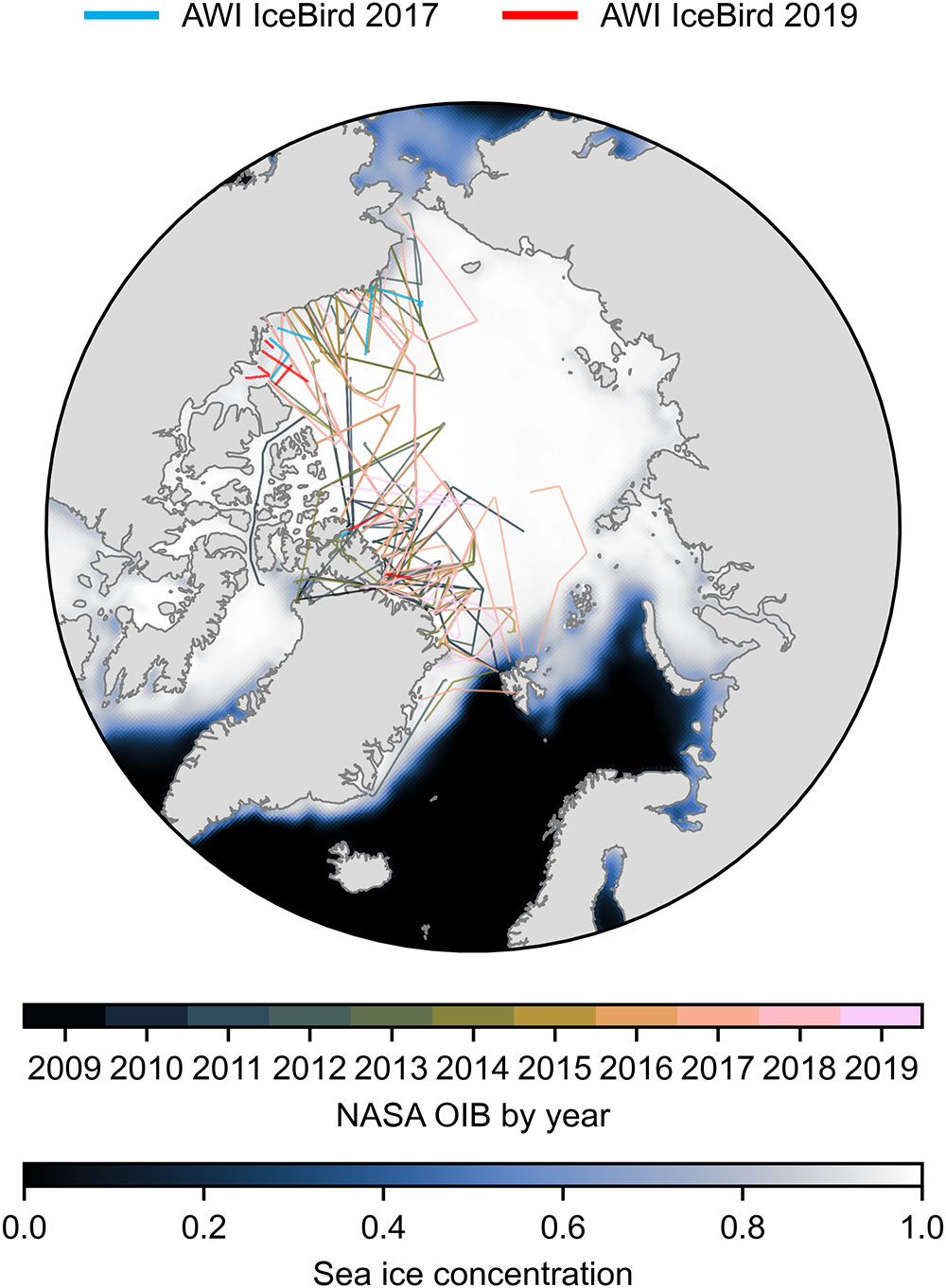
To evaluate SMLG_HS snow depth and sea-ice thickness, we compared them against a total of >100 airborne surveys from the Alfred Wegener Institute’s (AWI) IceBird and NASA OIB campaigns over the western Arctic in late winter 2009–19 (Fig. 1). Summarizing descriptions of the respective datasets are given in the Sections 2.6.1 and 2.6.2. We averaged the airborne measurements over the same model EASE grid when >50 values were present in a grid cell.
Spatial and annual coverage of the 11 AWI IceBird survey flights in 2017 and 2019 (Table 1) and the 99 NASA Operation IceBridge (OIB) survey flights in 2009–19 (Table A1 in Appendix A). The background shows the average March–April monthly sea-ice concentration in 2009–19.
2.6.1. AWI IceBird
The AWI IceBird program carried out 11 survey flights over the western Arctic Ocean in April 2017 and 2019, monitoring the regional sea-ice conditions in very high resolution (Table 1). The nominal measurement spacing along-track is 5–6 m. Snow depth data were derived from an airborne snow radar similar to OIB using the Peakiness retrieval algorithm (Jutila and others, Reference Jutila2021a; Reference Jutila2021b; Reference Jutila2022b). Sea-ice thickness was derived by subtracting snow depth from the total (sea ice + snow) thickness data measured simultaneously with a towed electromagnetic induction sounding instrument (Jutila and others, Reference Jutila, Hendricks, Ricker, von Albedyll, Krumpen and Haas2022a; Reference Jutila, Hendricks, Ricker, von Albedyll and Haas2024a; Reference Jutila, Hendricks, Ricker, von Albedyll and Haas2024b). We distinguished measurements over level ice by using the flag in the data product that implements a sea-ice thickness gradient threshold of 4 cm within an along-track distance of 1 m over continuous sections of at least 100 m long.
Statistics of the 11 AWI IceBird survey flights over the western Arctic Ocean in 2017 and 2019 (Fig. 1) used in this study, where L is the total length of the survey flight,  ${\bar{h}}_{\mathrm{s,level}}$ is the average snow depth on level ice, $\bar{h}_{\mathrm{s,deformed}}$ is the average snow depth on deformed ice, $\bar{h}_{\mathrm{s,all}}$ is the average snow depth of the entire survey flight including all ice types, $\frac{\bar{h}_{\mathrm{s,level}}}{\bar{h}_{\mathrm{s,deformed}}}$ is the fraction of the average snow depth on level ice to the average snow depth on deformed ice, $f_{\mathrm{level}}$ is the level ice fraction of the survey flight, $f_{V_{\mathrm{s,level}}}$ is the fraction of snow volume on level ice, $f_{\mathrm{MYI}}$ is the fraction of multi-year ice (MYI) and $f_{\mathrm{NaN}}$ is the fraction of missing snow depth data
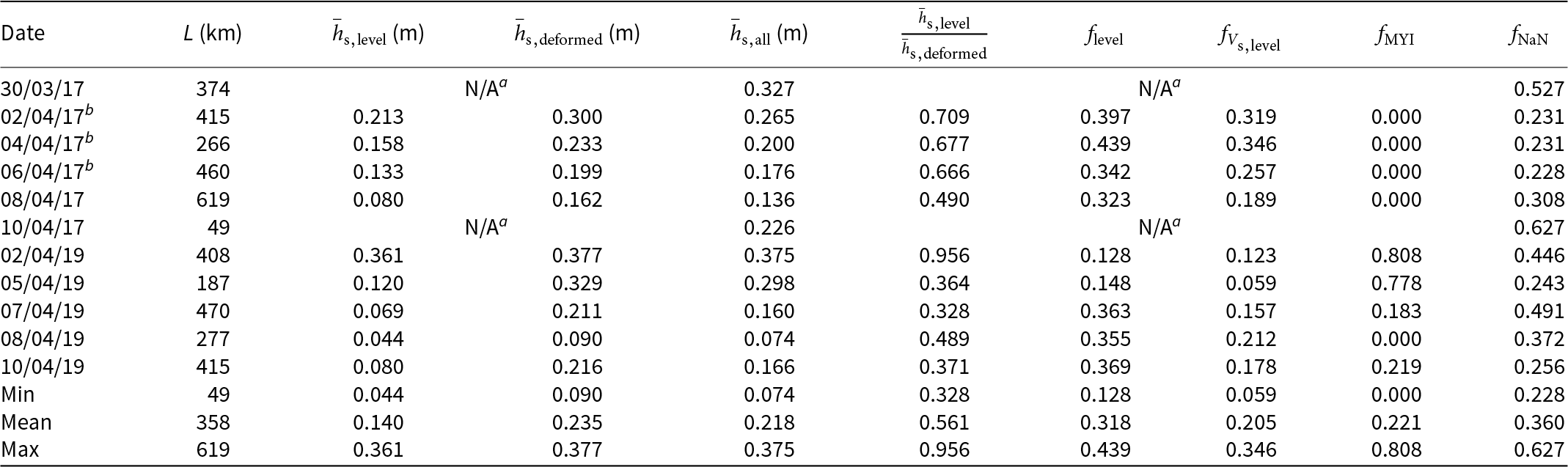
aNot applicable; no sea-ice thickness measurements.
bUsed in the sensitivity experiment (Section 2.7).
2.6.2. NASA OIB
Annual NASA OIB campaigns over the western Arctic Ocean took place in March–April 2009–19 (MacGregor and others, Reference MacGregor2021) and comprise 99 survey flights in total (Table A1 in Appendix A). We used the data products of Kurtz and others (Reference Kurtz, Studinger, Harbeck, DePaul Onana and Yi2015); (Reference Kurtz, Studinger, Harbeck, DePaul Onana and Yi2016) where the snow depth data were derived from airborne snow radars using the retrieval algorithms described in Kurtz and Farrell (Reference Kurtz and Farrell2011); Kurtz and others (Reference Kurtz2013). The data are averaged in the along-track direction to a 40 m length scale. We did not use the OIB sea-ice thickness to evaluate modeled sea-ice thickness, because it is not directly measured but converted from freeboard and snow depth measurements assuming hydrostatic equilibrium. However, we did use it together with surface roughness data included in the product to guide a level ice identification similar to the IceBird data (Jutila and others, Reference Jutila, Hendricks, Ricker, von Albedyll, Krumpen and Haas2022a). To compensate for the increased uncertainty of sea-ice thickness and the approximately 8–10 times coarser along-track resolution compared to the IceBird data, we applied here more strict conditions including a sea-ice thickness gradient threshold of 2 cm m−1 over continuous sections of at least 200 m long as well as ensuring a corresponding surface roughness value of <0.3 m. We determined the numerical values of these conditions through manual iteration and visually inspecting along-track sea-ice transect profiles. Using snow freeboard, snow depth and sea-ice thickness data, we produced figures of snow and sea-ice layer heights with respect to the local sea level (i.e. zero freeboard) in 10 km long along-track segments for five OIB flights from different years and different regions to verify that only truly level ice was identified.
2.7. Sensitivity experiment
Because sub-parcel snow mass redistribution is not considered in the model, we hypothesized that SMLG_HS would overestimate snow depth on level ice and consequently underestimate level ice thickness and overestimate snow-ice thickness. To test our hypothesis, we performed a modeling sensitivity experiment, where we decreased snow depth in SMLG_HS by 10% intervals and compared the simulated snow depth and sea-ice thickness to observations. We conducted in total seven SMLG_HS runs, decreasing the snow depth by 10%, 20%, 30%, 40%, 50%, 60% and 70%, respectively. As observations, we used a subset of IceBird flights in April 2017 that have the highest fractions of level ice and that extend far enough from the vicinity of coastlines, i.e. the edges of the simulation domain (Table 1). The data collected in April 2019 were not included in the experiment due to the smaller fractions of level ice, the presence of deformed multi-year ice and/or the closeness of coastlines. We derived a snow depth fraction that resulted in best fitting of both snow depth and level ice thickness simulations (including snow-ice formation) to the observations. We argue that this snow depth decrease represents the sub-parcel snow mass redistribution sink, because all other snow sinks are accounted for by the model.
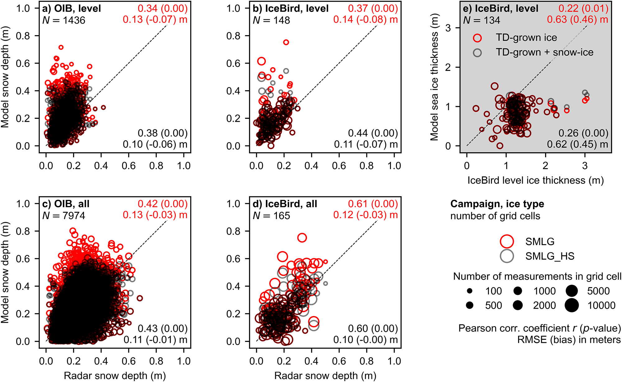
As an independent evaluation, we investigated the snow mass redistribution between level and deformed ice also along the 100+ airborne surveys in 2009–19 by calculating the fraction of snow volume on level ice for each flight:
 \begin{equation}
V_{\mathrm{s,tot}} = V_{\mathrm{s,level}} + V_{\mathrm{s,deformed}} = \bar{h}_{\mathrm{s,level}} \times f_{\mathrm{level}} + \bar{h}_{\mathrm{s,deformed}} \times \left(1 - f_{\mathrm{level}}\right),
\end{equation}
\begin{equation}
V_{\mathrm{s,tot}} = V_{\mathrm{s,level}} + V_{\mathrm{s,deformed}} = \bar{h}_{\mathrm{s,level}} \times f_{\mathrm{level}} + \bar{h}_{\mathrm{s,deformed}} \times \left(1 - f_{\mathrm{level}}\right),
\end{equation}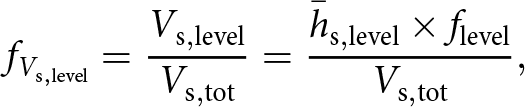 \begin{equation}
f_{V_{\mathrm{s,level}}} = \frac{V_{\mathrm{s,level}}}{V_{\mathrm{s,tot}}} = \frac{\bar{h}_{\mathrm{s,level}} \times f_{\mathrm{level}}}{V_{\mathrm{s,tot}}},
\end{equation}
\begin{equation}
f_{V_{\mathrm{s,level}}} = \frac{V_{\mathrm{s,level}}}{V_{\mathrm{s,tot}}} = \frac{\bar{h}_{\mathrm{s,level}} \times f_{\mathrm{level}}}{V_{\mathrm{s,tot}}},
\end{equation} where  $V_{\mathrm{s,tot}}$ is the total snow volume, $V_{\mathrm{s,level}}$ is the snow volume on level ice, $V_{\mathrm{s,deformed}}$ is the snow volume on deformed ice, $\bar{h}_{\mathrm{s,level}}$ is the average snow depth on level ice, $\bar{h}_{\mathrm{s,deformed}}$ is the average snow depth on deformed ice, $f_{\mathrm{level}}$ is the level ice fraction and $f_{V_{\mathrm{s,level}}}$ is the fraction of snow volume on level ice.
3. Results
In the evaluation exercise, we compared SMLG_HS simulations of snow depth and sea-ice thickness against independent airborne observations from the IceBird and OIB campaigns, and we were able to examine snow depth on level ice separately. The results of the evaluation exercise confirmed our hypothesis. They indicated that SMLG_HS overestimated snow depth over level ice on average by 0.06–0.07 m with a root-mean-square error (RMSE) of 0.10–0.11 m, but with an absolute error up to 0.45 m (Fig. 2a–d and Fig. 3a–b). For comparison, in the SMLG, the maximum absolute error was even higher, 0.60 m. Therefore, SMLG_HS underestimated level ice thickness on average by 0.45 m with an RMSE of 0.62 m, but with an absolute error up to 1.76 m (Fig. 2e–h and Fig. 3e). This result was consistent in all IceBird flights examined in the evaluation exercise.
Panels (a)–(d) show the evaluation of modeled snow depth from SMLG and SMLG_HS against airborne radar-derived snow depth measurements from the AWI IceBird survey flight on 8 April 2017. Red color refers to the original SMLG and black color to the new, coupled SMLG_HS. Panels (e)–(h) show the evaluation of thermodynamically grown (TD-grown) sea ice and snow ice modeled with SMLG_HS against airborne sea-ice thickness measurements over level ice from the same flight. The red square in panels (d) and (h) show the extent of panels (b), (c), (f) and (g). Red color refers to only thermodynamically grown (TD-grown) sea ice, black color indicates the sum of TD-grown sea ice and snow ice, i.e. total sea-ice thickness. In panels (a) and (e), the size of the data point reflects the relative number of airborne measurements in the grid cell. Upper and lower right corners of each panel show the statistics of the corresponding year: Pearson correlation coefficient r, p-value in parenthesis, root-mean-square error (RMSE) and lastly mean bias in parenthesis.
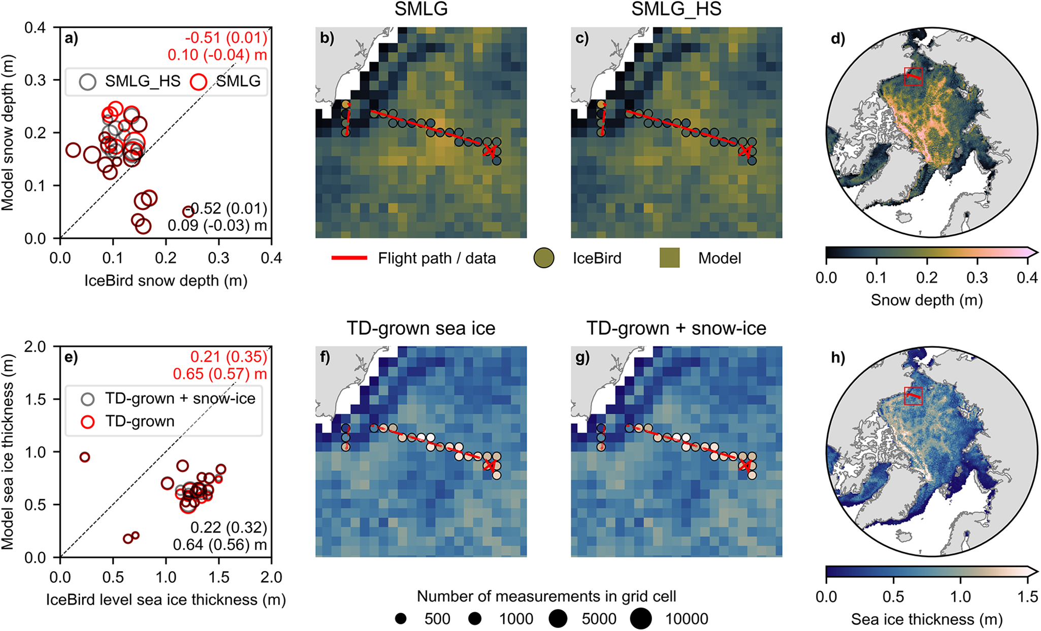
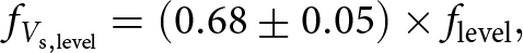
Evaluation of the simulations compared against gridded airborne measurements. Panels (a)–(d) with white background show the modeled snow depth against radar-derived snow depth. The upper panels (a)–(b) show only measurements over level ice and the lower panels (c)–(d) show measurements over all ice types. The left-side panels (a) and (c) show the NASA Operation IceBridge (OIB) flights in 2009–19 and the middle panels (b) and (d) show the AWI IceBird flights in 2017 and 2019. Red color refers to the original SMLG and black color to the new, coupled SMLG_HS. The upper right panel (e) with gray background shows the modeled sea-ice thickness compared against gridded airborne sea-ice thickness measurements over level ice from the AWI IceBird campaigns in 2017 and 2019. Red color refers to only thermodynamically grown (TD-grown) sea ice, black color indicates the sum of TD-grown sea ice and snow ice, i.e. total sea-ice thickness. The size of the data point reflects the relative number of airborne measurements in the grid cell. Upper and lower right corners of each panel show the statistics of the corresponding year: Pearson correlation coefficient r, p-value in parenthesis, root-mean-square error (RMSE) and lastly mean bias in parenthesis.
When we did not distinguish between level and deformed ice and we evaluated SMLG_HS simulations against the total snow depth observations instead (over all ice types), SMLG_HS demonstrated better fit to the snow depth observations from both IceBird and OIB flights (Fig. 2a–d), with reduced RMSEs and biases compared to SMLG (Fig. 3c–d). However, based on a non-parametric Wilcoxon signed-rank test, the differences between the models were not statistically significant. In any case, this indicates that total snow-on-sea-ice amounts given by SMLG_HS are realistic, but they do not account for the sub-grid spatial variations of snow depth (25 km × 25 km). Without considering the sub-grid snow distribution, SMLG_HS overestimated snow depth on level ice resulting in thinner level ice thickness that is more prone to snow-ice formation. The question now becomes: how much snow is removed from the level ice due to snow mass redistribution?
We examined two different approaches to address the question above and to assess the sub-parcel snow mass redistribution: (1) by conducting a modeling sensitivity experiment with a subset of IceBird flights and (2) by performing an analysis of snow volume distribution between level and deformed sea ice based on all IceBird and OIB flight transects. The results of the modeling sensitivity experiment revealed that snow depth on level ice should be reduced by 40% to simulate level ice thickness realistically (Fig. 4) and, at the same time, to maintain snow depth and sea-ice thickness within their respective measurement uncertainties of 0.05 m and 0.12 m for the western Arctic in April 2017. This reduced the mean bias in level sea-ice thickness by 53% from 0.30 m to 0.14 m. The analysis of snow volume distribution along all the OIB and IceBird flight transects in 2009–19 revealed a relationship between the fraction of level ice ( $f_{\mathrm{level}}$) along a sea-ice transect and the fraction of snow volume on level ice ( $f_{V_{\mathrm{s,level}}}$), demonstrating the effect of the sub-parcel snow mass redistribution (Fig. 5). This relationship is linear for fractions of level ice up to 0.5, and it can be given by
 \begin{equation}
f_{V_{\mathrm{s,level}}} = \left(0.68 \pm 0.05\right) \times f_{\mathrm{level}},
\end{equation}
\begin{equation}
f_{V_{\mathrm{s,level}}} = \left(0.68 \pm 0.05\right) \times f_{\mathrm{level}},
\end{equation}where ±0.05 represents the 95% confidence interval of the slope.
Results of the sensitivity experiment showing (a) snow depth over all (level and deformed) ice types, (b) snow depth over level ice only, (c) sea-ice thickness over level ice and (d) location of the three IceBird flights (red lines; Table 1) together with the sea-ice type in April 2017 at the time of the flights. The control simulation with unmodified snow depth (SMLG_HS ctrl) is shown as red circles and the simulation with snow depth reduced by 40% (SMLG_HS 0p6) as black circles. The size of the data point reflects the relative number of airborne measurements in the grid cell. While 38% of the total data are from the level ice, the total number of the grid cells (N = 57) is not reduced. Upper and lower right corners of panels (a)–(c) show the statistics of the datasets: the number above is the Pearson correlation coefficient r with p-value in parenthesis, while below are the root-mean-square error and lastly mean bias in parenthesis. OW stands for open water, FYI for first-year ice, SYI for second-year ice (i.e. sea ice that has survived one melt season) and MYI for multi-year ice (i.e. sea ice that has survived at least two or more melt seasons).
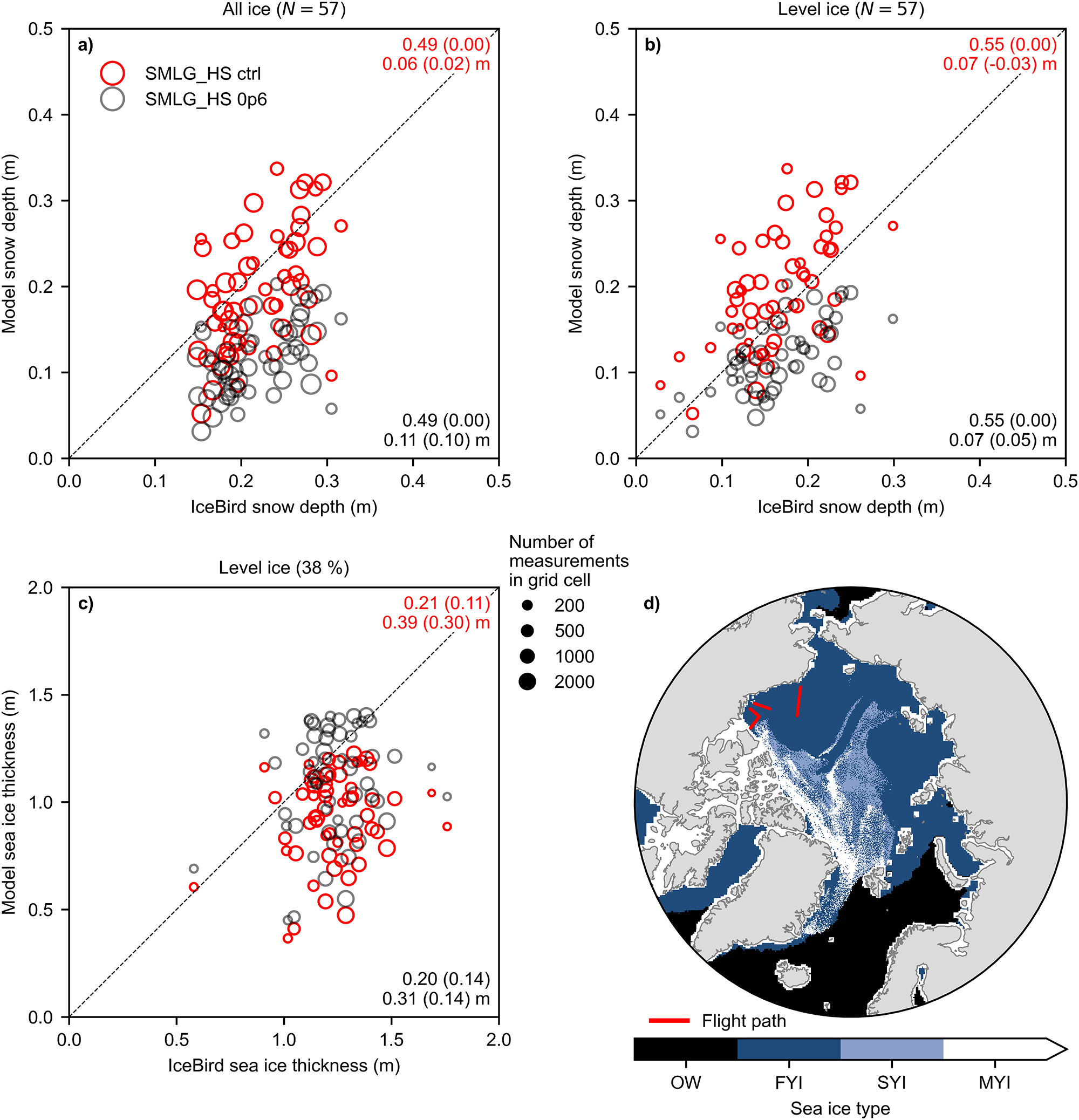
The relationship between the fraction of level ice and the fraction of snow volume on level ice demonstrating the effect of snow mass redistribution (gray hatching). The NASA OIB survey flights are marked with black circles and their linear fit with a black dashed line, whereas the AWI IceBird ones are shown with red crosses and a red dashed line. The solid black line shows the linear fit of all airborne data and the gray shading is its 95% confidence interval. The blue stars show the corresponding end-of-winter values in March–April 2020 from the MOSAiC expedition ground-based transect by Itkin and others Reference Itkin(2023).
4. Discussion
We performed a modeling study to investigate snow sinks on level ice in the western Arctic. Specifically, we examined snow sinks caused by snow and ice interactions, such as snow-ice formation and snow mass redistribution. Snow loss in leads was not considered in this study, because observations from the MOSAiC expedition demonstrated that this is likely an insignificant snow sink in winter, due to quick refreezing of the leads (Clemens-Sewall and others, Reference Clemens-Sewall2023). We coupled SMLG snow depth and density evolution with HIGHTSI thermodynamic sea-ice and snow-ice growth to create SMLG_HS. Being in fact a 1-D model, SMLG_HS should be considered for level ice only. It does not account for dynamic ice thickening, nor for sub-parcel snow mass redistribution processes, i.e. the preference of snow to accumulate over ice deformations (Liston and others, Reference Liston, Polashenski, Rösel, Itkin and King2018). It also assumes that negative freeboard will lead to snow-ice formation. Therefore, it is expected to overestimate snow depth on level ice. Being a very effective insulator, this additional snow decelerates level ice growth, resulting in underestimation of level ice thickness and overestimation of snow-ice thickness. This hypothesis was confirmed when we compared SMLG_HS simulations to airborne observations of snow depth over level ice and level ice thicknesses. SMLG_HS matched the overall snow depth observations from airborne radars better compared to SMLG, with reduced RMSEs and biases. However, based on a statistical test (non-parametric Wilcoxon signed-rank test), the differences between the snow depths in the two models were not statistically significant.
AWI IceBird data are ideal for evaluating SMLG_HS, because they offer simultaneous snow depth and sea-ice thickness observations over hundreds of kilometers of transects in high resolution, with a possibility to examine level and deformed ice conditions separately. However, IceBird campaigns that provide a concrete dataset of both snow depth and sea-ice thickness observations are limited to the western Arctic and in April 2017 and 2019 only. In 2019, IceBird flew over multi-year ice that was heavily deformed, resulting in small fractions of level ice along the flight tracks. The limited level ice observations would impose a risk of unreliable conclusions; therefore, we focused our analysis on flights with the largest level ice fraction in 2017. Moreover, the monitored region was occasionally close to the coast where parcel trajectory data are unavailable, rendering these regions outside the simulation domain and the sensitivity experiment.
The modeling sensitivity experiment showed that reducing snow depth by 40% produced the best agreement between snow depth (on level ice) and level ice thickness in the western Arctic in April 2017 and reduced the mean bias in sea-ice thickness by 53%. The analysis of the snow volume distribution between level and deformed sea ice using observations from the IceBird and OIB transects was in good agreement with the model results when considering their respective limitations. The sensitivity experiment relies on a 1-D thermodynamic model that does not account for lateral conduction of heat, a factor that becomes significant when snow depth varies spatially (Clemens-Sewall and others, Reference Clemens-Sewall, Polashenski, Perovich and Webster2024; Zampieri and others, Reference Zampieri, Clemens-Sewall, Sledd, Hutter and Holland2024). Regarding the airborne approach, it is not possible to account for snow sinks in snow-ice formation. Omitting snow-ice formation, that mostly occurs over level ice, would result in underestimation of the snow mass redistribution.
We argue that the snow depth decrease on level ice represents the sub-parcel snow mass redistribution process; however, this mechanism is not yet fully understood. The deformation rate of a sea-ice floe, together with the atmospheric conditions (e.g. wind, warm intrusions) and the properties of snow cover (density, wetness, sintering level and snow-surface shear strength) are expected to affect the snow redistribution, i.e. the amount of snow removed from the level to deformed ice. Ice and snow conditions are not uniform across the Arctic Ocean, but they vary regionally and temporally. Therefore, a 40% reduction of snow depth on level ice is empirical and more data are needed across the Arctic and the different seasons to study the spatiotemporal variability of snow mass redistribution. In another, yet more local example by Itkin and others Reference Itkin(2023), data from the MOSAiC expedition indicated that 31% of level ice contained only 18% of the snow volume at the end of spring (see the blue stars in Fig. 5). In the Surface Heat Budget of the Arctic Ocean (SHEBA) study in 1997–98, snowdrifts associated with ridges occupied between 3% and 6% of the total study area. The drift sections had mean depths that were on average 30% higher than the surrounding snow (Sturm and others, Reference Sturm, Holmgren and Perovich2002).
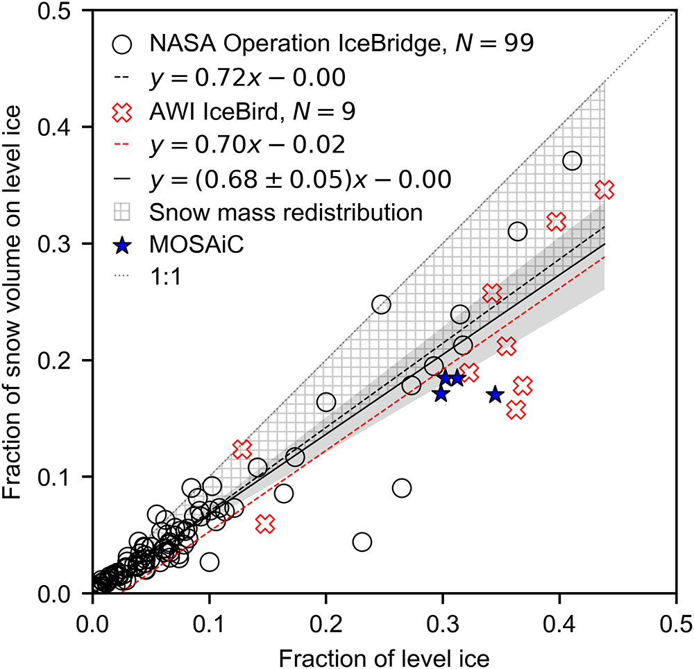
Although the snow depth reduction suggested by the sensitivity experiment cannot be generalized across the entire Arctic and across different years, as an illustrative attempt, we compared snow-ice formation results from the SMLG_HS simulation spanning the years 2007–21, with and without a 40% decrease in snow depth. The 14-year average snow-ice thickness on the day of maximum snow-on-sea-ice volume is shown in Figure 6. Even with a 40% decrease in snow depth, snow ice still has the potential to form and is characterized by strong seasonal and regional variations. However, 40% less snow on level ice would greatly limit snow-ice formation in the central and western Arctic. This process would be primarily restricted to the Atlantic sector of the Arctic, particularly along Greenland’s east coast and north of Svalbard underneath the North Atlantic storm track, where the N-ICE2015 campaign was conducted. Snow-ice formation has also been observed with autonomous sea-ice mass-balance buoys similar to Provost and others Reference Provost(2017) (Text S2 and Fig. S1 in the supplementary material) and in fully coupled climate models (Webster and others, Reference Webster, DuVivier, Holland and Bailey2021) in these regions in the contemporary period. Understanding the importance of sub-parcel snow mass redistribution will guide the development of necessary modeling tools that capture snow sinks properly.
Snow-ice thickness, 14-year average over the day of maximum snow-on-sea-ice volume in 2007–21, from (a) the control run (SMLG_HS ctrl), (b) the run with snow depth reduced by 40% (SMLG_HS 0p6) and (c) the difference between the two simulations (reduced minus control).
5. Conclusions
We showed that a 1-D sea-ice and snow thermodynamic model approach would overestimate snow sink in snow-ice formation. Even though the total snow depth (over both deformed and level ice) matched well with both OIB and IceBird observations, not accounting for snow redistribution from level to deformed ice resulted in overestimation of snow depth over level ice. As expected, this additional snow decelerated thermodynamic ice growth in the model, resulting in thinner level ice that is more prone to snow-ice formation. Based on the evaluation of our simulations against IceBird data in April 2017, fitting both snow on level ice and level ice thickness simulations to the IceBird observations, snow depth in SMLG_HS should be reduced by 40%. We argue that in our 2017 case study in the western Arctic, 40% reduction in snow depth over level ice represented the sub-parcel snow mass redistribution process. Based on the analysis of >100 airborne survey flights spanning a full decade, the fraction of snow volume on level ice in spring is linearly related to the level ice fraction, and it is given by  $f_{V_{\mathrm{s,level}}} = \left(0.68 \pm 0.05\right) \times f_{\mathrm{level}}$. This linear relationship indicates that the amount of snow remaining on level sea ice in the end of winter is proportional to the amount of ice deformation.
When snow models do not account for snow sinks caused by snow and sea-ice interactions, such as snow-ice formation or sub-parcel snow mass redistribution processes, they overestimate snow depth on level ice. Uneven snow-on-sea-ice load within a sub-grid area will result in biases in altimetry retrievals of sea-ice thickness by overestimating level ice and underestimating deformed ice thickness. Regarding sea-ice modeling applications, spatial variability in snow depth will impact sea-ice thermodynamic growth in winter, affecting both vertical and horizontal heat fluxes, and will influence melt pond formation in summer (Thielke and others, Reference Thielke2023). Therefore, snow-on-sea-ice reconstructions should be used with caution depending on the application requirements. This study emphasizes the need to account for sub-grid scale heterogeneity in snow and sea-ice interactions to improve the representation of snow in remote sensing and model studies. It also highlights the crucial need for additional independent but simultaneous observations of snow depth and sea-ice thickness, together with information on snow properties, to understand the mechanism behind snow mass changes due to coupled physical processes.
Supplementary material
The supplementary material for this article can be found at https://doi.org/10.1017/jog.2025.34.
Acknowledgements
IM was supported by the ESA grant CCI+ 4000126449/19/I-NB. IM and AJ were supported by the Research Council of Finland grant 341550. GEL was supported by the United States National Science Foundation grant 1820927. AP was supported by the European Union’s Horizon 2020 research and innovation program under grant 101003472. MAW conducted this work under the National Science Foundation Project 2325430. The authors are grateful to Bin Cheng for providing the software code for the model HIGHTSI and to Polona Itkin for sharing the MOSAiC ground-based transect data. Autonomous sea-ice measurements (temperature profile and heating cycle data) from 2012 to 2020 were obtained from https://www.meereisportal.de (grant: REKLIM-2013-04). The scientific color maps (Crameri, Reference Crameri2023) are used in this study to prevent visual distortion of the data and exclusion of readers with color-vision deficiencies (Crameri and others, Reference Crameri, Shephard and Heron2020).
Author contributions
Conceptualization: IM. Data curation: IM, AJ, GEL, AP. Formal analysis: IM, AJ, GEL. Funding acquisition: IM. Investigation: IM, AJ. Methodology: IM, GEL. Project administration: IM. Resources: IM. Software: AJ, GEL. Supervision: IM. Validation: IM, AJ, GEL. Visualization: AJ. Writing—original draft: IM. Writing—review & editing: IM, AJ, GEL, AP, MAW. Author contributions follow the Contributor Role Taxonomy (CRediT) (Brand and others, Reference Brand, Allen, Altman, Hlava and Scott2015; National Information Standards Organization (NISO), 2022).
Data availability statement
Sea-ice concentration data are available at DiGirolamo and others Reference DiGirolamo, Parkinson, Cavalieri, Gloersen and Zwally(2022). Sea-ice motion vectors are available at Tschudi and others Reference Tschudi, Meier, Stewart, Fowler and Maslanik(2019). Atmospheric forcing data are available at Global Modeling And Assimilation Office (GMAO) (2015a); (2015b). Daily ocean heat flux data (opa0/daily_r1x1) were downloaded from ECMWF via the ECMWF ECGATE Class Service (ECS) computing facility using Teleport SSH and a personal ECMWF user account. Airborne data are available at Jutila and others (Reference Jutila2021a); (Reference Jutila2021b); (Reference Jutila, Hendricks, Ricker, von Albedyll and Haas2024a); (Reference Jutila, Hendricks, Ricker, von Albedyll and Haas2024b) for AWI IceBird and at Kurtz and others (Reference Kurtz, Studinger, Harbeck, DePaul Onana and Yi2015); (Reference Kurtz, Studinger, Harbeck, DePaul Onana and Yi2016) for NASA OIB. Data for SIMBA buoys are available at Preußer and others Reference Preußer, Nicolaus and Hoppmann(2025).
Competing interests
The authors have no competing interests to declare.
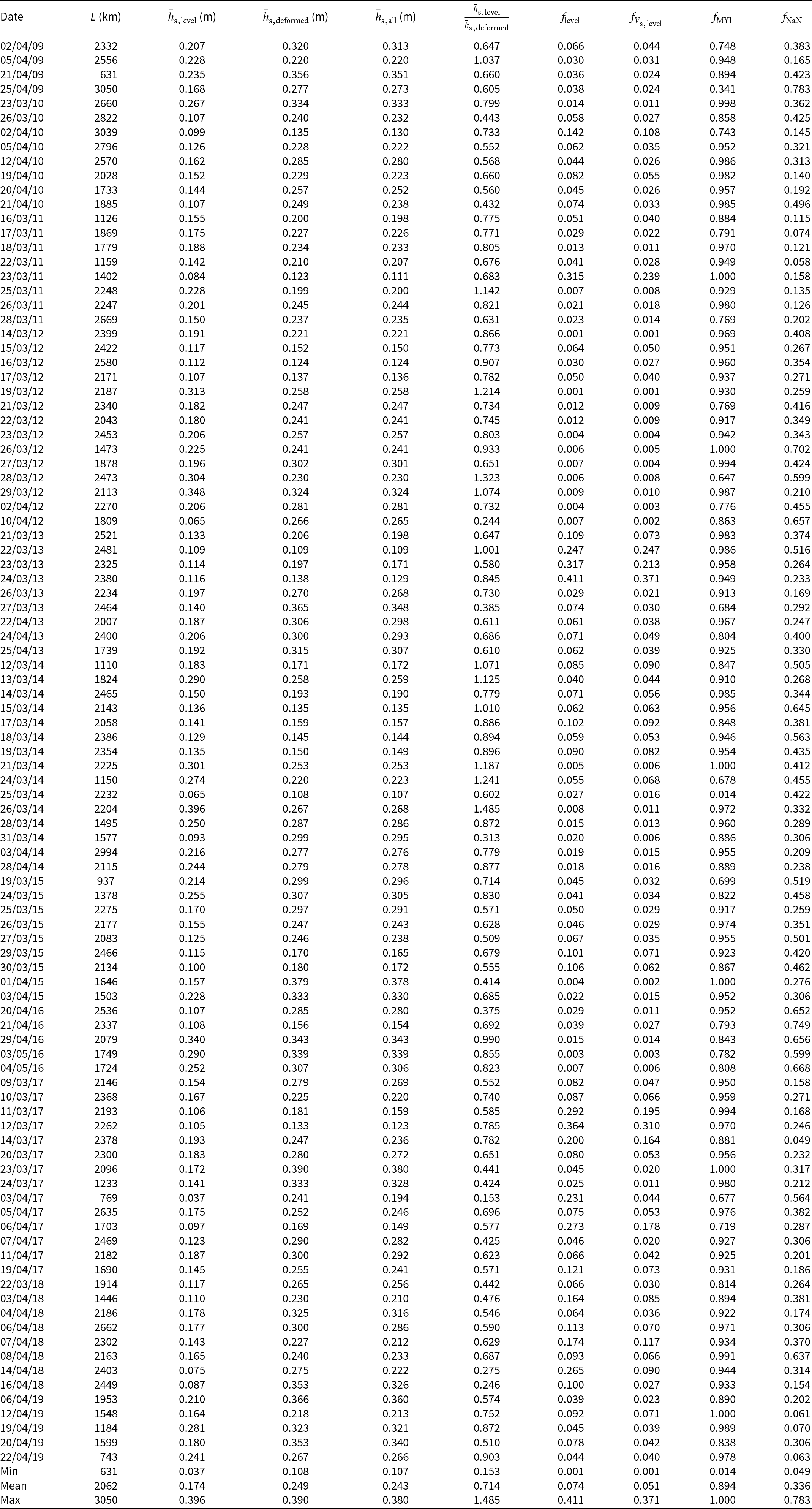
Appendix A. NASA OIB survey statistics
Statistics of the 99 NASA Operation IceBridge survey flights over the western Arctic Ocean in 2009–19 (Fig. 1) used in this study, where L is the total length of the survey flight,  $\bar{h}_{\mathrm{s,level}}$ is the average snow depth on level ice, $\bar{h}_{\mathrm{s,deformed}}$ is the average snow depth on deformed ice, $\bar{h}_{\mathrm{s,all}}$ is the average snow depth of the entire survey flight including all ice types, $\frac{\bar{h}_{\mathrm{s,level}}}{\bar{h}_{\mathrm{s,deformed}}}$ is the fraction of the average snow depth on level ice to the average snow depth on deformed ice, $f_{\mathrm{level}}$ is the level ice fraction of the survey flight, $f_{V_{\mathrm{s,level}}}$ is the fraction of snow volume on level ice, $f_{\mathrm{MYI}}$ is the fraction of multi-year ice (MYI) and $f_{\mathrm{NaN}}$ is the fraction of missing snow depth data


 Open access