
 R−L
R−L R−L
R−L








1. Introduction
Every massive galaxy is thought to host a super-massive black hole (SMBH) at its core, with these objects believed to play an important role in galaxy evolution (Kormendy & Ho Reference Kormendy and Ho2013). Despite their ubiquity, these objects remain poorly understood, with the exact mechanisms of their formation and growth within their host galaxies remaining as open questions (e.g. Volonteri et al. Reference Volonteri, Habouzit and Colpi2021). Measuring the mass of these SMBHs over cosmic time is then of great interest, as it offers us insight into the history and evolution of these important objects.
As dark and compact objects, our ability to observe SMBHs by electromagnetic means relies on observations of their environment, and that ability drops rapidly with distance. This obstacle would frustrate our attempts to observe them into the cosmic past were it not for Active Galactic Nuclei (AGN), extremely luminous SMBHs with bright accretion disks that can easily outshine their entire host galaxy. Under the standard model (Urry & Padovani Reference Urry and Padovani1995), these AGN consist of a central black hole/accretion disk ‘engine’ and a complex surrounding structure, including the fast orbiting material in the broad line region (BLR). As the luminosity, kinematics and structure of the AGN are all powered by the driving gravitational force of the central black hole, many of the AGN’s physical properties offer means of inferring the mass of the black hole.
AGN in the local universe can have their masses constrained by the kinematics of their surrounding stars, either directly tracking orbits (e.g. Schödel et al. Reference Schödel2002) or the bulk stellar velocity dispersion (i.e. the ‘ $M-\sigma$
relation’ Ferrarese & Merritt Reference Ferrarese and Merritt2000; Gebhardt et al. Reference Gebhardt2000), but such techniques become challenging at larger distances where entire galaxies appear as AGN-dominated point sources. The previous decade has also seen considerable progress in imaging two of the nearest SMBHs with interferometry at millimetre wavelengths (e.g. Akiyama et al. Reference Akiyama2019), and in using Very Large Telescope interferometry to potentially access finer angular resolutions (Gravity+ Collaboration et al. 2022). At higher redshifts, the limits on angular resolutions can also be surpassed with reverberation mapping (RM), a technique in which temporal coverage of variability can substitute for a lack of spatial information (Blandford & McKee Reference Blandford and McKee1982; Peterson Reference Peterson1993).
$M-\sigma$
relation’ Ferrarese & Merritt Reference Ferrarese and Merritt2000; Gebhardt et al. Reference Gebhardt2000), but such techniques become challenging at larger distances where entire galaxies appear as AGN-dominated point sources. The previous decade has also seen considerable progress in imaging two of the nearest SMBHs with interferometry at millimetre wavelengths (e.g. Akiyama et al. Reference Akiyama2019), and in using Very Large Telescope interferometry to potentially access finer angular resolutions (Gravity+ Collaboration et al. 2022). At higher redshifts, the limits on angular resolutions can also be surpassed with reverberation mapping (RM), a technique in which temporal coverage of variability can substitute for a lack of spatial information (Blandford & McKee Reference Blandford and McKee1982; Peterson Reference Peterson1993).
Conceptually, reverberation mapping is straightforward: stochastic variations in the brightness of the AGN’s central engine drive variations in the brightness of gas in the surrounding broad-line region, but do so with a time delay associated with light travel time between the central engine and the BLR. Where we can distinguish signals from different regions, we can characterise the scale of this time delay and so infer the physical scale of the AGN (see Figure 1 for a sketch of this process with simplified geometry). Knowledge of this geometric scale, coupled with a measure of the velocity and assumptions about kinematics, provides a means of constraining the mass of the SMBH. As such, reverberation mapping of AGN has become the primary means of constraining SMBH masses at any appreciable redshift, dominating over all other methods beyond $z\approx0.1$
(Cackett et al. Reference Cackett, Bentz and Kara2021).
$z\approx0.1$
(Cackett et al. Reference Cackett, Bentz and Kara2021).
Simplified model of reverberation mapping, showing the different light travel paths for direct and re-processed light. In its simplest ‘single lag’ form, BLR RM relies on the assumption that the accretion disk and BLR are homogeneous, that the accretion disk be reasonably small compared to their angular separation, and the kinematics of the BLR along the line of site be reasonably well characterised by a single representative radius (Shakura & Sunyaev Reference Shakura and Sunyaev1973; Cackett et al. Reference Cackett, Bentz and Kara2021). Additional geometric complexity is characterised by the virial factor $\langle {f}\rangle$
defined in equation (1).
$\langle {f}\rangle$
defined in equation (1).

Figure 1. Long description
A diagram of reverberation mapping, showing the different light travel paths for direct and reprocessed light. The central point source represents the accretion disk emitting continuum light. This light travels outward and interacts with the broad line region (BLR), causing reprocessed BLR emission. An observer detects the continuum signal and the response signal, with a noticeable signal lag between them. The diagram highlights the light travel distance R and the interaction between the continuum light and the BLR.
For most of the history of reverberation mapping, data have been limited to studies of a hand-full of AGN at a time, predominantly at low redshift (e.g. Peterson et al. Reference Peterson1999, Reference Peterson2005; Denney et al. Reference Denney2006), limited by the difficulty of continuous photometric and spectroscopic observations over the required time scales. This has changed with the advent of the first generation of ‘industrial scale surveys’, in which reverberation mapping is performed on hundreds of AGN at redshifts probing into the deep cosmological past. Over the last decade, surveys like the Australian Dark Energy Survey (OzDES; King Reference King2015) and the Sloan Digital Sky Survey (SDSS; Shen et al. Reference Shen2015) have made regular photometric and spectroscopic measurements of well over $1\,000$
AGN in the redshift range
$1\,000$
AGN in the redshift range $0 \lt z\lesssim4.5$
, dramatically increasing the number of distant AGN observations with optical RM data to a statistically significant sample, and pushing our constraints on SMBH masses well into the high redshift domain.
$0 \lt z\lesssim4.5$
, dramatically increasing the number of distant AGN observations with optical RM data to a statistically significant sample, and pushing our constraints on SMBH masses well into the high redshift domain.
Reverberation mapping is observationally expensive, requiring many epochs of observation. However, black hole masses can be derived with single epoch spectral observations through an empirically observed power-law relationship between luminosity and reverberation timescale (or lag) for each line, the so-called ‘ $R-L$
Relationship’. The parameters of these relationships are calibrated using RM and they are reasonably well defined at low redshift, but the paucity of measurements of more distant AGN means that there has been difficulty constraining
$R-L$
Relationship’. The parameters of these relationships are calibrated using RM and they are reasonably well defined at low redshift, but the paucity of measurements of more distant AGN means that there has been difficulty constraining $R-L$
relations for high redshift AGN. One of the aims of OzDES has been to fill that observational gap. Here we present the complete OzDES RM sample and also make a comprehensive collation and comparison of contemporary reverberation mapping surveys, and create a catalogue of the SMBH masses derived from reverberation mapping.
$R-L$
relations for high redshift AGN. One of the aims of OzDES has been to fill that observational gap. Here we present the complete OzDES RM sample and also make a comprehensive collation and comparison of contemporary reverberation mapping surveys, and create a catalogue of the SMBH masses derived from reverberation mapping.
The paper is organised as follows. We discuss the physical principles of reverberation mapping in Section 2, including methods and limitations. In Section 3 we introduce the OzDES and external datasets used in this paper, and then in Section 4 we introduce the methodology used by OzDES, including lag measurement procedures and quality cuts, used to define this dataset. We then present the full suite of recovered lags, SMBH masses and other results from the OzDES RM program in Section 5. In Section 6.1, we compare the $R-L$
relationship constraints of OzDES against those of SDSS and a wide range of other surveys for the H
$R-L$
relationship constraints of OzDES against those of SDSS and a wide range of other surveys for the H $\beta$
, MgII and CIV lines, identifying where they agree or are in tension in the
$\beta$
, MgII and CIV lines, identifying where they agree or are in tension in the $R-L$
plane, and use a combined dataset to tightly constrain the
$R-L$
plane, and use a combined dataset to tightly constrain the $R-L$
slope, offset and scatter for all three lines for samples similar to OzDES and SDSS. In Section 6.2, we confirm an absence of systematic biases from emission-line width or accretion rate for these
$R-L$
slope, offset and scatter for all three lines for samples similar to OzDES and SDSS. In Section 6.2, we confirm an absence of systematic biases from emission-line width or accretion rate for these $R-L$
fits. In Section 7, we derive a bolometric
$R-L$
fits. In Section 7, we derive a bolometric $R-L$
relation and use the different lag predictions for H
$R-L$
relation and use the different lag predictions for H $\beta$
, MgII and CIV as a probe of the relative scales of their emission regions. We then apply the updated
$\beta$
, MgII and CIV as a probe of the relative scales of their emission regions. We then apply the updated $R-L$
relationships in Section 8 to derive single-epoch SMBH masses for 246 AGN, and finally discuss the results of this paper, examining possible implications about the evolution of SMBH populations via our single epoch mass estimates, in Section 9.
$R-L$
relationships in Section 8 to derive single-epoch SMBH masses for 246 AGN, and finally discuss the results of this paper, examining possible implications about the evolution of SMBH populations via our single epoch mass estimates, in Section 9.
2. Technique and limitations
2.1. Reverberation mapping
The core of AGN reverberation mapping is based on arguments of the virialised orbit of the broad line region about the black hole, with the SMBH mass being correlated with the estimated radius of the BLR, $R_\mathrm{BLR}$
, and its velocity dispersion
$R_\mathrm{BLR}$
, and its velocity dispersion $\langle{\sigma_v^2}\rangle$
as in equation (1). The complexities of the BLR’s unresolved geometry are captured in the broad uncertainties of the dimensionless ‘virial factor’, f:Footnote
a
$\langle{\sigma_v^2}\rangle$
as in equation (1). The complexities of the BLR’s unresolved geometry are captured in the broad uncertainties of the dimensionless ‘virial factor’, f:Footnote
a
 \begin{equation} M_\textrm{BH} = f\frac{ R_\textrm{BLR} \langle{\sigma_v^2}\rangle }{G}. \end{equation}
Though conceptually simple, each term in the numerator of equation (1) is non-trivial to measure for any given source. One hurdle is that the kinematics at play are dependent on the shape and dynamics of the BLR, the nature of which is as yet unresolved (Pancoast et al. Reference Pancoast, Brewer and Treu2014a,b). This uncertainty is quantified by calibrating the population average virial factor, $\langle{f}\rangle$
from population analysis of nearby AGN, the masses of which are estimated through use of the
$\langle{f}\rangle$
from population analysis of nearby AGN, the masses of which are estimated through use of the $M-\sigma$
relation (Woo et al. Reference Woo, Yoon, Park, Park and Kim2015; Grier et al. Reference Grier2013a), or more recently through dynamical modelling via velocity resolved reverberation mapping (Villafaña et al. Reference Villafaña2023; Shen et al. Reference Shen2024). The f is only loosely constrained for any individual source, as there is an inherent scatter of
$M-\sigma$
relation (Woo et al. Reference Woo, Yoon, Park, Park and Kim2015; Grier et al. Reference Grier2013a), or more recently through dynamical modelling via velocity resolved reverberation mapping (Villafaña et al. Reference Villafaña2023; Shen et al. Reference Shen2024). The f is only loosely constrained for any individual source, as there is an inherent scatter of $\approx0.3$
–
$\approx0.3$
– $0.4$
dex about
$0.4$
dex about $\langle {f}\rangle$
, and this dominates the uncertainty in BLR RM derived masses (Woo et al. Reference Woo, Yoon, Park, Park and Kim2015; Shen et al. Reference Shen2023).
$\langle {f}\rangle$
, and this dominates the uncertainty in BLR RM derived masses (Woo et al. Reference Woo, Yoon, Park, Park and Kim2015; Shen et al. Reference Shen2023).
Measurements of $\langle{\sigma_v^2} \rangle$
are made from the spectroscopic broadening of the reverberating emission lines, either by their full-width half-maximum (FWHM), or their dispersion (i.e. the second moment of the line profile about its peak), with different virial factors being tuned for each (see Section 3.3 for examples of RM papers using either technique).
$\langle{\sigma_v^2} \rangle$
are made from the spectroscopic broadening of the reverberating emission lines, either by their full-width half-maximum (FWHM), or their dispersion (i.e. the second moment of the line profile about its peak), with different virial factors being tuned for each (see Section 3.3 for examples of RM papers using either technique).
High redshift AGN are beyond the distances at which we have been able to angularly resolve $R_{\mathrm{BLR}}$
, and so BLR RM instead uses the timescale at which light propagates through the AGN geometry to measure this size by proxy (see Figure 1). Variations in broad band photometric luminosity are dominated by the light emanating directly from the accretion disk ‘engine’, with these variations being echoed in the driven response in the emission lines of the BLR after some delay,
$R_{\mathrm{BLR}}$
, and so BLR RM instead uses the timescale at which light propagates through the AGN geometry to measure this size by proxy (see Figure 1). Variations in broad band photometric luminosity are dominated by the light emanating directly from the accretion disk ‘engine’, with these variations being echoed in the driven response in the emission lines of the BLR after some delay, $\Delta t$
, typically of order days to months. The BLR spectrum exhibits atomic recombination lines that can be easily distinguished from the broad AGN continuum emission, allowing us to identify this echo through spectroscopic observations even where our photometric observations are dominated by light from the accretion disk. With sufficiently tight cadence of photometric and spectroscopic observations, the delay (or lag) between driving continuum and driven emission line response,
$\Delta t$
, typically of order days to months. The BLR spectrum exhibits atomic recombination lines that can be easily distinguished from the broad AGN continuum emission, allowing us to identify this echo through spectroscopic observations even where our photometric observations are dominated by light from the accretion disk. With sufficiently tight cadence of photometric and spectroscopic observations, the delay (or lag) between driving continuum and driven emission line response, $\Delta t$
can be observed, allowing temporal resolution of observations to substitute for the lack of spatial resolution:
$\Delta t$
can be observed, allowing temporal resolution of observations to substitute for the lack of spatial resolution:
 \begin{equation} R_{\mathrm{BLR}} = c \Delta t .\end{equation}
To perform reverberation mapping, a source must provide a clearly identifiable reverberating emission line from the BLR. At cosmological scales, the emission from different emission lines redshift in and out of typical spectroscopic wavelength ranges, and so different atomic emission lines are visible at near, moderate, and high redshift ranges.
For the nearest AGN ( $z\lesssim0.6$
), optical RM is performed with H
$z\lesssim0.6$
), optical RM is performed with H $\alpha$
at
$\alpha$
at $6\,562\,\unicode{x00C5}$
and H
$6\,562\,\unicode{x00C5}$
and H $\beta$
at
$\beta$
at $4\,861 \unicode{x00C5}$
(e.g. Bentz et al. Reference Bentz2014). Beyond measuring the mean lag, some studies have even gone as far as using high signal to noise (SNR) measurements of hydrogen recombination lines to constrain the BLR structure and kinematics in further detail. In this ‘velocity resolved reverberation mapping’ (e.g. Denney et al. Reference Denney2009; Grier et al. Reference Grier2013b), the reverberating line is treated as being affected by varying degrees of Doppler broadening from different velocities at different radii within the BLR, resulting in different parts of the line profile reverberating at different times.
$4\,861 \unicode{x00C5}$
(e.g. Bentz et al. Reference Bentz2014). Beyond measuring the mean lag, some studies have even gone as far as using high signal to noise (SNR) measurements of hydrogen recombination lines to constrain the BLR structure and kinematics in further detail. In this ‘velocity resolved reverberation mapping’ (e.g. Denney et al. Reference Denney2009; Grier et al. Reference Grier2013b), the reverberating line is treated as being affected by varying degrees of Doppler broadening from different velocities at different radii within the BLR, resulting in different parts of the line profile reverberating at different times.
At higher redshifts ( $0.6\lesssim z\lesssim1.8$
), optical RM is performed with the MgII line at
$0.6\lesssim z\lesssim1.8$
), optical RM is performed with the MgII line at $2\,798\,\unicode{x00C5}$
(e.g. Metzroth et al. Reference Metzroth, Onken and Peterson2006). optical RM masses derived from MgII are complicated by iron contamination from the adjacent FeII emission lines, which can distort estimates of the line width unless accounted for (discussed in detail in Section 4).
$2\,798\,\unicode{x00C5}$
(e.g. Metzroth et al. Reference Metzroth, Onken and Peterson2006). optical RM masses derived from MgII are complicated by iron contamination from the adjacent FeII emission lines, which can distort estimates of the line width unless accounted for (discussed in detail in Section 4).
At high redshift ( $z\gtrsim 1.8$
), optical RM is performed with the CIV line at
$z\gtrsim 1.8$
), optical RM is performed with the CIV line at $1\,549\,\unicode{x00C5}$
. CIV lag measurements have also been made by observing this line in the observer-frame UV range for low redshift and low luminosity sources (e.g. Rosa et al. Reference Rosa2015; Peterson et al. Reference Peterson2005; Metzroth et al. Reference Metzroth, Onken and Peterson2006).
$1\,549\,\unicode{x00C5}$
. CIV lag measurements have also been made by observing this line in the observer-frame UV range for low redshift and low luminosity sources (e.g. Rosa et al. Reference Rosa2015; Peterson et al. Reference Peterson2005; Metzroth et al. Reference Metzroth, Onken and Peterson2006).
The $R-L$
relationship (Kaspi et al. Reference Kaspi2000), an empirically observed correlation between the luminosity of an AGN and its physical scale as recovered from RM, is parameterised as a power-law expressed as:
$R-L$
relationship (Kaspi et al. Reference Kaspi2000), an empirically observed correlation between the luminosity of an AGN and its physical scale as recovered from RM, is parameterised as a power-law expressed as:
 \begin{equation}a ,\end{equation}
where $\Delta t$
is the rest-frame lag and
$\Delta t$
is the rest-frame lag and $\lambda L_{\lambda}$
is the monochromatic luminosity of the AGN at a line-specific wavelength: typically
$\lambda L_{\lambda}$
is the monochromatic luminosity of the AGN at a line-specific wavelength: typically $5\,100\,\unicode{x00C5}$
for H
$5\,100\,\unicode{x00C5}$
for H $\beta$
,
$\beta$
, $3\,000\,\unicode{x00C5}$
for MgII, and
$3\,000\,\unicode{x00C5}$
for MgII, and $1\,350\,\unicode{x00C5}$
for CIV. Though the
$1\,350\,\unicode{x00C5}$
for CIV. Though the $R-L$
relationship for H
$R-L$
relationship for H $\beta$
is well constrained and found to have small scatter (
$\beta$
is well constrained and found to have small scatter ( $\approx 0.1$
–
$\approx 0.1$
– $0.2$
dex; Bentz et al. Reference Bentz2013), recent surveys have suggested this scatter may be higher (e.g. Du et al. Reference Du2016, Reference Du2018). The historical
$0.2$
dex; Bentz et al. Reference Bentz2013), recent surveys have suggested this scatter may be higher (e.g. Du et al. Reference Du2016, Reference Du2018). The historical $R-L$
relations for MgII and CIV are found to have higher scatter than H
$R-L$
relations for MgII and CIV are found to have higher scatter than H $\beta$
(Zajaček et al. Reference Zajaček2020; Kaspi et al. Reference Kaspi2007).
$\beta$
(Zajaček et al. Reference Zajaček2020; Kaspi et al. Reference Kaspi2007).
The strong dependence of AGN lags on luminosity has given rise to the technique of stacking (Fine et al. Reference Fine2012, Reference Fine2013; Li et al. Reference Li2017), in which sources of poor signal to noise but similar luminosity have their lag measurements combined. Through stacking, lag measurements can be made up in aggregate over many sources that would otherwise give poorly constrained results, such as done for the OzDES data in (Malik et al. Reference Malik2024).
There have been attempts to explain the diversity of lags through more expressive $R-L$
relationships, reducing the intrinsic scatter by adding predictive variables or dividing the AGN population into sub-groups based on the spectral properties (e.g. Mejía-Restrepo et al. Reference Mejía-Restrepo, Trakhtenbrot, Lira and Netzer2018, Reference Mejía-Restrepo, Trakhtenbrot, Lira, Netzer and Capellupo2016). There is, for example, some evidence that lags are lower for highly accreting sources, above some critical threshold (Du et al. Reference Du2016, Reference Du2018). This is described by the dimensionless accretion rate,
$R-L$
relationships, reducing the intrinsic scatter by adding predictive variables or dividing the AGN population into sub-groups based on the spectral properties (e.g. Mejía-Restrepo et al. Reference Mejía-Restrepo, Trakhtenbrot, Lira and Netzer2018, Reference Mejía-Restrepo, Trakhtenbrot, Lira, Netzer and Capellupo2016). There is, for example, some evidence that lags are lower for highly accreting sources, above some critical threshold (Du et al. Reference Du2016, Reference Du2018). This is described by the dimensionless accretion rate, $\dot{M}$
, given by equation (4), based on the thin-disk model of Shakura & Sunyaev (Reference Shakura and Sunyaev1973).
$\dot{M}$
, given by equation (4), based on the thin-disk model of Shakura & Sunyaev (Reference Shakura and Sunyaev1973).
 \begin{equation} \dot{M} = 20.1 \left( \frac{L_{5\,100\,\unicode{x00C5}} / 10^{44} \mathrm{erg/s}}{\cos(i)} \right)^\frac{3}{2} \left( \frac{M}{10^7\,\mathrm{M_{\odot}}}\right)^{-2}. \end{equation}
Here, $\cos(i)$
is the cosine of the inclination of the AGN, taken to be
$\cos(i)$
is the cosine of the inclination of the AGN, taken to be $0.75$
as an average value for the quasar inclinations in which the BLR and accretion disk are both visible (Seyfert – 1 type AGN), while
$0.75$
as an average value for the quasar inclinations in which the BLR and accretion disk are both visible (Seyfert – 1 type AGN), while $L_{5\,100\,\unicode{x00C5}}$
is the bolometric luminosity at
$L_{5\,100\,\unicode{x00C5}}$
is the bolometric luminosity at $5\,100\,\unicode{x00C5}$
in units of
$5\,100\,\unicode{x00C5}$
in units of $10^{44}\,\mathrm{erg/s}$
and M is the RM-derived SMBH mass in units of
$10^{44}\,\mathrm{erg/s}$
and M is the RM-derived SMBH mass in units of $10^7$
solar masses. The Super-Eddington Accreting Mass Black Hole (SEAMBH) collaboration use
$10^7$
solar masses. The Super-Eddington Accreting Mass Black Hole (SEAMBH) collaboration use $\dot{M}\gt3$
as a benchmark for the separation between low accretion ‘sub-Eddington’ sources and the highly accreting ‘super-Eddington’ sources (Du et al. Reference Du2015, Reference Du2016).
$\dot{M}\gt3$
as a benchmark for the separation between low accretion ‘sub-Eddington’ sources and the highly accreting ‘super-Eddington’ sources (Du et al. Reference Du2015, Reference Du2016).
2.2. The aliasing problem
Though the uncertainties in $M_\mathrm{BH}$
within a single source are dominated by the
$M_\mathrm{BH}$
within a single source are dominated by the $0.3$
–
$0.3$
– $0.4 $
dex population variability in f, lag-recovery presents significant issues with bias and contamination of mass estimates. Cosmological time-dilation means that distant AGN have longer timescales of variability (Lewis & Brewer Reference Lewis and Brewer2023), meaning that RM requires such sources to be observed over a baseline of multiple years to adequately capture variations in their light curves. For the ground-based observations of most distant RM-campaigns, such multi-year observations are necessarily impacted by a seasonal windowing function that imposes
$0.4 $
dex population variability in f, lag-recovery presents significant issues with bias and contamination of mass estimates. Cosmological time-dilation means that distant AGN have longer timescales of variability (Lewis & Brewer Reference Lewis and Brewer2023), meaning that RM requires such sources to be observed over a baseline of multiple years to adequately capture variations in their light curves. For the ground-based observations of most distant RM-campaigns, such multi-year observations are necessarily impacted by a seasonal windowing function that imposes $\sim$
6-month gaps in observations. These seasonal gaps give rise to the problem of ‘aliasing’ (see Figure 2), which can yield spurious lag recoveries at
$\sim$
6-month gaps in observations. These seasonal gaps give rise to the problem of ‘aliasing’ (see Figure 2), which can yield spurious lag recoveries at $n+1/2$
yearly gaps (180 d, 420 d, etc.; Penton et al. Reference Penton2021; Malik et al. Reference Malik2022).
$n+1/2$
yearly gaps (180 d, 420 d, etc.; Penton et al. Reference Penton2021; Malik et al. Reference Malik2022).
Qualitative demonstration of the source of the aliasing problem for mock RM light curves generated with a true lag of $360\,\mathrm{d}$
, with shaded bands to demonstrate the overlap/gaps in the observations. When observational seasons of our windowing function are of similar or smaller size to the gaps, lags that give no overlap cannot be easily identified as bad fits. This creates local optima in many fitting procedures, inducing ‘aliasing peaks’ in lag recovery distributions every
$360\,\mathrm{d}$
, with shaded bands to demonstrate the overlap/gaps in the observations. When observational seasons of our windowing function are of similar or smaller size to the gaps, lags that give no overlap cannot be easily identified as bad fits. This creates local optima in many fitting procedures, inducing ‘aliasing peaks’ in lag recovery distributions every $\approx \! 180\,\mathrm{d}$
which can obscure the true lag.
$\approx \! 180\,\mathrm{d}$
which can obscure the true lag.

The dangers posed by aliasing are twofold; firstly, it degrades our ability to detect true lags that fall within seasonal gaps, and more dangerously it can lead to false positives arising within these same gaps (Malik et al. Reference Malik2022). A common approach is to adopt weighting methods in combination with stringent selection criteria to remove sources with spurious lags. Such approaches reduce contamination from false positives, but at the cost of a drastically reduced sample, with typical acceptance ratios being of order $\approx10\%$
in the OzDES sample. OzDES selections are based on agreement between competing methods (e.g. JAVELIN (Zu et al. Reference Zu, Kochanek and Peterson2010) and PyCCF (Sun et al. Reference Sun, Grier and Peterson2018); discussed in detail in Section 4), the emergence of a single well constrained lag, and arguments about the physical reasonability of the overall lag posterior distribution (e.g. whether negative lags are properly excluded). More involved approaches rely on characterising the false positive rate (FPR) through simulation of sources (e.g. Yu et al. Reference Yu2023; Penton et al. Reference Penton2026).Footnote
b
$\approx10\%$
in the OzDES sample. OzDES selections are based on agreement between competing methods (e.g. JAVELIN (Zu et al. Reference Zu, Kochanek and Peterson2010) and PyCCF (Sun et al. Reference Sun, Grier and Peterson2018); discussed in detail in Section 4), the emergence of a single well constrained lag, and arguments about the physical reasonability of the overall lag posterior distribution (e.g. whether negative lags are properly excluded). More involved approaches rely on characterising the false positive rate (FPR) through simulation of sources (e.g. Yu et al. Reference Yu2023; Penton et al. Reference Penton2026).Footnote
b
3. Data
3.1. OzDES
The OzDES project (Yuan et al. Reference Yuan2015; Childress et al. Reference Childress2017; Lidman et al. Reference Lidman2020) was a parallel project of the Dark Energy Survey (DES), providing spectroscopic follow-up of sources imaged photometrically by DES. DES itself performed a 6-year imaging survey on the CTIO Blanco 4-metre Telescope in Chile. In addition to a wide-field survey, DES repeatedly imaged ten fields to search for supernovae (field coordinates given in Table 2 of Smith et al. Reference Smith2020). These supernova fields had weekly imaging (during each 6 month season) for 5 years from 2013 to 2018 and a sixth year with lower cadence in 2019 (for details see Lidman et al. Reference Lidman2020), using DECam in g, r, i and z bands (Flaugher et al. Reference Flaugher2015). Primarily, these fields were used to obtain supernova light curves, but they also provide an extensive dataset for monitoring the variability of other sources, such as AGN. For ease of access we provide the photometry relevant for AGN reverberation mapping with this paper [link to be provided upon acceptance]. The raw images and catalogues from the whole DES survey are available at https://des.ncsa.illinois.edu/releases/dr2.
To complement the DES photometry, OzDES obtained monthly spectroscopy using the AAOmega spectrograph fed by the Two Degree Field (2dF) fibre positioner (Lewis et al. Reference Lewis2002) on the Anglo-Australian Telescope (AAT; for details see Lidman et al. Reference Lidman2020). The 2dF instrument has $\sim$
400 optical fibres that can be positioned on targets within a 2-degree diameter field of view, and about a quarter of those were placed on AGN in each exposure. Using a spectral resolution of
$\sim$
400 optical fibres that can be positioned on targets within a 2-degree diameter field of view, and about a quarter of those were placed on AGN in each exposure. Using a spectral resolution of $R=1\,400$
to
$R=1\,400$
to $1\,700$
and a wavelength range of
$1\,700$
and a wavelength range of $3\,700\,\unicode{x00C5}$
to
$3\,700\,\unicode{x00C5}$
to $8\,800\,\unicode{x00C5}$
OzDES monitored a total of 735 AGN over six years, gathering between 18 and 25 epochs on each AGN. OzDES typically observed for five months between August and January, perforce leaving large seasonal gaps in the time series data while the fields passed near to the sun. The spectra are publicly available from https://docs.datacentral.org.au/ozdes/overview/dr2/.
$8\,800\,\unicode{x00C5}$
OzDES monitored a total of 735 AGN over six years, gathering between 18 and 25 epochs on each AGN. OzDES typically observed for five months between August and January, perforce leaving large seasonal gaps in the time series data while the fields passed near to the sun. The spectra are publicly available from https://docs.datacentral.org.au/ozdes/overview/dr2/.
3.2. Light curve & spectral calibration
For reliable reverberation mapping, a multi-stage calibration procedure of the photometric and spectroscopic measurement is necessary. In OzDES, we make use of the calibration procedures outlined in Hoormann et al. (Reference Hoormann2019), with the exception of line flux and width measurements for the MgII line for which we use the procedure of Yu et al. (Reference Yu2023). In this section we briefly review this calibration pipeline, but direct the reader to the original papers for more detail.
DECam measurements provide fluxes at an irregular but approximately weekly cadence in the g, r, i, z filters, though in OzDES RM we make use of only those in the g, r and i bands. In the Hoormann et al. (Reference Hoormann2019) pipeline, spectroscopic epochs are discarded if they are of low quality (require quality flag 4 or greater, see Yuan et al. Reference Yuan2015) or lack a co-temporal calibrating magnitude. Epochs are then discarded as outliers if they differ by more than $0.2$
magnitudes from the source’s mean in the same year and same band pass, with the remaining measurements being averaged if they occur on the same night. An additional filter-dependent calibration uncertainty is also added to the variance as per Burke et al. (Reference Burke2017).
$0.2$
magnitudes from the source’s mean in the same year and same band pass, with the remaining measurements being averaged if they occur on the same night. An additional filter-dependent calibration uncertainty is also added to the variance as per Burke et al. (Reference Burke2017).
Each spectral epoch is calibrated, both converting from photon counts to flux values and correcting for systematic distortions of the spectrum, by comparing the spectra to the g, r and i photometric measurements. Synthetic photometric measurements are made by integrating over the product of the spectrum and band-pass, and a ratio taken between synthetic and measured brightness. Describing this factor as a function of wavelength, a quadratic is fit across the three measured ratios, acting as a measure of the relative throughput. The entire spectrum was warped to remove this bias (e.g. Figure 3). After warping, spectra are co-added if they share the same night.
Demonstration of the spectral warping procedure from Hoormann et al. (Reference Hoormann2019). The top panel shows a smoothed version of the spectrum of AGN DES J022828.19-040044.30. The second panel shows the gri filter transmission functions, while the third shows the wavelength-dependent transmission coefficients, found by integrating the spectrum with these filters, and the quadratic fit between them, each in units of $10^{-16}\,\text{erg}\; \textrm{s}^{-1} \text{cm}^{-2} \unicode{x00C5}^{-1} \text{counts}^{-1}$
. The bottom panel shows the spectrum after correcting by these scale factors to produce a fully calibrated spectrum in units of
$10^{-16}\,\text{erg}\; \textrm{s}^{-1} \text{cm}^{-2} \unicode{x00C5}^{-1} \text{counts}^{-1}$
. The bottom panel shows the spectrum after correcting by these scale factors to produce a fully calibrated spectrum in units of $10^{-16} \text{erg}\; \textrm{s}^{-1} \text{cm}^{-2} \unicode{x00C5}^{-1}$
.
$10^{-16} \text{erg}\; \textrm{s}^{-1} \text{cm}^{-2} \unicode{x00C5}^{-1}$
.

Once the spectrum is calibrated, line fluxes and widths are calculated by isolating a window of rest-frame wavelengths in which the reverberating line occurs. By linearly interpolating between the flux at the window boundaries, the local continuum is subtracted and the total flux, line dispersion and line full width half maximum estimated. Uncertainties in this value are found by Monte Carlo variation of the window boundaries and the flux measurements within bounds of uncertainty. The flux calibration uncertainties from this procedure is typically on the order of 5–10% across most of the visible wavelength range (See Section 2.2 and Figure 2 of Hoormann et al. Reference Hoormann2019).
Following the approach of Du et al. (Reference Du2016), we apply a correction to the $5\,100\,\unicode{x00C5}$
monochromatic luminosities of all H
$5\,100\,\unicode{x00C5}$
monochromatic luminosities of all H $\beta$
sources by way of the empirical scaling relationship provided by Equation 1 in Shen et al. (Reference Shen2011). A more thorough approach would be to decompose the spectra into host galaxy starlight and AGN activity, but is not crucial in this paper as the OzDES H
$\beta$
sources by way of the empirical scaling relationship provided by Equation 1 in Shen et al. (Reference Shen2011). A more thorough approach would be to decompose the spectra into host galaxy starlight and AGN activity, but is not crucial in this paper as the OzDES H $\beta$
sample’s small size means that it offers only weak constraining power to the
$\beta$
sample’s small size means that it offers only weak constraining power to the $R-L$
parameters (see Section 6.1.1).
$R-L$
parameters (see Section 6.1.1).
For the MgII sources we add an additional step to account for the iron emission lines that flank and coincide with the MgII emission line, which, if not accounted for, can contaminate measurements of line width. In their analysis of the OzDES MgII lags, Yu et al. (Reference Yu2023) account for this by fitting iron spectral templates (Tsuzuki et al. Reference Tsuzuki2006; Salviander et al. Reference Salviander, Shields, Gebhardt and Bonning2007; Vestergaard & Wilkes Reference Vestergaard and Wilkes2001) in a Bayesian fashion using the python Monte Carlo Markov Chain (MCMC) package emcee. Spectral fits for the emission lines were visually inspected and poorly fitted epochs were removed before lag-fitting with JAVELIN.
Following the line width pipeline of Hoormann et al. (Reference Hoormann2019), the measurements presented here are made using the spectrum averaged over all epochs and use line dispersion as a measure of the line width. All fluxes are converted to luminosities assuming a $\Lambda$
CDM cosmology with parameters
$\Lambda$
CDM cosmology with parameters $H_0=70$
km s
$H_0=70$
km s $^{-1}$
Mpc
$^{-1}$
Mpc $^{-1}$
,
$^{-1}$
, $\Omega_m = 0.3$
and
$\Omega_m = 0.3$
and $\Omega_\Lambda = 0.7$
.
$\Omega_\Lambda = 0.7$
.
3.3. External datasets
In addition to presenting our recovered lags, we make use of a number of sources from prior RM works, both for comparison and to improve the constraining power of the $R-L$
relationship. A summary of these sources are listed in Table 1 The bulk of these lags are those recovered from the Sloan Digital Sky Survey (Shen et al. Reference Shen2023), a contemporary to OzDES at a similar ‘industrial scale’ and redshift range. In Section 4.2.4, we describe how the SDSS lags use dissimilar selection criteria to OzDES, including the use of different software as their primary detection method. For the sake of homogeneity in this paper, we adopt the JAVELIN lags for SDSS and apply an analogue of our own selection criteria.
$R-L$
relationship. A summary of these sources are listed in Table 1 The bulk of these lags are those recovered from the Sloan Digital Sky Survey (Shen et al. Reference Shen2023), a contemporary to OzDES at a similar ‘industrial scale’ and redshift range. In Section 4.2.4, we describe how the SDSS lags use dissimilar selection criteria to OzDES, including the use of different software as their primary detection method. For the sake of homogeneity in this paper, we adopt the JAVELIN lags for SDSS and apply an analogue of our own selection criteria.
A summary of the number of sources and redshift ranges for the OzDES, SDSS and other literature data used for constraining $R-L$
relationships in this work. Note that the number of sources here is the number used, and not the total number of published lags from that reference.
$R-L$
relationships in this work. Note that the number of sources here is the number used, and not the total number of published lags from that reference.

Table 1 Long description
A table with three rows and three columns. The table is divided into three sections: Hβ Sources, MgII Sources, and CIV Sources. Each section lists different sources, the number of active galactic nuclei (AGN), and the redshift range. The sources include OzDES, SDSS, Bentz collection, SEAMBH, LAMP, Misc, Zajacek, and Kaspi. For Hβ Sources: OzDES has 8 AGN with a redshift range of 0.127-0.332, SDSS has 26 AGN with a redshift range of 0.289-1.003, Bentz collection has 48 AGN with a redshift range of 0.002-0.292, SEAMBH has 40 AGN with a redshift range of 0.017-0.400, LAMP has 16 AGN with a redshift range of 0.029-0.078, and Misc has 6 AGN with a redshift range of 0.017-0.327. For MgII Sources: OzDES has 25 AGN with a redshift range of 0.840-1.860, SDSS has 25 AGN with a redshift range of 0.360-2.149, and Zajacek has 6 AGN with a redshift range of 0.003-1.890. For CIV Sources: OzDES has 29 AGN with a redshift range of 1.922-3.451, SDSS has 15 AGN with a redshift range of 1.675-2.453, and Kaspi has 17 AGN with a redshift range of 0.001-3.368.
Our final $R-L$
Relationships for H
$R-L$
Relationships for H $\beta$
, MgII and CIV using a combination of multiple datasets for each. Monochromatic luminosities are measured in the rest-frame in units of erg/s, and resulting radii are in units of
$\beta$
, MgII and CIV using a combination of multiple datasets for each. Monochromatic luminosities are measured in the rest-frame in units of erg/s, and resulting radii are in units of $\log_{10}$
light-days.
$\log_{10}$
light-days.

Table 2 Long description
A table with five rows and six columns comparing the R-L relationships for different spectral lines. The columns are labeled Line, Luminosity unit, Slope (α), Offset (β), Scatter (σ), and Slope-offset fit correlation (φ). The rows present data for Hβ, MgII, and CIV lines. Each row lists the luminosity unit, slope, offset, scatter, and fit correlation for the respective spectral line. The values are presented with their respective uncertainties.
For low redshift lags associated with the H $\beta$
line, we also supplement our data with the external lags used in the analysis of Malik et al. (Reference Malik2023). These include lags from: the Lick AGN Monitoring Project (LAMP) (U et al. Reference U2022), a low redshift (
$\beta$
line, we also supplement our data with the external lags used in the analysis of Malik et al. (Reference Malik2023). These include lags from: the Lick AGN Monitoring Project (LAMP) (U et al. Reference U2022), a low redshift ( $z\lt0.08$
) study of statistically diverse AGN; the SEAMBH survey, which targets highly accreting high luminosity sources known to produce lower reverberation lags (Du et al. Reference Du2016, Reference Du2018; Hu et al. Reference Hu2021); and a collection of low redshift sources collated by Bentz et al. (Reference Bentz2013), coupled with similar sources from Fausnaugh et al. (Reference Fausnaugh2017), Bentz et al. (Reference Bentz, Peterson, Netzer, Pogge and Vestergaard2009, Reference Bentz2013, Reference Bentz2014, Reference Bentz2016a,b) and (Reference Bentz, Onken, Street and Valluri2023). Also included are a number of additional sources from Zhang et al. (Reference Zhang2019), Li et al. (Reference Li2021), Lu et al. (Reference Lu2016), Pei et al. (Reference Pei2014), Rakshit et al. (Reference Rakshit2019). Sources prior to 2019 and not associated with the SDSS collaboration are drawn from a convenient collation by Martínez-Aldama et al. (Reference Martínez-Aldama2019).
$z\lt0.08$
) study of statistically diverse AGN; the SEAMBH survey, which targets highly accreting high luminosity sources known to produce lower reverberation lags (Du et al. Reference Du2016, Reference Du2018; Hu et al. Reference Hu2021); and a collection of low redshift sources collated by Bentz et al. (Reference Bentz2013), coupled with similar sources from Fausnaugh et al. (Reference Fausnaugh2017), Bentz et al. (Reference Bentz, Peterson, Netzer, Pogge and Vestergaard2009, Reference Bentz2013, Reference Bentz2014, Reference Bentz2016a,b) and (Reference Bentz, Onken, Street and Valluri2023). Also included are a number of additional sources from Zhang et al. (Reference Zhang2019), Li et al. (Reference Li2021), Lu et al. (Reference Lu2016), Pei et al. (Reference Pei2014), Rakshit et al. (Reference Rakshit2019). Sources prior to 2019 and not associated with the SDSS collaboration are drawn from a convenient collation by Martínez-Aldama et al. (Reference Martínez-Aldama2019).
The combination of a larger sample size and good signal-to-noise yields a larger set of lags associated with the MgII line in the OzDES intermediate redshift sample than are recovered in the low redshift H $\beta$
sample (Yu et al. Reference Yu2021, Reference Yu2023). In total, 25 OzDES MgII lags are available, which we supplement and contrast with the set of SDSS MgII lags, a smaller set of lags from Zajaček et al. (Reference Zajaček2021) and a wider collection of sources presented by Zajaček et al. (Reference Zajaček2020). This collection is comprised of lags collated from Lira et al. (Reference Lira2018), Metzroth et al. (Reference Metzroth, Onken and Peterson2006), Czerny et al. (Reference Czerny2019) and earlier SDSS lags from Shen et al. (Reference Shen2016, Reference Shen2019). We use the entire set of lags as listed by Zajaček et al. (Reference Zajaček2020) when analysing the collection by itself, but when using these data in combination with other surveys we defer to the SDSS measurements when the same source has been reported twice.
$\beta$
sample (Yu et al. Reference Yu2021, Reference Yu2023). In total, 25 OzDES MgII lags are available, which we supplement and contrast with the set of SDSS MgII lags, a smaller set of lags from Zajaček et al. (Reference Zajaček2021) and a wider collection of sources presented by Zajaček et al. (Reference Zajaček2020). This collection is comprised of lags collated from Lira et al. (Reference Lira2018), Metzroth et al. (Reference Metzroth, Onken and Peterson2006), Czerny et al. (Reference Czerny2019) and earlier SDSS lags from Shen et al. (Reference Shen2016, Reference Shen2019). We use the entire set of lags as listed by Zajaček et al. (Reference Zajaček2020) when analysing the collection by itself, but when using these data in combination with other surveys we defer to the SDSS measurements when the same source has been reported twice.
For the CIV lags, we compare the OzDES results presented in Penton et al. (Reference Penton2026) with the latest SDSS CIV lags from Shen et al. (Reference Shen2023) and a diverse collection of earlier sources, which we label as as ‘The Kaspi Collection’. It is worth noting that the Kaspi Collection includes SDSS lags from Grier et al. (Reference Grier2017), Grier et al. (Reference Grier2019), Shen et al. (Reference Shen2019), as well as earlier OzDES lags from Hoormann et al. (Reference Hoormann2019). As we already analyse more recent and complete SDSS results independently, we do not include these sources in our analysis of the Kaspi Collection.
The sources of the Kaspi Collection can be broadly separated into two groups: high redshift, high luminosity AGN with the CIV line measured in the optical band by Lira et al. (Reference Lira2018) and Kaspi et al. (Reference Kaspi2021), and a number of nearby low luminosity sources from Peterson et al. (Reference Peterson2005), Metzroth et al. (Reference Metzroth, Onken and Peterson2006) and Rosa et al. (Reference Rosa2015) in which the CIV line is observed in the observer-frame UV. We separate these two groups and label them as ‘Kaspi High-Z’ and ‘Kaspi Low-Z’. As we discuss further in Section 6.1.3, these two sub-samples have different statistical properties, and treating them as a single group runs afoul of tensions when constraining the $R-L$
relationship.
$R-L$
relationship.
When considering the velocity in equation (1), there are two decisions about how this is interpreted from the quasar spectra: whether to use the dispersion/variance of the line profile (disp) or its full-width half maximum (FWHM), and whether to make these measurements from the spectrum as time-averaged over all epochs (mean-spec) or by its root-mean-squared over all epochs (RMS-spec). Different examples of prior RM work occupy all four quadrants of this decision tree. Note that the disp/FWHM decision represents a different choice of physical measurement, and so leads to a correspondingly different virial factor, while the mean-spec/rms-spec decision is purely about which gives the clearer measurement.
The dispersion approach tends to be the preferred approach in more modern surveys (e.g. Shen et al. Reference Shen2023; Rakshit et al. Reference Rakshit2019; Zhang et al. Reference Zhang2019), while both mean-spec (e.g. Li et al. Reference Li2021) and RMS-spec (e.g. Lu et al. Reference Lu2019) approaches are still in active use. The RMS spectrum is preferred for high SNR sources to isolate the time-varying component of the signals (e.g. Bentz et al. Reference Bentz2014; Pei et al. Reference Pei2014), but many surveys will measure line widths in all, or at least multiple, ways (e.g. Shen et al. Reference Shen2023; Fausnaugh et al. Reference Fausnaugh2017).
In this work, as with past OzDES RM papers, we use the dispersion-based definition of line width, as measured on the mean spectrum, as our measure of velocity rather than the FWHM, and default to this measurement for literature measurements where available in the source paper. In making the decision between mean-spec and RMS-spec, we defer to the preferred method of the source paper, e.g. mean spectrum for sources from Bentz et al. (Reference Bentz2013), RMS spectra for sources from Shen et al. (Reference Shen2023) etc. For source-papers in which only the FWHM line widths are provided, we follow the lead of Kaspi et al. (Reference Kaspi2021) and use $\textrm{disp}=\textrm{FWHM}/2.35$
based on an assumption of a Gaussian line profile.
$\textrm{disp}=\textrm{FWHM}/2.35$
based on an assumption of a Gaussian line profile.
4 Methods
4.1. Lag recovery
The central element of reverberation mapping is identifying and constraining the delay between two light curves, a task that is complicated by the stochastic variability in the underlying signal, and a host of obstacles arising from the windowing function. These issues have led to a wide range of competing techniques and software for computing the lag in AGN-RM. These can be broadly sorted into two categories: the first containing non-parametric techniques that assume no underlying statistical behaviour and fit to only the light curves, and the second being those that model the AGN variability as a Gaussian process.
Modelling the AGN light curve as a Gaussian process is physically motivated, as they are known to show consistent patterns in their variability (MacLeod et al. Reference MacLeod2010; Zu et al. Reference Zu, Kochanek, Kozłowski and Udalski2013; Kozłowski Reference Kozłowski2016), but the associated fitting procedures are computationally expensive and fraught with numerical and statistical obstacles (Penton et al. Reference Penton2021; Malik et al. Reference Malik2022; Read et al. Reference Read, Smith, Jarvis and Gürkan2019). As a result, non-parametric methods like PyCCF (Sun et al. Reference Sun, Grier and Peterson2018) and PyROA (Donnan Reference Donnan2021) are still in use as more robust, if less precise, alternatives to full Bayesian modelling. The SDSS team uses PyROA for their ‘primary’ lag recovery method, while OzDES use a combination of the GP-based JAVELIN and the non-parametric PyCCF for validation and source selection cuts. For the interested reader, in Appendix A we provide an introduction to these fitting methods, their statistical basis, and numerical shortfalls.
4.2. Post-recovery quality cuts
The stochastic nature of AGN light curves means that non-physical false positive lags are a possibility even in the presence of arbitrarily good measurements. Coupled with matters of measurement noise, calibration error and, in multi-year surveys such as OzDES, the impacts of aliasing from the seasonal windowing function, the contamination rate from such false positives can outstrip physically meaningful lag recoveries by near to an order of magnitude if unaccounted for.
Bespoke analysis can be used to assess reliability of a handful of sources at a time, but this approach is untenable in industrial-scale studies like OzDES. Instead, it is necessary to use a general, widely applicable criteria for selecting and post-processing the lag recoveries of the sample sources at large to remove spurious results (Penton et al. Reference Penton2021; Malik et al. Reference Malik2022).
The methods for suppressing the impacts of aliasing through quality cuts varies significantly between different studies. In this section we outline the quality cuts used in each of the previous OzDES RM papers as well their underlying motivation, and present also a set of selection criteria to apply to the SDSS RM sample of Shen et al. (Reference Shen2023) aimed at drawing from their data a set of sources with selection effects analogous to those of OzDES.
4.2.1. Quality cuts for H $\beta$
lags
$\beta$
lags

OzDES tracked 78 AGN sources in the redshift range for H $\beta$
line visibility, with only 5 sources passing the quality cuts outlined in Malik et al. (Reference Malik2023). The low luminosities for these sources give lags in the 20–200 d range, meaning only a small fraction of the brightest sources are expected to be heavily impacted by aliasing, which becomes more severe when the true lag is ‘off season’, i.e. at
$\beta$
line visibility, with only 5 sources passing the quality cuts outlined in Malik et al. (Reference Malik2023). The low luminosities for these sources give lags in the 20–200 d range, meaning only a small fraction of the brightest sources are expected to be heavily impacted by aliasing, which becomes more severe when the true lag is ‘off season’, i.e. at $\Delta t \approx 180\,\mathrm{d}, 540\,\mathrm{d}$
etc. (Malik et al. Reference Malik2022). The OzDES quality cuts for H
$\Delta t \approx 180\,\mathrm{d}, 540\,\mathrm{d}$
etc. (Malik et al. Reference Malik2022). The OzDES quality cuts for H $\beta$
are that each source must have:
$\beta$
are that each source must have:
-
1. Uncertainties from the JAVELIN recovered lag are less than
$\text{max}(30 \text{d}, \Delta t_{\text{JAV}})$
, -
2. Lags from PyCCF and JAVELIN agree to within
$2 \sigma$
of the JAVELIN uncertainties, -
3. The maximum correlation from PyCCF (r in equation A1) gives
$r_\textrm{max}\gt0.6$
, and -
4. The PyCCF false positive rate (p-value) is
$\lt0.05$
.



The first cut selects only well constrained lags, the second leverages the robustness of the Interpolated Cross-Correlation Function (ICCF) to account for spuriously constrained JAVELIN false positives, and the last two cuts ensure that we keep only lags that do not favour the null hypothesis of there being no relation between the two light curves.
4.2.2. Quality cuts for MgII lags
The majority of OzDES AGN sources are observed in the redshift range that allow for visibility of the MgII line, with 453 of its 753 target AGN being in the $z\in[0.65, 1.92]$
redshift range where the MgII line is visible in range of OzDES data. These MgII sources exist over a wide redshift range, and the range of observed lags significantly overlaps with the
$z\in[0.65, 1.92]$
redshift range where the MgII line is visible in range of OzDES data. These MgII sources exist over a wide redshift range, and the range of observed lags significantly overlaps with the $n+1/2$
year ‘danger-zones’ for aliasing effects. These high redshift AGN lags require strict and principled quality cuts to avoid contamination of the
$n+1/2$
year ‘danger-zones’ for aliasing effects. These high redshift AGN lags require strict and principled quality cuts to avoid contamination of the $R-L$
relationship. To this end, Yu et al. (Reference Yu2023) applies two distinct sets of selection criteria, one based on the posterior distribution weighting approach of Grier et al. (Reference Grier2019), and another based on the simulation based false positive rate estimation of Penton et al. (Reference Penton2021).
$R-L$
relationship. To this end, Yu et al. (Reference Yu2023) applies two distinct sets of selection criteria, one based on the posterior distribution weighting approach of Grier et al. (Reference Grier2019), and another based on the simulation based false positive rate estimation of Penton et al. (Reference Penton2021).
In the SDSS approach, the marginalised lag posterior distribution $P(\Delta t)$
, as recovered by PyROA, JAVELIN or PyCCF, is attenuated by a weighting function that down-weights lags that correspond to the poorly constrained seasonal gaps. This weighting function is the convolution of two components. The first term, based on the fraction of observations that overlap between the two light curves after shifting by some lag, down-weights ‘off-season’ lags in seasonal gaps where this overlap is small. The second term is the auto-correlation function of the continuum signal (ACF
$P(\Delta t)$
, as recovered by PyROA, JAVELIN or PyCCF, is attenuated by a weighting function that down-weights lags that correspond to the poorly constrained seasonal gaps. This weighting function is the convolution of two components. The first term, based on the fraction of observations that overlap between the two light curves after shifting by some lag, down-weights ‘off-season’ lags in seasonal gaps where this overlap is small. The second term is the auto-correlation function of the continuum signal (ACF $_\textrm{Cont}$
), which smooths and widens the ‘on-season’ peaks of the weighting function to account for the continuous nature of the light curve. The entire posterior is then convolved with Gaussian smoothing kernel of width 15 d (equation 5):
$_\textrm{Cont}$
), which smooths and widens the ‘on-season’ peaks of the weighting function to account for the continuous nature of the light curve. The entire posterior is then convolved with Gaussian smoothing kernel of width 15 d (equation 5):
 \begin{equation} P^\prime(\Delta t) = \left( P(\Delta t) \times \left[ \left(\frac{N(\Delta t)}{N(0)} \right) ^ 2 \circledast \textrm{ACF}_{\mathrm{Cont}}(\Delta t) \right] \right) \circledast \mathcal{N} \left(\frac{\Delta t}{15\textrm{d}} \right) , \end{equation}
where $\circledast$
represents the convolution operator. The square bracketed terms represent the weighting function while the convolved normal distribution represents the final smoothing.
$\circledast$
represents the convolution operator. The square bracketed terms represent the weighting function while the convolved normal distribution represents the final smoothing.
This ad-hoc approach suppresses lags that are in danger of being the result of aliasing, retaining only those that give an extremely high likelihood. Different quality cuts have been used in past analysis based on this weighting, including discarding sources in which the weighting reduces the posterior evidence by too large of a fraction (e.g. Grier et al. Reference Grier2019).
In Yu et al. (Reference Yu2023), the OzDES analysis reports lags from the un-weighted distribution as produced by JAVELIN, but uses the weighted distribution to identify the ‘primary’ peak as being the highest likelihood mode in the weighted-distribution $P^\prime(\Delta t)$
. Sources are retained only if the unweighted distribution has:
$P^\prime(\Delta t)$
. Sources are retained only if the unweighted distribution has:
-
1. More than 60% of its evidence (posterior distribution integral) contained within the primary peak,
-
2. The width of this peak, as measured between the 16th and 84th percentiles, be less than 110 d, and
-
3. This peak be in agreement with the unweighted PyCCF distribution to within
$2 \sigma$
.

Yu et al. (Reference Yu2023) also includes quality cuts modelled after the more rigorous simulation-work of Penton et al. (Reference Penton2021), in which simulations of mock DRW signals are used to characterise false positive rates, and quality cuts tuned to remove suspicious sources. These cuts, designed specifically for unweighted JAVELIN posterior distributions and OzDES-like observations, require:
-
1. That the standard deviation of the JAVELIN posterior distribution be less than 110 d,
-
2. That the separation of the JAVELIN median lag & peak likelihood lag be within 110 d of one another, and
-
3. That the lags from PyCCF and JAVELIN agree to within 110 d.
Of the 453 available MgII sources, 25 pass both sets of quality cuts and produce reliable lags, $\approx\! 5.5 \%$
of the initial sample, with an estimated false-positive rate in this post-cut sample of
$\approx\! 5.5 \%$
of the initial sample, with an estimated false-positive rate in this post-cut sample of $\approx \! 4 \%$
(i.e. 1 false positive out of the 25).
$\approx \! 4 \%$
(i.e. 1 false positive out of the 25).
Examples of the lag and scale-corrected light curves (maximum a posteriori estimate) for two OzDES CIV sources: DES J022620.86-045946.48 (top, gold quality recovery) and DES J032703.62-274425.27 (bottom, bronze quality recovery). These are adapted from Penton et al. (Reference Penton2026), the initial paper for these lag recoveries. For a list of the criteria used to classify sources into these grades, see Section 4.2.3.

Figure 4. Long description
Two line graphs depict the relationship between flux and time for two different sources, showing photometry and spectroscopy data. Panel A: The top graph shows the flux in arbitrary units on the vertical axis and the Modified Julian Date (MJD) in days on the horizontal axis. The data points are represented by blue dots for photometry and orange lines for spectroscopy shifted and scaled. The flux values range from 0.5 to 2.5 arbitrary units, and the MJD ranges from 56000 to 58500 days. Panel B: The bottom graph shows the flux in arbitrary units on the vertical axis and the Modified Julian Date (MJD) in days on the horizontal axis. The data points are represented by blue dots for photometry and orange lines for spectroscopy shifted and scaled. The flux values range from 0 to 15 arbitrary units, and the MJD ranges from 56000 to 58500 days.
4.2.3. Quality cuts for CIV lags
OzDES tracked 305 high redshift AGN with CIV lines visible for reverberation mapping. These distant sources represent the earliest and most luminous AGN in the OzDES RM sample, and, owing to the anti-correlation of AGN luminosity and optical variability (MacLeod et al. Reference MacLeod2010), the sources with the weakest AGN variability. These sources are also observed with the shortest rest-frame time window due to higher time dilation at these higher redshifts. In combination, lag recovery for the CIV sample is a difficult process with an outsized risk of false positives if approached naively. For CIV RM of the OzDES sample, Penton et al. (Reference Penton2021) provide a series of quality cuts to maximise the reliability of $R-L$
constraints and minimise the rate of false positives, tuned on mock simulations of OzDES-like data. Under these cuts, sources are sorted into quality levels of ‘bronze’, ‘silver’, ‘gold’, or are rejected completely based on the properties of their marginalised lag posterior distribution and the lag recovery results from the ICCF method (examples of gold and bronze CIV sources can be seen in Figure 4). These cuts are:
$R-L$
constraints and minimise the rate of false positives, tuned on mock simulations of OzDES-like data. Under these cuts, sources are sorted into quality levels of ‘bronze’, ‘silver’, ‘gold’, or are rejected completely based on the properties of their marginalised lag posterior distribution and the lag recovery results from the ICCF method (examples of gold and bronze CIV sources can be seen in Figure 4). These cuts are:
-
1. That the JAVELIN posterior rule out
$\Delta t = 0$
to within
$3 \sigma$
, -
2. That the lag of JAVELIN and ICCF lags agree to within
$100\,\mathrm{d}$
, -
3. That the JAVELIN lag posterior median and maximum posterior value be similar (within
$110\,\mathrm{d}$
for bronze quality,
$80\,\mathrm{d}$
for silver and
$65\,\mathrm{d}$
for gold), -
4. That the JAVELIN posterior is strongly constrained to a single peak, with a high fraction (
$33\%, 45\%$
and 65% for bronze, silver and gold, respectively) of posterior density/MCMC chain samples falling within a single mode.


After these cuts, Penton et al. (Reference Penton2026) recovered 29 CIV lags, with 6 each at the gold and silver confidence level and 17 at bronze. This analysis included a re-examination of the two CIV lags from Hoormann et al. (Reference Hoormann2019) with more years of observations.
4.2.4. SDSS sub-sampling criteria
In the final data release for the Sloan Digital Sky Survey’s 7-yr RM campaign, Shen et al. (Reference Shen2023) constrain and select lags in a fundamentally different way to OzDES. Rather than using simulation-based estimates of the false positive rate, SDSS instead allow each source to fit for both positive and negative lags, and then apply the aliasing mitigation weighting strategy outlined in Section 4.2.2. Under the rationale that any lag recovered at $\Delta t\lt0$
must necessarily be a false positive, they use this as an estimate of the population level false positive rate, using this to tune their selection criteria. To this end, they make use of only one quality cut: that the ICCF r value (equation A1) must be
$\Delta t\lt0$
must necessarily be a false positive, they use this as an estimate of the population level false positive rate, using this to tune their selection criteria. To this end, they make use of only one quality cut: that the ICCF r value (equation A1) must be $\gt0.4$
as evaluated at the lag recovered by their chosen primary lag recovery method PyROA. This is similar to the selection criteria of the OzDES H
$\gt0.4$
as evaluated at the lag recovered by their chosen primary lag recovery method PyROA. This is similar to the selection criteria of the OzDES H $\beta$
analysis of Malik et al. (Reference Malik2023), which requires
$\beta$
analysis of Malik et al. (Reference Malik2023), which requires $r\gt0.6$
at the lag as recovered by JAVELIN.
$r\gt0.6$
at the lag as recovered by JAVELIN.
By contrast to SDSS, OzDES treats this lag search range as a true prior, examining only the physically reasonable positive lag domain and applying stringent cuts to minimise the effect of aliasing on each individual source. This produces a more restricted sample with fundamentally different statistical properties, which can be seen in the tension between the SDSS and OzDES $R-L$
constraints. To make joint fits to the
$R-L$
constraints. To make joint fits to the $R-L$
relation using both the SDSS and OzDES datasets, we required a set of lags with relatively homogeneous selection properties. To that end, we derive an alternate set of lags from the published SDSS data of Shen et al. (Reference Shen2023) that differ from their sample in two ways: firstly, in that we use the lags as recovered from JAVELIN instead of their choice of PyROA, and secondly that we apply a number of quality cuts to this alternate sample to bring it more in line with the rationale of the OzDES selections.
$R-L$
relation using both the SDSS and OzDES datasets, we required a set of lags with relatively homogeneous selection properties. To that end, we derive an alternate set of lags from the published SDSS data of Shen et al. (Reference Shen2023) that differ from their sample in two ways: firstly, in that we use the lags as recovered from JAVELIN instead of their choice of PyROA, and secondly that we apply a number of quality cuts to this alternate sample to bring it more in line with the rationale of the OzDES selections.
Our sub-sampling criteria for the SDSS sources are:
-
1. That recovered lags must be positive,
$\Delta t\gt0$
at
$1\sigma$
. -
2. That results should be robust across methods, such that JAVELIN, ICCF and PyROA all agree in peak lag to within
$2\sigma$
of the JAVELIN uncertainty, -
3. That the fit should be statistically significant, as measured by setting
$r\gt0.6$
evaluated at the JAVELIN modal lag, -
4. That the anti-aliasing down-weighting weighting scheme must not overly distort the lag probability distribution. We require that the posterior evidence rejected (fraction of MCMC chain samples in their terminology) by the SDSS anti-aliasing weighting must be
$\lt60 \%$
.


For step 2, in cases where the JAVELIN lag peak is strongly constrained, we replace the JAVELIN confidence interval in this test with 30 d for H $\beta$
or 110 d for CIV and MgII, following a similar reasoning to the cuts of Penton et al. (Reference Penton2021). After applying these cuts, we retain a sub-sample with 26 H
$\beta$
or 110 d for CIV and MgII, following a similar reasoning to the cuts of Penton et al. (Reference Penton2021). After applying these cuts, we retain a sub-sample with 26 H $\beta$
lags, 25 MgII lags and 15 CIV lags from the SDSS sample. JAVELIN ’s MCMC sampler is known to exhibit strong aliasing artefacts in seasonal signals (see McDougall et al. Reference McDougall, Pope and Davis2026), meaning that its use by itself can give misleading results. However, JAVELIN ’s use in concert with specifically tuned quality cuts produces a set of reliable lags with a low FPR, as validated by the simulations of Penton et al. (Reference Penton2021). We use SDSS’s JAVELIN lags rather than their PyROA lags, as the OzDES quality cuts are tuned specifically for JAVELIN ’s systematics.
$\beta$
lags, 25 MgII lags and 15 CIV lags from the SDSS sample. JAVELIN ’s MCMC sampler is known to exhibit strong aliasing artefacts in seasonal signals (see McDougall et al. Reference McDougall, Pope and Davis2026), meaning that its use by itself can give misleading results. However, JAVELIN ’s use in concert with specifically tuned quality cuts produces a set of reliable lags with a low FPR, as validated by the simulations of Penton et al. (Reference Penton2021). We use SDSS’s JAVELIN lags rather than their PyROA lags, as the OzDES quality cuts are tuned specifically for JAVELIN ’s systematics.
The motivation of this sub-sampling is to sacrifice much of the SDSS sample’s statistical power by cutting many sources, including discarding what is likely a large fraction of true positives, to yield a smaller sample that has OzDES’s high reliability on a per-source basis. This SDSS- JAVELIN subsample is broadly similar to the published SDSS sample for the H $\beta$
and CIV lags, but prefers a markedly for lower scatter in the MgII
$\beta$
and CIV lags, but prefers a markedly for lower scatter in the MgII $R-L$
relationship. For the MgII lags, these selection criteria drastically reduce the scatter of the lags about their best-fit
$R-L$
relationship. For the MgII lags, these selection criteria drastically reduce the scatter of the lags about their best-fit $R-L$
relationship, and marginally decrease its preferred slope (see Figure 7 for a comparison).
$R-L$
relationship, and marginally decrease its preferred slope (see Figure 7 for a comparison).
A summary of all OzDES reverberation mapping (circles) and single epoch findings (squares) as well as comparison with literature RM results (plus signs). The top row plots measured and estimated lags (left, estimates from the R-L relationship) and accretion rates (right) against redshift, while the bottom row shows SBMH mass plotted against redshift (left) and bolometric luminosity (right). In each plot, the top panel colours sources by emission line, while the bottom colours by data source. On the mass vs luminosity plot, we also overlay power laws of index $0.5, 1.0$
and
$0.5, 1.0$
and $2.0$
as a way to illustrate the slope of the relation.
$2.0$
as a way to illustrate the slope of the relation.

5. OzDES reverberation mapping results
In this section we summarise the reverberation mapping results across past OzDES papers, including the reverberation lags and the resulting estimated SMBH masses.
5.1. Lag measurements
In total, the OzDES reverberation mapping program has produced 62 high quality AGN lags, consisting of 8 H $\beta$
lags (Malik et al. Reference Malik2023), 25 MgII lags (Yu et al. Reference Yu2021, Reference Yu2023) and 29 CIV lags (Penton et al. Reference Penton2026). For each of these sources, we calculate the mass using equation (1) and accretion rate using equation (4), where the
$\beta$
lags (Malik et al. Reference Malik2023), 25 MgII lags (Yu et al. Reference Yu2021, Reference Yu2023) and 29 CIV lags (Penton et al. Reference Penton2026). For each of these sources, we calculate the mass using equation (1) and accretion rate using equation (4), where the $5\,100\,\unicode{x00C5}$
monochromatic luminosity uses bolometric corrections of Runnoe et al. (Reference Runnoe, Brotherton and Shang2012) (Table 2 in their paper) and we use the virial factor of
$5\,100\,\unicode{x00C5}$
monochromatic luminosity uses bolometric corrections of Runnoe et al. (Reference Runnoe, Brotherton and Shang2012) (Table 2 in their paper) and we use the virial factor of $\log_{10}(f) = 0.62 \pm 0.07$
from Shen et al. (Reference Shen2023), as well as their
$\log_{10}(f) = 0.62 \pm 0.07$
from Shen et al. (Reference Shen2023), as well as their $0.31$
dex inherent scatter. Rest-frame lags range from
$0.31$
dex inherent scatter. Rest-frame lags range from $16^{+2.7}_{-2.7} \; \mathrm{d}$
Footnote
c
to
$16^{+2.7}_{-2.7} \; \mathrm{d}$
Footnote
c
to $335^{+2.5}_{-16.0} \; \mathrm{d}$
, sitting within the range of lags recovered by other works. We find that the distribution of lags over redshift is reasonably consistent with existing reverberation mapping results (Figure 5, upper left). We note that the distribution of lags changes abruptly as one moves between lines, most notably between the MgII and CIV lines, indicating different lags, and thus radii, for different ions. This is quantified in Section 7. These RM results, as well as the redshifts and luminosities for the relevant sources, are listed in Table B2 for our H
$335^{+2.5}_{-16.0} \; \mathrm{d}$
, sitting within the range of lags recovered by other works. We find that the distribution of lags over redshift is reasonably consistent with existing reverberation mapping results (Figure 5, upper left). We note that the distribution of lags changes abruptly as one moves between lines, most notably between the MgII and CIV lines, indicating different lags, and thus radii, for different ions. This is quantified in Section 7. These RM results, as well as the redshifts and luminosities for the relevant sources, are listed in Table B2 for our H $\beta$
sources, Table B2 for MgII sources, and Table B3 for CIV sources.
$\beta$
sources, Table B2 for MgII sources, and Table B3 for CIV sources.
5.2. Black hole masses from direct RM measurements
In total, we present a compilation of the 62 SMBH masses from OzDES reverberation mapping, ranging from $25.3_{-6.8}^{+8.5}\times 10^6\,\mathrm{M_{\odot}}$
to
$25.3_{-6.8}^{+8.5}\times 10^6\,\mathrm{M_{\odot}}$
to $4.0_{-1.7}^{+1.8} \times 10^9\,\mathrm{M_{\odot}}$
. The relevant measurements are listed, along with estimates of the corresponding accretion rates, in Tables B1, B2 and B3. Accretion rates are calculated per equation (4), correcting luminosities to the
$4.0_{-1.7}^{+1.8} \times 10^9\,\mathrm{M_{\odot}}$
. The relevant measurements are listed, along with estimates of the corresponding accretion rates, in Tables B1, B2 and B3. Accretion rates are calculated per equation (4), correcting luminosities to the $L_{5\,100\,\unicode{x00C5}}$
using the bolometric corrections of Runnoe et al. (Reference Runnoe, Brotherton and Shang2012). The calculation uses full error propagation by varying the lag, luminosity and line width within their respective measurement uncertainties. Results are reported as the media, with uncertainties drawn from the 16th and 84th percentiles.
$L_{5\,100\,\unicode{x00C5}}$
using the bolometric corrections of Runnoe et al. (Reference Runnoe, Brotherton and Shang2012). The calculation uses full error propagation by varying the lag, luminosity and line width within their respective measurement uncertainties. Results are reported as the media, with uncertainties drawn from the 16th and 84th percentiles.
We broadly see an increase in mass with redshift (Figure 5 lower left), which is expected, as the AGN at higher redshifts are selected to be more luminous (see, for example, Figure 1 in Malik et al. Reference Malik2024), and this selection effect will dominate any evolutionary effects. We similarly see the expected general increase of more luminous AGN being more massive, but are unable to infer a clear power-law relationship (Figure 5 lower right).
It should be noted also that the estimated accretion rates for high redshift CIV sources can be extremely high (Figure 5 upper right), with most direct RM samples sitting above the $\dot{M}=3$
threshold used by Du et al. (Reference Du2015) as the division between low and high accretion sources. In Section 6.1.3 we note an apparent flattening of the CIV
$\dot{M}=3$
threshold used by Du et al. (Reference Du2015) as the division between low and high accretion sources. In Section 6.1.3 we note an apparent flattening of the CIV $R-L$
curve at high luminosity, and, given that SEAMBH associate high accretion rates with low lags (U et al. Reference U2022), this offers a possible physical explanation. Within the OzDES sample, there is a weak trend for more luminous, higher-redshift sources to accrete more strongly (black data points, Figure 5 upper right).
$R-L$
curve at high luminosity, and, given that SEAMBH associate high accretion rates with low lags (U et al. Reference U2022), this offers a possible physical explanation. Within the OzDES sample, there is a weak trend for more luminous, higher-redshift sources to accrete more strongly (black data points, Figure 5 upper right).
6. Comparison of new results with past surveys & tuning of
$\boldsymbol{R - L}$
relationship

Here we examine the $R-L$
relationship using the full array of lags available at the close of this latest generation RM surveys. In addition to lags from OzDES and the final SDSS release of Shen et al. (Reference Shen2023), we use a wide array of past H
$R-L$
relationship using the full array of lags available at the close of this latest generation RM surveys. In addition to lags from OzDES and the final SDSS release of Shen et al. (Reference Shen2023), we use a wide array of past H $\beta$
, MgII and CIV lags as outlined in Section 3.3. In Section 6.1, we use a Bayesian approach to constrain the parameters of the
$\beta$
, MgII and CIV lags as outlined in Section 3.3. In Section 6.1, we use a Bayesian approach to constrain the parameters of the $R-L$
relationship for all three reverberating emission lines, and to identify where the results of different surveys are in tension. For each line, we then select a ‘primary’ set of data for constraining an
$R-L$
relationship for all three reverberating emission lines, and to identify where the results of different surveys are in tension. For each line, we then select a ‘primary’ set of data for constraining an $R-L$
relationship that is most representative of the high redshift results of OzDES and SDSS, with the aim of demonstrating that such relations, marginalised over the footprint of such industrial scale surveys, are now within reach.
$R-L$
relationship that is most representative of the high redshift results of OzDES and SDSS, with the aim of demonstrating that such relations, marginalised over the footprint of such industrial scale surveys, are now within reach.
We investigate in Section 6.2 the possibility of using line width or accretion rate to reduce scatter in the single epoch model, and finally we use then use the $R-L$
relationship as a probe of the relative sizes of the H
$R-L$
relationship as a probe of the relative sizes of the H $\beta$
, MgII and CIV emission regions of the BLR in Section 7.
$\beta$
, MgII and CIV emission regions of the BLR in Section 7.
6.1. Comparison of
$\boldsymbol{R - L}$
parameter constraints

In this section examine what constraints can be places on the $R-L$
relationship for all lines using OzDES data alone, and also using OzDES data in combination with data from other sources. Though OzDES and SDSS have similar physical target populations, the same can not be said for the wealth of prior sources. Further still, different surveys have different lag measurement methods and quality cut criteria, meaning we cannot assume them all to trace the same population in the
$R-L$
relationship for all lines using OzDES data alone, and also using OzDES data in combination with data from other sources. Though OzDES and SDSS have similar physical target populations, the same can not be said for the wealth of prior sources. Further still, different surveys have different lag measurement methods and quality cut criteria, meaning we cannot assume them all to trace the same population in the $R-L$
plane. We resolve some of this issue by using the SDSS data products that most closely match the published OzDES population (see Section 4.2.4), but for other surveys we take a high level approach of only allowing datasets to be used in combination if there is some reasonable combination of
$R-L$
plane. We resolve some of this issue by using the SDSS data products that most closely match the published OzDES population (see Section 4.2.4), but for other surveys we take a high level approach of only allowing datasets to be used in combination if there is some reasonable combination of $R-L$
parameters that satisfy all surveys in the grouping simultaneously. The rationale here is that every survey will have complex multi-layered selection effects, but we are here concerned only if these impose enough of a difference in the
$R-L$
parameters that satisfy all surveys in the grouping simultaneously. The rationale here is that every survey will have complex multi-layered selection effects, but we are here concerned only if these impose enough of a difference in the $R-L$
plane that they are significantly in tension with one another. A more complex treatment would require modelling of every survey, their selection effects and pipelines and the AGN population, while the approach taken here is a natural extension of our comparison of the surveys in the
$R-L$
plane that they are significantly in tension with one another. A more complex treatment would require modelling of every survey, their selection effects and pipelines and the AGN population, while the approach taken here is a natural extension of our comparison of the surveys in the $R-L$
plane. In Table 2 we list the
$R-L$
plane. In Table 2 we list the $R-L$
parameters for our chosen ‘primary’ datasets, while the following sub-sections elaborate on alternate
$R-L$
parameters for our chosen ‘primary’ datasets, while the following sub-sections elaborate on alternate $R-L$
relationships with different combinations of literature data and quality cuts.
$R-L$
relationships with different combinations of literature data and quality cuts.
For consistency, we refit the $R-L$
relationship with the same model for all data, while making use of the published lags and monochromatic luminosities from previous papers.Footnote
d
We model the
$R-L$
relationship with the same model for all data, while making use of the published lags and monochromatic luminosities from previous papers.Footnote
d
We model the $R-L$
relationship as being linear in log-log space, with slope
$R-L$
relationship as being linear in log-log space, with slope $\alpha$
, offset
$\alpha$
, offset $\beta$
, and an intrinsic scatter
$\beta$
, and an intrinsic scatter $\sigma$
such that the a given luminosity
$\sigma$
such that the a given luminosity $\lambda L_{\lambda,i}$
predicts a lag
$\lambda L_{\lambda,i}$
predicts a lag $\Delta t_{\mathrm{RL},i}$
by:
$\Delta t_{\mathrm{RL},i}$
by:
 \begin{equation} \log_{10}{\Delta t_{\mathrm{RL},i}} = \alpha (\!\log_{10}(\lambda L_{\lambda,i}) - \log_{10}(\lambda L_0)) + \beta \pm \sigma.\end{equation}
Here, $\log_{10}(\lambda L_0))$
represents the choice of luminosity units, typically
$\log_{10}(\lambda L_0))$
represents the choice of luminosity units, typically $\lambda L_0=10^{44}$
or
$\lambda L_0=10^{44}$
or $10^{45}$
erg/s, and is chosen to minimise the covariance between offset
$10^{45}$
erg/s, and is chosen to minimise the covariance between offset $\beta$
and slope
$\beta$
and slope $\alpha$
in the posterior distribution.
$\alpha$
in the posterior distribution. $\beta$
varies with the choice of time units for the lag, and we here follow the convention of all lags being in days.
$\beta$
varies with the choice of time units for the lag, and we here follow the convention of all lags being in days.
The observed RM lag, $\Delta t_{\mathrm{RM}}$
, has an additional scatter from observational uncertainty. We describe this uncertainty in log-space, i.e.
$\Delta t_{\mathrm{RM}}$
, has an additional scatter from observational uncertainty. We describe this uncertainty in log-space, i.e. $\log_{10}(\Delta t_{\mathrm{RM},i}) = \log_{10}(\Delta t_{\mathrm{RL},i}) \pm E_{\mathrm{log},i}$
. Under this modelling, the resulting likelihood for fit parameters
$\log_{10}(\Delta t_{\mathrm{RM},i}) = \log_{10}(\Delta t_{\mathrm{RL},i}) \pm E_{\mathrm{log},i}$
. Under this modelling, the resulting likelihood for fit parameters $\theta={\alpha,\beta,\sigma}$
is:
$\theta={\alpha,\beta,\sigma}$
is:
 \begin{equation} \mathcal{L} = \prod_i{ \frac{1} {\sqrt{2\pi \big(E_{\log,i}^2+\sigma^2\big)}} \exp{ \frac{ -(\!\log_{10}{\Delta t_{\mathrm{RM},i}} - \log_{10}{\Delta t_{\mathrm{RL},i}})^2 } { 2 \big(E_{\log,i}^2+\sigma^2\big) } } }.\end{equation}
We approximate the measurement uncertainty, $E_{\mathrm{log}}$
, as an asymmetric ‘split Gaussian’ with uncertainties found from the positive and negative uncertainties of the lag measurement. I.e. if a lag measurement
$E_{\mathrm{log}}$
, as an asymmetric ‘split Gaussian’ with uncertainties found from the positive and negative uncertainties of the lag measurement. I.e. if a lag measurement $\Delta t_{\mathrm{RM},i}$
is constrained within upper and lower bounds
$\Delta t_{\mathrm{RM},i}$
is constrained within upper and lower bounds $\Delta t_{\mathrm{+RM},i}$
and
$\Delta t_{\mathrm{+RM},i}$
and $\Delta t_{\mathrm{-RM},i}$
, then the log-space measurement uncertainty is:
$\Delta t_{\mathrm{-RM},i}$
, then the log-space measurement uncertainty is:
 \begin{align} E_{\log,i} = \begin{cases} \log_{10}\left( \frac{\Delta t_{\mathrm{+RM,},i}}{\Delta t_{\mathrm{RM},i}}\right)\!, \quad \Delta t_{\mathrm{RL},i}\gt\Delta t_{\mathrm{RM},i} \\[6pt] \log_{10}\left( \frac{\Delta t_{\mathrm{RM},i}}{\Delta t_{\mathrm{-RM},i}}\right)\!, \quad \Delta t_{\mathrm{RL},i}\lt\Delta t_{\mathrm{RM},i} \end{cases}\!\!\!\!\!\!.\end{align}
For similar consistency reasons, we use the same procedure to re-fit the $R-L$
relation of literature sources and combinations thereof. We treat all published lags and their uncertainties as describing the cumulative summary statistics of the lag posterior distribution (i.e. median and 16th, 84th percentiles).
$R-L$
relation of literature sources and combinations thereof. We treat all published lags and their uncertainties as describing the cumulative summary statistics of the lag posterior distribution (i.e. median and 16th, 84th percentiles).
All fits are performed using the Bayesian analysis tool NumPyro (Phan et al. Reference Phan, Pradhan and Jankowiak2019), specifically its No U-Turn (NUTS) sampler, a Hamiltonian Monte Carlo (HMC) method that is well suited to unimodal distributions. We note that this fitting is relatively insensitive to the choice of sampler, as it is unimodal and produces approximately Gaussian contours (e.g. Figure 7).
6.1.1. H
$\beta$
$\textit{R - L}$
relationship


OzDES is designed primarily for higher redshifts, and so captures only a small number of sources in the H $\beta$
redshift range. Coupled with the high rejection rate, this yields only 8 high quality lag recoveries for the OzDES H
$\beta$
redshift range. Coupled with the high rejection rate, this yields only 8 high quality lag recoveries for the OzDES H $\beta$ $R-L$
relationship (Malik et al. Reference Malik2023). In past OzDES analyses, the limited number of sources has been bolstered by lags from other RM projects, namely the 5-year SDSS lags (Grier et al. Reference Grier2017), a wide range of low redshift lags collated by Bentz et al. (Reference Bentz, Peterson, Netzer, Pogge and Vestergaard2009) as well as later additions to this ‘Bentz Collection’ (Bentz et al. Reference Bentz2013, Reference Bentz2014, Reference Bentz2016a,Reference Bentzb, Reference Bentz, Onken, Street and Valluri2023), lags from the SEAMBH project, lags from the LAMP collaboration (U et al. Reference U2022), and a small number of lags from miscellaneous sources (Li et al. Reference Li2021; Lu et al. Reference Lu2016; Zhang et al. Reference Zhang2019; Rakshit et al. Reference Rakshit2019). We make use of these same sources, in addition to the final SDSS lags of Shen et al. (Reference Shen2023), but re-fit each dataset individually to more fairly measure tensions between them. Considering surveys to be in tension if they differ by more than
$R-L$
relationship (Malik et al. Reference Malik2023). In past OzDES analyses, the limited number of sources has been bolstered by lags from other RM projects, namely the 5-year SDSS lags (Grier et al. Reference Grier2017), a wide range of low redshift lags collated by Bentz et al. (Reference Bentz, Peterson, Netzer, Pogge and Vestergaard2009) as well as later additions to this ‘Bentz Collection’ (Bentz et al. Reference Bentz2013, Reference Bentz2014, Reference Bentz2016a,Reference Bentzb, Reference Bentz, Onken, Street and Valluri2023), lags from the SEAMBH project, lags from the LAMP collaboration (U et al. Reference U2022), and a small number of lags from miscellaneous sources (Li et al. Reference Li2021; Lu et al. Reference Lu2016; Zhang et al. Reference Zhang2019; Rakshit et al. Reference Rakshit2019). We make use of these same sources, in addition to the final SDSS lags of Shen et al. (Reference Shen2023), but re-fit each dataset individually to more fairly measure tensions between them. Considering surveys to be in tension if they differ by more than $2\sigma$
, the groups of surveys with mutually consistent constraints are listed in Table 3. In total, 8 OzDES sources and 26 SDSS sources are used.
$2\sigma$
, the groups of surveys with mutually consistent constraints are listed in Table 3. In total, 8 OzDES sources and 26 SDSS sources are used.
Figure 7(a) shows $R-L$
relationship parameters for data from OzDES, SDSS, the Bentz Collection, the SEAMBH Survey, the LAMP survey, and a number of other miscellaneous sources. Shown also are the contours for SDSS lags as recovered from JAVELIN instead of PyROA, and selected according to the criteria outlined in Section 4.2.4. The constraining power is highest for surveys with a high source-count, like SDSS & SEAMBH, or a wide range of luminosities as in the Bentz Collection.
$R-L$
relationship parameters for data from OzDES, SDSS, the Bentz Collection, the SEAMBH Survey, the LAMP survey, and a number of other miscellaneous sources. Shown also are the contours for SDSS lags as recovered from JAVELIN instead of PyROA, and selected according to the criteria outlined in Section 4.2.4. The constraining power is highest for surveys with a high source-count, like SDSS & SEAMBH, or a wide range of luminosities as in the Bentz Collection.
Consistency between data sources for H $\beta$ $R-L$
relation parameters. If two data sources are statistically consistent (T), their recovered parameters for slope, offset and scatter are consistent to within
$R-L$
relation parameters. If two data sources are statistically consistent (T), their recovered parameters for slope, offset and scatter are consistent to within $2\sigma$
. Otherwise they are visibly in tension (F). No result is listed for the main SDSS results and the sub-sampled JAVELIN SDSS results, as they are drawn from the same survey. These tensions yield four distinct sub-groups of mutually consistent data sources.
$2\sigma$
. Otherwise they are visibly in tension (F). No result is listed for the main SDSS results and the sub-sampled JAVELIN SDSS results, as they are drawn from the same survey. These tensions yield four distinct sub-groups of mutually consistent data sources.

Table 3 Long description
A matrix showing consistency between different data sources for H beta R-L relation parameters. The matrix has six rows and six columns, with row and column labels including OzDES, SDSS, SDSS-JAV, LAMP, Bentz, SEAMBH, and Misc. The matrix is symmetrical with the diagonal elements marked as consistent (T). Cells are color-coded, with green indicating consistency (T) and red indicating tension (F). Notable trends include clusters of consistent data sources forming distinct sub-groups. The matrix provides a visual representation of the statistical consistency of parameters recovered from different data sources.
Due to the low sample count, the OzDES and miscellaneous sources are poorly constrained and are consistent with all other surveys. The largest tension exists between the slope and offset of the Bentz Collection and SEAMBH data, with this tension being the deciding factor about which surveys are mutually consistent. The SEAMBH data are known to produce consistently lower lags from their highly accreting AGN, and this is borne out by the lower values for $\alpha$
and
$\alpha$
and $\beta$
in collections including SEAMBH sources.
$\beta$
in collections including SEAMBH sources.
The SDSS results are consistent with these SEAMBH values in slope and scatter, but show systematically higher scatter than any other survey with strong constraints. This lower offset and higher scatter puts the SDSS data in tension with the low redshift Bentz Collection. Limiting the SDSS lags to only those that pass our cuts in Section 4.2.4 (the SDSS- JAVELIN contour), the constraints become weak enough to overcome this inconsistency, but the preferred values for $\alpha$
,
$\alpha$
, $\beta$
and
$\beta$
and $\sigma$
do not significantly change. The LAMP survey lags sit the lowest of any dataset, and their comparatively narrow range of luminosities mean they do not strongly constrain the
$\sigma$
do not significantly change. The LAMP survey lags sit the lowest of any dataset, and their comparatively narrow range of luminosities mean they do not strongly constrain the $R-L$
slope by themselves.
$R-L$
slope by themselves.
Figure 7(b) shows the constraints on $R-L$
relationship parameters when combining all datasets that are not in tension with one another. Four such groups are possible:
$R-L$
relationship parameters when combining all datasets that are not in tension with one another. Four such groups are possible:
-
1. OzDES combined with the Bentz Collection, miscellaneous sources and the sub-sampled SDSS data,
-
2. As for 1, but with SEAMBH lags in place of Bentz,
-
3. As for 2 but using the full SDSS sample,
-
4. OzDES data combined with miscellaneous sources, the SEAMBH lags and the lags from the LAMP survey.
Where we use a ‘primary’ H $\beta$
grouping elsewhere in the paper, it refers to the first of these groupings. We make this choice of grouping as it combines the data of OzDES and SDSS with a broad set of literature lags, while excluding the lags of the SEAMBH survey that are, by the survey’s design, deliberately intended to be atypical of the broader AGN population.
$\beta$
grouping elsewhere in the paper, it refers to the first of these groupings. We make this choice of grouping as it combines the data of OzDES and SDSS with a broad set of literature lags, while excluding the lags of the SEAMBH survey that are, by the survey’s design, deliberately intended to be atypical of the broader AGN population.
6.1.2. MgII
$\textit{R - L}$
relationship

Until this recent generation of high redshift surveys, the bulk of reverberation mapping lags have been measured using H $\beta$
, with a far more sparse set of lags in MgII. Rather than dividing these few sources by survey, we compare the OzDES and SDSS results to the convenient collection by Zajaček et al. (Reference Zajaček2020), consisting of 5 lags from Lira et al. (Reference Lira2018), Czerny et al. (Reference Czerny2019) and Metzroth et al. (Reference Metzroth, Onken and Peterson2006), and a recent lag from Zajaček et al. (Reference Zajaček2021). We exclude the 6 lags from Shen et al. (Reference Shen2016) and (2019), as they are already included in the SDSS results sample. From the OzDES and SDSS data releases we use 25 sources each.
$\beta$
, with a far more sparse set of lags in MgII. Rather than dividing these few sources by survey, we compare the OzDES and SDSS results to the convenient collection by Zajaček et al. (Reference Zajaček2020), consisting of 5 lags from Lira et al. (Reference Lira2018), Czerny et al. (Reference Czerny2019) and Metzroth et al. (Reference Metzroth, Onken and Peterson2006), and a recent lag from Zajaček et al. (Reference Zajaček2021). We exclude the 6 lags from Shen et al. (Reference Shen2016) and (2019), as they are already included in the SDSS results sample. From the OzDES and SDSS data releases we use 25 sources each.
Rest-frame lags and monochromatic luminosities for all data sources from all lines, shown on a log-log scale to show the linear trend that forms the basis for the $R-L$
relationship. Sources marked with a circle contribute to the constraint of the shown
$R-L$
relationship. Sources marked with a circle contribute to the constraint of the shown $R-L$
relationship, while sources marked with a cross do not. Sub-plots from top to bottom are for H
$R-L$
relationship, while sources marked with a cross do not. Sub-plots from top to bottom are for H $\beta$
, MgII and CIV lags with their ‘best fit’
$\beta$
, MgII and CIV lags with their ‘best fit’ $R-L$
relationships overlaid (see Table 2). The monochromatic luminosity is measured at
$R-L$
relationships overlaid (see Table 2). The monochromatic luminosity is measured at $5\,100\,\unicode{x00C5}$
,
$5\,100\,\unicode{x00C5}$
, $3\,000\,\unicode{x00C5}$
and
$3\,000\,\unicode{x00C5}$
and $1\,350\,\unicode{x00C5}$
from top to bottom.
$1\,350\,\unicode{x00C5}$
from top to bottom.

Figure 6. Long description
Three scatter plots depict the relationship between measured rest-frame lags and monochromatic luminosity for different emission lines in active galactic nuclei. Panel A: The top scatter plot shows the relationship for the H beta emission line. The x-axis represents monochromatic luminosity in log scale, measured at 5100 angstroms, and the y-axis represents measured rest-frame lags in days, also in log scale. Various data sources are represented by different symbols and colors, with a blue dashed line indicating the best fit relationship. Panel B: The middle scatter plot shows the relationship for the Mg II emission line. The x-axis represents monochromatic luminosity in log scale, measured at 3000 angstroms, and the y-axis represents measured rest-frame lags in days, in log scale. Different data sources are again represented by various symbols and colors, with a red dashed line indicating the best fit relationship. Panel C: The bottom scatter plot shows the relationship for the C IV emission line. The x-axis represents monochromatic luminosity in log scale, measured at 1350 angstroms, and the y-axis represents measured rest-frame lags in days, in log scale. Different data sources are represented by various symbols and colors, with a green dashed line indicating the best fit relationship. Each plot includes a legend explaining the symbols and colors used to represent different data sources.
Comparing $R-L$
relationship parameters for SDSS and OzDES, we find that they broadly agree in terms of the slope and offset of the fit, but that SDSS lags exhibit significantly higher scatter by roughly
$R-L$
relationship parameters for SDSS and OzDES, we find that they broadly agree in terms of the slope and offset of the fit, but that SDSS lags exhibit significantly higher scatter by roughly $0.2$
dex. The low number of sources in the Zajacek Collection means that its fit is poorly constrained, and so is not in tension with OzDES or SDSS. Restricting the SDSS results to the SDSS-JAV sample drastically reduces the number and constraining power, but also decreases the scatter significantly. This decrease in scatter removes the tension with OzDES, allowing these two datasets to be combined.
$0.2$
dex. The low number of sources in the Zajacek Collection means that its fit is poorly constrained, and so is not in tension with OzDES or SDSS. Restricting the SDSS results to the SDSS-JAV sample drastically reduces the number and constraining power, but also decreases the scatter significantly. This decrease in scatter removes the tension with OzDES, allowing these two datasets to be combined.
This yields two mutually consistent groupings, making use of the full SDSS dataset and excluding OzDES or including OzDES but restricting the SDSS data. Owing to the complementary correlations of the datasets, both choices have near identical results for the main properties of the $R-L$
relation, but with a slightly higher scatter for the SDSS-based results (Figure 7(c)). We proceed with the OzDES + SDSS- JAVELIN + Zajacek fit as our primary MgII
$R-L$
relation, but with a slightly higher scatter for the SDSS-based results (Figure 7(c)). We proceed with the OzDES + SDSS- JAVELIN + Zajacek fit as our primary MgII $R-L$
relation as it is derived from the most diverse set of sources while still showing very low scatter about the mean relationship, suggestive of a lower false positive rate.
$R-L$
relation as it is derived from the most diverse set of sources while still showing very low scatter about the mean relationship, suggestive of a lower false positive rate.
Constraints on $R-L$
relationship parameters for (from top to bottom) H
$R-L$
relationship parameters for (from top to bottom) H $\beta$
, MgII and CIV. The left column shows constraints for each individual survey/data source, while the right column shows constraints for mutually consistent data sources, as listed in Table 3. To minimise covariance between
$\beta$
, MgII and CIV. The left column shows constraints for each individual survey/data source, while the right column shows constraints for mutually consistent data sources, as listed in Table 3. To minimise covariance between $\alpha$
and
$\alpha$
and $\beta$
, fitting is performed using units of
$\beta$
, fitting is performed using units of $10^{44} \mathrm{erg/s}$
for H
$10^{44} \mathrm{erg/s}$
for H $\beta$
and units of
$\beta$
and units of $10^{45} \mathrm{erg/s}$
in equation 6 for MgII and CIV.
$10^{45} \mathrm{erg/s}$
in equation 6 for MgII and CIV.

6.1.3. CIV
$\textit{R - L}$
relationship

Like MgII, there are only a small number of CIV lags outside of large-scale high redshift surveys. For these supplemental lags, we draw sources from the collation by Kaspi et al. (Reference Kaspi2021), including 6 low redshift AGN in which the $1\,350\,\unicode{x00C5}$
CIV line is observed in the observer-frame ultra-violet range from Peterson et al. (Reference Peterson2005), Rosa et al. (Reference Rosa2015) and Metzroth et al. (Reference Metzroth, Onken and Peterson2006), as well as 6 high redshift sources from Lira et al. (Reference Lira2018) and 3 high redshift sources new to the Kaspi paper itself. As with the collation of existing MgII lags, we exclude the Kaspi sources from Grier et al. (Reference Grier2019) and Hoormann et al. (Reference Hoormann2019) as they are already included in the SDSS and OzDES data.Footnote
e
We use 29 high quality lags from OzDES and 15 from SDSS.
$1\,350\,\unicode{x00C5}$
CIV line is observed in the observer-frame ultra-violet range from Peterson et al. (Reference Peterson2005), Rosa et al. (Reference Rosa2015) and Metzroth et al. (Reference Metzroth, Onken and Peterson2006), as well as 6 high redshift sources from Lira et al. (Reference Lira2018) and 3 high redshift sources new to the Kaspi paper itself. As with the collation of existing MgII lags, we exclude the Kaspi sources from Grier et al. (Reference Grier2019) and Hoormann et al. (Reference Hoormann2019) as they are already included in the SDSS and OzDES data.Footnote
e
We use 29 high quality lags from OzDES and 15 from SDSS.
Unlike the H $\beta$
and MgII
$\beta$
and MgII $R-L$
relationship fits, it is much harder to find consistent agreement between different data sources. The lags from prior works sit systematically lower than the trends set by either OzDES or SDSS, and there is consistently greater scatter than exhibited for either H
$R-L$
relationship fits, it is much harder to find consistent agreement between different data sources. The lags from prior works sit systematically lower than the trends set by either OzDES or SDSS, and there is consistently greater scatter than exhibited for either H $\beta$
or MgII. Some of this discrepancy can be attributed to selection effects (see below); some may be due to CIV being contaminated by a non-virial wind component (Denney Reference Denney2012). We attempt to account for selection effects in this section, but leave more detailed study of contamination for future work.
$\beta$
or MgII. Some of this discrepancy can be attributed to selection effects (see below); some may be due to CIV being contaminated by a non-virial wind component (Denney Reference Denney2012). We attempt to account for selection effects in this section, but leave more detailed study of contamination for future work.
The high redshift surveys of SDSS and OzDES are highly consistent with one another except for the markedly higher scatter of the SDSS data, much as is seen for H $\beta$
and MgII. The OzDES-like SDSS-JAV sample has lower scatter, removing the tension with the OzDES sample, though partially through a loss of constraining power from the reduction in source count.
$\beta$
and MgII. The OzDES-like SDSS-JAV sample has lower scatter, removing the tension with the OzDES sample, though partially through a loss of constraining power from the reduction in source count.
The literature lags sit noticeably lower than either SDSS or OzDES lags, even at high redshift. Though it is not statistically objectionable to combine both high redshift surveys with either the Kaspi Collection’s high redshift lags or its low redshift anchor, this gap means that it is not reasonable to do both at once. This allows for five possible groupings if taking the standard approach to the fitting of the $R-L$
relationship:
$R-L$
relationship:
-
1. The high redshift literature lags with the combined OzDES and SDSS-JAV sample,
-
2. As above but with the low redshift anchor literature sources,
-
3. As per 1. but with the full SDSS and no OzDES sources,
-
4. As above but with the low redshift anchor literature sources,
-
5. The low and high redshift sources of the Kaspi Collection with no new sources.
Though still exhibiting a high scatter, the above groupings that fit for the entire luminosity range (groups 1, 3 and 5) give slopes roughly consistent with those of H $\beta$
and MgII, while the flattened branch of the high-luminosity only groupings (2 and 4) have flat relationships between reverberation lag and AGN luminosity. This apparent disagreement between sources means we are unable to choose a primary dataset for fitting the CIV
$\beta$
and MgII, while the flattened branch of the high-luminosity only groupings (2 and 4) have flat relationships between reverberation lag and AGN luminosity. This apparent disagreement between sources means we are unable to choose a primary dataset for fitting the CIV $R-L$
relationship.
$R-L$
relationship.
The tension between the slope of the high and low redshift is manifest in an apparent ‘levelling out’ of the $R-L$
relation at high redshift (Figure 6, bottom panel). This is best illustrated when examining the relationship between the residuals and the ‘high-z’ fit (our ‘grouping 1)’). As shown in Figure 8, high luminosity/redshift sources give unmistakably and consistently higher lags than the lower luminosity/redshift data.
$R-L$
relation at high redshift (Figure 6, bottom panel). This is best illustrated when examining the relationship between the residuals and the ‘high-z’ fit (our ‘grouping 1)’). As shown in Figure 8, high luminosity/redshift sources give unmistakably and consistently higher lags than the lower luminosity/redshift data.
Residuals of CIV lag measurements for all RM sources about the best fit high redshift $R-L$
relationship, coloured by accretion rate
$R-L$
relationship, coloured by accretion rate $\log_{10}(\dot{M})$
. There is a clear trend of the low redshift/luminosity sources (most of which are drawn from the Low-Z Kaspi sample) sitting below the fit. Though the high-accretion rate sources sit below the
$\log_{10}(\dot{M})$
. There is a clear trend of the low redshift/luminosity sources (most of which are drawn from the Low-Z Kaspi sample) sitting below the fit. Though the high-accretion rate sources sit below the $R-L$
fit, there is no independent correlation with either accretion rate or emission line velocity dispersion (bottom panel, discussed further in Section 6.2).
$R-L$
fit, there is no independent correlation with either accretion rate or emission line velocity dispersion (bottom panel, discussed further in Section 6.2).

Figure 8. Long description
Three scatter plots depict residuals of CIV lag measurements for various RM sources, colored by accretion rate. Panel A: The scatter plot shows residuals about the best fit high redshift relationship on the y-axis and redshift on the x-axis. The data points are colored based on the dimensionless accretion rate. Panel B: The scatter plot shows residuals about the best fit high redshift relationship on the y-axis and monochromatic luminosity on the x-axis. The data points are colored based on the dimensionless accretion rate. Panel C: The scatter plot shows residuals about the best fit high redshift relationship on the y-axis and rest frame line width velocity on the x-axis. The data points are colored based on the dimensionless accretion rate. The black dashed lines represent the R-L relationship confidence interval.
This nonlinear $R-L$
relationship for CIV may have a physical basis, such as distant AGN having higher accretion rates, which have been associated with lower lags (e.g. Du et al. Reference Du2015; Hu et al. Reference Hu2021). A simpler explanation lies in describing this as a selection effect: more luminous AGN have longer rest-frame lags, stretched further at high redshift by time dilation, and are therefore more likely to have lags that exceed the length of the survey. This induces a selection effect in which high redshift/luminosity sources are biased downwards from the true population distribution as the finite survey length imposes a ceiling on what observer-frame lags can be recovered. CIV sources are often the most distant, and consequently the most luminous and associated with the longest observer-frame lags, and so their observations are the most impacted by this effect.
$R-L$
relationship for CIV may have a physical basis, such as distant AGN having higher accretion rates, which have been associated with lower lags (e.g. Du et al. Reference Du2015; Hu et al. Reference Hu2021). A simpler explanation lies in describing this as a selection effect: more luminous AGN have longer rest-frame lags, stretched further at high redshift by time dilation, and are therefore more likely to have lags that exceed the length of the survey. This induces a selection effect in which high redshift/luminosity sources are biased downwards from the true population distribution as the finite survey length imposes a ceiling on what observer-frame lags can be recovered. CIV sources are often the most distant, and consequently the most luminous and associated with the longest observer-frame lags, and so their observations are the most impacted by this effect.
Coupled with recovery rates and quality cuts, the exact effects of this under-sampling of high lag sources is difficult to characterise, as it interacts with the entire observational and analysis pipeline. A complete treatment would require modelling the underlying source population, survey selection, and the entire analysis chain including quality cuts. Though not intractable, this is an involved task, particularly when trying to unify multiple surveys and studies.
Penton et al. (Reference Penton2026) estimates that, for the 6-year baseline of OzDES, a lag-recovery selection effect becomes significant for CIV sources at observer-frame lags of $\approx 1\,000\,\mathrm{d}$
and continues until lags above
$\approx 1\,000\,\mathrm{d}$
and continues until lags above $1\,500\,\mathrm{d}$
are almost impossible to recover. We make the coarse approximation of treating this
$1\,500\,\mathrm{d}$
are almost impossible to recover. We make the coarse approximation of treating this $1\,250\,\mathrm{d}$
limit as a hard cutoff, altering our Bayesian model so that that OzDES cannot detect lags above this limit. This is tantamount to altering the normal distribution of equation (7) to be a truncated normal distribution with a cutoff at
$1\,250\,\mathrm{d}$
limit as a hard cutoff, altering our Bayesian model so that that OzDES cannot detect lags above this limit. This is tantamount to altering the normal distribution of equation (7) to be a truncated normal distribution with a cutoff at $\Delta t_i = \frac{1\,250 \; \mathrm{d}}{1+z_i}$
. To a rough first order approximation, we scale this limit for each survey proportional to the length of their spectroscopic campaign as compared to OzDES, giving nominal lag ‘cutoffs’ in Table 4.
$\Delta t_i = \frac{1\,250 \; \mathrm{d}}{1+z_i}$
. To a rough first order approximation, we scale this limit for each survey proportional to the length of their spectroscopic campaign as compared to OzDES, giving nominal lag ‘cutoffs’ in Table 4.
Maximum observer-frame lags for each CIV survey, along with their estimated maximum recoverable lag cutoff.

Table 4 Long description
A table with four rows and three columns. The columns are labeled Highest observer frame lag (days), Spectroscopic baseline (yrs), and Nominal lag cutoff (days). The rows are labeled with different surveys: OzDES, SDSS-JAVELIN, and Kaspi High-Z. Row 1: OzDES, 934.1 plus 31.1 minus 31.1, 6, 1250. Row 2: SDSS-JAVELIN, 1298.6 plus 14.7 minus 12.0, 7, 1460. Row 3: Kaspi High-Z, 1629.9 plus 252.1 minus 326.7, 9.5, 1980.
This model significantly relaxes the constraints from each survey, introducing the freedom for an un-observed fraction of sources to exist above the lag cutoff. This relaxes the tension between the surveys, creating a single parameter-space region of overlap between all four data sources (Figure 9, top panel). The high luminosity literature sources, drawn from the high-z Kaspi sample, are dominated by this observational window effect, loosening their constraining power such that this fit matches the constraints of the more generic $R-L$
fit achieved when excluding the high-z literature lags all together (Figure 9, bottom panel). It is this fit, with all CIV data accounted for, that we use as our primary
$R-L$
fit achieved when excluding the high-z literature lags all together (Figure 9, bottom panel). It is this fit, with all CIV data accounted for, that we use as our primary $R-L$
fit for single-epoch mass estimates in Section 8.
$R-L$
fit for single-epoch mass estimates in Section 8.
6.2. Accretion rate & line width as predictors of RM lag
It is matter falling on to the accretion disk circling the SMBH that drives AGN activity, and there is evidence of a separation in behaviour between low and high accretion AGN. Highly accreting ‘super-Eddington’ AGN are associated with lower lags than their ‘sub-Eddington’ counterparts at the same luminosity (Du et al. Reference Du2015). It is also evident that high accretion sources tend to sit below our best fit $R-L$
relation (e.g. Figure 8), while low accretion sources sit above. We are then motivated to see if observations other than luminosity are predictors of AGN lag as a means to reduce the scatter of our single epoch methods, improve the predictive constraints of our single epoch methods and as a probe of the underlying AGN behaviour.
$R-L$
relation (e.g. Figure 8), while low accretion sources sit above. We are then motivated to see if observations other than luminosity are predictors of AGN lag as a means to reduce the scatter of our single epoch methods, improve the predictive constraints of our single epoch methods and as a probe of the underlying AGN behaviour.
To examine this, we examine a new functional form for the single epoch lag prediction in which we add emission line width as a variable in the $R-L$
relation, i.e. an
$R-L$
relation, i.e. an $R-L-V$
relation:
$R-L-V$
relation:
 \begin{equation} \log_{10}(\Delta t) = \alpha \log_{10}(\lambda L_{\lambda}) + \gamma \log_{10}\big(\big\langle{\sigma_v^2} \big\rangle\big)+ \beta, \end{equation}
where $\gamma$
, the slope of log-lag against log velocity dispersion, represents the predictive power of line-width independent of luminosity.
$\gamma$
, the slope of log-lag against log velocity dispersion, represents the predictive power of line-width independent of luminosity.
Our estimates for mass and accretion rate (equations 1 and 4, respectively) both follow power laws, making them linear for the logarithmic space that we fit our single epoch relations in. In this way, fitting for line width and luminosity also covers the fitting for accretion rate, as it depends entirely on these two other measurements.
Performing this $R-L-V$
fit for all lines, using our primary data groupings from Section 6.1, we find no significant improvement in predictive power (Table 5), and constraints on the lag-velocity dependence are broadly consistent with zero, i.e. no dependence of lag on line width. For MgII we see a slight preference towards
$R-L-V$
fit for all lines, using our primary data groupings from Section 6.1, we find no significant improvement in predictive power (Table 5), and constraints on the lag-velocity dependence are broadly consistent with zero, i.e. no dependence of lag on line width. For MgII we see a slight preference towards $\gamma\gt0$
, but this is only weakly constrained and there is still no marked decrease in scatter about the model.
$\gamma\gt0$
, but this is only weakly constrained and there is still no marked decrease in scatter about the model.
Constraints on line-width velocity as a supplementary predictor of lag, and comparison of the scatter about this model compared to the luminosity-only $R-L$
relationship. In all cases we fail to see a reduction in the scatter. Similarly, all lines are consistent with zero log luminosity/velocity (
$R-L$
relationship. In all cases we fail to see a reduction in the scatter. Similarly, all lines are consistent with zero log luminosity/velocity ( $\gamma=0$
in equation 9), i.e. no lag-velocity dependence, though with MgII preferring a positive relation.
$\gamma=0$
in equation 9), i.e. no lag-velocity dependence, though with MgII preferring a positive relation.

Table 5 Long description
A table with three rows and three columns comparing constraints on line-width velocity as a supplementary predictor of lag. The columns are labeled Line type, γ, σ for R - L, and σ for R - L - V. The row labels are H β, MgII, and CIV. Row 1: H β, -0.04+0.13-0.13, 0.25+0.02-0.02, 0.25+0.03-0.02. Row 2: MgII, 0.59+0.30-0.23, 0.23+0.02-0.02, 0.22+0.03-0.02. Row 3: CIV, 0.04+0.38-0.34, 0.34+0.04-0.03, 0.35+0.04-0.04.
Constraints on the CIV $R-L$
relationship parameters after accounting for a maximum observable lag due to survey lengths. The top panel shows constraints for each individual dataset, and the bottom panel compares the combined data. These are based on the same data groupings as used in Figure 7, but with a model incorporating the cutoffs in Table 4.
$R-L$
relationship parameters after accounting for a maximum observable lag due to survey lengths. The top panel shows constraints for each individual dataset, and the bottom panel compares the combined data. These are based on the same data groupings as used in Figure 7, but with a model incorporating the cutoffs in Table 4.

Figure 9. Long description
The image contains multiple graphs depicting constraints on the CIV relationship parameters after accounting for a maximum observable lag due to survey lengths. Panel A: The top panel shows constraints for each individual dataset. It includes three contour plots and three histograms. The contour plots show the relationships between parameters alpha, beta, and sigma. The histograms display the distribution of these parameters. Panel B: The bottom panel compares the combined data. It includes three contour plots and three histograms. The contour plots show the relationships between parameters alpha, beta, and sigma. The histograms display the distribution of these parameters. The graphs use different colors to represent different datasets: OzDES CIV, SDSS CIV, Kaspi Low Z, and Kaspi High Z. The combined data graph uses a single color to represent the combined dataset.
The apparent trend between accretion rate and the residuals about our best fit $R-L$
relationships is a projection of the luminosity dependence onto the log-accretion rate axis, rather than an independent axis of variability. For a fixed luminosity, higher than average lags will give higher masses, which will give lower accretion rates, producing an apparent anti-correlation between the two.
$R-L$
relationships is a projection of the luminosity dependence onto the log-accretion rate axis, rather than an independent axis of variability. For a fixed luminosity, higher than average lags will give higher masses, which will give lower accretion rates, producing an apparent anti-correlation between the two.
There is the possibility that the lack of predictive power comes from a strong correlation between luminosity and velocity dispersion in our sample: if we only probe a narrow band of $L-V$
space, the two parameters become degenerate in our fitting. We can rule this out by examining the correlation between luminosity and velocity (Figure 10). We find that this correlation is weak, and is not consistent between lines. Table 6 notes an extremely shallow scaling index between luminosity and velocity dispersion for all lines, indicating that our sampling of the two parameters is sufficiently uncorrelated.
$L-V$
space, the two parameters become degenerate in our fitting. We can rule this out by examining the correlation between luminosity and velocity (Figure 10). We find that this correlation is weak, and is not consistent between lines. Table 6 notes an extremely shallow scaling index between luminosity and velocity dispersion for all lines, indicating that our sampling of the two parameters is sufficiently uncorrelated.
Constraints on the scaling index and scatter between AGN luminosity and velocity dispersion for all emission lines, per equation (9). Constraints are for sources in our ‘primary’ datasets as outlined in Section 6.1.

Table 6 Long description
A table with four rows and three columns. The columns are labeled ‘Line type’, ‘Log-Vel/Log-Lum slope’, and ‘Scatter (dex)’. The row labels are H beta, MgII, CIV, and All sources. The values in the table are as follows: Row 1: H beta, Log-Vel/Log-Lum slope: 0.08^{+0.02}_{-0.03}, Scatter (dex): 0.22^{+0.02}_{-0.02}. Row 2: MgII, Log-Vel/Log-Lum slope: -0.06^{+0.02}_{-0.02}, Scatter (dex): 0.12^{+0.01}_{-0.01}. Row 3: CIV, Log-Vel/Log-Lum slope: -0.07^{+0.02}_{-0.03}, Scatter (dex): 0.14^{+0.02}_{-0.02}. Row 4: All sources, Log-Vel/Log-Lum slope: 0.09^{+0.01}_{-0.01}, Scatter (dex): 0.19^{+0.01}_{-0.01}.
Luminosity/velocity scatter plot for our ‘primary’ datasets, coloured by rest frame lag. Under-laid are fits for the correlation between lag and velocity, modelled as a power law. The colouring shows how lag evolves strongly over the luminosity axis, demonstrating it is a better predictor of lag compared to velocity.

We note that this lack of predictive power in velocity is in contrast to the findings of the SEAMBH collaboration, (Du et al. Reference Du2016, Reference Du2018; Hu et al. Reference Hu2021) who find that higher accretion rates (derived from higher velocities) is associated with lower lags. Our results here do not necessarily contradict their findings, this analysis is for our primary data group which does not include their data specifically because their highly accreting sources produce statistically lower H $\beta$
lags (see Section 6.1.1), and we use a different functional form for the accretion dependence in place of their use of a critical accretion rate threshold. Our fit only demonstrates that line width/accretion rate does not serve to explain the residuals about our best fits. It is also worth noting that different data sources have non-uniform approaches to measuring these line widths, and unlike the lag parameter we make no attempt to account for these differences in analysis.
$\beta$
lags (see Section 6.1.1), and we use a different functional form for the accretion dependence in place of their use of a critical accretion rate threshold. Our fit only demonstrates that line width/accretion rate does not serve to explain the residuals about our best fits. It is also worth noting that different data sources have non-uniform approaches to measuring these line widths, and unlike the lag parameter we make no attempt to account for these differences in analysis.
7. Probing BLR stratification by comparisons of bolometric
$\boldsymbol{R - L}$
relations

In cases where there are lags for multiple lines from a single source (e.g. Metzroth et al. Reference Metzroth, Onken and Peterson2006; Lira et al. Reference Lira2018), it has been observed that different RM lines produce different lags, indicating a stratification in the structure of the BLR, with different lines emitted from distinct regions. By comparing these lags, we can probe the relative size and overall geometry of the broad line region. Though a small subset of the OzDES target AGN do exhibit multiple lines in the optical range, these data are of insufficient number and quality to meaningfully measure the BLR stratification. Here we instead leverage the full set of available RM results by making use of the $R-L$
relationships themselves (as fit in Section 6.1) as a probe of the BLR geometry.
$R-L$
relationships themselves (as fit in Section 6.1) as a probe of the BLR geometry.
For each line, in Section 6.1 we derived $R-L$
relationships relative to the monochromatic luminosity evaluated at a line-specific wavelength conveniently similar to that of the reverberating line itself. Though each line’s
$R-L$
relationships relative to the monochromatic luminosity evaluated at a line-specific wavelength conveniently similar to that of the reverberating line itself. Though each line’s $R-L$
relationship refers to a different luminosity, simple bolometric corrections allow us to reposition these relationships onto the same luminosity axis. Doing so allows us to compare the expected lags, and so typical radius of emission, for the different ions that produce reverberating emission lines. Here we use a variation of the
$R-L$
relationship refers to a different luminosity, simple bolometric corrections allow us to reposition these relationships onto the same luminosity axis. Doing so allows us to compare the expected lags, and so typical radius of emission, for the different ions that produce reverberating emission lines. Here we use a variation of the $R-L$
relationship fitting in Section 6.1 to examine implications of the radii of the H
$R-L$
relationship fitting in Section 6.1 to examine implications of the radii of the H $\beta$
, MgII and CIV emission regions.
$\beta$
, MgII and CIV emission regions.
In this analysis, we assume a fixed proportionality between monochromatic and bolometric luminosity:
 \begin{equation} L_{\mathrm{bol}} = C_\lambda \times\lambda L_\lambda. \end{equation}
We use the bolometric corrections of Runnoe et al. (Reference Runnoe, Brotherton and Shang2012), namely that $C_{5\,100\,\unicode{x00C5}} = 8.1\pm0.4$
,
$C_{5\,100\,\unicode{x00C5}} = 8.1\pm0.4$
, $C_{3\,000\,\unicode{x00C5}} = 5.2\pm0.2$
, and
$C_{3\,000\,\unicode{x00C5}} = 5.2\pm0.2$
, and $C_{1\,450\,\unicode{x00C5}} = 4.2\pm0.1$
. We use the correction for
$C_{1\,450\,\unicode{x00C5}} = 4.2\pm0.1$
. We use the correction for $1\,450\,\unicode{x00C5}$
for CIV, though note that the luminosity is defined at
$1\,450\,\unicode{x00C5}$
for CIV, though note that the luminosity is defined at $1\,350\,\unicode{x00C5}$
. As we take the logarithm of these values, small variations should have little impact. The resulting bolometric luminosities span the range
$1\,350\,\unicode{x00C5}$
. As we take the logarithm of these values, small variations should have little impact. The resulting bolometric luminosities span the range $\log_{10}(L_\mathrm{bol})\in[40.53, 47.51]$
.
$\log_{10}(L_\mathrm{bol})\in[40.53, 47.51]$
.
A sketch of the linear scales of the MgII and CIV emission regions in the BLR relative to H $\beta$
, comparing the previously understood average stratification (left panel) with the new picture suggested from our relative lag scaling (right panel). For the left panel, the H
$\beta$
, comparing the previously understood average stratification (left panel) with the new picture suggested from our relative lag scaling (right panel). For the left panel, the H $\beta$
and MgII regions are roughly the same size per Shen et al. (Reference Shen2019), while the CIV region is 2–4 times smaller per Lira et al. (Reference Lira2018), Kaspi et al. (Reference Kaspi2007). For the right panel, solid lines represent the nominal values in Table 7 while shaded regions indicate bounds of uncertainty. For the left panel, the shading shows the rough bounds of the scale factors.
$\beta$
and MgII regions are roughly the same size per Shen et al. (Reference Shen2019), while the CIV region is 2–4 times smaller per Lira et al. (Reference Lira2018), Kaspi et al. (Reference Kaspi2007). For the right panel, solid lines represent the nominal values in Table 7 while shaded regions indicate bounds of uncertainty. For the left panel, the shading shows the rough bounds of the scale factors.

These corrections result in a horizontal shift of the relations that were derived in Section 6.1 and presented in Table 2. We note that this is the simplest possible bolometric model, applying only a simple translation of the $R-L$
relationship, while more expressive alternatives exist that describe the bolometric correction as a luminosity dependent power law would also impact the relationship’s slope. We note that it is a coarse assumption to treat these corrections as being equally applicable across all redshift ranges, and stress that this is a simplified first pass of this stratification measurement.
$R-L$
relationship, while more expressive alternatives exist that describe the bolometric correction as a luminosity dependent power law would also impact the relationship’s slope. We note that it is a coarse assumption to treat these corrections as being equally applicable across all redshift ranges, and stress that this is a simplified first pass of this stratification measurement.
By correcting each source to its bolometric luminosity, we can repeat the $R-L$
fitting procedure of Section 6.1 and more meaningfully compare the relations for H
$R-L$
fitting procedure of Section 6.1 and more meaningfully compare the relations for H $\beta$
, MgII and CIV. For all lines, we use the same datasets as the final
$\beta$
, MgII and CIV. For all lines, we use the same datasets as the final $R-L$
fits in Table 2, including our treatment of selection effects for CIV as discussed in Section 6.1.3.
$R-L$
fits in Table 2, including our treatment of selection effects for CIV as discussed in Section 6.1.3.
Performing this fit with luminosity units of $10^{45}\,\mathrm{erg/s}$
(Figure 12(b)), we find that the MgII and H
$10^{45}\,\mathrm{erg/s}$
(Figure 12(b)), we find that the MgII and H $\beta$
relations are very similar, though the MgII lags sit at a slightly higher offset and prefer a slightly shallower slope. By contrast, the fit for CIV sits lower, but with a slope and scatter that is broadly similar to H
$\beta$
relations are very similar, though the MgII lags sit at a slightly higher offset and prefer a slightly shallower slope. By contrast, the fit for CIV sits lower, but with a slope and scatter that is broadly similar to H $\beta$
. This is in keeping with prior studies of sources with multiple lines visible simultaneously, which found that H
$\beta$
. This is in keeping with prior studies of sources with multiple lines visible simultaneously, which found that H $\beta$
and MgII were produced by roughly co-spatial regions of the BLR (i.e. yielded similar lags for the same source, for an example see Shen et al. Reference Shen2019), while CIV lags tend to be smaller by a factor of
$\beta$
and MgII were produced by roughly co-spatial regions of the BLR (i.e. yielded similar lags for the same source, for an example see Shen et al. Reference Shen2019), while CIV lags tend to be smaller by a factor of $~2$
, though this ratio is poorly constrained. (Lira et al. Reference Lira2018; Kaspi et al. Reference Kaspi2007).
$~2$
, though this ratio is poorly constrained. (Lira et al. Reference Lira2018; Kaspi et al. Reference Kaspi2007).
We can constrain these relative radii for the different emission lines by adopting an adjusted $R-L$
relationship with dimensionless scaling factors ‘
$R-L$
relationship with dimensionless scaling factors ‘ $S_\lambda$
’ for MgII and CIV (equation 11):
$S_\lambda$
’ for MgII and CIV (equation 11):
 \begin{equation} \log_{10}(\Delta t_\lambda \times S_\lambda) = \alpha (\!\log_{10}(L_\mathrm{bol}) - \log_{10}(L_0)) + \beta .\end{equation}
Here, units for lag and luminosity are as in equation (6). This allows each line’s $R-L$
relation to have a different vertical offset, equivalent to the assumption that the ratio of these lags is the same across different AGN.Footnote
f
$R-L$
relation to have a different vertical offset, equivalent to the assumption that the ratio of these lags is the same across different AGN.Footnote
f
By fitting this combined model we arrive at a bolometric $R-L$
relationship with a slope of
$R-L$
relationship with a slope of $\alpha = 0.44 ^ {+0.02} _ {-0.02}$
. The constraints on this model give two interesting results:
$\alpha = 0.44 ^ {+0.02} _ {-0.02}$
. The constraints on this model give two interesting results:
-
1. Constraints on
$S_{Mg}$
II suggest MgII produces longer lags than H
$\beta$
, indicating that it may be emitted from a radius larger than H
$\beta$
by a factor of
$\approx\frac{1}{0.55}\approx1.82$
. Malik et al. (Reference Malik2024) who did a stacked RM analysis (see their Table 1), in which they found that the average MgII lags in the OzDES sample were significantly longer than those for H
$\beta$
at comparable luminosities. -
2. We find that the CIV radius is consistent with begin co-spatial with the H
$\beta$
radius, though it prefers to be smaller by a factor of
$\approx{1}{1.21}=0.83$


The constraints on the $R-L$
relation as well as the relative scaling factors are summarised in Table 7, with a sketch of the implications for the BLR geometry shown in Figure 11. These findings are in line with those of Shen et al. (Reference Shen2023), who similarly found MgII lags to be systematically longer than those for H
$R-L$
relation as well as the relative scaling factors are summarised in Table 7, with a sketch of the implications for the BLR geometry shown in Figure 11. These findings are in line with those of Shen et al. (Reference Shen2023), who similarly found MgII lags to be systematically longer than those for H $\beta$
and CIV lags to be systematically shorter.
$\beta$
and CIV lags to be systematically shorter.
Parameter constraints for bolometric $R-L$
relationship. All slopes and offsets are fit for equation (11) with units of
$R-L$
relationship. All slopes and offsets are fit for equation (11) with units of $10^{45} \mathrm{erg/s}$
.
$10^{45} \mathrm{erg/s}$
.

Table 7 Long description
A table with five rows and eight columns. The columns are labeled Data, Slope (α), Offset (β), Scatter (σ), Slope – offset fit correlation (ϕ), S_MgII (R_Hβ/R_MgII), and S_CIV (R_Hβ/R_CIV). The rows are labeled Hβ, Hβ + MgII, Hβ + CIV, and Hβ + MgII + CIV. Each row contains values for the respective parameters. For example, the first row (Hβ) shows Slope (α) as 0.44 with an upper bound of +0.04 and a lower bound of -0.02, Offset (β) as 1.47 with an upper bound of +0.04 and a lower bound of -0.02, Scatter (σ) as 0.25 with an upper bound of +0.02 and a lower bound of -0.02, and Slope – offset fit correlation (ϕ) as 0.23. The subsequent rows follow a similar pattern with their respective values.
We constrain the relative sizes of the BLR by assuming a single bolometric $R-L$
relation, as shown in panel (a). (b) shows the
$R-L$
relation, as shown in panel (a). (b) shows the $R-L$
parameters for the primary datasets from Section 6.1 after converting to bolometric luminosities with the factors of Runnoe et al. (Reference Runnoe, Brotherton and Shang2012). (c) shows the results of simultaneously fitting data from multiple lines to find a single bolometric
$R-L$
parameters for the primary datasets from Section 6.1 after converting to bolometric luminosities with the factors of Runnoe et al. (Reference Runnoe, Brotherton and Shang2012). (c) shows the results of simultaneously fitting data from multiple lines to find a single bolometric $R-L$
relation. To achieve this we allow CIV and MgII lags to occur at different radii to the H
$R-L$
relation. To achieve this we allow CIV and MgII lags to occur at different radii to the H $\beta$
lags and combine their datasets, i.e. allow for vertical offset between the
$\beta$
lags and combine their datasets, i.e. allow for vertical offset between the $R-L$
relations for different lines. Note that figures (b) and (c) have different axis scaling. Figure (d) shows the best fit scaling needed to bring the lines to a common bolometric
$R-L$
relations for different lines. Note that figures (b) and (c) have different axis scaling. Figure (d) shows the best fit scaling needed to bring the lines to a common bolometric $R-L$
relation. The case of the regions overlapping with that of H
$R-L$
relation. The case of the regions overlapping with that of H $\beta$
, i.e.
$\beta$
, i.e. $C_{\mathrm{MgII}}\approx1$
and
$C_{\mathrm{MgII}}\approx1$
and $C_{\mathrm{CIV}}\approx1$
, are marked with dashed lines. A larger scale factor indicates a smaller emission radius relative to the H
$C_{\mathrm{CIV}}\approx1$
, are marked with dashed lines. A larger scale factor indicates a smaller emission radius relative to the H $\beta$
region.
$\beta$
region.

It is worth noting that the relative radius of H $\beta$
and MgII are strongly dependent on the assumptions of AGN spectral properties. Bolometric corrections are entirely degenerate with relative radius parameter
$\beta$
and MgII are strongly dependent on the assumptions of AGN spectral properties. Bolometric corrections are entirely degenerate with relative radius parameter $S_\lambda$
, and the corrections of Runnoe et al. (Reference Runnoe, Brotherton and Shang2012) are derived from only low redshift AGN. There is also considerable diversity amongst bolometric corrections from different sources (e.g. Runnoe et al. Reference Runnoe, Brotherton and Shang2012; Netzer Reference Netzer2019; Richards et al. Reference Richards2006), though there is broad agreement on the relative corrections between H
$S_\lambda$
, and the corrections of Runnoe et al. (Reference Runnoe, Brotherton and Shang2012) are derived from only low redshift AGN. There is also considerable diversity amongst bolometric corrections from different sources (e.g. Runnoe et al. Reference Runnoe, Brotherton and Shang2012; Netzer Reference Netzer2019; Richards et al. Reference Richards2006), though there is broad agreement on the relative corrections between H $\beta$
and MgII, i.e. that
$\beta$
and MgII, i.e. that $\log_{10}(L_{3\,000\,\unicode{x00C5}} / L_{5\,100\unicode{x00C5}})\approx 1.55$
.
$\log_{10}(L_{3\,000\,\unicode{x00C5}} / L_{5\,100\unicode{x00C5}})\approx 1.55$
.
8. Black hole masses from single-epoch measurements (new results)
We apply the $R-L$
relationships derived in Section 6.1 and summarised in Table 2, to derive black hole masses for OzDES AGN that do not have time-series spectra. We use the luminosity of the AGN to estimate their lag, and combine that with a measure of the line width at a single epoch to estimate their mass. The results are subject to a set of quality cuts to avoid contamination of poor quality spectra. We require that all single-epoch sources:
$R-L$
relationships derived in Section 6.1 and summarised in Table 2, to derive black hole masses for OzDES AGN that do not have time-series spectra. We use the luminosity of the AGN to estimate their lag, and combine that with a measure of the line width at a single epoch to estimate their mass. The results are subject to a set of quality cuts to avoid contamination of poor quality spectra. We require that all single-epoch sources:
-
1. Have a clearly visible line profile by visual inspection,
-
2. Have a mass that excludes a nonphysical zero/negative mass at a
$1\sigma$
level

After these cuts, we derive the masses of an additional 246 OzDES AGN using these single-epoch estimates, consisting of 19 H $\beta$
sources, 198 MgII sources and 29 CIV sources. This single epoch sample results in masses ranging from
$\beta$
sources, 198 MgII sources and 29 CIV sources. This single epoch sample results in masses ranging from $13.0^{+21.1}_{-8.0}\times 10^6\,\mathrm{M_{\odot}}$
to
$13.0^{+21.1}_{-8.0}\times 10^6\,\mathrm{M_{\odot}}$
to $2.8^{+5.8}_{-1.9}\times 10^9\,\mathrm{M_{\odot}}$
. For the CIV sources, we make use of our ‘selection effect adjusted’
$2.8^{+5.8}_{-1.9}\times 10^9\,\mathrm{M_{\odot}}$
. For the CIV sources, we make use of our ‘selection effect adjusted’ $R-L$
relationship (see Section 6.1 for details).
$R-L$
relationship (see Section 6.1 for details).
As with the RM sources in Section 5.2, we also use equation (4) to estimate the accretion rates of these sources, using the bolometric corrections of Runnoe et al. (Reference Runnoe, Brotherton and Shang2012) to convert monochromatic luminosities to the required units. All single epoch sources, including their masses, accretion rates, single epoch radii and measured velocity dispersions, are listed in Table C1. These masses are included, along with the RM and literature measurements, in Figure 5.
Single epoch masses plotted against redshift for all single epoch sources, with shading showing the limits of the redshift bins in Figure 14. Shown for comparison with a black dotted line is an estimate of star formation rate vs redshift using the functional form and parameters of Madau & Dickinson (Reference Madau and Dickinson2014) (equation 15 in their paper). The opacity of the error bars scale inversely proportional to their width. Shown underneath in low opacity grey are the mass estimates from RM sources, including both our own and those from the existing works.

Figure 13. Long description
A scatter plot representing the relationship between estimated mass and redshift. The horizontal axis represents redshift, while the vertical axis represents estimated mass in units of 10 to the power of 9 solar masses. The plot includes data points for single epoch sources and reverberation mapping sources, with error bars indicating uncertainty. The opacity of the error bars scales inversely proportional to their width. A black dotted line represents an estimate of star formation rate versus redshift. The data points show a general trend of increasing estimated mass with redshift, with significant variability and some clustering. The reverberation mapping sources are shown in low opacity grey underneath the single epoch sources.
Masses are again calculated by varying all measurements within their uncertainties, with added variation for the single epoch lag within the uncertainties of our $R-L$
parameters. As with all other calculations, values are quoted as the distribution median, and uncertainties quoted using from 16th and 84th percentiles of the marginalised posterior distribution for each parameter. To avoid extrapolating
$R-L$
parameters. As with all other calculations, values are quoted as the distribution median, and uncertainties quoted using from 16th and 84th percentiles of the marginalised posterior distribution for each parameter. To avoid extrapolating $R-L$
relationships too far, monochromatic log-luminosities must be
$R-L$
relationships too far, monochromatic log-luminosities must be $\gt41\,\mathrm{erg\,s}^{-1}$
for H
$\gt41\,\mathrm{erg\,s}^{-1}$
for H $\beta$
sources,
$\beta$
sources, $\gt43.5\,\mathrm{erg\,s}^{-1}$
for MgII sources and
$\gt43.5\,\mathrm{erg\,s}^{-1}$
for MgII sources and $\gt44.5\,\mathrm{erg\,s}^{-1}$
for CIV sources. The luminosity limit is somewhat arbitrary, so we include the single MgII source outside this range in Table C1, marked with †.
$\gt44.5\,\mathrm{erg\,s}^{-1}$
for CIV sources. The luminosity limit is somewhat arbitrary, so we include the single MgII source outside this range in Table C1, marked with †.
We find that the ceiling on the AGN SMBH masses has lowered towards more recent times, with no SMBH above $10^9$
M
$10^9$
M $_\odot$
nearer than
$_\odot$
nearer than $z=0.5$
in our results. If we limit ourselves to only the DES single-epoch data of Table C1 we acquire a single homogeneous dataset that avoids the observation baseline dependent effects discussed in Section 6.1.3. Even for this dataset, we still see a significant evolution of the mass-distribution of sources as a function of redshift (Figure 13), with nearby sources showing a consistent shift towards lower masses. As OzDES is a magnitude limited survey, some of the lack of distant low-mass observations can be explained by low completeness, dim objects being harder to observe at greater distances, but we can still confirm that the high-mass tail of the mass-density distribution, which should be subject only to count-based statistical effects, also decreases for nearby times to a degree that cannot be explained by statistical uncertainty or by a decrease in the number of available sources (see Figure 14). This is not a shocking result, as it aligns with the well established trend of ‘cosmic downsizing’ by which massive SMBH become less active towards more recent cosmic history (Barger et al. Reference Barger2005; Vestergaard & Osmer Reference Vestergaard and Osmer2009; Kelly et al. Reference Kelly2010; Fanidakis et al. Reference Fanidakis2011).
$z=0.5$
in our results. If we limit ourselves to only the DES single-epoch data of Table C1 we acquire a single homogeneous dataset that avoids the observation baseline dependent effects discussed in Section 6.1.3. Even for this dataset, we still see a significant evolution of the mass-distribution of sources as a function of redshift (Figure 13), with nearby sources showing a consistent shift towards lower masses. As OzDES is a magnitude limited survey, some of the lack of distant low-mass observations can be explained by low completeness, dim objects being harder to observe at greater distances, but we can still confirm that the high-mass tail of the mass-density distribution, which should be subject only to count-based statistical effects, also decreases for nearby times to a degree that cannot be explained by statistical uncertainty or by a decrease in the number of available sources (see Figure 14). This is not a shocking result, as it aligns with the well established trend of ‘cosmic downsizing’ by which massive SMBH become less active towards more recent cosmic history (Barger et al. Reference Barger2005; Vestergaard & Osmer Reference Vestergaard and Osmer2009; Kelly et al. Reference Kelly2010; Fanidakis et al. Reference Fanidakis2011).
Kernel Density estimates of SMBH mass density at varying redshifts for the single epoch sources in Table C1. The top panel shows the density of observed sources, while the bottom panel have their normalisation corrected by a factor of co-moving shell density such that they act as estimates of number-density per co-moving volume. The shaded regions represent uncertainties on the density acquired from bootstrapping and varying the data within measurement uncertainties.

Figure 14. Long description
The image contains two line graphs. Panel A: The top line graph shows the number density of observed sources at varying redshifts. The x-axis represents the single epoch mass in logarithmic scale, and the y-axis represents the number density. Three lines are plotted for different redshift ranges: blue for z in 0.00 to 0.60, red for z in 0.60 to 1.20, and green for z in 1.20 to 2.48. The shaded regions around each line represent uncertainties from bootstrapping and measurement uncertainties. Panel B: The bottom line graph shows the number density normalized by the co-moving shell volume. The x-axis is the same as in the top panel, and the y-axis represents the number density normalized by the co-moving shell volume. The same three lines and shaded regions are present, indicating the corrected number density estimates for the different redshift ranges.
9. Discussion and conclusions
This work marks the close of the OzDES reverberation mapping program, and, in conjunction with the final RM data release of the Sloan Digital Sky Survey by Shen et al. (Reference Shen2023), the end of the first generation of industrial scale high redshift reverberation mapping. OzDES has measured lags for 62 AGN, including 8, 25 and 29 measurements from the H $\beta$
, MgII and CIV reverberating lines, respectively, and we have in this work presented an additional 246 SMBH masses from single epoch methods. These 308 SMBH masses represent a significant contribution to the number of high redshift black hole mass measurements. The SMBHs range in mass from
$\beta$
, MgII and CIV reverberating lines, respectively, and we have in this work presented an additional 246 SMBH masses from single epoch methods. These 308 SMBH masses represent a significant contribution to the number of high redshift black hole mass measurements. The SMBHs range in mass from $2.3 \times 10^6\,{\rm M}_\odot$
to
$2.3 \times 10^6\,{\rm M}_\odot$
to $4.0 \times 10^9$
M
$4.0 \times 10^9$
M $_\odot$
, putting our most massive measurement at the higher range of presently observed SMBHs.
$_\odot$
, putting our most massive measurement at the higher range of presently observed SMBHs.
Supplementing OzDES data with existing lags that are consistent OzDES’s high-redshift sources, we provide significantly improved constraints on the radius-luminosity relationship for sub-Eddington H $\beta$
and MgII lags. For all lines, we do not find a strong impact from accretion rate or emission line broadening as a single epoch lag predictor. Applying our MgII
$\beta$
and MgII lags. For all lines, we do not find a strong impact from accretion rate or emission line broadening as a single epoch lag predictor. Applying our MgII $R-L$
relationship to ULAS J1120+0641, a particularly distant SMBH observed by JWST at a redshift of
$R-L$
relationship to ULAS J1120+0641, a particularly distant SMBH observed by JWST at a redshift of $z=7.09$
and a luminosity of
$z=7.09$
and a luminosity of $\log_{10}(L_{3\,000\,\unicode{x00C5}}=46.47)$
and MgII line FWHM of
$\log_{10}(L_{3\,000\,\unicode{x00C5}}=46.47)$
and MgII line FWHM of $2\,500^{+480}_{-320}$
(Bañados et al. Reference Bañados2017), we recover a mass of
$2\,500^{+480}_{-320}$
(Bañados et al. Reference Bañados2017), we recover a mass of $M=3.39^{+5.38}_{-2.10} \times 10^8\,\mathrm{M_{\odot}}$
, slightly lower, but still consistent with, Bañados et al. (Reference Bañados2017)’s estimate of
$M=3.39^{+5.38}_{-2.10} \times 10^8\,\mathrm{M_{\odot}}$
, slightly lower, but still consistent with, Bañados et al. (Reference Bañados2017)’s estimate of $8\times10^8\,\mathrm{M_{\odot}}$
.
$8\times10^8\,\mathrm{M_{\odot}}$
.
Our single epoch relations for H $\beta$
and MgII have a significantly smaller scatter than those of the final SDSS release,
$\beta$
and MgII have a significantly smaller scatter than those of the final SDSS release, $\sim0.25$
dex against their
$\sim0.25$
dex against their $\sim0.45$
dex. As these
$\sim0.45$
dex. As these $R-L$
relations are tuned over a large redshift range, they offer a broadly applicable tool for estimating SMBH masses to higher redshifts. We also offer the best constrained CIV
$R-L$
relations are tuned over a large redshift range, they offer a broadly applicable tool for estimating SMBH masses to higher redshifts. We also offer the best constrained CIV $R-L$
fit at high redshift, but we recommend some caution in extrapolating this relation beyond the luminosity range of the available RM-data (i.e.
$R-L$
fit at high redshift, but we recommend some caution in extrapolating this relation beyond the luminosity range of the available RM-data (i.e. $L_{1\,350\,\unicode{x00C5}}\gt10^{47} \mathrm{erg/s}$
).
$L_{1\,350\,\unicode{x00C5}}\gt10^{47} \mathrm{erg/s}$
).
Using our new $R-L$
relations, we make single epoch mass estimates for 246 AGN up to redshift
$R-L$
relations, we make single epoch mass estimates for 246 AGN up to redshift $z=2.480$
. In these estimates we are able to observe a dearth of massive AGN, with the upper range of AGN mass trending downwards at recent cosmic times. We note that measurements we present are subject to a selection function that depends on interaction between the physical properties of the AGN, the varied analysis pipelines of different surveys and the quality cuts that we apply here. These effects are particularly strong at high redshift where lags abut our upper observational limit of
$z=2.480$
. In these estimates we are able to observe a dearth of massive AGN, with the upper range of AGN mass trending downwards at recent cosmic times. We note that measurements we present are subject to a selection function that depends on interaction between the physical properties of the AGN, the varied analysis pipelines of different surveys and the quality cuts that we apply here. These effects are particularly strong at high redshift where lags abut our upper observational limit of $1\,000\,\mathrm{d}$
observer-frame lags. We make no attempt to model these selection effects, and so defer any interrogation of the black hole population properties to future work.
$1\,000\,\mathrm{d}$
observer-frame lags. We make no attempt to model these selection effects, and so defer any interrogation of the black hole population properties to future work.
The similarity of the MgII and H $\beta$ $R-L$
relationship in slope and scatter, even with a statistically significant sample such as we now have access to, supports our understanding of their emission regions as being stratified. Of interest is the systematically larger MgII lags for comparable bolometric luminosity. Though simple arguments of ionisation energy suggest that the higher energy MgII should precipitate out closer in than H
$R-L$
relationship in slope and scatter, even with a statistically significant sample such as we now have access to, supports our understanding of their emission regions as being stratified. Of interest is the systematically larger MgII lags for comparable bolometric luminosity. Though simple arguments of ionisation energy suggest that the higher energy MgII should precipitate out closer in than H $\beta$
, some photoionisation models (e.g. Guo et al. Reference Guo2020) do support MgII being farther out from the SMBH engine. We note this with the caveat that our analysis is based on the simplest possible modelling of the spectral-energy distribution of AGN. Conversely, our fits indicate that CIV may be emitted from a radius much closer to that of H
$\beta$
, some photoionisation models (e.g. Guo et al. Reference Guo2020) do support MgII being farther out from the SMBH engine. We note this with the caveat that our analysis is based on the simplest possible modelling of the spectral-energy distribution of AGN. Conversely, our fits indicate that CIV may be emitted from a radius much closer to that of H $\beta$
than found from simultaneous RM of H
$\beta$
than found from simultaneous RM of H $\beta$
and CIV (Lira et al. Reference Lira2018; Kaspi et al. Reference Kaspi2007), though a slightly smaller radius is statistically preferred. The challenges in fitting a single
$\beta$
and CIV (Lira et al. Reference Lira2018; Kaspi et al. Reference Kaspi2007), though a slightly smaller radius is statistically preferred. The challenges in fitting a single $R-L$
relationship for this line make it difficult to constrain this with any certainty.
$R-L$
relationship for this line make it difficult to constrain this with any certainty.
The strong windowing effects of the CIV $R-L$
trend highlights the need for further study of this emission line,Footnote
g
either through intensive study of low redshift sources or by extending the luminosity envelope of CIV lag recoveries. Nearby, low luminosity sources can be observed in the observer-frame ultraviolet range, (e.g. Metzroth et al. Reference Metzroth, Onken and Peterson2006; Lira et al. Reference Lira2018), and extending such studies to higher redshift or luminosities would help to clarify the origins of the apparent flattening of the CIV
$R-L$
trend highlights the need for further study of this emission line,Footnote
g
either through intensive study of low redshift sources or by extending the luminosity envelope of CIV lag recoveries. Nearby, low luminosity sources can be observed in the observer-frame ultraviolet range, (e.g. Metzroth et al. Reference Metzroth, Onken and Peterson2006; Lira et al. Reference Lira2018), and extending such studies to higher redshift or luminosities would help to clarify the origins of the apparent flattening of the CIV $R-L$
curve. For the same reason, there is also motivation to use infrared spectroscopy to observe the high redshift counterparts to the H
$R-L$
curve. For the same reason, there is also motivation to use infrared spectroscopy to observe the high redshift counterparts to the H $\beta$
and MgII sample to determine if these systems are homogeneous or show evolution over time. Extending these samples to more distant, more luminous sources will allow us to determine whether this ‘levelling out’ of the
$\beta$
and MgII sample to determine if these systems are homogeneous or show evolution over time. Extending these samples to more distant, more luminous sources will allow us to determine whether this ‘levelling out’ of the $R-L$
relationship is physical, a statistical anomaly, or a selection effect. It will also let us probe the evolution of the geometry of such systems over time, and help delineate between accretion and luminosity based effects. In particular, follow up of sources in the low redshift domain, where the lower impact of time dilation means AGN variability is fast and lags are short, will allow direct comparison between CIV lags to H
$R-L$
relationship is physical, a statistical anomaly, or a selection effect. It will also let us probe the evolution of the geometry of such systems over time, and help delineate between accretion and luminosity based effects. In particular, follow up of sources in the low redshift domain, where the lower impact of time dilation means AGN variability is fast and lags are short, will allow direct comparison between CIV lags to H $\beta$
lags from
$\beta$
lags from $z\in[0,0.8]$
and to MgII lags from
$z\in[0,0.8]$
and to MgII lags from $z\in[0.45, 1.25]$
. Metzroth et al. (Reference Metzroth, Onken and Peterson2006) and Lira et al. (Reference Lira2018) already do this for some local AGN, but extending to more distant and luminous sources will help fill the low luminosity branch of the CIV relationship.
$z\in[0.45, 1.25]$
. Metzroth et al. (Reference Metzroth, Onken and Peterson2006) and Lira et al. (Reference Lira2018) already do this for some local AGN, but extending to more distant and luminous sources will help fill the low luminosity branch of the CIV relationship.
The major findings of this paper are twofold: firstly that we have enough data as of this generation in BLR RM to make meaningful scaling relationships for H $\beta$
, MgII and CIV out to high redshift, and that the large apparent disagreement between surveys can be resolved with even a simple accounting of selection effects and a consistent framework for screening false positives. In the resulting
$\beta$
, MgII and CIV out to high redshift, and that the large apparent disagreement between surveys can be resolved with even a simple accounting of selection effects and a consistent framework for screening false positives. In the resulting $R-L$
relations the inherent scatter now vastly outstrips statistical uncertainty, meaning the next generation of BLR RM may concern itself with the second order effects of sub-populations, multi-variable lag predictors (e.g. accretion rate), sub-populations and more granular statistical biases. The second finding, and one we make an effort to stress, is that the handling of these selection effects and false positives are not a fully settled issue.
$R-L$
relations the inherent scatter now vastly outstrips statistical uncertainty, meaning the next generation of BLR RM may concern itself with the second order effects of sub-populations, multi-variable lag predictors (e.g. accretion rate), sub-populations and more granular statistical biases. The second finding, and one we make an effort to stress, is that the handling of these selection effects and false positives are not a fully settled issue.
Though BLR RM surveys are conceptually simple, surveys can adopt wildly divergent approaches in the particulars of their lag recovery. Different regimes for fitting lags and different criteria for quantifying the significance of these fits interact with initial survey target selection in a complex and multi-layered way. In this paper we offer $R-L$
relations that are a significant improvement over the existing standard, specifically for high redshift sources. However there remains work to be done in future to improve these constraints, even with existing RM measurements. There are two main avenues of interest for strengthening our RM-derived scaling relations in their current form: firstly, to re-fit lags for all sources across all surveys in a single framework, and secondly to properly model how this framework interacts with surveys to understand what selection functions arise in the luminosity/redshift/lag plane. We suggest that characterising these window functions should include a combination of simulation-based forward modelling in the style of Penton et al. (Reference Penton2021) with modern fitters like LITMUS and PyROA do not suffer from JAVELIN ’s numerical artefacts when encountering aliasing (see McDougall et al. Reference McDougall, Pope and Davis2026). Of particular interest to the OzDES data would be a re-analysis that discards less false negatives for a larger final sample, and understanding how such cuts affects the apparent population distributions in addition to the overall false positive rate.
$R-L$
relations that are a significant improvement over the existing standard, specifically for high redshift sources. However there remains work to be done in future to improve these constraints, even with existing RM measurements. There are two main avenues of interest for strengthening our RM-derived scaling relations in their current form: firstly, to re-fit lags for all sources across all surveys in a single framework, and secondly to properly model how this framework interacts with surveys to understand what selection functions arise in the luminosity/redshift/lag plane. We suggest that characterising these window functions should include a combination of simulation-based forward modelling in the style of Penton et al. (Reference Penton2021) with modern fitters like LITMUS and PyROA do not suffer from JAVELIN ’s numerical artefacts when encountering aliasing (see McDougall et al. Reference McDougall, Pope and Davis2026). Of particular interest to the OzDES data would be a re-analysis that discards less false negatives for a larger final sample, and understanding how such cuts affects the apparent population distributions in addition to the overall false positive rate.
Acknowledgements
HGM, TMD, AP acknowledge support for early stages of this project from an Australian Research Council (ARC) Laureate Fellowship (project number FL180100168) and for later stages from the ARC Centre of Excellence for Gravitational Wave Discovery, OzGrav (CE230100016).
Funding for the DES Projects has been provided by the U.S. Department of Energy, the U.S. National Science Foundation, the Ministry of Science and Education of Spain, the Science and Technology Facilities Council of the United Kingdom, the Higher Education Funding Council for England, the National Center for Supercomputing Applications at the University of Illinois at Urbana-Champaign, the Kavli Institute of Cosmological Physics at the University of Chicago, the Center for Cosmology and Astro-Particle Physics at the Ohio State University, the Mitchell Institute for Fundamental Physics and Astronomy at Texas A&M University, Financiadora de Estudos e Projetos, Fundação Carlos Chagas Filho de Amparo à Pesquisa do Estado do Rio de Janeiro, Conselho Nacional de Desenvolvimento Científico e Tecnológico and the Ministério da Ciência, Tecnologia e Inovação, the Deutsche Forschungsgemeinschaft and the Collaborating Institutions in the Dark Energy Survey.
The Collaborating Institutions are Argonne National Laboratory, the University of California at Santa Cruz, the University of Cambridge, Centro de Investigaciones Energéticas, Medioambientales y Tecnológicas-Madrid, the University of Chicago, University College London, the DES-Brazil Consortium, the University of Edinburgh, the Eidgenössische Technische Hochschule (ETH) Zürich, Fermi National Accelerator Laboratory, the University of Illinois at Urbana-Champaign, the Institut de Ciències de l’Espai (IEEC/CSIC), the Institut de Física d’Altes Energies, Lawrence Berkeley National Laboratory, the Ludwig-Maximilians Universität München and the associated Excellence Cluster Universe, the University of Michigan, NSF NOIRLab, the University of Nottingham, The Ohio State University, the University of Pennsylvania, the University of Portsmouth, SLAC National Accelerator Laboratory, Stanford University, the University of Sussex, Texas A&M University, and the OzDES Membership Consortium.
Based in part on observations at NSF Cerro Tololo Inter-American Observatory at NSF NOIRLab (NOIRLab Prop. ID 2012B-0001; PI: J. Frieman), which is managed by the Association of Universities for Research in Astronomy (AURA) under a cooperative agreement with the National Science Foundation.
The DES data management system is supported by the National Science Foundation under Grant Numbers AST-1138766 and AST-1536171. The DES participants from Spanish institutions are partially supported by MICINN under grants PID2021-123012, PID2021-128989 PID2022-141079, SEV-2016-0588, CEX2020-001058-M and CEX2020-001007-S, some of which include ERDF funds from the European Union. IFAE is partially funded by the CERCA program of the Generalitat de Catalunya.
We acknowledge support from the Brazilian Instituto Nacional de Ciência e Tecnologia (INCT) do e-Universo (CNPq grant 465376/2014-2).
This document was prepared by the DES Collaboration using the resources of the Fermi National Accelerator Laboratory (Fermilab), a U.S. Department of Energy, Office of Science, Office of High Energy Physics HEP User Facility. Fermilab is managed by Fermi Forward Discovery Group, LLC, acting under Contract No. 89243024CSC000002.
Based in part on data acquired at the Anglo-Australian Telescope, under program Ab/2013B/012]. We acknowledge the traditional owners of the land on which the AAT stands, the Gamilaroi people, and pay our respects to elders past and present.
Calculations were made using python (Van Rossum & Drake Reference Van Rossum and Drake2009) and with the aid of numpy (Harris et al. Reference Harris2020). Plots and figures were generated with the aid of matplotlib (Hunter Reference Hunter2007) and chainconsumer (Hinton Reference Hinton2016).
We acknowledge and pay respect to the traditional owners of the land on which the University of Queensland and University of Southern Queensland are situated, upon whose unceded, sovereign, ancestral lands we work. We pay respects to their Ancestors and descendants, who continue cultural and spiritual connections to Country.
Based in part on data acquired at the Anglo-Australian Telescope, under program A/2013B/12. We acknowledge the traditional custodians of the land on which the AAT stands, the Gamilaraay people, and pay our respects to elders past and present.
Data availability statement
With this paper we release a table of the OzDES RM light curves for the full sample, as well as tabulated forms of the RM and single epoch samples listed in Appendix A (Tables B1, B2, B3), and Appendix C (Table C1). This is available at this zenodo repository available at: https://zenodo.org/records/20120159?token=eyJhbGciOiJIUzUxMiJ9.eyJpZCI6ImEyOWM0NzRkLTgwNjktNDUyNS1iM2UwLTFmNTQ2Y2E2YjkzMyIsImRhdGEiOnt9LCJyYW5kb20iOiJjYTc1Y2IzODM5ZDhjN2E1MmEwOTg3ODRlZjgyMjczZiJ9.ubrvuKXrTumeo83TU4ndyu54RzXdDupGWOytqtr50a6HQqMErXcY_XVrpdeeL0KKMxxs0TKcZmLvJOJvVcTW_A.
The raw images and catalogues from the whole DES survey are available at https://des.ncsa.illinois.edu/releases/dr2.
The spectra are publicly available from https://docs.datacentral.org.au/ozdes/overview/dr2/.
Author contributions
Project conception and coordination: TMD, CL, PM; Analysis, programming, calculations: HM with input from ZY, UM, AP; Writing: HM; Original figures: HM; Editing: TMD, CL, PM, ZY, RS, GL, BT, BP; Data generation and/or curation: all authors.
Appendix A. Lag recovery methods
The main two lag recovery methods are the interpolated cross-correlation function and Javelin, which we describe here.
A.1. PyCCF
Introduced to the field of reverberation mapping by Gaskell & Peterson (Reference Gaskell and Peterson1987), the Interpolated Cross-Correlation Function (ICCF) is a purely non-parametric lag recovery method that relies on the cross-correlation (r) of the two light curves as they are shifted against one another in the time domain. The procedure is to linearly interpolate one (or both) of the light curves between observations and measure the Pearson correlation,
 \begin{equation} r =\frac{\langle{y_1, y_2}\rangle}{\sqrt{\langle{y_1, y_1}\rangle \langle{y_2, y_2}\rangle}}, \end{equation}
where $y_1$
and
$y_1$
and $y_2$
represent the sets of photometric and spectroscopic amplitudes respectively, and angled brackets indicate an inner product, approximated by a sum.Footnote
h
The physical lag is then taken to be the delay that maximises this correlation, while the uncertainties are estimated by ‘bootstrapping’: recovering the peak correlation-lag from many realisations generated by randomly sub-sampling the observations and then re-sampling these observations within their measurement uncertainties.
$y_2$
represent the sets of photometric and spectroscopic amplitudes respectively, and angled brackets indicate an inner product, approximated by a sum.Footnote
h
The physical lag is then taken to be the delay that maximises this correlation, while the uncertainties are estimated by ‘bootstrapping’: recovering the peak correlation-lag from many realisations generated by randomly sub-sampling the observations and then re-sampling these observations within their measurement uncertainties.
The ICCF method is numerically low cost and robust, and has seen wide use in RM, particularly in low redshift campaigns with high cadence measurements (e.g Barth et al. Reference Barth2013; Rakshit et al. Reference Rakshit2019; Zhang et al. Reference Zhang2019). Through simulations, it has been found to agree with more rigorous models like JAVELIN to within statistical bounds, though with higher reported uncertainties (Yu et al. Reference Yu2020). The low numerical cost of the ICCF means that it can easily be used as a diagnostic tool for testing the reliability of other more involved methods, as the r test statistic gives a general ‘goodness of fit’ at any lag, and the low cost of evaluation means the entire lag parameter space can be searched exhaustively. OzDES makes use of PyCCF (Sun et al. Reference Sun, Grier and Peterson2018), a vectorised python -based implementation of ICCF. Malik et al. (Reference Malik2023) estimates a false positive rate/p-value for each lag by shuffling the time ordering of measurements, creating mock observations of signals with the same stationary statistics as the observed light curve. These were then used to tune the quality cuts outlined in Section 4.2.1.
ICCF is robust and ‘light-weight’, but has shortfalls in its lack of precision and its inability to adequately characterise the vague constraints of light curves where large gaps exist between observations, such as the six month seasonal gaps of OzDES and SDSS (Malik et al. Reference Malik2022). The quality of lag recovery degrades rapidly as measurement cadence or observational season length decrease, as the linear interpolation lends false confidence while failing to capture the stochastic variations that take place between measurements. By contrast, the SDSS team’s preferred lag recovery method, PyROA (Donnan Reference Donnan2021), interpolates the light curves by adopting a ‘rolling average’ of the observations within a window of variable width, giving conservatively broad constraints within seasonal gaps compared to PyCCF ’s spuriously tight ones. Non-parametric methods like PyCCF and PyROA allow a certain degree of flexibility to account for their approximate modelling, and so naturally inherit a degree of robustness against outliers or under-estimated errors (Yu et al. Reference Yu2020).
A.2. JAVELIN
Where non-parametric methods interpolate between observations with as few assumptions about the underlying light curves as possible, the second class of fitting methods leverages our understanding of the underlying stochasticity of AGN variability. Though AGN do not follow a consistent light curve shape like some astrophysical objects (e.g. supernovae, Guy et al. Reference Guy, Astier, Nobili, Regnault and Pain2005), they do exhibit consistent statistical properties in their signals, namely a set power spectrum for the variations in their brightness. Specifically, these variations are known to follow a ‘damped random walk’ (DRW) (Kelly et al. Reference Kelly, Bechtold and Siemiginowska2009; Kozłowski et al. Reference Kozłowski2010; MacLeod et al. Reference MacLeod2010), with only small deviations at very long and short timescales of variation (Zu et al. Reference Zu, Kochanek, Kozłowski and Udalski2013). The DRW is an example of a Gaussian process, specifically a first order continuous auto-regressive process, yielding a red-noise like $1/f^2$
scaling at high frequencies. This Gaussian-process-like structure in the stochastic variations creates statistical correlations within and between light curves, allowing us to interpolate between measurements in a physically principled way. For the DRW specifically, the auto-correlation is encoded in a covariance matrix, whose elements are defined as:
$1/f^2$
scaling at high frequencies. This Gaussian-process-like structure in the stochastic variations creates statistical correlations within and between light curves, allowing us to interpolate between measurements in a physically principled way. For the DRW specifically, the auto-correlation is encoded in a covariance matrix, whose elements are defined as:
 \begin{align} C_{ij} = \sigma_i \sigma _j \exp(\vert t_i-t_j\vert / \tau_d) + E_i E_j \delta_{ij} ,\end{align}
where $\sigma_{i/j}$
are the variabilities of the light curves that measurements i and j belong to,
$\sigma_{i/j}$
are the variabilities of the light curves that measurements i and j belong to, $E_{i/j}$
are their measurement uncertainties,
$E_{i/j}$
are their measurement uncertainties, $t_{i/j}$
are their measurement times after the spectroscopic measurements offset by the lag
$t_{i/j}$
are their measurement times after the spectroscopic measurements offset by the lag $\Delta t$
,
$\Delta t$
, $\tau$
is the timescale of variability in the damped random walk and
$\tau$
is the timescale of variability in the damped random walk and $\delta_{ij}$
is the Kronecker delta.
$\delta_{ij}$
is the Kronecker delta.
The predominant Gaussian process modelling program at time of writing is the python -based program JAVELIN (Zu et al. Reference Zu, Kochanek and Peterson2010), a DRW-based implementation of the method outlined by Press & Rybicki (Reference Press and Rybicki1989). This method models the AGN light curves in a Bayesian way, constructing a unified light curve from the photometric and spectroscopic observations by treating the response as a shifted, scaled and smoothed copy of the driving continuum. This approach gives a closed form likelihood function:
 \begin{equation} \mathcal{L} = \frac{1} {\sqrt{\mathrm{det}((2 \pi)^N C^{-1})}} \exp \left(- \frac{1}{2} (\vec{y} - \vec{y}_0)^T C^{-1} (\vec{y} - \vec{y}_0)\right)\!,\end{equation}
where C is the covariance matrix defined in equation (A2) and $\vec{y}-\vec{y_0}$
are the light curve measurements (photometric and spectroscopic) after offsetting by the mean of their respective light curves and N is the total number of observations across all light curves. This likelihood allows the signal parameters, including the lag, to be constrained in a Bayesian framework. This procedure uses all available information simultaneously to constrain the light curve behaviour between measurements, more accurately characterising the uncertainty arising from large seasonal gaps.
$\vec{y}-\vec{y_0}$
are the light curve measurements (photometric and spectroscopic) after offsetting by the mean of their respective light curves and N is the total number of observations across all light curves. This likelihood allows the signal parameters, including the lag, to be constrained in a Bayesian framework. This procedure uses all available information simultaneously to constrain the light curve behaviour between measurements, more accurately characterising the uncertainty arising from large seasonal gaps.
Equation (A3) requires the inversion of a large matrix of rank N. Though the near-diagonal shape of equation (A2) ameliorates this cost somewhat, this is still a computationally expensive process. To reduce the number of evaluations, JAVELIN uses the MCMC approach using the python -based package emcee (Foreman-Mackey et al. Reference Foreman-Mackey, Hogg, Lang and Goodman2013), which uses the Affine-Invariant Ensemble Sampler (Goodman & Weare Reference Goodman and Weare2010) to direct the bulk of its samples to high likelihood regions of parameter space. The seasonal windowing function of equatorial surveys, and the resulting aliasing problem (see Section 2.2 for details) can give rise to multi-modal distributions along the lag axis of parameter-space (e.g. Grier et al. Reference Grier2019), which can result in poor efficiency and inaccurate posterior distributions from emcee. Gaussian-process-based modelling is also sensitive to outlier data-points or under-estimated measurement uncertainties, which can spuriously over-constrain the light curve and disrupt the lag recovery results.
Another Gaussian process based lag recovery program similar to JAVELIN is CREAM (Starkey et al. Reference Starkey, Horne and Villforth2015), which broadly adopts the same methodology as JAVELIN but assumes different Gaussian process statistics and parameterises its Bayesian priors in terms of physical properties (e.g. mass, accretion rate etc). CREAM has seen use in earlier SDSS papers, (e.g. Grier et al. Reference Grier2019), and includes an ‘error scaling’ parameter in its generative model to relax the light curve constraints and side-step the impacts of under-estimated uncertainties. Outlier rejection, for both JAVELIN and CREAM, still relies on ‘by-eye’ identification and removal of suspicious measurements (e.g. Yu et al. Reference Yu2023).
Appendix B. OzDES reverberation mapping results
The 8 OzDES results for H $\beta$
, as listed in Malik et al. (Reference Malik2023). Masses and dimensionless accretion rates are calculated as per equation 1 and 4, with full error propagation.
$\beta$
, as listed in Malik et al. (Reference Malik2023). Masses and dimensionless accretion rates are calculated as per equation 1 and 4, with full error propagation.

Table B1 Long description
A table with 8 rows and 6 columns comparing various astronomical sources and their properties. The columns are labeled as Source I D, Redshift, Monochromatic luminosity, Rest-frame, Velocity dispersion, and Dimensionless accretion. The rows list specific values for each source. Row 1: Source I D, DES J002802.42-424913.52; Redshift, 0.127; Monochromatic luminosity, log10 (λ L 5100 Å erg/s), 43.31 ± 0.01; Rest-frame, lag (days), 16+2.7 −2.7; Velocity dispersion, σ (km/s), 1385.00 ± 3.00; Dimensionless accretion, rate ṁ, 0.5+0.16 −0.14. Row 2: Source I D, DES J023447.34-005354.84; Redshift, 0.237; Monochromatic luminosity, log10 (λ L 5100 Å erg/s), 43.83 ± 0.01; Rest-frame, lag (days), 27.5+0.8 −0.6; Velocity dispersion, σ (km/s), 1645.00 ± 6.00; Dimensionless accretion, rate ṁ, 0.4+0.14 −0.10. Row 3: Source I D, DES J034028.46-292902.41; Redshift, 0.310; Monochromatic luminosity, log10 (λ L 5100 Å erg/s), 44.64 ± 0.00; Rest-frame, lag (days), 16+20 −15; Velocity dispersion, σ (km/s), 1716.00 ± 4.00; Dimensionless accretion, rate ṁ, 20+240 −10. Row 4: Source I D, DES J022946.7-051453.01; Redshift, 0.314; Monochromatic luminosity, log10 (λ L 5100 Å erg/s), 44.12 ± 0.01; Rest-frame, lag (days), 60+16 −35; Velocity dispersion, σ (km/s), 1867.00 ± 5.00; Dimensionless accretion, rate ṁ, 0.17+0.04 −0.14. Row 5: Source I D, DES J003954.13-440509.97; Redshift, 0.332; Monochromatic luminosity, log10 (λ L 5100 Å erg/s), 44.00 ± 0.01; Rest-frame, lag (days), 39+29 −11; Velocity dispersion, σ (km/s), 1838.00 ± 5.00; Dimensionless accretion, rate ṁ, 0.3+0.3 −0.17. Row 6: Source I D, DES J023330.16-054758.06; Redshift, 0.354; Monochromatic luminosity, log10 (λ L 5100 Å erg/s), 43.63 ± 0.01; Rest-frame, lag (days), 38.9+6.0 −4.9; Velocity dispersion, σ (km/s), 1831.00 ± 9.00; Dimensionless accretion, rate ṁ, 0.07+0.02 −0.02. Row 7: Source I D, DES J002904.43-425243.04; Redshift, 0.644; Monochromatic luminosity, log10 (λ L 5100 Å erg/s), 44.59 ± 0.01; Rest-frame, lag (days), 19+5.3 −3.8; Velocity dispersion, σ (km/s), 1836.00 ± 4.00; Dimensionless accretion, rate ṁ, 10+36 −8. Row 8: Source I D, DES J021627.85-043108.99; Redshift, 0.707; Monochromatic luminosity, log10 (λ L 5100 Å erg/s), 44.69 ± 0.01; Rest-frame, lag (days), 36+9 −5.3; Velocity dispersion, σ (km/s), 1671.00 ± 7.00; Dimensionless accretion, rate ṁ, 5+19 −2.
The 25 OzDES results for MgII, as listed in Yu et al. (Reference Yu2023). Masses and dimensionless accretion rates are calculated as per equation 1 and 4, with full error propagation, with luminosities being corrected from $\lambda L_{3\,000\,\unicode{x00C5}}$
to
$\lambda L_{3\,000\,\unicode{x00C5}}$
to $\lambda L_{5\,100\,\unicode{x00C5}}$
using the bolometric corrections of Runnoe et al. (Reference Runnoe, Brotherton and Shang2012).
$\lambda L_{5\,100\,\unicode{x00C5}}$
using the bolometric corrections of Runnoe et al. (Reference Runnoe, Brotherton and Shang2012).

Table B2 Long description
All 29 OzDES results for CIV from Penton et al. (Reference Penton2026). Masses and dimensionless accretion rates are calculated as per equations (1) and (4), using full error propagation, with accretion luminosities being corrected from $\lambda L_{1\,350\,\unicode{x00C5}}$
to
$\lambda L_{1\,350\,\unicode{x00C5}}$
to $\lambda L_{5\,100\,\unicode{x00C5}}$
using the bolometric corrections of Runnoe et al. (Reference Runnoe, Brotherton and Shang2012).
$\lambda L_{5\,100\,\unicode{x00C5}}$
using the bolometric corrections of Runnoe et al. (Reference Runnoe, Brotherton and Shang2012).

Table B3 Long description
Appendix C. OzDES single epoch results
All single epoch mass estimates from OzDES with BLR radii estimated using the $R-L$
relationships as listed in Table 2. These are new sources from DES and OzDES data, not published in prior OzDES RM works. For H
$R-L$
relationships as listed in Table 2. These are new sources from DES and OzDES data, not published in prior OzDES RM works. For H $\beta$
and MgII estimates, luminosities and line widths are estimated using the pipelines of Hoormann et al. (Reference Hoormann2019), while MgII sources use the pipeline of Yu et al. (Reference Yu2021). Masses and accretion rates are estimated with equations (1) and (4). Listed monochromatic luminosities are measured at
$\beta$
and MgII estimates, luminosities and line widths are estimated using the pipelines of Hoormann et al. (Reference Hoormann2019), while MgII sources use the pipeline of Yu et al. (Reference Yu2021). Masses and accretion rates are estimated with equations (1) and (4). Listed monochromatic luminosities are measured at $5\,100\,\unicode{x00C5}$
,
$5\,100\,\unicode{x00C5}$
, $3\,000\,\unicode{x00C5}$
and
$3\,000\,\unicode{x00C5}$
and $1\,350\,\unicode{x00C5}$
in the rest-frame for the H
$1\,350\,\unicode{x00C5}$
in the rest-frame for the H $\beta$
, MgII and CIV sources respectively, and corrected to
$\beta$
, MgII and CIV sources respectively, and corrected to $5\,100\,\unicode{x00C5}$
equivalent using bolometric corrections of Runnoe et al. (Reference Runnoe, Brotherton and Shang2012) in accretion rate estimates and the virial factor of Grier et al. (Reference Grier2013a).
$5\,100\,\unicode{x00C5}$
equivalent using bolometric corrections of Runnoe et al. (Reference Runnoe, Brotherton and Shang2012) in accretion rate estimates and the virial factor of Grier et al. (Reference Grier2013a).

Table C1 Long description
A table with 100 rows and 11 columns. The columns are labeled as follows: Object, Redshift, H beta Luminosity, H beta FWHM, H beta Mass, H beta Accretion Rate, MgII Luminosity, MgII FWHM, MgII Mass, MgII Accretion Rate, CIV Luminosity, CIV FWHM, CIV Mass, CIV Accretion Rate. The table lists various objects with their respective redshift values, luminosities, full width at half maximum (FWHM) values, mass estimates, and accretion rates for H beta, MgII, and CIV. Each row provides specific data points for these variables. The table does not show any notable trends or outliers without further analysis.

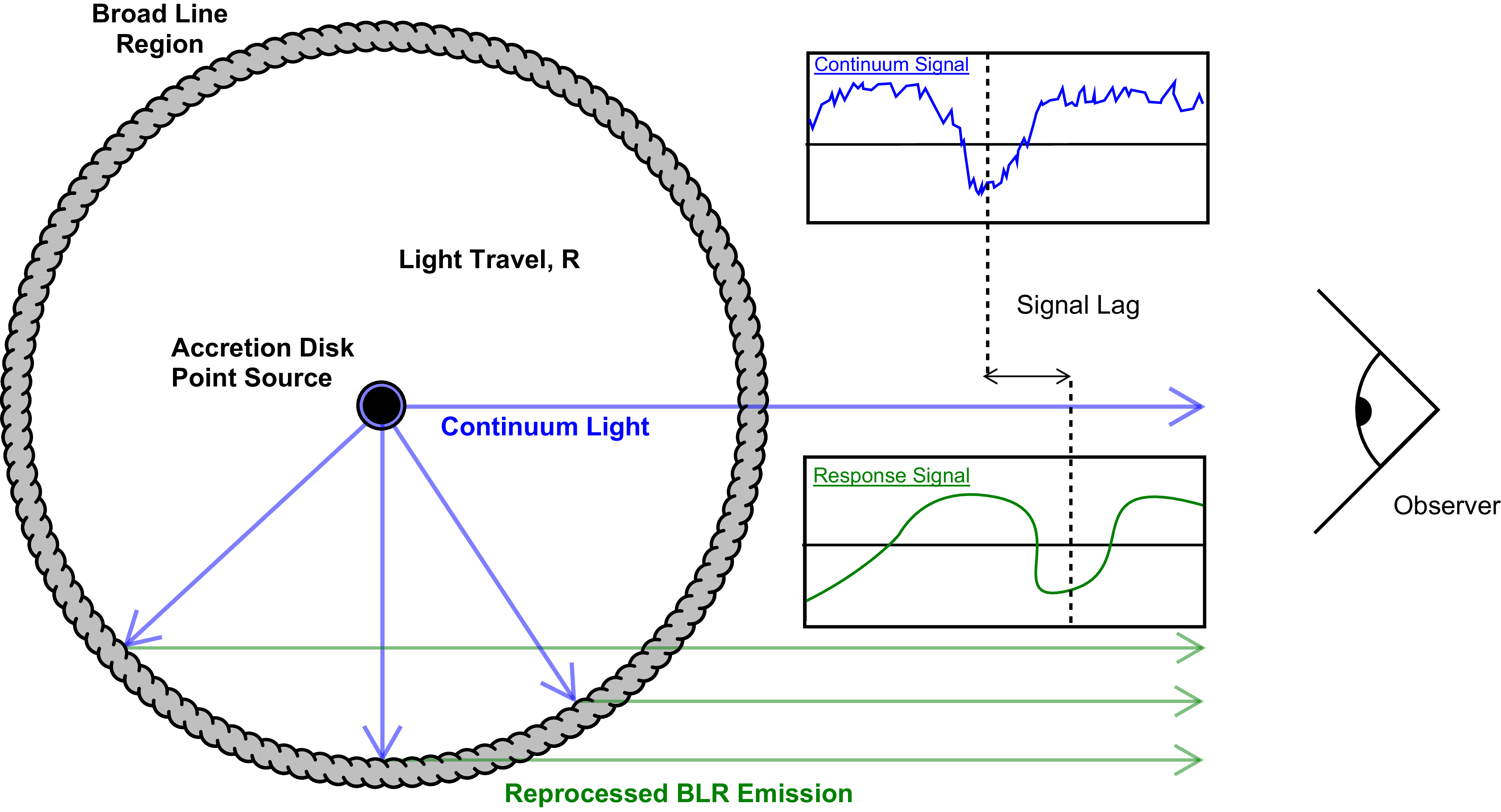
 ⟨f⟩
⟨f⟩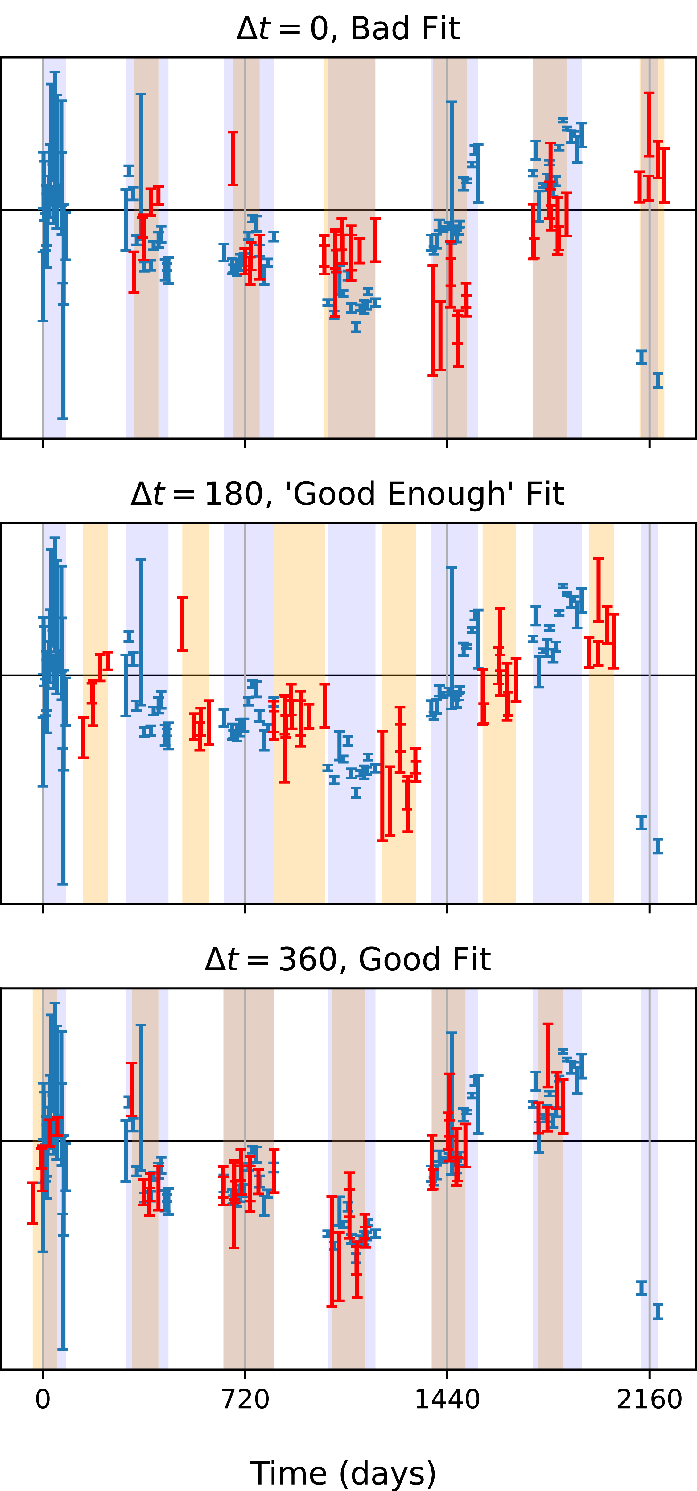
 360d
360d ≈180d
≈180d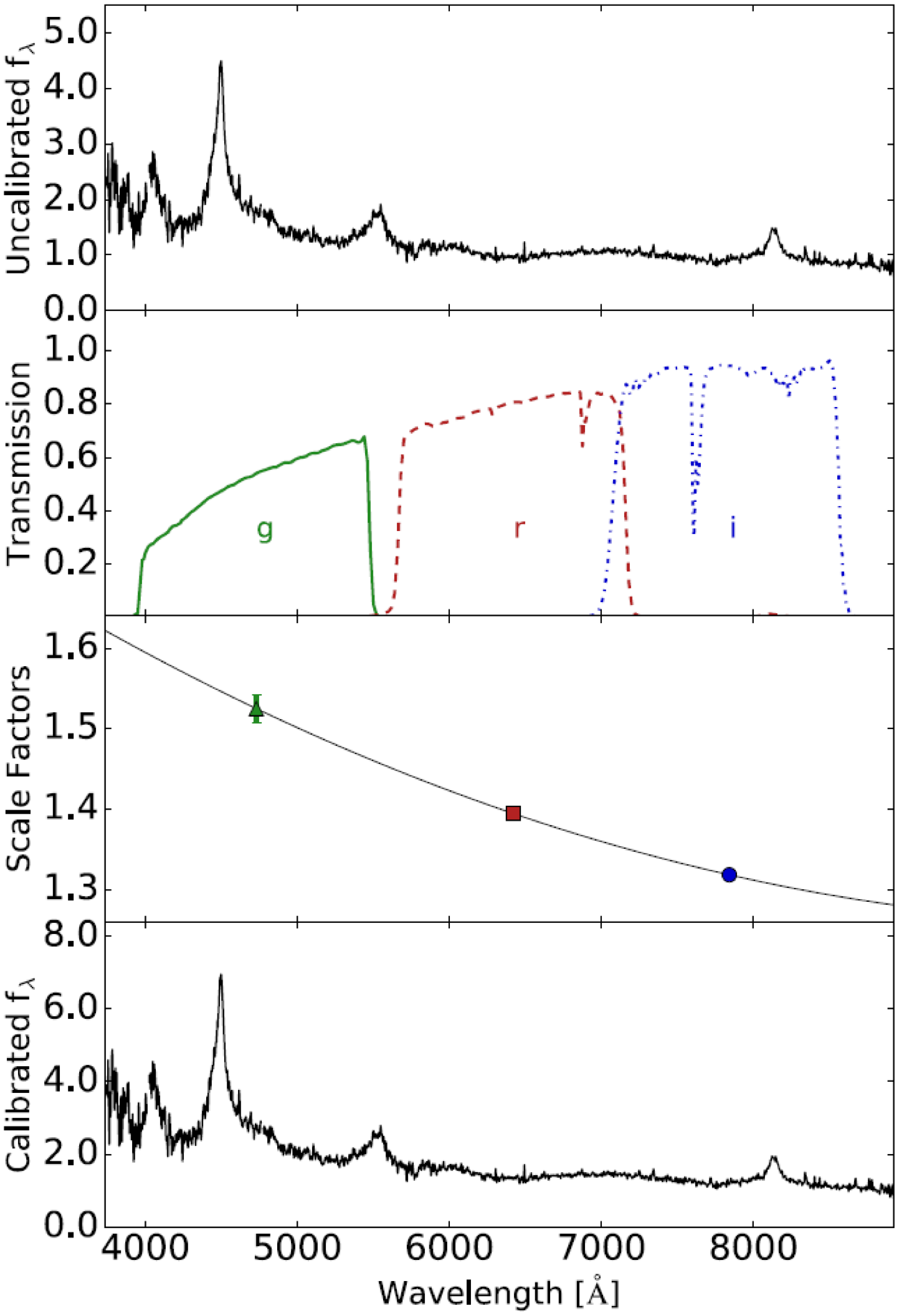
 10−16ergs−1cm−2Å−1counts−1
 10−16ergs−1cm−2Å−1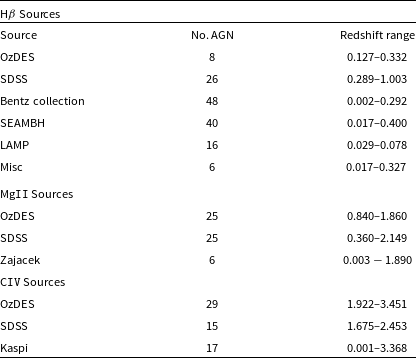
 R−L
R−L
 R−L
R−L β
β log10
log10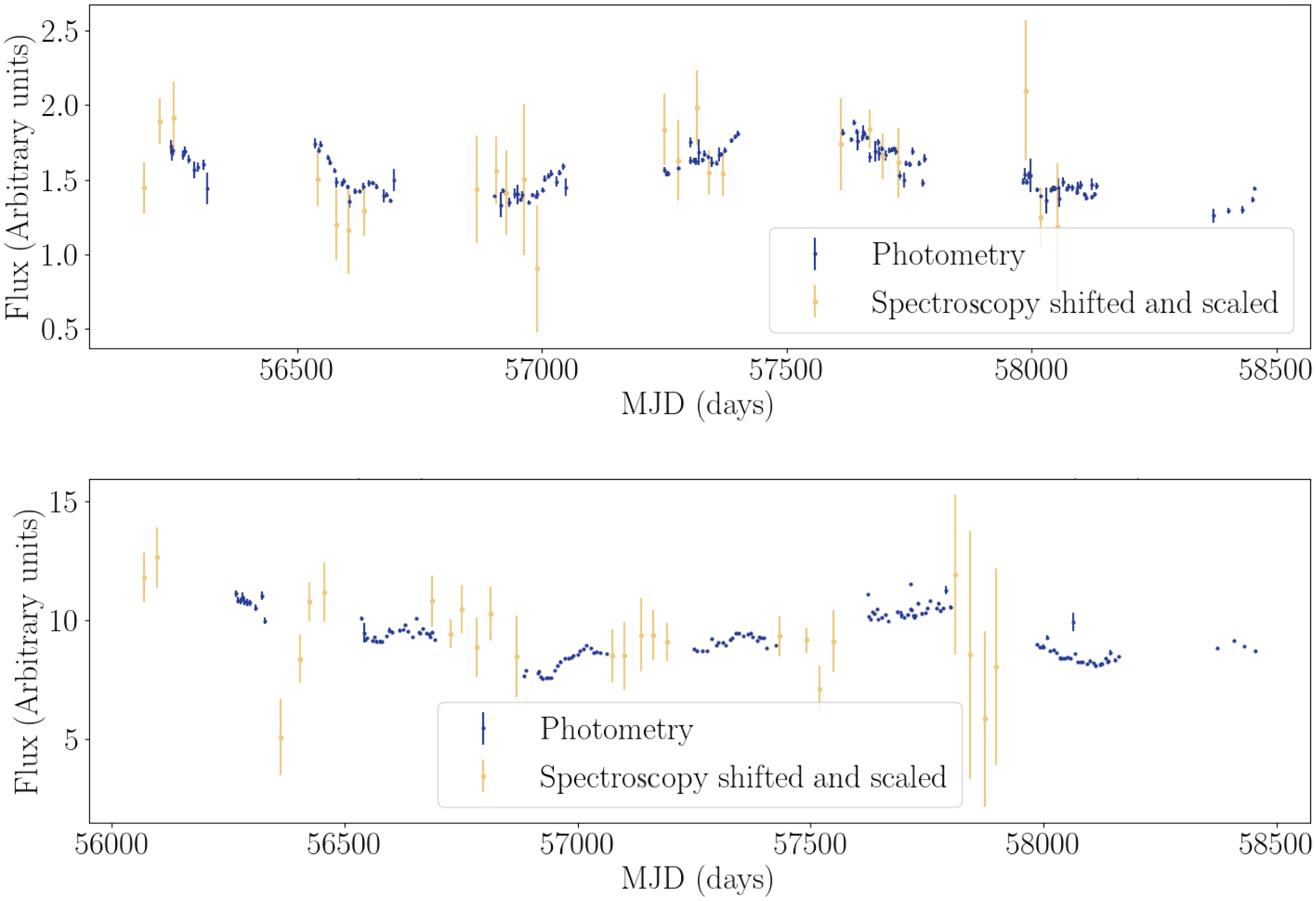
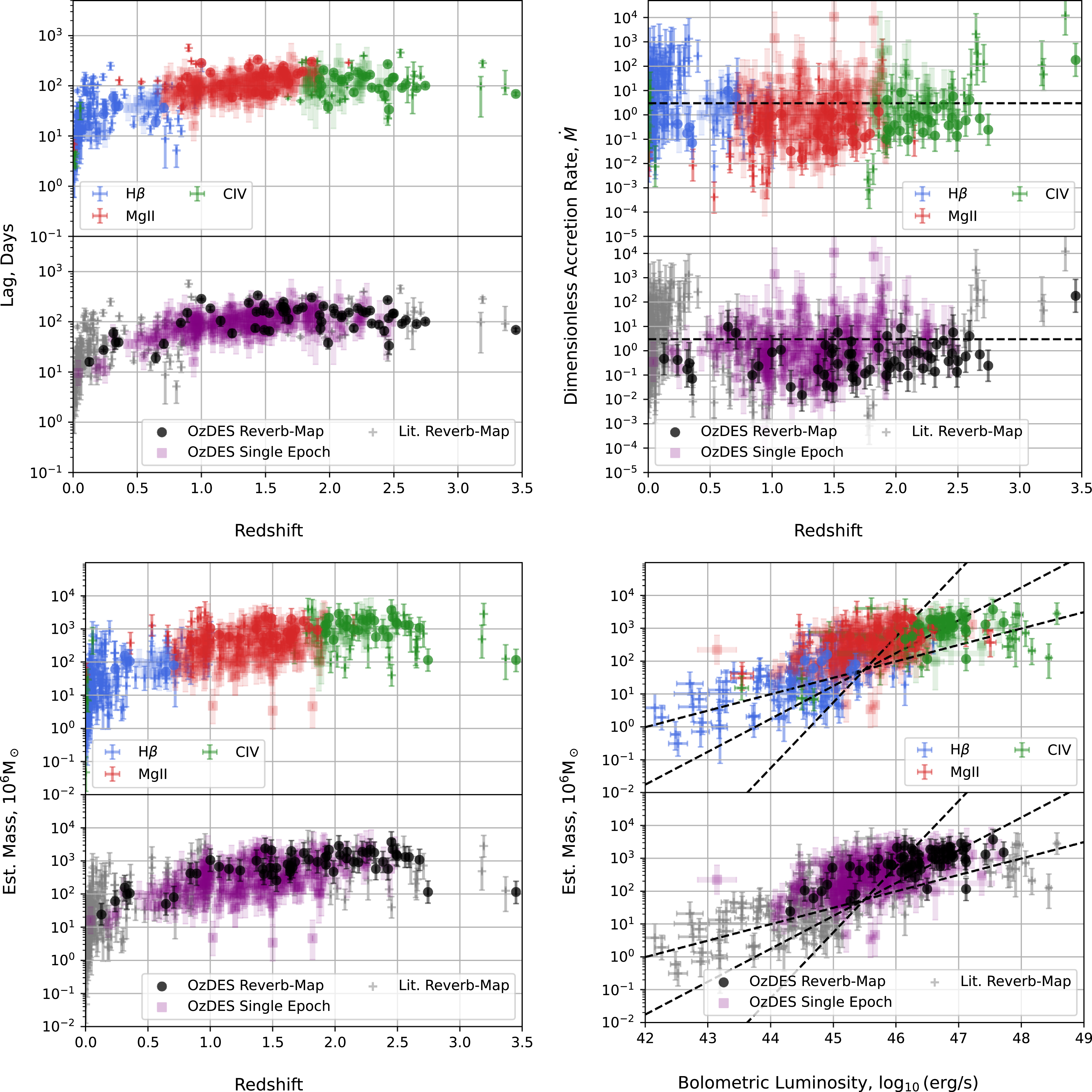
 0.5,1.0
 2.0
2.0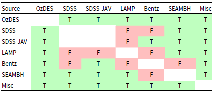
 β
β R−L
R−L 2σ
2σ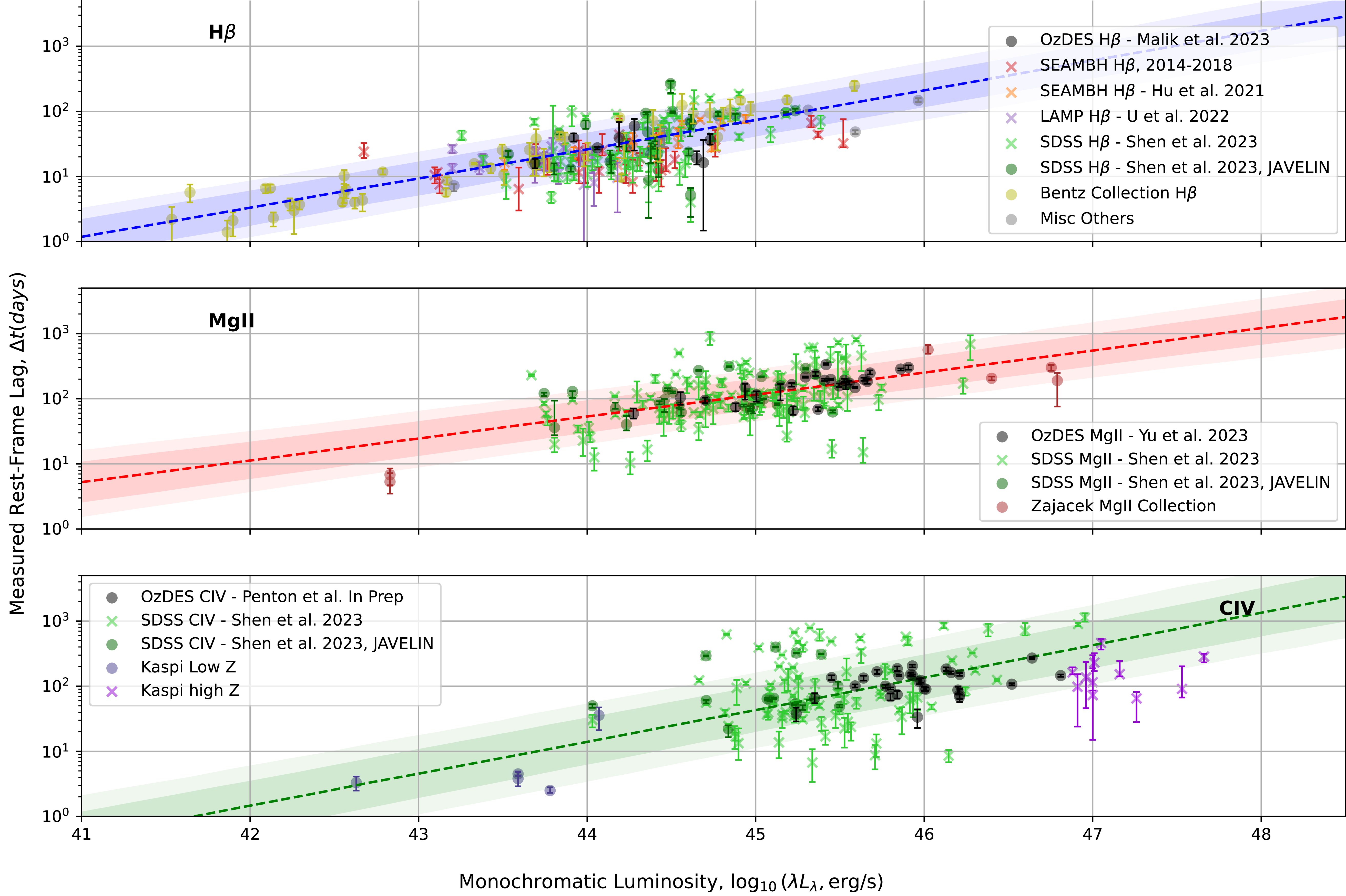
 R−L
R−L R−L
R−L β
β R−L
R−L 5100Å
5100Å 3000Å
3000Å 1350Å
1350Å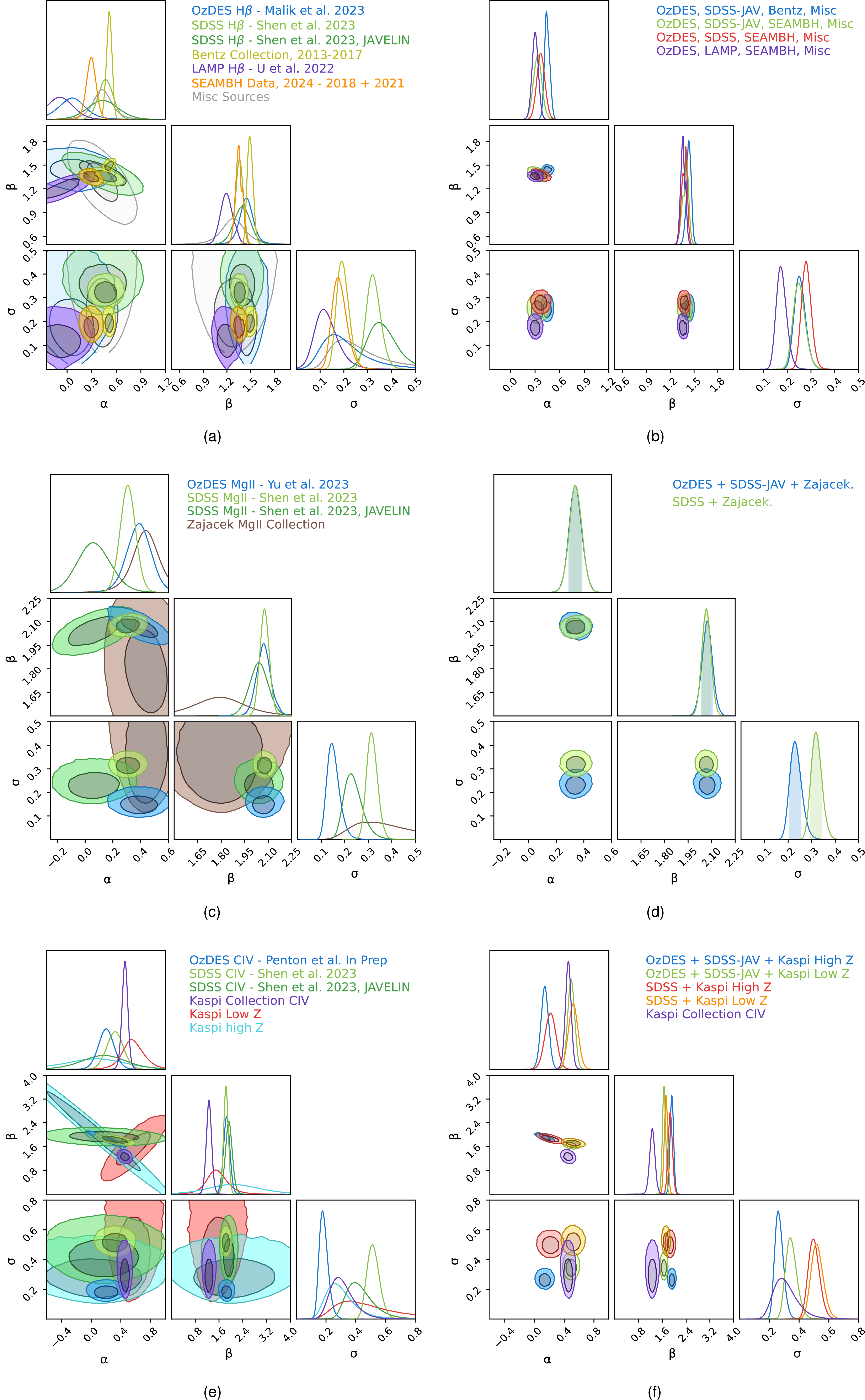
 R−L
R−L β
β α
α β
β 1044erg/s
 β
β 1045erg/s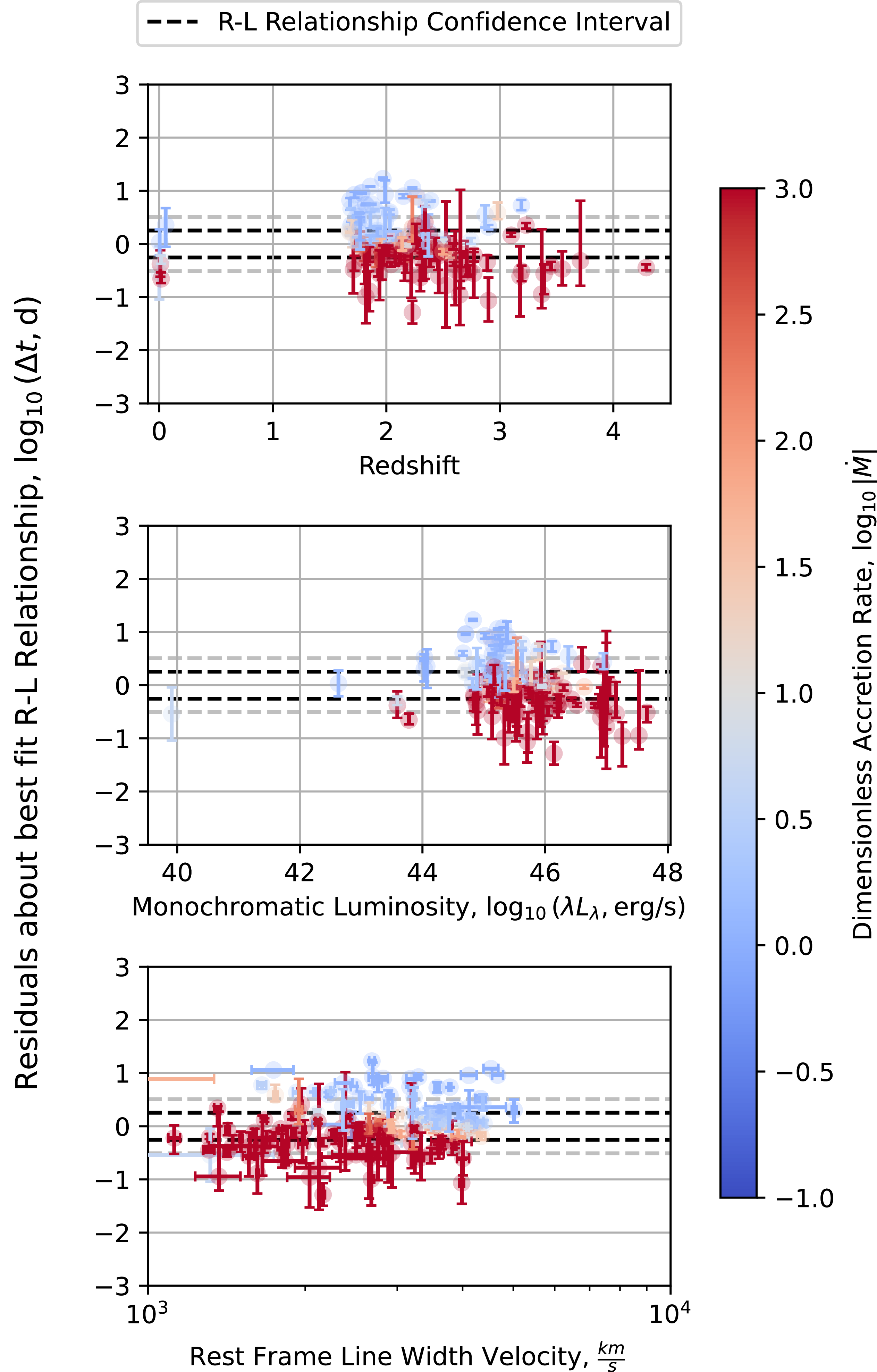
 R−L
R−L log10(M˙)
 R−L
R−L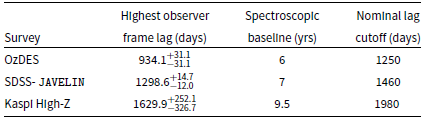
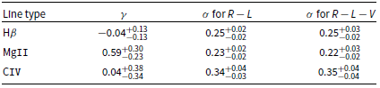
 R−L
R−L γ=0
γ=0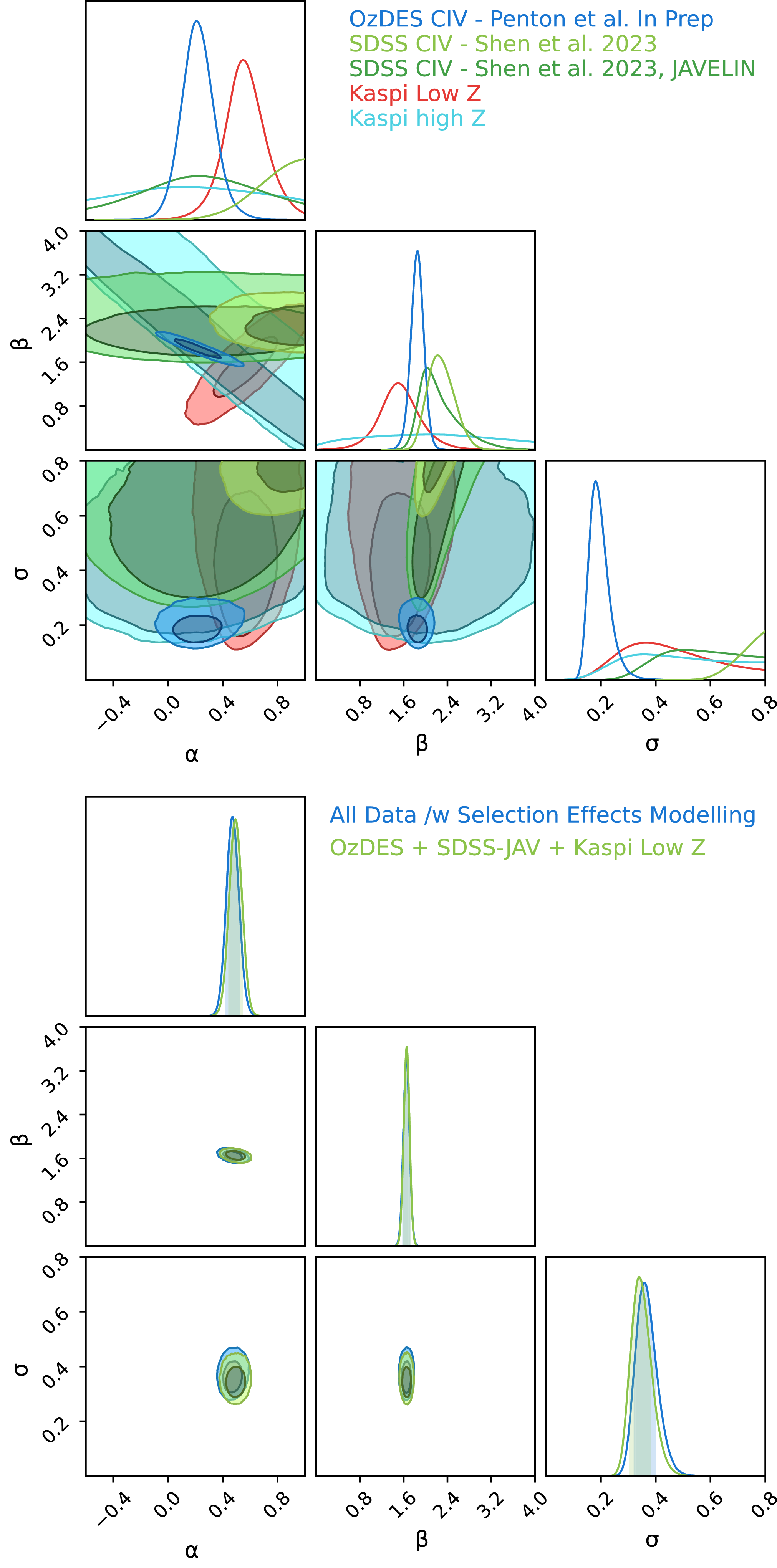
 R−L
R−L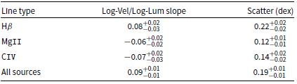
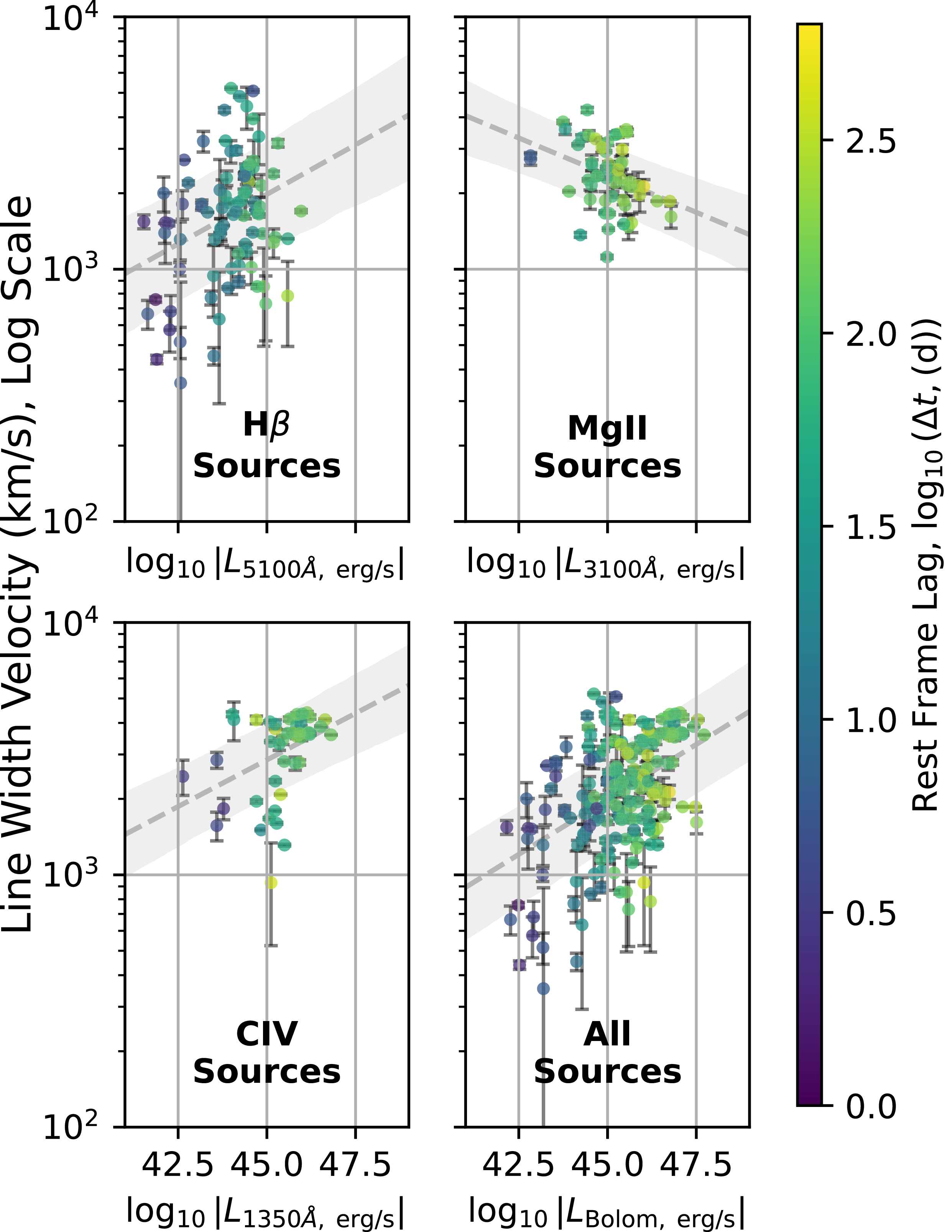
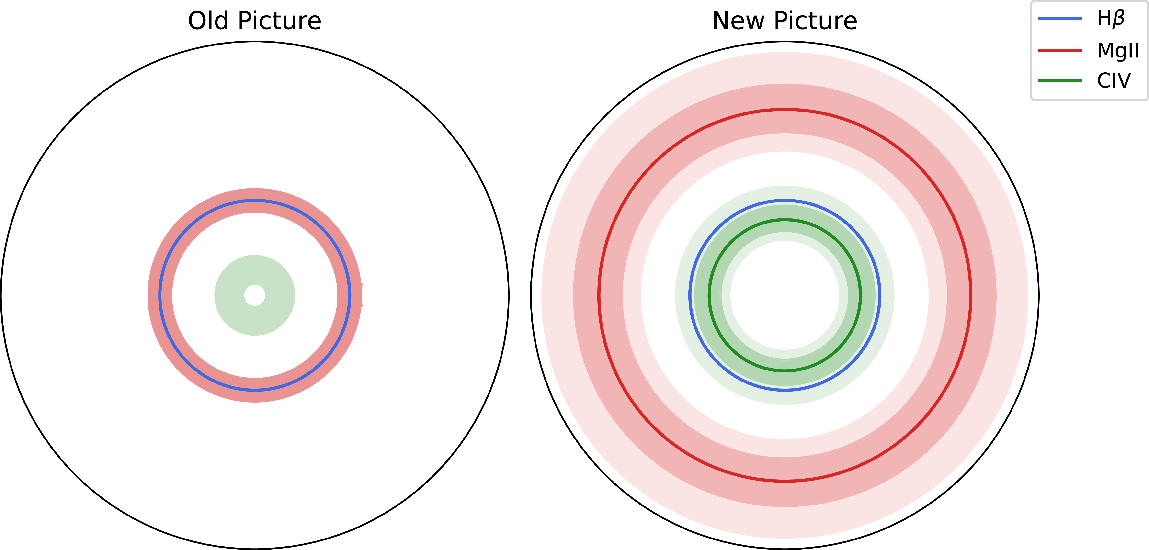
 β
β β
β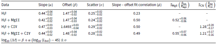
 R−L
R−L 1045erg/s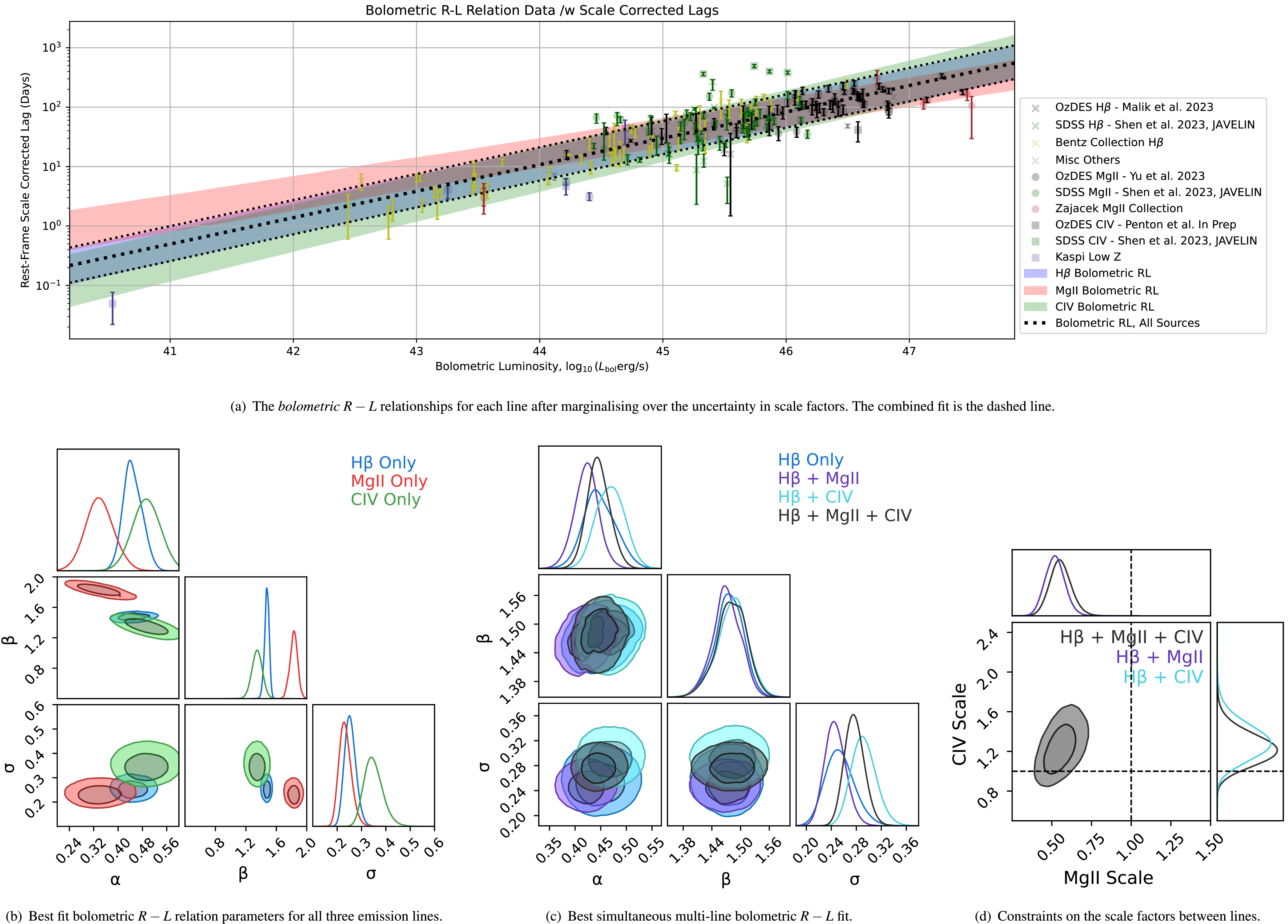
 R−L
R−L R−L
R−L R−L
R−L β
β R−L
R−L R−L
R−L β
β CMgII≈1
 CCIV≈1
 β
β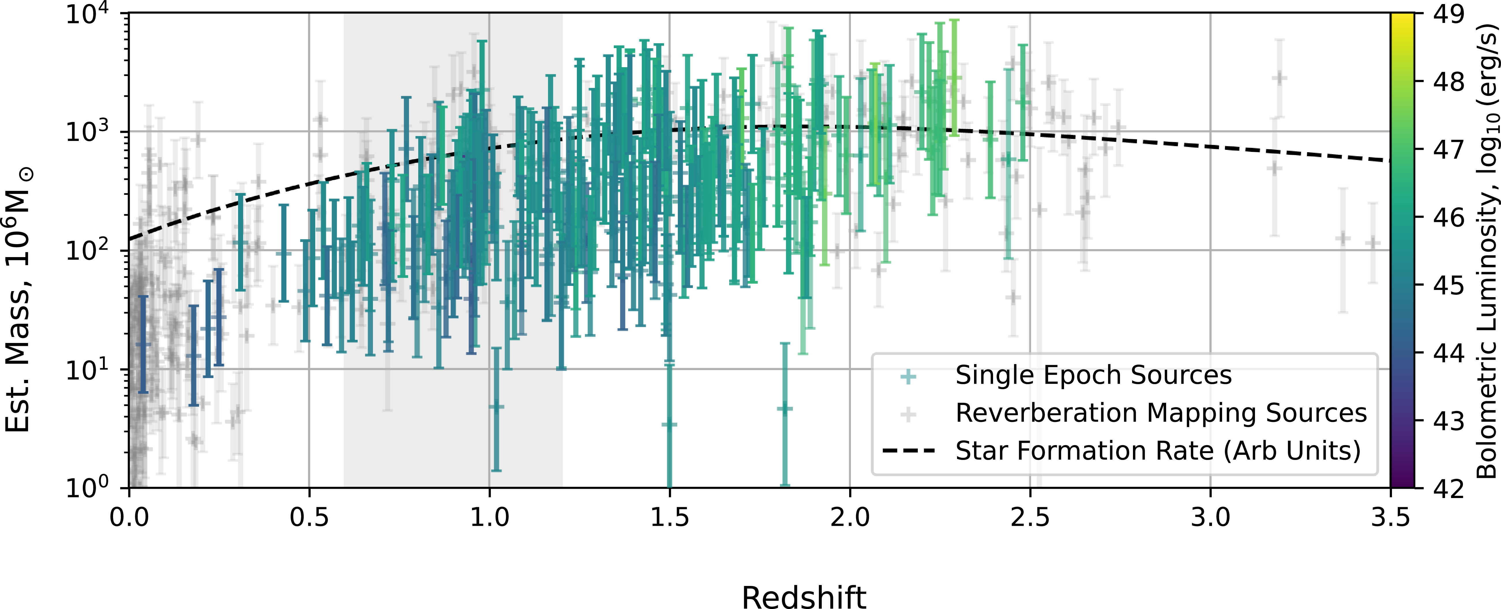
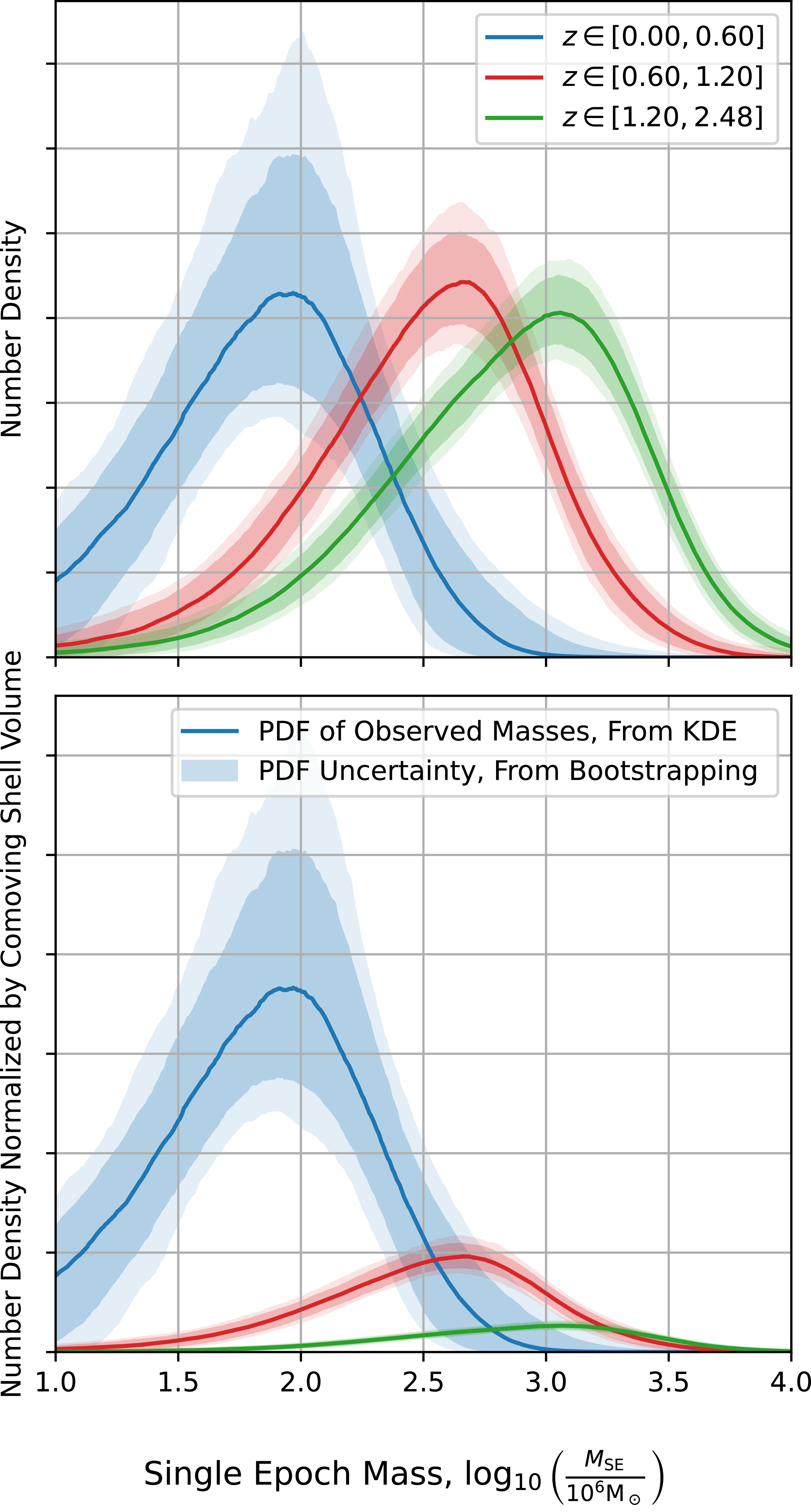
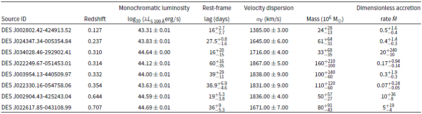
 β
β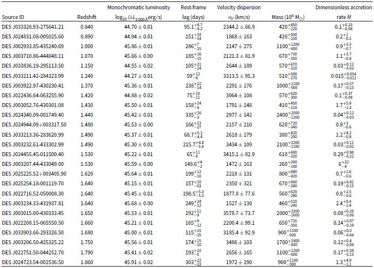
 λL3000Å
 λL5100Å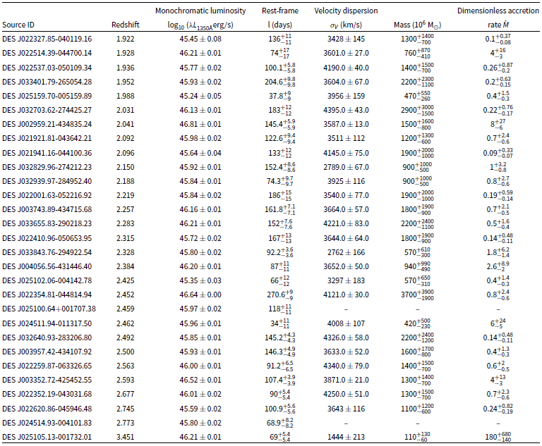
 λL1350Å
 λL5100Å
 R−L
R−L β
β 5100Å
5100Å 3000Å
3000Å 1350Å
1350Å β
β 5100Å
5100Å
 Open access

