





Introduction
Third sector associations (TSAs), also referred to as the voluntary or non-profit sector or civil society, can be defined to operate in a distinct “sector of organised human action composed of collective actors beyond the family and distinct from the state and the market” (Viterna et al., Reference Viterna, Clough and Clarke2015, p. 175). As such, while the public sector naturally sets the laws and regulations under which TSAs operate, in democratic countries, the government does not directly control the sector. Further, the clearest distinction between the private and the third sector can be drawn based on the non-profit and for the public good nature of TSAs compared to the often profit-seeking nature of the private sector (Bryson et al., Reference Bryson, McGuiness and Ford2002). The third sector is highly heterogeneous and diverse (Salamon & Sokolowski, Reference Salamon and Sokolowski2016), ranging from very small local associations to large international organizations active in a variety of different sectors of society. This wide-ranging nature of the third sector thus cautions against attempts to measure the sector (Bryson et al., Reference Bryson, McGuiness and Ford2002), which Kendall and Knapp (Reference Kendall, Knapp, Smith, Rochester and Hedley1995) described as a “loose and baggy monster.”
Notwithstanding the critical voices against mapping it, the question of the size of the third sector is alluring. According to Salamon et al. (Reference Salamon, Sokolowski and List2003), the sector is one of the most significant economic forces in contemporary society. Consequently, over the years, the third sector has received ample academic interest from the perspectives of its role in (co-)producing public services and its impacts on regional development, welfare, and social capital, etc. (e.g., Birch & Whittam, Reference Birch and Whittam2008; Pestoff, Reference Pestoff2012; Terzo et al., Reference Terzo, Notarstefano and Di Maggio2023). Similarly, policymakers have laid increasing emphasis on incorporating third-sector actors into regional development work due to their role in maintaining and enhancing regional vitality, including economic but also wider aspects of the well-being and communal participation of local populations (Makkonen & Kahila, Reference Makkonen and Kahila2021). This trend has occurred in tandem with the austerity-induced withdrawal of the public sector from many spheres of society, particularly in rural regions (Bock, Reference Bock, Scott, Gallent and Gkartzios2019; Lehtonen et al., Reference Lehtonen, Makkonen, Vihinen, Hirvonen, Rautiainen and Voutilainen2025; Makkonen et al., Reference Makkonen, Lehtonen, Inkinen, Vihinen and Voutilainen2025). Indeed, as presented by Matthies (Reference Matthies2007), the third sector is emphasized as being a part of the solution to several local societal challenges relating to access to services, local democracy, community culture vitality, and the adequacy of public funds. Thus, the importance of the role the third sector plays in society has been recognized by both academia and policymakers.
While the recognition of the rising importance of the third sector can be generally considered as a positive development, the reasons behind this change can be traced to fiscal austerity. The increasing role that the third sector is expected to play in regional development has also been criticized from the perspective of offloading responsibilities from the shoulders of the public to the third sector without proper compensation. Indeed, influenced by neoliberal voices calling to reduce the role of the state in the economy and amplified by the financial burden of keeping up the welfare state in times of economic crisis, we have witnessed a withdrawal of the public sector, particularly from depopulating rural and peripheral regions (Lehtonen et al., Reference Lehtonen, Makkonen, Vihinen, Hirvonen, Rautiainen and Voutilainen2025; Milligan, Reference Milligan2007).
In tandem with the diminishing role of the public sector in providing services to citizens, the third sector is increasingly expected to take a role in welfare and cultural and recreational service provision (Fyfe & Milligan, Reference Fyfe and Milligan2003)—a change that has been referred to as the “associational revolution” (Salamon, Reference Salamon1999)—which would imply that rural regions have a greater need for TSAs to compensate for the loss of the withdrawal of the public sector. This, however, raises concerns: if the vitality of regions is increasingly dependent on TSAs it would be undermined if the potentially localized and uneven geography of the third sector favor urban locations (Bryson et al., Reference Bryson, McGuiness and Ford2002). Uneven geography refers to commonly observed subnational regional differences in the development of the economy and its different sectors (Christophers, Reference Christophers, Kitchin and Thrift2009); an issue explored here with regard to TSAs. The above discussion acts as an important motivation behind the approach of this study to compare the third sector in urban versus rural locations.
The literature on the third sector, focusing on charity, philanthropy, community organizations, and voluntarism (e.g., Evers & Laville, Reference Evers and Laville2004; Halford et al., Reference Halford, Leonard and Bruce2015; Mohan & Bennett, Reference Mohan and Bennett2019) has given salience to the research field. Nonetheless, and despite the evident importance of such research, the geography of the third sector has been rarely studied (see MacIndoe & Oakley, Reference MacIndoe and Oakley2023, for a recent literature review) from the perspective of urban–rural differences. Consequently, relatively little is known about the potential distributional differences of TSAs between urban and rural locations. As stated by Fyfe and Milligan (Reference Fyfe and Milligan2003), there is a continuing scarcity of empirical data on the third sector and, thus, an ongoing need for mapping the sector, as contributed by this paper. As such, this paper answers a recent call by MacIndoe and Oakley (Reference MacIndoe and Oakley2023) for further studies on the third sector from a spatial perspective. In doing so, the paper seeks to answer the following research questions that, given the importance of the third sector in promoting regional vitality, also have clear policy relevance for regional development work:
-
• Are there differences between urban and rural regions in the distribution of TSAs?
-
• What factors are associated with the potentially uneven geographical distribution of the third sector between urban and rural regions?
The paper seeks to answer the above questions with data from Finnish municipalities representing the local level of administration in Finland. As a Nordic welfare state (Salamon & Anheier, Reference Salamon and Anheier1998) undergoing changes in the role of the third sector (Ruuskanen et al., Reference Ruuskanen, Jousilahti, Faehnle, Kuusikko, Kuittinen, Virtanen and Strömberg2020), Finland offers an interesting location for analyzing the geography of the third sector. According to Saukkonen (Reference Saukkonen2013), TSAs have been among the key sources for both national and regional identity building in Finland, thus explaining their popularity. Membership of TSAs is common among Finns. Indeed, as outlined by Harju (Reference Harju2020), the roots of the Finnish third sector can be traced back to the late 19th century and to the idea of nationhood, where civic activity created a sense of national identity, leading to Finns declaring the nation an independent state in 1917. TSAs remained common even though the modernization of Finland from the late 1950s decreased the population’s willingness to partake in third sector activities. Therefore, while many traditional TSAs experienced a downturn, overall, there was no real decline in civic activity. The 1970s were a time of strong social organization in Finland as political competition led to the establishment of hundreds of new TSAs.
More recently, the position of professional and political associations has weakened as people’s interests have turned more towards pastime, sports, and cultural and environmental issues. This has been reflected in the rapid growth in the number of leisure and lifestyle associations. This has placed service provision in a secondary role (Matthies, Reference Matthies2007) to other functions of the third sector (e.g., leisure activities, representing and advocating for specific groups). However, not much is known about the geography of the third sector in Finland beyond qualitative and rather anecdotal evidence of higher “community spirit” ( talkoohenki ) in the rural regions of Finland (Alanko et al., Reference Alanko, Kilpi, Ahola, Mäenpää and Faehnle2024).
Due to these historical ties, the relationship between the public and the third sector in Finland is described as close and symbiotic (Ruuskanen et al., Reference Ruuskanen, Jousilahti, Faehnle, Kuusikko, Kuittinen, Virtanen and Strömberg2020). TSAs are still thriving in Finland in the early 21st century. However, the depopulation and aging of the remaining population of large parts of Finland nowadays challenge the continuation of TSAs. At the same time, the Finnish local government landscape has been in a state of flux in the 21st century. Finnish municipalities have traditionally had a strong role in providing welfare, cultural, educational, and social services mandated by law and financed by the state and taxes paid to the municipality by its residents and local businesses.
Recently, the responsibility for organizing health, social, and emergency services in Finland was transferred to newly established regional wellbeing service counties, mainly justified by the expected cost-effectiveness of the new system. However, due to the shrinkage of the local population and economy and subsequent financial austerity faced by many Finnish regions, the government is keen to see TSAs take an even greater role in providing welfare services and revitalizing community participation and culture. Yet, at the same time, the Finnish government has been cutting its financial aid to many TSAs, which has had a substantial impact on the third sector and its operating conditions. Local authorities have, however, been generally willing to financially support TSAs, since such funding is seen as a cost-effective way to improve regional vitality (Makkonen & Kahila, Reference Makkonen and Kahila2021).
The remainder of this paper is organized as follows. First, a review of previous literature is presented to elaborate on the relevance of the study and the chosen empirical approach. Second, the utilized indicator depicting TSAs and variables explaining the reasons behind their potentially varying prevalence in urban and rural settings are introduced, followed by a discussion on the methodological choices of this paper. Third, the most relevant results are laid out showing that socio-economically less advantageous rural regions host the most TSAs per capita. The concluding section summarizes the main findings, discusses the theoretical and practical implications of the results, and considers the limitations of the chosen approach.
Uneven geography of the third sector? Demand and supply side explanations and urban–rural differences
As reviewed by Salamon and Anheier (Reference Salamon and Anheier1998), several theories exist that help us hypothesize the reasons behind the potentially uneven geography of the third sector. The government failure theory indicates that people will turn to third sector organizations in situations where desired goods are not supplied by the public or private sector. By implication, the higher the demand, the larger the third sector. The theory aligns with the contemporary situation where the public sector has been withdrawing, particularly from rural regions, due to financial austerity (Bock, Reference Bock, Scott, Gallent and Gkartzios2019; Lehtonen et al., Reference Lehtonen, Makkonen, Vihinen, Hirvonen, Rautiainen and Voutilainen2025; Makkonen et al., Reference Makkonen, Lehtonen, Inkinen, Vihinen and Voutilainen2025). According to the welfare state theory, extensive state provision of services should result in a small third sector. According to the interdependence theory, close cooperative relationships can be forged between the public and the third sector, and, thus, there should be a positive relationship between them, implying that TSAs benefit from external financial resources. Finally, the social origins theory treats the third sector as a complex social system forged by historical forces and dependent on different political regimes (Salamon & Anheier, Reference Salamon and Anheier1998).
The above theories stem mainly from the US-centric research tradition and do not entirely fit the case of Finland. For example, contrary to the welfare state theory, Finland has both a large public and a large third sector (Matthies, Reference Matthies2007). Nonetheless, particularly the government failure and interdependence theories offer a theoretical motivation for focusing on the supply of and demand for the third sector, i.e., whether the presence of TSAs is at least partly explained by socio-economic conditions. It is fully acknowledged that the empirical approach applied here cannot measure the whole spectrum of reasons behind the home location of registered TSAs. Indeed, there are a variety of factors that have been stated to lie behind the potential uneven geography of the third sector. Previous studies have underlined: 1) the importance of local histories, 2) the role of temporal changes in national welfare policies and their local consequences, and 3) the role of individuals and their place attachment, behind the founding of TSAs in specific locations (Milligan, Reference Milligan2007).
While there are no comparative regional statistical data that would cover all municipalities, at least in Finland, on, e.g., place attachment or TSAs’ location history, there are a range of measurable socio-economic factors potentially affecting the regional spread of the third sector, including: 1) variation in social needs (demand side argumentation) and 2) economic health (supply side argumentation). First, as summarized by Fyfe and Milligan (Reference Fyfe and Milligan2003) and in line with the government failure theory, a heightened regional need for social services and assistance has been noted to create pressures and demand for the voluntary sector. According to the demand side explanation, this higher need is expected to lead to a higher concentration of TSAs in socially deprived regions rather than well-off regions. Second, in line with the interdependence theory, there are evident variations between local government support for third sector activity (Clifford et al., Reference Clifford, Geyne-Rahme and Mohan2013). Further, the private sector (including households) can also provide helpful financial resources to the third sector. Indeed, the economic development level of regions has been discussed to affect the donative resources available from local workers and corporations, which in turn affects the “operational environment” of TSAs (Fyfe & Milligan, Reference Fyfe and Milligan2003). As such, in some regions the third sector might be relatively better financed than in others. Thus, in the supply side explanation, it is expected that the presence of TSAs is higher in economically more developed regions than in less developed ones.
While reviewing the entirety of empirical papers on the topic is beyond the scope of this paper, one can find results from the extant literature supporting both explanations—but not unanimously. For example, Yan et al. (Reference Yan, Guo and Paarlberg2014) have shown that indicators proxying higher demand have a significant positive effect on the average number of TSAs in regions. Similarly, Peck (Reference Peck2008) has provided empirical evidence supporting the demand side explanation: i.e., that TSAs locate in regions of greater need. In line, for example, Joassart-Marcelli and Wolch (Reference Joassart-Marcelli and Wolch2003) as well as Bielefeld (Reference Bielefeld2000) have shown results pointing to regional differences in the presence of the third sector caused by variations in metropolitan wealth. Their results indicated that wealthier sites with higher socio-economic status had a larger third sector in terms of the number of TSAs they host. Moreover, local government expenditure was associated with higher third sector activity (Joassart-Marcelli & Wolch, Reference Joassart-Marcelli and Wolch2003).
Another potential explanation for the potentially uneven geography of the third sector stems from the inherent differences between urban and rural regions. Notably, urban regions are often characterized to have lower levels of community engagement than rural regions (Hooghe & Botterman, Reference Hooghe and Botterman2012). This would indicate that, in relative terms, rural regions are the more likely home regions for TSAs compared to urban regions. Further, while traditionally there has been very little non-institutional, non-association-based civic activity in Finland (Harju, Reference Harju2020), according to Mäenpää and Faehnle (Reference Mäenpää and Faehnle2017: 78) in urban settings, engagement increasingly occurs through less formal civic activism (labeled as the fourth sector) that they define as “the area of civil society that, with its quick, lightly organised, proactive and activity-centered nature, is structured outside of the third sector.”
The evidence is, however, mixed. While Hooghe and Botterman (Reference Hooghe and Botterman2012) did not find evidence to support the existence of an urban–rural divide vis-á-vis participation in TSAs, Paarlberg et al. (Reference Paarlberg, Nesbit, Choi and Moss2022) found that rural respondents are more likely to report volunteering compared to urban respondents. Again, while Yan et al. (Reference Yan, Guo and Paarlberg2014) have evidenced that TSAs are more likely to locate in urban regions, Marchesini da Costa (Reference Marchesini da Costa2016) presents results that support an opposite interpretation, i.e., high numbers of TSAs in regions with a high proportion of rural population. In addition to the “density” of the third sector, another interesting issue concerns the driving forces behind their location in urban vs rural regions. As stated by Lecy and Van Slyke (Reference Lecy and Van Slyke2013), the processes that drive third sector formation in rural regions may be distinct from processes driving third sector density in urban regions.
The above discussion, controversy, and lack of consensus underline the importance of bringing the regional (subnational) scale into the analysis of the third sector to create a framework for the study and understanding of its spatial spread by taking into account urban–rural differences. Specifically, based on the above theories and empirical evidence, the paper sets out to test whether urban or rural regions are more prone or averse to host TSAs and whether socio-economic factors related to the demand and supply side arguments differently affect the geography of the third sector in these regions.
Data and methods
Indicator selection
Finnish third sector associations
In Finland, a TSAs can be founded for the common realization of a non-profit purpose (Finnish Patent and Registration Office, 2023). They can register themselves in the Finnish Register of Associations to become legal entities and, as a result, enter into contracts in the name of the association, own property, and act as entities for legal purposes. These registered associations are governed by the Finnish Associations Act (1989/503). There are also less formal TSAs (networks or movements) that have not registered themselves. These unregistered associations are not legal entities and have no legal capacity. They can, however, e.g., carry out limited fundraising (Järjestöhautomo, 2023). It has been estimated that the number of unregistered associations in Finland likely ranges in the thousands—one commonly cited figure being 30,000 (Harju, Reference Harju2010). However, there are no exact statistics on unregistered associations. Therefore, the data utilized here pertains to registered associations.
The Finnish Patent and Registration Office (PRH) was approached and specifically requested to provide data on TSAs per their home municipalities. In total, the data provided by the PRH included location data on 79,461 currently active (in 2022) TSAs in Finland. The TSAs were allocated to specific municipalities according to their home locations and normalized per municipal population (Table 1) including party-political, professional, social, health, culture, leisure, sports, religious, national defence, and international relationship associations. The number of TSAs in these specific sub-categories is, however, very small or in many cases zero for the smaller Finnish municipalities (in terms of population). As discussed by Putnam (Reference Putnam1993), the density of TSAs can be regarded as positive and as a proxy for the activity level of local civil society. Therefore, a decision to use the aggregate number of TSAs per capita was made, influenced by key methodological considerations: the quantitative methods discussed below do not work well with datasets that include several missing (zero) observations.
Indicator selection, definitions, and data sources

Table 1. Long description
The table is organized into three main sections.
1. Supply Indicators:
- Education: Highly educated persons as a percentage of the adult population (2018–2022), including tertiary education levels. Source: StatFin.
- Turnover: Firm turnover in thousand Euros per firm (2018–2022), representing sales profits after deductions. Source: StatFin.
- Municipal allowances: Financial support in Euros per population (2020–2022), including grants and subsidies. Source: Tutkihallintoa.
2. Demand Indicators:
- Unemployment: Unemployed people as a percentage of the labor force (2018–2022), covering ages 16–64. Source: StatFin.
- Health (morbidity): Morbidity index (2019–2022) indicating prevalence of illnesses compared to a national average of 100. Source: Sotkanet.
- Income (poverty): Risk of poverty rate as a percentage of the population (2018–2022), based on 60 percent of median disposable income. Source: StatFin.
3. Other variables:
- Urban–rural status: A dummy variable based on 2022 classification into four types: sparsely populated rural areas, rural heartland areas, rural areas close to urban areas, and urban areas. Source: Y K R.
- Associations: Third sector non-profit associations per thousand inhabitants (2022). Source: P R H.
Notes: Sotkanet is a statistical database maintained by the Finnish Institute for Health and Welfare; StatFin is a statistical database maintained by Statistics Finland; Tutkihallintoa is a data interface maintained by the State Treasury of Finland; YKR is a geoinformation database maintained by the Finnish Environment Institute; Data on associations were obtained from the Finnish Patent and Registration Office (PRH). The descriptions of the variables come from the above sources.
A further point of clarification is the trade-off inherent in normalizing the number of TSAs per municipal population. On the one hand, the normalization puts smaller municipalities in an advantaged position with regard to the number of TSAs as each municipality tends to have a certain “basic set” of TSAs. The Martha organization (https://www.martat.fi/in-english/), providing advice in home economics, provides an illustrative case of the problem. The Martha organization has hundreds of local registered TSAs all around Finland. They range in size from tens to hundreds of members. The largest ones are generally situated in and around the capital region of Helsinki and other large Finnish urban centers. Irrespective of their size, all Martta associations “count” equally in the municipal data. Thus, it is acknowledged that, on the one hand, normalizing the data has clear drawbacks. On the other hand, analyzing the absolute numbers of TSAs in Finnish municipalities, whose population sizes range from less than 1,000 to almost 700,000, has even more severe methodological shortcomings.
Socio-economic factors: Demand and supply side variables and urban–rural classification
As discussed above, from the supply side, the availability of economic resources in a region is expected to affect the third sector positively. Thus, the supply side argument was operationalized via different sectors: households as well as private sector (firms) and local (municipal) government variables as the main sources for donative resources. The share of highly educated population was utilized to measure the economic resources of households due to the well-documented link between education and income (Tokila & Tervo, Reference Tokila and Tervo2011). Firm turnover (per company) was used to proxy private sector resources and municipal spending on grants and allowances (per population) for public sector resources (Table 1). Naturally, the focus on financial/economic resources as proxies for supply leaves out other relevant aspects, such as volunteering. Analyzing this human resource component of supply would, however, necessitate the use of data on TSAs membership and activity, which, unfortunately, is unavailable at the level investigated here.
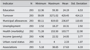
In terms of variables describing demand, social needs are often tied to economic conditions. Therefore, the concept of “deprivation” was used for operationalizing the regional variation in these dimensions (Clifford et al., Reference Clifford, Geyne-Rahme and Mohan2013). That is, the indicator selection was based on finding similar underlying indicators of deprivation for the Finnish context that are in use in other countries (Ministry of Housing, Communities, & Local Government, 2019). These indicators include unemployment figures as well as health (morbidity) and income (poverty) related deprivation (Table 1). Descriptive statistics are presented in Appendix Table A1. Naturally, the chosen indicators mainly focus on the service provision function of TSAs, disregarding their role, for example, in community culture. However, while there are scattered data on attendance in various cultural and sports events, such quantitative data as the demand for cultural services, recreational activities, and so forth does not exist at the municipal level in the Finnish context.
To avoid sporadic year-to-year variation, all the supply and demand variables were calculated as averages for five-year periods. However, due to missing data, the time period is three or four years for certain variables. Principal Component Analysis (PCA) was used to construct two indices: 1) supply index and 2) demand index. PCA is a very commonly utilized tool for managing information in large, correlated datasets (Makkonen & Inkinen, Reference Makkonen and Inkinen2015). It compresses the information contained by several variables into a single or a small number of principal component(s) but retains as much of the original information as possible. PCA produces weights that measure the “importance” of the included variables for the measured phenomenon. These weights are used for calculating, by following a regression logic, principal component scores (PCSs). Here, the PCSs measure the performance of Finnish municipalities in terms of the supply and demand side factors of third sector activity. For the PCA, municipal allowances and turnover variables were log (
$ {\mathit{\log}}_e $
 ) transformed. The PCA solutions passed the standard Kaiser-Meyer-Olkin (KMO) (> 0.6) and Bartlett’s tests for suitability (p < 0.001). Similarly, communalities (>0.3), eigenvalues (>1.0), and loadings (> 0.6) are above the standard thresholds for a suitable PCA solution (Jolliffe, Reference Jolliffe2002).
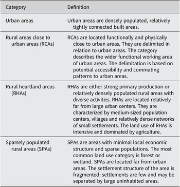
Finally, for distinguishing between urban and rural regions (Table 1) a decision was made to use the typology of the Finnish Environment Institute. The typology, which is utilized in Finland both for policy and academic purposes, is based on a detailed grid-level analysis (Helminen et al., Reference Helminen, Nurmio and Vesanen2020) and several demographic and socio-economic variables, including population, workforce and workplaces, buildings and dwellings, road network and commuting, as well as land use and coverage. At the municipal level, the categorization is aggregated to include four distinct groups of municipalities (see Table A2 for a detailed description): 1) sparsely populated rural areas (SPAs), 2) rural heartland areas (RHAs), 3) rural areas close to urban areas (RCAs), and 4) urban areas. While ca. 95% of the land area of Finland can be categorized as rural, roughly three out of four Finns live in urban areas, while almost four out of five workplaces are located in urban areas.
Mapping, comparisons and regression analysis
The mapping of TSAs per their home municipalities covering mainland Finland was conducted using ArcGIS software. Potential statistically significant differences in the number of TSAs were analyzed with non-parametric Spearman correlation and non-parametric Kruskal–Wallis tests—the latter is an extension to the Mann–Whitney U test for comparing more than two groups—to indicate differences in the distribution of TSAs between the supply and demand indices as well as between varying groups of municipalities.
To formally test the links between municipality categories (urban–rural), supply and demand indices, and the number of TSAs, a linear regression model was applied to the observed data (Schneider et al., Reference Schneider, Hommel and Blettner2010). Akaike Information Criterion (AIC) (Akaike, Reference Akaike, Petrov and Caski1973) and Bayesian Information Criterion (BIC) (Schwarz, Reference Schwarz1978)—both standard measures indicating the relative quality of statistical models (Cavanaugh & Neath, Reference Cavanaugh and Neath2019; Neath & Cavanaugh, Reference Neath and Cavanaugh2012)—were utilized in assessing the goodness of fit of the selected model.
Results
Mapping third sector associations in Finland
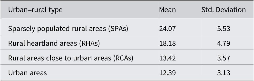
As seen from Figure 1, urban municipalities with large populations have high absolute numbers of TSAs, whereas proportionally the number of TSAs per capita is higher in rural municipalities with smaller populations (see also Appendix Table A3). Similarly, Figure 1 indicates a “divide” with generally higher per capita numbers of TSAs in the eastern and northern parts of the country, compared to coastal regions in southern and western Finland. However, there are also some individual municipalities with prominent third sector presence (in relation to population) that do not fit this general observation. Thus, while the maps in Figure 1 provide an interesting initial overview of the geography of the third sector in Finland, but they do not help us in formally determining what factors might be behind the uneven geographical distribution of TSAs. Therefore, the potential reasons behind the uneven geography of the third sector are discussed in greater detail below.
Regional characteristics (left) and absolute (middle) and relative size (right) of the third sector in Finnish municipalities.

Fig. 1. Long description
A three-panel map series of Finland.
Panel 1 (Left): Regional characteristics. The map is divided into four N U T S-2 regions: Northern and Eastern Finland, Western Finland, Southern Finland, and Helsinki-Uusimaa. Municipalities are categorized by size (Smallest to Largest using patterns) and urban-rural classification (Cities, R A C, R H A, and S P A using grayscale shading). Cities and R A C areas are concentrated in the South and West, while S P A and R H A areas dominate the North and East.
Panel 2 (Middle): Absolute size. Proportional circles represent the number of associations, ranging from 10 to 14,000. The largest circles are concentrated in the South, particularly around Helsinki-Uusimaa and major coastal cities in the West. The North has smaller, more dispersed circles.
Panel 3 (Right): Relative size. A choropleth map shows the number of associations per 1000 inhabitants across five tiers from 5.2 to 38.7. The highest densities (darkest shading) are found in the far North (Lapland) and specific clusters in Western and Southern Finland. The lowest densities (lightest shading) are primarily located in the rural heartland areas of the central and eastern regions.
Factors affecting the regional distribution of third sector associations
Descriptive approach
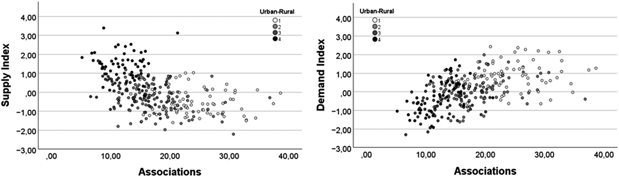
Concerning the potential link between supply and demand side variables and the uneven distribution of the third sector, measured as the number of TSAs per 1,000 inhabitants (Figure 2), in terms of supply, the higher the supply index score, the lower the number of TSAs in the region (Spearman’s correlation coefficient: −0.537; p-value <0.001). In terms of demand, the higher the demand index score, the higher the number of TSAs in the region (Spearman’s correlation coefficient: 0.522; p-value <0.001). In other words, whereas high supply is not connected with high third sector density, high demand is. Thus, it seems that regions with low scores in supply-side variables but high scores in demand-side variables host the most TSAs per population. The two indexes are only weakly correlated (Spearman’s correlation coefficient: −0.289; p-value <0.001). Thus, while they are connected, they are not direct substitutes for each other.
The relationship between supply and demand indices and the number of third sector associations (per 1,000 inhabitants). Urban–rural categories: 1 = sparsely populated rural areas (SPAs); 2 = rural heartland areas (RHAs); 3 = rural areas close to urban areas (RCAs); 4 = urban areas.

Fig. 2. Long description
A two-panel scatter plot. Both panels share a horizontal x-axis labeled Associations, ranging from ,00 to 40,00. The vertical y-axes range from -3,00 to 4,00. A legend in the top-right of each panel identifies four categories: 1 (white circle), 2 (light gray), 3 (dark gray), and 4 (black circle).
* Left Panel: The y-axis is labeled Supply Index. The data shows a negative correlation. Category 4 (urban) clusters in the top-left with high supply and low associations. Category 1 (sparsely populated rural) clusters in the bottom-right with lower supply and higher associations. Categories 2 and 3 occupy the central transition zone.
* Right Panel: The y-axis is labeled Demand Index. The data shows a positive correlation. Category 4 (urban) clusters in the bottom-left with low demand and low associations. Category 1 (sparsely populated rural) clusters in the top-right with higher demand and higher associations. The data points form an upward-sloping diagonal band from left to right.
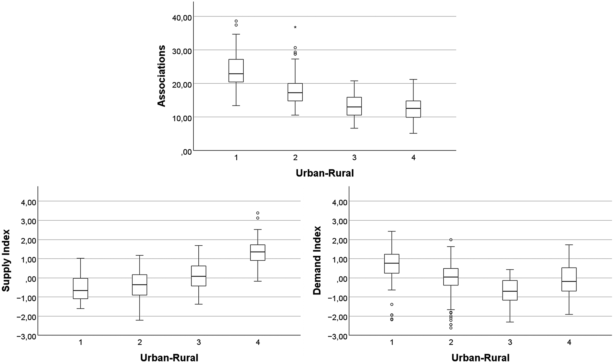
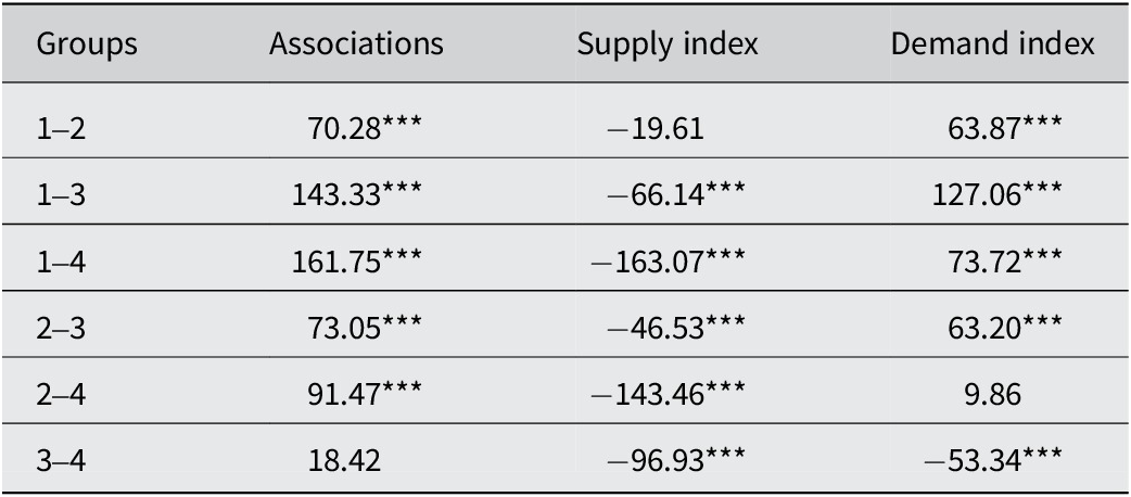
Figure 2 indicate that there are bound to be differences between municipalities per category in the urban–rural continuum. Indeed, as shown in Figure 3, SPAs and RHAs host more TSAs per population than RCAs and urban areas. These differences are statistically significant as verified by the Kruskal–Wallis test (Table 2). The socio-economic rationale behind the result is tied to poor performance in the supply and demand indices (Figure 3). Indeed, as verified by the Kruskal–Wallis test (Table 2), SPAs and RHAs perform in a similar manner: both have low supply but high demand index scores. Contrarily, while urban areas have similar demand index scores as RHAs, they have, on average, the highest supply index scores. Likewise, while RCAs have relatively low supply index scores, their demand index scores are the lowest among the urban–rural categories. To summarize, SPAs and RHAs perform the worst in both the supply and demand indices, but host more TSAs than RCAs and urban areas, which both do exceptionally well in one of the indices—urban areas have the highest supply while RCAs have the lowest demand index scores.
Performance of municipalities per urban–rural category based on the number of associations (per 1,000 inhabitants) and supply and demand indices. Urban–rural categories: 1 = sparsely populated rural areas (SPAs); 2 = rural heartland areas (RHAs); 3 = rural areas close to urban areas (RCAs); 4 = urban areas.

Fig. 3. Long description
A multi-panel figure containing three box plots. All plots share a horizontal X-axis labeled Urban-Rural with four categories: 1 (S P A s), 2 (R H A s), 3 (R C A s), and 4 (urban areas).
* Top Plot: Associations. The Y-axis ranges from ,00 to 40,00. Category 1 has the highest median (approximately 23) and highest range. The median decreases progressively through category 2 (median 17) and category 3 (median 13), remaining stable in category 4 (median 13). Outliers are present above the whiskers in categories 1 and 2.
* Bottom-Left Plot: Supply Index. The Y-axis ranges from -3,00 to 4,00. There is a clear upward trend from category 1 to 4. Category 1 has the lowest median (approximately -0,7), while category 4 has the highest median (approximately 1,4). Category 4 also shows two high outliers.
* Bottom-Right Plot: Demand Index. The Y-axis ranges from -3,00 to 4,00. Category 1 has the highest median (approximately 0,8). The median decreases in category 2 (approximately 0,1) and reaches its lowest point in category 3 (approximately -0,7), before rising slightly in category 4 (approximately -0,2). Categories 1 and 2 show several low outliers below the whiskers.
Results of the Kruskal–Wallis test

Table 2. Long description
The table consists of four columns: Groups, Associations, Supply index, and Demand index. There are six rows of pairwise comparisons between groups 1 through 4, where 1 represents sparsely populated rural areas, 2 represents rural heartland areas, 3 represents rural areas close to urban areas, and 4 represents urban areas.
* Row 1, Groups 1-2: Associations 70.28***, Supply index minus 19.61, Demand index 63.87***.
* Row 2, Groups 1-3: Associations 143.33***, Supply index minus 66.14***, Demand index 127.06***.
* Row 3, Groups 1-4: Associations 161.75***, Supply index minus 163.07***, Demand index 73.72***.
* Row 4, Groups 2-3: Associations 73.05***, Supply index minus 46.53***, Demand index 63.20***.
* Row 5, Groups 2-4: Associations 91.47***, Supply index minus 143.46***, Demand index 9.86.
* Row 6, Groups 3-4: Associations 18.42, Supply index minus 96.93***, Demand index minus 53.34***.
Triple asterisks indicate p-values significant at the 0.01 level adjusted by Bonferroni correction.
Notes: p-values significant at level: *** < 0.01 (p-values adjusted by Bonferroni correction for multiple tests). Dunn’s post hoc tests were used for the pairwise comparisons. Urban–rural categories: 1 = sparsely populated rural areas (SPAs); 2 = rural heartland areas (RHAs); 3 = rural areas close to urban areas (RCAs); 4 = Urban areas.
Regression approach
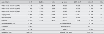
The linear regression results indicate that the prevalence of TSAs among Finnish municipalities is influenced significantly by the type of region, i.e., urban versus different rural typologies as well as by local socio-economic conditions, represented by the supply and the demand index (Table 3). SPAs have the highest coefficient value (+8.545; p < 0.001), indicating a much higher relative density of TSAs in comparison to urban areas (the reference group). RHAs also constitute a positive, but a more limited, impact on the number of TSAs per capita (+1.865; p < 0.001). RCAs, however, do not differ significantly from urban areas (+0.179; p = 0.580). The revealed pattern suggests that TSAs are, in relative terms, most common in the most isolated, least accessible, and least populated rural areas (SPAs), consistent with the notion that TSAs emerge as a “compensatory mechanism” to deliver a range of different services in regions where public and private channels are weaker.
Results of the linear regression analysis

Table 3. Long description
The table presents linear regression analysis results across eight columns: Associations, Coef., St. Err., t-value, p-value, 95% Conf. Interval (split into two columns), and Sig.
Main Associations:
* Urban-rural dummy 1 (S P A s): Coef. 8.545, St. Err. 1.025, t-value 8.34, p-value < 0.000, 95% CI [6.528, 10.562], Sig. ***.
* Urban-rural dummy 2 (R H A s): Coef. 1.865, St. Err. 0.476, t-value 3.92, p-value < 0.001, 95% CI [0.928, 2.802], Sig. ***.
* Urban-rural dummy 3 (R C A s): Coef. 0.179, St. Err. 0.323, t-value 0.55, p-value 0.580, 95% CI [-0.457, 0.814].
* Supply index: Coef. -0.966, St. Err. 0.368, t-value -2.63, p-value 0.009, 95% CI [-1.69, -0.242], Sig. ***.
* Demand index: Coef. 1.343, St. Err. 0.351, t-value 3.83, p-value < 0.001, 95% CI [0.652, 2.034], Sig. ***.
* Constant: Coef. 13.897, St. Err. 0.759, t-value 18.31, p-value < 0.001, 95% CI [12.403, 15.391], Sig. ***.
Model Statistics:
* Mean dependent var: 17.598; S D dependent var: 6.328.
* R-squared: 0.542; Number of obs: 292.
* F-test: 67.794; Prob > F: 0.000.
* Akaike crit. (A I C): 1688.870; Bayesian crit. (B I C): 1710.930.
Note: p-values significant at level *** < 0.01.
Note: p-values significant at level: *** < 0.01.
The above remark is further underlined by the results pertaining to the supply and demand indices. That is, from the point of view of socio-economic determinants, there is a negative connection between the supply index and number of TSAs per capita (−0.966; p = 0.009), which suggests that TSAs are less necessary in contexts with economic resources, human capital, and a strong presence of the public sector. In contrast, the demand index shows a marked positive connection to TSAs (+1.343; p < 0.001), indicating that a higher prevalence of social hardship (unemployment, poverty, and morbidity) is associated with a higher relative density of TSAs. These results reinforce the insight that TSAs emerge as social compensation devices, especially in rural regions.
The quality of the model is satisfactory with an R 2 of 0.542; the specification explains more than half of the variance in the dependent variable, a solid result for municipal-level data. The global F-test (67.794; p < 0.001) confirms the overall significance of the model. The information indices (AIC = 1688.870; BIC = 1710.930) provide additional supporting evidence of the goodness of fit of the selected model.
Conclusions
Summary of the main findings
Given the increasing role that TSAs are expected to play in maintaining and enhancing regional vitality (Makkonen & Kahila, Reference Makkonen and Kahila2021), their uneven geography can undermine the expected positive outcomes of such an “associational revolution” in third sector averse regions (Bryson et al., Reference Bryson, McGuiness and Ford2002; Salamon, Reference Salamon1999). Therefore, this paper set out to map the spatial spread of TSAs in Finland and to investigate the possible factors behind the potentially uneven geography of the Finnish third sector. To answer the first research question of this paper, the results indicate that TSAs tend to cluster geographically: in absolute numbers, the largest concentrations of TSAs can be found in (large) urban regions. However, when normalized per capita, the highest relative numbers of TSAs are found in SPAs, followed by RHAs. The result is partly explained by the normalization of the data. A certain number of common TSAs are active in most municipalities in Finland—but they vary significantly in size/membership. This raises the per capita TSAs figures in small rural municipalities.
In order to disentangle why rural municipalities are, in relative terms, more prone to host TSAs, two alternative explanations were explored: the supply and the demand side arguments. To do so, potential explanatory factors were arranged into two indices. The supply index combined variables indicating the potential availability of donative resources of households (proxied with educational levels), the private sector (firm turnover), and local government (municipal allowances). The demand index combined variables describing deprivation (including unemployment, poverty, and morbidity among the municipal populations), that is, a potential need for support that TSAs can meet. The results clearly indicate that the two rural area categories (SPAs and RHAs) that host the most TSAs per capita are the most socio-economically deprived municipalities in Finland, as indicated by their generally low supply but high demand index scores.
The urban–rural division between municipalities plays an important role in the geography of the third sector, as it is closely aligned with the socio-economic division between urban and rural municipalities in Finland. The result also coincides with previous studies showing a general division between the more socio-economically developed southern and western parts of Finland, compared to the regions with poorer socio-economic status, which are more commonly located in eastern and northern parts of the country (Makkonen & Inkinen, Reference Makkonen and Inkinen2015). Therefore, to answer the second research question of this paper, the high relative concentration of TSAs in Finland is connected to the high demand in socio-economically deprived regions rather than to affluent regions with high supply. Naturally, the results pertain to measurable items available at the municipal scale but cannot cover the full spectrum of potential reasons behind them. An important omission is the lack of an indicator proxying potential regional differences in willingness for volunteering and community spirit.
Implications
From a theoretical perspective, the results of this paper clearly support the demand-side explanation: higher demand is connected with higher per capita numbers of TSAs, as best exemplified by SPAs. Contrarily, the supply-side arguments do not seem to hold based on the data on Finnish municipalities. Rather, the case is the opposite: the association between the high economic standing of a municipality and the number of TSAs is negative. Indeed, even in the presence of the highest potential household, private sector, and local government donative resources, the number of TSAs per capita is the lowest in urban regions. In other words, deprivation seems to cause demand for TSAs, while high supply of private and public sector resources seems to coincide with low third sector activity. Thus, the results challenge assumptions that stronger economic resource bases necessarily foster denser third sector activity, while simultaneously lending support to interpretations connected to government failure theory and compensatory civic organization. The Finnish municipal data show that a combination of poor socio-economic performance in terms of both economic resources (supply) and population well-being (demand) is connected with high numbers of TSAs per population.
Evidently, the results raise questions of how to best explain the geography of the third sector. Our analysis cannot provide a definite answer, but traditional locational theories could enrich the existing theoretical discussions (Reiner & Wilson, Reference Reiner, Wilson, Blum, Funck, Kowalski, Kuklinksi, Rothengatter and von Thadden2007). Drawing from the seminal work by Lösch (Reference Lösch1954), we can posit that the private sector strives to expand profits by maximizing consumer access and minimizing transportation costs. At the same time, due to economic austerity, the public sector has been struggling to minimize the costs of service provision. Instead, the third sector operates to maximize access to community benefits. In other words, TSAs can be expected to emerge to fill in gaps where private and public sector actors do not operate. Similarly, the third sector can be expected to expand in two-dimensional space until they meet competition, i.e., a neighboring TSA. Since many of the services and activities provided by the third sector are consumed or enjoyed on site (e.g., sports, hobbies, social affairs, and health associations), it is sensible that also rural locations with a minimum sufficient population base requiring them will have their own TSAs despite them very likely being smaller in size compared to the ones in urban locations. Thus, different types of TSAs might be organized as a theoretical hexagonal grid type division based on the distance people are willing to travel to reach the various services and activities they provide.
Furthermore, since the locational decisions of TSAs do not seem to be strictly tied to economic resources or institutional surroundings, the behavioral locational theory (Hayter, Reference Hayter1997) could help to explain individual decisions to establish and run TSAs in rural regions. As in the case of rural entrepreneurship (Saarinen & Makkonen, Reference Saarinen, Makkonen, Leick, Gretzinger and Makkonen2022), the commitment to establish and run TSAs can be expected to stem from association activists’ levels of rural embeddedness, i.e., personal roots and social ties to a specific rural region (Milligan, Reference Milligan2007). These implications are potentially highly interesting for future research in and beyond the Finnish context.
From a practical perspective, the revealed mismatch between third sector demand and supply raises severe concerns for the future vitality of rural regions. If the public sector withdraws from rural regions—as we are now witnessing in Finland (Lehtonen et al., Reference Lehtonen, Makkonen, Vihinen, Hirvonen, Rautiainen and Voutilainen2025; Makkonen et al., Reference Makkonen, Lehtonen, Inkinen, Vihinen and Voutilainen2025)—on the positive side, there are proportionally abundant numbers of TSAs that could step in to alleviate the ensuing lack of various services (welfare, culture, leisure, etc.), facilitate local democracy, maintain communal participation, and help to secure vibrant community cultures. However, these rural regions, which are also undergoing depopulation and aging (Makkonen et al., Reference Makkonen, Inkinen and Rautiainen2022), on average, among the most poorly locally resourced regions, as shown by their low supply index scores. From the perspective of local societal challenges, this raises a question of whether the dwindling population base of rural regions can guarantee enough volunteers to participate in third sector activities and whether rural regions can financially support their “stock” of TSAs also in the future. The mismatch underlines the importance of sustained external funding from the state and/or the European Union, e.g., through Leader funding. Without such support, the combined impacts of public sector withdrawal and dwindling third sector activity would be detrimental to the vitality of rural regions.
Limitations
The conducted analyses have several limitations caused by the data and chosen methodology. These limitations, however, help pave the way for further research on the geography of the third sector.
First, the geography of the third sector, while also exhibiting multi-scalar connections ranging from the local to the global, is naturally tied to jurisdictions (Milligan, Reference Milligan2007; Woolvin et al., Reference Woolvin, Mills, Hardill and Rutherford2015). For example, in the Finnish case, TSAs operate in a wide range of activities, out of which service provision has only a secondary role (Matthies, Reference Matthies2007). In contexts where the service provision role of the third sector is more central, the result might differ from the ones presented here. As such, there are bound to be similarities but also distinct dissimilarities between the geography of the third sector across different countries (Salamon et al., Reference Salamon, Sokolowski and List2003). Therefore, there is a clear need for further comparative cross-country studies or meta-analysis based on the existing country-specific findings to shed light on these (dis-)similarities.
Second, the analyses are naturally limited by the cross-sectional nature of the data, focusing on a single point in time. Further studies should investigate time-series data to explore the geography of the third sector vis-á-vis policy reforms and demographic change to uncover how the third sector has evolved in regions. Unfortunately, such data are not readily available for the case of TSAs in Finnish municipalities but would require a backtracking approach by going through, year-by-year, the list of terminated TSAs (Pyykkönen et al., Reference Pyykkönen, Koski, Makkonen, Hirvonen and Kortelainen2026).
Third, the methods applied in this paper are descriptive and thus do not imply causality between the studied factors and the spatial location of TSAs. Therefore, more fine-tuned and elaborate statistical testing and spatial analyses are needed to fully understand the geography of the third sector. For example, while the distinction between urban and different types of rural areas already captures the territorial dimension in a structural way, one could run additional cluster and spatial autoregression analyses to uncover further spatial patterns underlying the data.
Fourthly, an obvious further step for analyzing the geography of the third sector in Finland would be to map TSAs individually per field of activity (culture, religious, etc.) as, e.g., in Marchesini da Costa (Reference Marchesini da Costa2016). This would, however, likely require using larger regional scales, as the numbers of specific types of TSAs are often zero or close to zero, particularly in the smallest municipalities, which hampers the data’s usability for statistical testing.
Fifthly, there are no readily available data on the size (membership or expenses) and activity of the Finnish TSAs, and, thus, testing whether, on average, certain types of regions host larger and more active TSAs than others remains outside the scope of this paper. Similarly, several likely factors behind the results, particularly potential regional variation in willingness to volunteer, remain at present quantitatively unobservable at the municipal level. These would be interesting questions for further analysis. Further studies should thus attempt to combine the available secondary statistical data with novel primary data sources, gathered, for example, via surveys.
Finally, as illustrated by Milligan and Fyfe (Reference Milligan and Fyfe2004) and MacIndoe and Oakley (Reference MacIndoe and Oakley2023), the physical location of a TSAs is not necessarily a true indicator of the area of its operations: they often cluster in urban centers but serve a population spread across a larger region rather than one specific municipality. Tackling this likely source of bias requires further research efforts.
Acknowledgements
We are grateful to Virpi Lemponen for her help in acquiring the data on Finnish third sector associations.
Author contributions
Conceptualization: T.M.; Data curation: T.M.; Formal analysis: T.M., L.E.; Methodology: L.E.; Visualization: S.R.; Writing—original draft: T.M; Writing—review & editing: L.E.
Funding statement
This work was supported by the Rural Policy Council from the Development Fund for Agriculture and Forestry of the Ministry of Agriculture and Forestry of Finland [Grant number: VN/5318/2024].
Competing interests
The authors declare that there is no conflict of interest.
Appendix
Descriptive statistics

Table A1. Long description
The table contains six columns: Indicator, N, Minimum, Maximum, Mean, and Std. Deviation.
* Education: N 293, Minimum 12.36, Maximum 59.30, Mean 24.19, Std. Deviation 6.53.
* Turnover: N 293, Minimum 59.09, Maximum 3271.02, Mean 429.45, Std. Deviation 414.13.
* Municipal allowances: N 293, Minimum 60.11, Maximum 819.63, Mean 236.87, Std. Deviation 110.65.
* Unemployment: N 293, Minimum 2.52, Maximum 18.27, Mean 10.31, Std. Deviation 2.92.
* Health morbidity: N 292, Minimum 71.28, Maximum 153.50, Mean 103.77, Std. Deviation 12.90.
* Income poverty: N 293, Minimum 4.96, Maximum 22.52, Mean 14.05, Std. Deviation 3.77.
* Urban-rural status: N 293, Minimum 1, Maximum 4, Mean 2.33, Std. Deviation 1.07.
* Associations: N 293, Minimum 5.18, Maximum 38.65, Mean 17.63, Std. Deviation 6.33.
Notes: For descriptions and data sources, see Table 1 in the main text.
Definition of urban–rural categories

Table A2. Long description
The table consists of two columns: Category and Definition.
* Urban areas: Defined as densely populated, relatively tightly connected built areas.
* Rural areas close to urban areas (R C A s): Located functionally and physically close to urban areas. Delimited based on potential accessibility and commuting patterns to urban areas, describing the wider functional working area.
* Rural heartland areas (R H A s): Strong primary production or relatively densely populated rural areas with diverse activities. Located far from large urban centers, characterized by medium-sized population centers and villages. Land use is intensive and dominated by agriculture.
* Sparsely populated rural areas (S P A s): Areas with minimal local economic structure and sparse populations. Located far from urban areas with fragmented settlement structures. The most common land use categories are forest or wetland.
Number of third sector associations per population: comparison of means by urban–rural type

Table A3. Long description
The table consists of three columns: Urban-rural type, Mean, and Std. Deviation.
* Sparsely populated rural areas (S P As): Mean 24.07, Std. Deviation 5.53.
* Rural heartland areas (R H As): Mean 18.18, Std. Deviation 4.79.
* Rural areas close to urban areas (R C As): Mean 13.42, Std. Deviation 3.57.
* Urban areas: Mean 12.39, Std. Deviation 3.13.
The data shows a downward trend where the mean number of associations decreases as the area type becomes more urbanized.



 Open access

