





Introduction
In ecology and in agricultural research, many traits are recorded through visual inspections in the form of ordinal scores or ratings. Often, these scores have an underlying percentage scale. Examples include soil erosion, plant canopy cover, plant vigour, plant lodging, herbicide efficiency and fungal leaf disease severity (Figure 1). The analysis of disease scoring data can provide insights relevant to integrated pest management. For example, it can help to enhance the understanding of spatial and temporal occurrences of diseases and their impact on yield losses (Laidig et al., Reference Laidig, Feike, Hadasch, Rentel, Klocke, Miedaner and Piepho2021a; Laidig et al., Reference Laidig, Feike, Klocke, Macholdt, Miedaner, Rentel and Piepho2021b; Laidig et al., Reference Laidig, Feike, Klocke, Macholdt, Miedaner, Rentel and Piepho2022; Willocquet et al., Reference Willocquet, Meza, Dumont, Klocke, Feike, Kersebaum, Meriggi, Rossi, Ficke, Djurle and Savary2021). To maximize accuracy, disease severity could in principle be assessed directly as exact percentages. However, it has been reported that it is faster to assess ordinal scores as compared to percentages (Hartung and Piepho, Reference Hartung and Piepho2007).
Example of an ordinal rating scale with an underlying percentage scale for disease ratings. Each ordinal score represents a defined range of percentages. Thresholds are the limits that indicate the transition to a new score. For this scale, there are five thresholds and the point score of zero.

Modelling plain ordinal scores is challenging. The data consist of ordered categories, represented by the ordinal scores. The differences between them cannot be interpreted quantitatively (Figure 1, column 3). Therefore, the means of such data have no biological meaning. Furthermore, the assumptions of normality and homogeneous variance of residuals are also not expected to hold. Since these assumptions are prerequisites for easy-to-handle standard methods such as analysis of variance (ANOVA), alternative methods are needed.
It is important to ensure that the chosen method for analysing a dataset fits the data type. The common randomization structures used in agricultural research trials can easily be accounted for in an ANOVA, the default method. However, if the collected data are ordinal scores, ANOVA assumptions are violated. This can result in inaccurate findings, e.g., regarding the ranking of the best performing variety (Onofri et al., Reference Onofri, Piepho and Kozak2019). One alternative for modelling ordinal data is using nonparametric methods. These do not assume a specific distribution, and multiple options are available. For example, one can test for relative marginal effects or use Wald-type statistics (Brunner et al., Reference Brunner, Bathke and Konietschke2018; Shah and Madden, Reference Shah and Madden2004). However, these methods also have assumptions and prerequisites that the data must meet. Furthermore, the results can be difficult to interpret, and the accuracy decreases as the number of regressors increases (Härdle et al., Reference Härdle, Müller, Sperlich and Werwatz2004). They are also often less efficient, requiring a larger sample size to obtain significant results (Luepsen, Reference Luepsen2024).
Alternatively, a parametric type of model, i.e., a multinomial ordinal model, could be used. In the current paper, it will be referred to as the ordinal threshold model (Hartung and Piepho, Reference Hartung and Piepho2005; McCullagh, Reference McCullagh1980). The threshold model is most suitable for ordinal scoring data encompassing multiple scorings per plot (Schumacher and Thöni, Reference Schumacher and Thöni1990). It assumes that an unobservable (latent) random variable underlies the observed scores, and that this variable is normally or logistically distributed (Piepho, Reference Piepho1998). This latent scale can be divided into as many intervals as there are score categories. On the latent scale, a linear model is assumed. The interval limits (thresholds) on the latent scale define the transition between ordinal categories (Figure 1). These limits are parameters to be estimated in addition to design and treatment effects in the linear predictor of the threshold model.
The ordinal rating scheme addressed here is based on an observable percentage scale, and the thresholds are already known (Figure 1). These data can be considered interval-censored on the underlying continuous percentage scale (Onofri et al., Reference Onofri, Piepho and Kozak2019). As such, there is a close connection with models used in survival analysis and time-to-event data (Bogaerts et al., Reference Bogaerts, Komárek and Lesaffre2017). Modelling solely by the classical threshold model neglects the information that is indeed available on the underlying percentage scale. Additionally including the known percentage thresholds in the model is computationally advantageous, since fewer parameters need to be estimated than in the classical threshold model. Moreover, the data differ from purely ordinal data in that the lowest scoring class corresponds to a single point on the underlying percentage scale (i.e., a lower bound of zero) (Figure 1). This difference is important because transformations that work with data on the percentage scale, such as logit transformations, do not permit exact zeros. It is desirable to account for the specific features of ordinal scores, that result from rating scales. Accounting for them allows us to use all available information. Therefore, the current work is inspired by the classical threshold model and develops an approach for analysing ordinal data with an underlying percentage scale.
Material and methods
A method for modelling data is proposed that considers both ordinal scorings with an underlying percentage scale and a separate class for 0% disease severity. This approach is described using an example from on-farm trials.
Example data
The data used originates from on-farm trials in grapevines (Appendix B). The trials were conducted in 2021 and 2022 at nine locations (Table S1). Eight different treatments (Table S2) were tested for their effect on powdery mildew (Erysiphe necator) and downy mildew (Plasmopara viticola). The treatments to be tested were applied to adjacent rows in vineyards. The vineyards were otherwise managed according to customary practices, which is considered as standard treatment. Except for the standard, each treatment existed once in each environment (Figure S1). An environment was defined as a location-year combination. In the on-farm trials, one grapevine row constituted one plot. The treatments were allocated to plots, ensuring optimal suitability for the farmer. The data were collected from the treated plots and the two adjacent standard plots. The trial design was unbalanced, as not all treatments were present or replicated in every environment (Tables S3 and S4). If a treatment was tested over two years, it was applied to the same plot in both years, because an adjustment of the vine to the individual treatment was expected. The data encompass two traits: (I) leaf and (II) fruit infestation scores. Note that infestation by both powdery and downy mildew was assessed in one joint trait. A scoring system with seven ordinal categories was used (Figure 1). 100 scores were collected per plot. Each score was obtained by evaluating a randomly chosen leaf or grape within the plot. The dataset contains scorings from one evaluation at one time point.
The hurdle model for scoring data
Our model targets scoring data with an underlying continuous percentage scale for disease severity bounded inside the range from ≥0% to ≤100%. The percentages were modelled using a parametric distribution, i.e., the Johnson S B distribution (Piepho and McCulloch, Reference Piepho and McCulloch2004). If applied to our data, this distribution assumes that logit-transformed percentages follow a normal distribution (Johnson, Reference Johnson1949), as discussed in more detail below. This was user-friendly to implement.
One specific challenge posed by cases with a disease severity of exactly 0% (scoring class ‘1’) is that they are not covered by the Johnson S B distribution or other distributions, such as the Beta distribution (Irvine et al., Reference Irvine, Rodhouse and Keren2016). The current approach specifically considers this feature using a two-part model. In the first part, a hurdle component is employed, with the 0% disease severity as the hurdle to be passed (Min and Agresti, Reference Min and Agresti2005; Ogutu et al., Reference Ogutu, Piepho, Reid, Rainy, Kruska, Worden, Nyabenge and Hobbs2010). In this first step, a binary random variable determines whether the hurdle is passed or not, corresponding to the presence or absence of disease. This enables the model to accommodate data with an excess of zeros. In the second step, if the hurdle of 0% disease severity is passed, the disease severity is modelled using a distribution for percentages >0%. Finally, the two components were integrated into a joint model.
Zooming in, the first step models the presence or absence of disease using a binary distribution. This is achieved by using the ordinal score of either $k = 1$
or
$k = 1$
or $k \gt 1$
, where
$k \gt 1$
, where $k = 1$
indicates absence of the disease (0% disease severity), and
$k = 1$
indicates absence of the disease (0% disease severity), and $k \gt 1$
indicates presence of the disease (>0% disease severity). This binary-distributed component of the hurdle model is subsequently referred to as INCIDENCE. It models the probability of the event
$k \gt 1$
indicates presence of the disease (>0% disease severity). This binary-distributed component of the hurdle model is subsequently referred to as INCIDENCE. It models the probability of the event $k = 1$
, i.e. 0% disease severity, the proportion of healthy plants. Disease incidence is defined as the proportion of diseased plants (Madden et al., Reference Madden, Hughes and van den Bosch2007), which in our case is essentially identical with the probability that k > 1.
$k = 1$
, i.e. 0% disease severity, the proportion of healthy plants. Disease incidence is defined as the proportion of diseased plants (Madden et al., Reference Madden, Hughes and van den Bosch2007), which in our case is essentially identical with the probability that k > 1.
The second model step considers only scores $k \gt 1$
, implying that the
$k \gt 1$
, implying that the $k = 1$
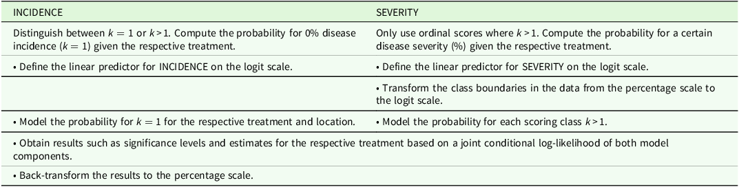
hurdle is passed. A multinomial distribution is then fitted to the frequencies of the corresponding ordinal categories. This second model component is referred to as SEVERITY. Note that, in epidemiology, disease severity is defined as the area of infected plant tissue (Madden et al., Reference Madden, Hughes and van den Bosch2007). Both components could be implemented as separate models. However, both model components were fitted in a joint analysis. An overview of the individual steps is given in Table 1.
$k = 1$
hurdle is passed. A multinomial distribution is then fitted to the frequencies of the corresponding ordinal categories. This second model component is referred to as SEVERITY. Note that, in epidemiology, disease severity is defined as the area of infected plant tissue (Madden et al., Reference Madden, Hughes and van den Bosch2007). Both components could be implemented as separate models. However, both model components were fitted in a joint analysis. An overview of the individual steps is given in Table 1.
Overview of the steps for analysing the data with the hurdle model, including the binary part (INCIDENCE) and the continuous part (SEVERITY). The linear predictor is defined on the logit scale, which ranges from −∞ to ∞. On this scale, terms combine additively. The probability is then obtained by applying the inverse logit
 $k = 1 \ldots K$
is the respective scoring class, with
$k = 1 \ldots K$
is the respective scoring class, with $K$
scoring classes.
$K$
scoring classes.
The model is described for a two-way classification of treatments and environments. Note that environments may correspond to combinations of years and locations. The data have $K = 7$
scoring classes
$K = 7$
scoring classes $k\;\left( {k = 1,{\rm{\;}} \ldots, {\rm{\;}}K} \right)$
. The analysis is conducted in SAS (SAS Institute Inc., 2024) using PROC NLMIXED. We evaluated each trait-year combination individually. Thus, four test datasets were available for developing the methodology.
$k\;\left( {k = 1,{\rm{\;}} \ldots, {\rm{\;}}K} \right)$
. The analysis is conducted in SAS (SAS Institute Inc., 2024) using PROC NLMIXED. We evaluated each trait-year combination individually. Thus, four test datasets were available for developing the methodology.
Statistical model for the two hurdle components
In the binary part, i.e., the INCIDENCE model component, the probability ${p_{ij}}$
, that an observed score for the i-th location and the j-th treatment equals
${p_{ij}}$
, that an observed score for the i-th location and the j-th treatment equals $k = 1$
, is estimated. For this purpose, a generalized linear mixed model is used with the linear predictor one
$k = 1$
, is estimated. For this purpose, a generalized linear mixed model is used with the linear predictor one $\left( {{\eta _{ij1}}} \right)$
and a logit link. The linear predictor for this model component is
$\left( {{\eta _{ij1}}} \right)$
and a logit link. The linear predictor for this model component is
 $${\eta _{ij1}} = {\mu _1} + {\rm{\;}}{l_{i1}} + {\rm{\;}}{t_{j1}}{\rm{\;}} + {\left( {lt} \right)_{ij1}}$$
where ${\eta _{ij1}}$
is the expected value, or mean value of the j-th treatment at the i-th environment, on the logit scale,
${\eta _{ij1}}$
is the expected value, or mean value of the j-th treatment at the i-th environment, on the logit scale, ${\mu _1}$
is the intercept,
${\mu _1}$
is the intercept, ${l_{i1}}$
is the fixed effect of environment i,
${l_{i1}}$
is the fixed effect of environment i, ${t_{j1}}$
is the fixed effect of treatment j, and
${t_{j1}}$
is the fixed effect of treatment j, and ${\left( {lt} \right)_{ij1}}$
is the random treatment-environment interaction (Piepho and Williams, Reference Piepho and Williams2024).
${\left( {lt} \right)_{ij1}}$
is the random treatment-environment interaction (Piepho and Williams, Reference Piepho and Williams2024).
Since this model would be overparametrized, a sum-to-zero restriction is implemented, so that the environment and treatment main effects both sum to zero. To implement this, dummy variables for the levels of both factors are added. An example dataset with further explanation is available in the supplementary material (Comment S1). In the binary part, the probability of score $k = 1$
, namely the probability of finding no disease at the respective environment and treatment, is obtained with the inverse logit of
$k = 1$
, namely the probability of finding no disease at the respective environment and treatment, is obtained with the inverse logit of ${\eta _{ij1}}$
as
${\eta _{ij1}}$
as
 $$\;{p_{ij}} = {1 \over {1 + \;ex{p^{ - {\eta _{ij1}}}}}}$$
Note that the disease incidence probability is given by $1 - {p_{ij}}$
. For the second model component, SEVERITY, only data of
$1 - {p_{ij}}$
. For the second model component, SEVERITY, only data of $k \gt 1$
is considered. The first step is to define its linear predictor
$k \gt 1$
is considered. The first step is to define its linear predictor $\left( {{\eta _{ij2}}} \right)$
. While different approaches can be applied to form a joint model, as a first option, two linear predictors with two full sets of parameters are assumed. In this case, the linear predictor for SEVERITY is given by
$\left( {{\eta _{ij2}}} \right)$
. While different approaches can be applied to form a joint model, as a first option, two linear predictors with two full sets of parameters are assumed. In this case, the linear predictor for SEVERITY is given by
 $${\eta _{ij2}} = {\mu _2} + {\rm{\;}}{l_{i2}} + {\rm{\;}}{t_{j2}}{\rm{\;}} + {\left( {lt} \right)_{ij2}}$$
For the case of two separate linear predictors for INCIDENCE and for SEVERITY, two individual parameters for the treatment $ \times $
environment effects’ variance are used. Therefore, a covariance (
$ \times $
environment effects’ variance are used. Therefore, a covariance ( $\sigma _{lt\left( {1,2} \right)}$
) between the two treatment
$\sigma _{lt\left( {1,2} \right)}$
) between the two treatment $ \times $
environment effects of the following form is also assumed:
$ \times $
environment effects of the following form is also assumed:

with $BVN$
denoting the bivariate normal distribution. The variances of
$BVN$
denoting the bivariate normal distribution. The variances of ${\left( {lt} \right)_{ij1}}$
and
${\left( {lt} \right)_{ij1}}$
and ${\left( {lt} \right)_{ij2}}$
are found on the diagonal and the covariance
${\left( {lt} \right)_{ij2}}$
are found on the diagonal and the covariance $\sigma_{lt\left(1,2\right)}$
is on the off-diagonal. The covariance was parameterized as follows:
$\sigma_{lt\left(1,2\right)}$
is on the off-diagonal. The covariance was parameterized as follows:
 $${\sigma _{lt\left( {1,2} \right)}} = {\rho _{lt}} \times \sqrt {{\sigma _{lt\left( 1 \right)}} \times {\sigma _{lt\left( 2 \right)}}} $$
where ${\rho _{lt}}$
is the correlation of the interactions
${\rho _{lt}}$
is the correlation of the interactions $(l{t)_{ij1}}$
and
$(l{t)_{ij1}}$
and $(l{t)_{ij2}}$
. In order to facilitate convergence, the correlation was parameterized according to the inverse Fisher’s z-transformation (Sokal and Rohlf, Reference Sokal and Rohlf2012) with
$(l{t)_{ij2}}$
. In order to facilitate convergence, the correlation was parameterized according to the inverse Fisher’s z-transformation (Sokal and Rohlf, Reference Sokal and Rohlf2012) with
 $${\rho _{lt}} = {{{{\exp }^{2 \times {\zeta _{lt}}}} - 1} \over {{{\exp }^{2 \times {\zeta _{lt}}}} + 1}}$$
where ${{\rm{\zeta }}_{lt}}$
is a parameter to be estimated. Similarly, the two variances were parameterized as
${{\rm{\zeta }}_{lt}}$
is a parameter to be estimated. Similarly, the two variances were parameterized as $\sigma _{lt\left( 1 \right)}^2 = {e^{{\omega _{lt1}}}}$
and
$\sigma _{lt\left( 1 \right)}^2 = {e^{{\omega _{lt1}}}}$
and $\sigma _{lt\left( 2 \right)}^2 = {e^{{\omega _{lt2}}}}$
, where
$\sigma _{lt\left( 2 \right)}^2 = {e^{{\omega _{lt2}}}}$
, where ${\omega _{lt1}}$
and
${\omega _{lt1}}$
and ${\omega _{lt2}}$
are the respective logarithms of the variances. This facilitates model fitting and obtaining a Hessian matrix that is positive definite.
${\omega _{lt2}}$
are the respective logarithms of the variances. This facilitates model fitting and obtaining a Hessian matrix that is positive definite.
After choosing the linear predictor for SEVERITY, the probability ${q_{{{ijk}}}}$
is modelled for the k-th score under a multinomial distribution. For this purpose, the thresholds
${q_{{{ijk}}}}$
is modelled for the k-th score under a multinomial distribution. For this purpose, the thresholds ${c_k}$
that define the shift to a new score are used. The percentage thresholds
${c_k}$
that define the shift to a new score are used. The percentage thresholds ${c_k}$
are expressed as a fraction, e.g. 5% becomes 0.05. As preliminary step,
${c_k}$
are expressed as a fraction, e.g. 5% becomes 0.05. As preliminary step, ${c_k}$
are logit transformed to obtain the thresholds
${c_k}$
are logit transformed to obtain the thresholds ${\theta _k}$ $\left( {k = 2,{\rm{\;}} \ldots, {\rm{\;}}K - 1} \right)$
on the linear predictor scale with
$\left( {k = 2,{\rm{\;}} \ldots, {\rm{\;}}K - 1} \right)$
on the linear predictor scale with
 $${\theta _k} = log\left( {\;{{{c_k}} \over {\;1 - {c_k}}}} \right)$$
According to the theory for the Johnson S
B
distribution (Johnson, Reference Johnson1949), the thresholds ${\theta _k}$
can be considered quantiles of the normal distribution. This is convenient because standard linear models can now be applied (Piepho and Kalka, Reference Piepho and Kalka2003), and the probability
${\theta _k}$
can be considered quantiles of the normal distribution. This is convenient because standard linear models can now be applied (Piepho and Kalka, Reference Piepho and Kalka2003), and the probability ${q_{{{ijk}}}}$
of observing a specific score
${q_{{{ijk}}}}$
of observing a specific score $k$
was be calculated according to the threshold model as
$k$
was be calculated according to the threshold model as
 $${q_{{{ijk}}}} = {\it{\Phi}} \left( {{{{{\theta _k} - \;{\eta _{ij2}}} } \over \sigma }} \right)\; - {\it{\Phi}} \left( {{{{{\theta _{k - 1}} - \;{\eta _{ij2}}} } \over \sigma }} \right)\;$$
where ${\it{\Phi}} \left( . \right)$
is the cumulative distribution function of the standard normal (Piepho and Kalka, Reference Piepho and Kalka2003; Hartung and Piepho, Reference Hartung and Piepho2005),
${\it{\Phi}} \left( . \right)$
is the cumulative distribution function of the standard normal (Piepho and Kalka, Reference Piepho and Kalka2003; Hartung and Piepho, Reference Hartung and Piepho2005), $\sigma $
is the error standard deviation that here pertains to the individual fruit or leaf that was evaluated.
$\sigma $
is the error standard deviation that here pertains to the individual fruit or leaf that was evaluated. $\sigma $
is an additional parameter that is estimated. This formula for the multinomial probability determines, based on the probability mass function for discrete random variables, ‘the area under the normal density in the intervals bordered by the threshold values (Piepho and Kalka, Reference Piepho and Kalka2003). This model fits two sets of independent parameters, one for
$\sigma $
is an additional parameter that is estimated. This formula for the multinomial probability determines, based on the probability mass function for discrete random variables, ‘the area under the normal density in the intervals bordered by the threshold values (Piepho and Kalka, Reference Piepho and Kalka2003). This model fits two sets of independent parameters, one for ${\eta _{ij1}}$
and one for
${\eta _{ij1}}$
and one for ${\eta _{ij2}}$
.
${\eta _{ij2}}$
.
As a second option, alternatively to using two separate linear predictors, ${\eta _{ij2}}$
can be replaced by a linear function of
${\eta _{ij2}}$
can be replaced by a linear function of ${\eta _{ij1}}$
with
${\eta _{ij1}}$
with
 $${\eta _{ij2}} = {v_0} + {v_1}{\eta _{ij1}}$$
where ${v_0}$
and
${v_0}$
and ${v_1}$
are scalar parameters. In this case, the only estimated parameters are parameters of
${v_1}$
are scalar parameters. In this case, the only estimated parameters are parameters of ${\eta _{ij1}},$
as well as
${\eta _{ij1}},$
as well as ${v_0}$
and
${v_0}$
and ${v_1}$
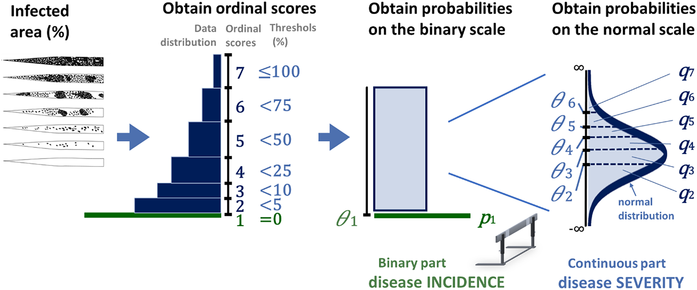
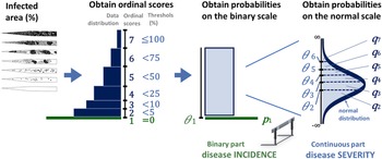
. This reduced model is computationally more efficient and more parsimonious. A likelihood ratio test (Rao, Reference Rao1973) was used to evaluate which of the two alternatives to choose. It should be noted that the test places the correlation parameter at the boundary of the parameter space and hence the test must be regarded as approximate (Self and Liang, Reference Self and Liang1987). The hurdle model with separate linear predictors was regarded as the full model, while the one with combined linear predictors was the reduced model. The null hypothesis assumed that there was no improvement of the full model compared to the reduced model. The workflow of the described model is illustrated in Figure 2.
${v_1}$
. This reduced model is computationally more efficient and more parsimonious. A likelihood ratio test (Rao, Reference Rao1973) was used to evaluate which of the two alternatives to choose. It should be noted that the test places the correlation parameter at the boundary of the parameter space and hence the test must be regarded as approximate (Self and Liang, Reference Self and Liang1987). The hurdle model with separate linear predictors was regarded as the full model, while the one with combined linear predictors was the reduced model. The null hypothesis assumed that there was no improvement of the full model compared to the reduced model. The workflow of the described model is illustrated in Figure 2.
Illustration of the hurdle model, starting from the left with disease scorings, continuing with the binary model component (INCIDENCE), and the continuous component (SEVERITY). A scoring scheme with seven classes $\left( {k = 1,{\rm{\;}} \ldots, {\rm{\;}}7} \right)$
was used. INCIDENCE’s probability of
$\left( {k = 1,{\rm{\;}} \ldots, {\rm{\;}}7} \right)$
was used. INCIDENCE’s probability of $k = 1$
, of being disease free, is
$k = 1$
, of being disease free, is ${p_{\rm{1}}}$
. The probabilities for disease severity for
${p_{\rm{1}}}$
. The probabilities for disease severity for $k = 2,{\rm{\;}} \ldots, {\rm{\;}}7$
are
$k = 2,{\rm{\;}} \ldots, {\rm{\;}}7$
are ${q_2}$
to
${q_2}$
to ${q_{\rm{7}}}.$
These are provided by the area under the normal density function and are separated by the thresholds
${q_{\rm{7}}}.$
These are provided by the area under the normal density function and are separated by the thresholds ${\theta _2}$
to
${\theta _2}$
to ${\theta _6}$
(Piepho and Kalka, Reference Piepho and Kalka2003).
${\theta _6}$
(Piepho and Kalka, Reference Piepho and Kalka2003).
Achieving convergence and improving model fit
Convergence was achieved with suitable starting values for the parameters. Starting values obtained from simpler models often failed to aid convergence, for example, starting values from the threshold model fitted in PROC GLIMMIX with cumulative probits. Instead, suitable starting values were identified by inspecting the estimated covariance matrix of the parameters. Patterns of singularity problems were examined under different initializations, which led to stable convergence. In addition, we used different optimization methods available through the ‘TECHNIQUE=’ option of PROC NLMIXED (SAS Institute Inc., 2024). Furthermore, reiterating with all previously estimated parameters as initial values did not usually improve model fit. Reiterating with the converged fixed-effect estimates while retaining the original starting values for the variance (0.9) and covariance (0.1) generally improved the model fit.
The joint log-likelihood of the two hurdle model components
Since the hurdle model is a two-part model, it also yields a two-part result. Estimates for INCIDENCE inform about disease incidence, while the estimations resulting from SEVERITY inform about disease severity. Originally, the two individual components INCIDENCE and SEVERITY each have their own likelihoods: one for the binary component for whether plants are infected, and another for the SEVERITY component describing the degree of disease infestation. A joint log-likelihood was derived from these individual likelihoods.
The conditional log-likelihood for a binary distributed trait, with ${n_{ij}}$
observations for the i-th environment and j-th treatment, is then given by
${n_{ij}}$
observations for the i-th environment and j-th treatment, is then given by
 $$\log L = {u_{ij1}}\log \left( {{p_{ij1}}} \right) + \left( {{n_{ij}} - {u_{ij1}}} \right)\log \left( {1 - {p_{ij1}}} \right)$$
where ${u_{ij1}}$
is the number of events and
${u_{ij1}}$
is the number of events and $({n_{ij}} - {u_{ij1}})$
the number of non-events and
$({n_{ij}} - {u_{ij1}})$
the number of non-events and ${p_{ij1}}$
is the probability for an event. In this case, the event is that the plants remain uninfected. It is symbolized by a rating score of
${p_{ij1}}$
is the probability for an event. In this case, the event is that the plants remain uninfected. It is symbolized by a rating score of $k = 1$
. Thus, for a binary model, the contribution to the conditional log-likelihood for the probability
$k = 1$
. Thus, for a binary model, the contribution to the conditional log-likelihood for the probability $P\left( {k = 1} \right)$
is
$P\left( {k = 1} \right)$
is ${u_{ij1}}\log \left( {{p_{ij1}}} \right)$
and for
${u_{ij1}}\log \left( {{p_{ij1}}} \right)$
and for $P(k \gt 1)$
it is
$P(k \gt 1)$
it is $\left( {{n_{ij}} - {u_{ij1}}} \right)\log \left( {1 - {p_{ij1}}} \right)$
. Note that
$\left( {{n_{ij}} - {u_{ij1}}} \right)\log \left( {1 - {p_{ij1}}} \right)$
. Note that ${u_{ij1}}$
includes the index 1 for
${u_{ij1}}$
includes the index 1 for $k = 1$
, while
$k = 1$
, while ${n_{ij}}$
does not include an index for the rating class as it compromises all classes
${n_{ij}}$
does not include an index for the rating class as it compromises all classes $k \gt 1$
.
$k \gt 1$
.
In case plants are infected, considering scores of $k = 2, \ldots, K$
, the conditional log-likelihood is multinomial with
$k = 2, \ldots, K$
, the conditional log-likelihood is multinomial with
 $$\log L = \;{u_{ij2}}\log \left( {{q_{ij2}}} \right) + {u_{ij3}}\log \left( {{q_{ij3}}} \right) + \; \ldots \; + \;{u_{ijK}}\log \left( {{q_{ijK}}} \right)$$
Hence, the contribution to the conditional log-likelihood for $k \gt 1$
in the hurdle model, comprising both, INCIDENCE and SEVERITY is
$k \gt 1$
in the hurdle model, comprising both, INCIDENCE and SEVERITY is
 $$\!\!\!\!\!\!\!\!\!\!\!\!\!\!\!\!\!\!\!\!\!\!\!\!\!\!\!\!\!\!\!\!\!\!\!\!\!\!\!\!\!\!\!\!\!\!\!\!\!\!\!\!\!\!\!\!\!\!\!\!\!\!\!\!\!\!\!\!\!\!\!\log L = \;\left( {{n_{ij}} - {u_{ij1}}} \right)\log \left( {1 - {p_{ij1}}} \right) + $$
 $$\quad\quad\quad{u_{ij2}}\log \left( {{q_{ij2}}} \right) + {u_{ij3}}\log \left( {{q_{ij3}}} \right) + \; \ldots \; + \;{u_{ijK}}\log \left( {{q_{ijK}}} \right)$$
Therefore, the joint conditional log-likelihood is
 $$\!\!\!\!\!\!\!\!\!\!\!\!\!\!\!\!\!\!\!\!\!\!\!\!\!\!\!\!\!\!\!\!\!\!\!\log L = {u_{ij1}}\log \left( {{p_{ij1}}} \right) + \left( {{n_{ij}} - {u_{ij1}}} \right)\log \left( {1 - {p_{ij1}}} \right) + $$
 $$\quad\quad\;\; {u_{ij2}}\log \left( {{q_{ij2}}} \right) + {u_{ij3}}\log \left( {{q_{ij3}}} \right) + \; \ldots \; + \;{u_{ijK}}\log \left( {{q_{ijK}}} \right)$$
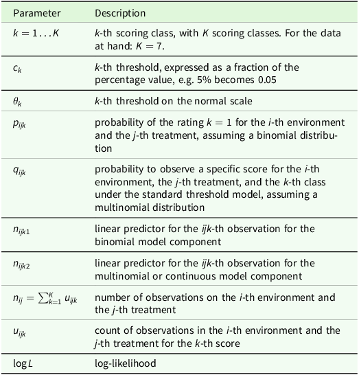
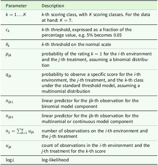
with the respective parameters described in Table 2. The marginal log-likelihood is obtained by integrating out the random effects using adaptive Gaussian quadrature (Pinheiro and Bates, Reference Pinheiro and Bates1995). The SAS code of the model is given in the supplementary material (SAS-Code S1).
Overview table for parameters and indexes
Interestingly, the joint conditional likelihood in Equation (13) can be re-written as a multinomial likelihood
 $$p_1^{{u_1}}{\left( {1 - {p_1}} \right)^{n - {u_1}}}q_2^{{u_2}}q_3^{{u_3}} \ldots q_K^{{u_K}} = p_1^{{u_1}}p_2^{{u_2}} \ldots p_K^{{u_K}}$$
where $p = \left( {1 - {p_1}} \right){q_K}$
for
$p = \left( {1 - {p_1}} \right){q_K}$
for $1 \lt k \le K$
. Note that
$1 \lt k \le K$
. Note that ${u_1} + {u_2} + \ldots + {u_K} = n$
,
${u_1} + {u_2} + \ldots + {u_K} = n$
, ${q_2} + {q_3} + \ldots + {q_K} = 1$
, and
${q_2} + {q_3} + \ldots + {q_K} = 1$
, and ${p_1} + {p_2} + \ldots + {p_K} = 1$
. To keep the notation simple, subscripts
${p_1} + {p_2} + \ldots + {p_K} = 1$
. To keep the notation simple, subscripts $i$
and
$i$
and $j$
for environments and treatments were omitted here. The multinomial nature of the hurdle model’s joint conditional log-likelihood is advantageous, because it enables the direct comparison with the threshold model.
$j$
for environments and treatments were omitted here. The multinomial nature of the hurdle model’s joint conditional log-likelihood is advantageous, because it enables the direct comparison with the threshold model.
Comparing the fit of the hurdle models and the threshold model
The suitability of all three models was compared: the hurdle model with joint linear predictors, the hurdle model with separate linear predictors, and the threshold model. The comparison metric was the Akaike Information Criterion (AIC). The prerequisites for using the AIC are met: All three methods use the same dataset and the maximum likelihood approach. In addition, as previously described, a LR test was conducted to compare the hurdle model with joint and separate linear predictors.
Treatment comparisons
Analogous to a standard ANOVA, treatment effects, Wald tests and P-values can be obtained. Significance tests were conducted for treatments and environments. P-values were estimated for the treatment and the environment effects. Furthermore, the model output provides effect estimates for all parameters in the linear predictor. Treatment means are obtained with
 $${\bar \eta _j} = \mu + \;{t_j} + {{\sum {{l_i}} } \over n}\;$$
where ${\bar \eta _j}$
is the j-th treatment mean on the logit scale and
${\bar \eta _j}$
is the j-th treatment mean on the logit scale and $n$
is the number of environments. For simplicity the index for the two individual linear predictors is not displayed. If joint linear predictors are used, the formula is applied only to
$n$
is the number of environments. For simplicity the index for the two individual linear predictors is not displayed. If joint linear predictors are used, the formula is applied only to ${\eta _{ij1}}$
. In the case of two separate linear predictors, the formula is applied independently to
${\eta _{ij1}}$
. In the case of two separate linear predictors, the formula is applied independently to ${\eta _{ij1}}$
and
${\eta _{ij1}}$
and ${\eta _{ij2}}$
. Note that the sum-to-zero parameterization,
${\eta _{ij2}}$
. Note that the sum-to-zero parameterization, $\sum {l_i} = 0$
, allows the general form of (15) to be simplified to
$\sum {l_i} = 0$
, allows the general form of (15) to be simplified to ${\bar \eta _j} = {\rm{\mu }} + {\rm{\;}}{t_j}$
. To obtain the treatment means on the original percentage scale, the treatment means obtained in (15) are back-transformed using the inverse logit function
${\bar \eta _j} = {\rm{\mu }} + {\rm{\;}}{t_j}$
. To obtain the treatment means on the original percentage scale, the treatment means obtained in (15) are back-transformed using the inverse logit function
 $${\mu _j} = {1 \over {1 + \;ex{p^{ - {{\bar \eta }_j}}}}}$$
where ${\mu _j}$
is the j-th treatment mean on the percentage scale. To obtain confidence limits (CL) on the percentage scale, the 95% CL of the treatment means on the logit scale were back-transformed, just as in (16). The global null hypothesis of no differences between treatments or environments was tested using a Wald test. This test was implemented using the contrast statement in SAS (SAS-Code S1). To obtain a letter display, pairwise differences were obtained for all treatment effects. The P-values were processed further in R (R Core Team, 2024) using the multcompLetters function of the multcompView package (Graves et al., Reference Graves, Piepho and Selzer2019). Disease incidence was estimated as the probability of an infection (1−p).
${\mu _j}$
is the j-th treatment mean on the percentage scale. To obtain confidence limits (CL) on the percentage scale, the 95% CL of the treatment means on the logit scale were back-transformed, just as in (16). The global null hypothesis of no differences between treatments or environments was tested using a Wald test. This test was implemented using the contrast statement in SAS (SAS-Code S1). To obtain a letter display, pairwise differences were obtained for all treatment effects. The P-values were processed further in R (R Core Team, 2024) using the multcompLetters function of the multcompView package (Graves et al., Reference Graves, Piepho and Selzer2019). Disease incidence was estimated as the probability of an infection (1−p).
Results
The Results section first presents a comparison between the hurdle models and the threshold model. Second, the results of the data analysed with the most suitable model, are presented: the hurdle model with separate linear predictors. Significance tests of the hurdle model with dependent linear predictors and results of the threshold model are provided in the supplementary material (Tables S7 and S8).
Model comparison
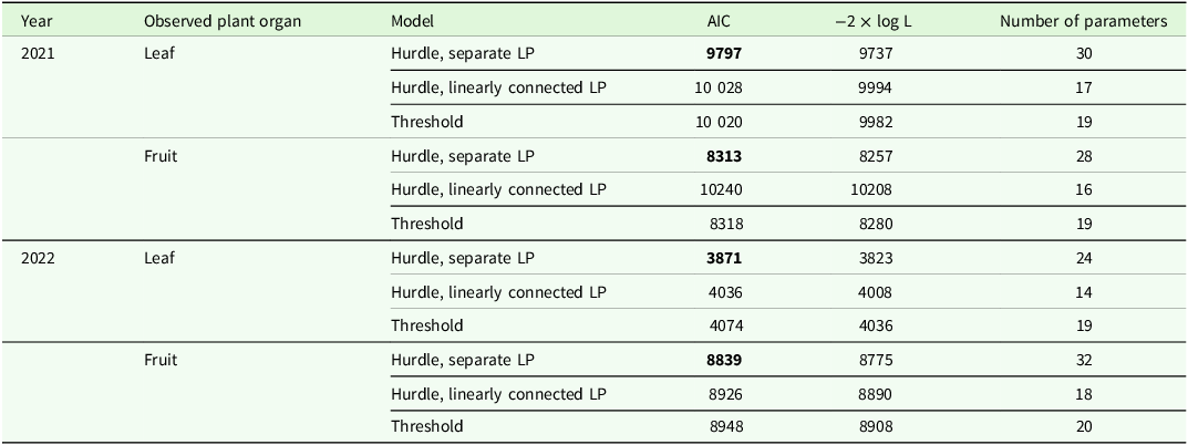
The three models were compared: i) the hurdle model with separate linear predictors, ii) the hurdle model with linearly connected linear predictors and iii) the threshold model. The results of the model comparison are shown in Table 3. According to the AIC, the hurdle model with two separate linear predictors is the most suitable for all datasets. However, depending on the dataset, different models perform second-best.
Comparing the hurdle model with separate linear predictors with the hurdle model with linearly connected linear predictors and the threshold model. Models were compared based on the Akaike Information Criterion (AIC). A smaller AIC indicates a better model fit. Each combination of the observed plant organ and year was evaluated as own dataset. Each dataset was evaluated with all three models. For better readability, the smallest AIC within each dataset is highlighted in bold
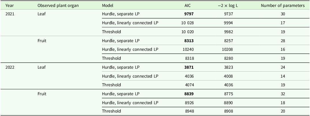
Log L = log-likelihood, LP = linear predictor.
To test whether the improvement of the hurdle model with separate linear predictors compared to the model with linearly connected linear predictors is significant, a LR test was performed (Rao, Reference Rao1973). The results are highly significant in all cases (P < 0.0001) (Table S6), indicating that the hurdle model with separate linear predictors performs significantly better than the hurdle model with joint linear predictors. This result is in line with the one presented in Table 3: the hurdle model with separate linear predictors shows the best fit.
Results of the fitted models
Significance levels of environment and treatment effects
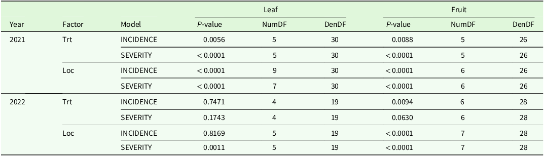
Tests for significance the hurdle model with separate linear predictors are displayed in Table 4. Results vary depending on the trait and respective year. Treatment effects for INCIDENCE are significant in three of the four cases, while treatment effects for SEVERITY are significant in two out of the four cases.
Results of significance tests for the hurdle model with independent linear predictors
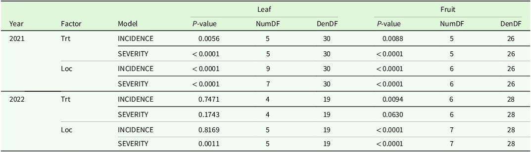
NumDF = numerator degrees of freedom, DenDF = denominator degrees of freedom, Trt = treatment effect, Loc = location effect, one location is one environment, INCIDENCE = result for the binomial part of the hurdle model, SEVERITY = result for the multinomial part of the hurdle model.
Performance of individual treatments
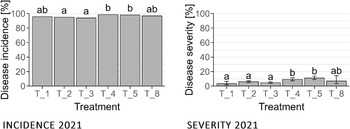
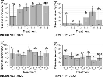
Figures 3 and 4 display the means of individual treatments on a percentage scale, as well as the letter display based on the pairwise differences in treatment effects. The plots for disease incidence show the probability of the evaluated unit (fruit or leaf) to be infected.
Mean mildew infestation [%] on leaves for data sets with a significant treatment effect. Treatments (T_1 to T_8) with the same letter are not significantly different. The error bar shows the 95% confidence limits. INCIDENCE = result of the first part of the hurdle model; Disease incidence = probability of being infected × 100%; SEVERITY = result of the second part of the hurdle model; Disease severity = area of infected plant tissue (in %).

Mean mildew infestation [%] on fruits for data sets showing a significant treatment effect. The error bar shows the 95% confidence limits. Treatments with at least one identical letter are not significantly different. INCIDENCE = result of the first part of the hurdle model; Disease incidence = probability of being infected × 100%; SEVERITY = result of the second part of the hurdle model; Disease severity = area of infected plant tissue (in %).

Confidence limits (CL) for means of disease incidence in 2021 reach from zero to 100 and are not displayed in Figure 3. The plot with CLs is shown in the supplementary material (Figure S2). The cause of the large standard errors and wide intervals for this trait in 2021 is that in one location all scores were above 0% disease severity.
There were only slight differences between the treatments for leaf evaluations in 2021. Fruit evaluations differed more. T_5 performed the worst in 2021. In 2022, T_3 and T_7 performed best.
Discussion
The hurdle model was initially developed for count data (Min and Agresti, Reference Min and Agresti2005). Among others it was employed to model species abundance in African savannas (Ogutu et al., Reference Ogutu, Piepho, Reid, Rainy, Kruska, Worden, Nyabenge and Hobbs2010) or to explore the microbiome (Qiao et al., Reference Qiao, Barnes, Tringe, Schachtman and Liu2023). It was also tested on ground coverage of trees and was found suitable for analysing percentage data with a zero-augmented Beta distribution (Irvine et al., Reference Irvine, Rodhouse and Keren2016). The hurdle model presented in this paper is designed to evaluate scoring data defined on an underlying percentage scale. This type of data is often used in ecological and agricultural research, such as in plant breeding and plant pathology.
Model comparison
In the grapevine example, the hurdle model with separate linear predictors was found superior to the threshold model. This finding aligns with the conclusion of Irvine et al. (Reference Irvine, Rodhouse and Keren2016) who tested multiple zero-inflated model options for ordinal responses. Note in passing that we use the common term zero-inflation here, which is usually meant to indicate that there are more zeros than expected under a simpler parametric model, even though strictly speaking our models are zero-augmented rather than zero-inflated in that the SEVERITY component comprises no zeros to begin with. Irvine et al. (Reference Irvine, Rodhouse and Keren2016) found that their ordinal beta hurdle model was superior to other models in terms of reduced uncertainty in posterior distributions. In a simulation study, Xu et al. (Reference Xu, Paterson, Turpin and Xu2015) compared standard parametric and nonparametric models, hurdle models, and zero-inflated models. While the standard models underestimated the probability of zeros, the hurdle and zero-inflated models displayed convincing performance with well controlled type one errors, higher power, better goodness-of-fit, and more accurate parameter estimation.
There are three main reasons why the hurdle model with separate linear predictors outperforms the threshold model. First, the hurdle model incorporates the available information about the underlying percentages, whereas the threshold model solely considers the ordinal scores. A drawback of the two-part model is that it considers a smaller sample size for the disease severity part, because the zeros are omitted (Lachenbruch, Reference Lachenbruch2002). Second, due to the (underlying) percentage scale, the data contains the point score of zero as lowest scoring class. Conversely, for the lowest scoring class, the threshold model estimates the range in which the lowest scorings fall on a latent scale. On the latent logit scale this ranges from $ - \infty $
to the lowest estimated threshold. Furthermore, exact zeros are also not considered by many popular distributions, such as in the Beta distribution and the Johnson S
B
distribution. For these distributions, an observed zero cannot be modelled as an exact zero but can only be approximated as a very small value. Rather than setting zero to a very small value, the hurdle model considers the zero individually in its binary part. This enables the model to accommodate data with an excess of score ‘1’ (=0% disease severity), e.g., originating from a population of healthy plants. Several authors have pointed out that hurdle models effectively handle excess zeros by modelling them separately Kheder and Yun (Reference Kheder and Yun2024), Naranammal and Krishna (Reference Naranammal and Krishna2024) and Asghar et al. (Reference Asghar, Ali and Shah2023), which is consistent with the present result. Third, the output of the hurdle model is user-friendly and easy to interpret. It provides individual estimates for the two model components, INCIDENCE and SEVERITY. The INCIDENCE component provides information about the probability of having completely healthy plants, while the SEVERITY component informs about the severity of an infection. This agrees with Irvine et al. (Reference Irvine, Rodhouse and Keren2016) who stated for their hurdle model that ‘striking differences’ were found in the conclusions that otherwise would not have been apparent.
$ - \infty $
to the lowest estimated threshold. Furthermore, exact zeros are also not considered by many popular distributions, such as in the Beta distribution and the Johnson S
B
distribution. For these distributions, an observed zero cannot be modelled as an exact zero but can only be approximated as a very small value. Rather than setting zero to a very small value, the hurdle model considers the zero individually in its binary part. This enables the model to accommodate data with an excess of score ‘1’ (=0% disease severity), e.g., originating from a population of healthy plants. Several authors have pointed out that hurdle models effectively handle excess zeros by modelling them separately Kheder and Yun (Reference Kheder and Yun2024), Naranammal and Krishna (Reference Naranammal and Krishna2024) and Asghar et al. (Reference Asghar, Ali and Shah2023), which is consistent with the present result. Third, the output of the hurdle model is user-friendly and easy to interpret. It provides individual estimates for the two model components, INCIDENCE and SEVERITY. The INCIDENCE component provides information about the probability of having completely healthy plants, while the SEVERITY component informs about the severity of an infection. This agrees with Irvine et al. (Reference Irvine, Rodhouse and Keren2016) who stated for their hurdle model that ‘striking differences’ were found in the conclusions that otherwise would not have been apparent.
Comparing the hurdle model with separate linear predictors and the one with linearly connected linear predictors, the hurdle model with connected linear predictors was expected to perform better, due to its computational efficiency. Contrary to expectations, assuming two connected linear predictors proved overly restrictive. It is worth the computational cost to estimate two separate sets of parameters. However, dependence is captured through a covariance structure.
The hurdle model described in the current paper is similar to another two-part model, namely the zero-inflated beta model (ZIB). The comparison has multiple facets. First, there are several options to account for zero inflation. Here, two linear predictors were utilized, one for the INCIDENCE and one for the SEVERITY component. By contrast, ZIB often incorporates just one extra parameter into the model to account for excess of zeros (Ospina and Ferrari, Reference Ospina and Ferrari2012). Second, for the SEVERITY part of the model, a Johnson S B distribution was used. It is easy to implement because it involves a logit transformation to normality (Hartung and Piepho, Reference Hartung and Piepho2005; Piepho and McCulloch, Reference Piepho and McCulloch2004). The Beta distribution is more frequently applied. It has a similar shape (Johnson et al., Reference Johnson, Kotz and Balakrishnan1994) and is certainly a viable alternative option (Ospina and Ferrari, Reference Ospina and Ferrari2012). Third, zero-inflated beta models usually handle continuously distributed data. The current hurdle model is developed for interval-censored data, and the scores’ probabilities are estimated using a multinomial distribution. As demonstrated by Irvine et al. (Reference Irvine, Rodhouse and Keren2016), the Beta distribution can also be fit to interval-censored percentage data.
Data
The described model is best suited for data encompassing scores of $k = 1$
and
$k = 1$
and $k \gt 1$
in all environments. When modelling
$k \gt 1$
in all environments. When modelling $P\left( {k = 1} \right)$
and environments with no scores of ‘1’ (all samples infected) exist, the estimated value of the linear predictor for the INCIDENCE component may get very low, approaching minus infinity on the logit scale. Transformed to the original percentage scale, the probability would approach 0%, causing inflated standard errors and yielding wide and unstable confidence limits. This was observed for environment L_2 in the dataset for leaf evaluations in 2021. In the same vein, Irvine et al. (Reference Irvine, Rodhouse and Keren2016, p. 636) reported that even though ‘the ordinal beta hurdle model outperformed other ordinal models in terms of lower uncertainty in posterior distributions, sample size and a very sparse distribution (e.g., rarity) could lead to estimation instability’. Options to circumvent this issue could be to evaluate a larger number of individuals within an experimental unit, a trial design with true replicates, a choice of environments and an evaluation period that enables a good differentiation and spread in disease severity. Furthermore, Bayesian models could be considered, as elaborated in the section ‘Software implementation’.
$P\left( {k = 1} \right)$
and environments with no scores of ‘1’ (all samples infected) exist, the estimated value of the linear predictor for the INCIDENCE component may get very low, approaching minus infinity on the logit scale. Transformed to the original percentage scale, the probability would approach 0%, causing inflated standard errors and yielding wide and unstable confidence limits. This was observed for environment L_2 in the dataset for leaf evaluations in 2021. In the same vein, Irvine et al. (Reference Irvine, Rodhouse and Keren2016, p. 636) reported that even though ‘the ordinal beta hurdle model outperformed other ordinal models in terms of lower uncertainty in posterior distributions, sample size and a very sparse distribution (e.g., rarity) could lead to estimation instability’. Options to circumvent this issue could be to evaluate a larger number of individuals within an experimental unit, a trial design with true replicates, a choice of environments and an evaluation period that enables a good differentiation and spread in disease severity. Furthermore, Bayesian models could be considered, as elaborated in the section ‘Software implementation’.
Based on the experience with the hurdle model described here, convergence was achieved when suitable starting values were provided. Furthermore, fitting the threshold model (McCullagh, Reference McCullagh1980) was facilitated by having multiple scorings per plot (Hartung and Piepho, Reference Hartung and Piepho2005; Thöni, Reference Thöni1985). The on-farm dataset contained 100 scorings per plot. Because the SEVERITY part of the hurdle model is based on the threshold model, having multiple scorings per plot will help to achieve convergence.
The proposed hurdle model uses interval-censored data, similar to the models used in survival analysis. Survival analysis concerns a continuous variable, typically time, that is interval-censored. This means that the observable unit becomes an interval and not an exact measurement, e.g. the survival time after an event (McCullagh and Nelder, Reference McCullagh and Nelder1989). The similarity in the data allows the methodology used for survival analysis to be applied to the interval-censored percentage data. Conversely, the hurdle model could be applied to time-to-event data. One example are data from germination and emergence assays (Onofri et al., Reference Onofri, Mesgaran and Ritz2022).
In theory, the data would not need to be interval-censored, as the exact percentage could be measured as a metric variable. However, collecting ordinal scores is thought to be more time-efficient (Munzel and Bandelow, Reference Munzel and Bandelow1998; Shah and Madden, Reference Shah and Madden2004). From a statistical perspective, it is recommended that the data be evaluated directly on a continuous percentage scale. The evaluation system described here is suitable for both cases, because it appropriately accounts for the case of no disease incidence in the INCIDENCE part, while the distribution chosen for the SEVERITY part can be adjusted for uncensored quantitative data. With the rapidly advancing image recognition and smart farming technologies, continuous percentage data becomes increasingly relevant and available. Such direct measurements are recommended, and are expected to improve accuracy and precision of the model evaluations (Bock et al., Reference Bock, Barbedo, Del Ponte, Bohnenkamp and Mahlein2020; Chiang et al., Reference Chiang, Bock, Lee, El Jarroudi and Delfosse2016).
Software implementation and limitations
The hurdle model was implemented using the NLMIXED procedure in SAS. This procedure is suitable, since it can incorporate all the features needed for the described hurdle model: information on the percentage thresholds, adding multiple linear predictors, and tailored programming of the likelihood function. However, using PROC NLMIXED requires good knowledge on the data at hand, manual coding, and a basic understanding of the statistical principles involved. For the model to be widely applied, a user-friendly software is needed.
A limitation concerns the class of nonlinear mixed models in general, including generalized linear mixed models. These models are fitted using the maximum likelihood (ML) approach, resulting in biased variance component estimates. Additionally, only a limited number of random effects may be fitted. Specifically, PROC NLMIXED allows fitting only one or two sets of nested random effects. This may explain why ANOVA models, which flexibly integrate many different blocking structures, are almost invariably preferred in practice. While some authors argue that these are invalid to use if the underlying distributional assumption is strongly violated (Shah and Madden, Reference Shah and Madden2004), other authors argue that ANOVA results are considered robust and suitable analysing disease scoring data (Laidig et al., Reference Laidig, Feike, Klocke, Macholdt, Miedaner, Rentel and Piepho2021b). Whether the hurdle model is the method of choice indeed depends on the individual data at hand.
An alternative to the frequentist approach is a Bayesian framework, which offers the flexibility to incorporate all features required by the proposed hurdle model. To our knowledge these requirements can be met, e.g., by the packages brms, a Stan-backed interface for Bayesian modelling (Bürkner, Reference Bürkner2017; Bürkner, Reference Bürkner2018), Stan, via cmdstanr or rstan (Carpenter et al., Reference Carpenter, Gelman, Hoffman, Lee, Goodrich, Betancourt, Brubaker, Guo, Li and Riddell2017), JAGS (Plummer, Reference Plummer2003), accessed through rjags (Plummer, Reference Plummer2008), NIMBLE (Valpine et al., Reference de Valpine, Turek, Paciorek, Anderson-Bergman, Lang and Bodik2017), and TMB (Kristensen et al., Reference Kristensen, Nielsen, Berg, Skaug and Bell2016) with tmbstan (Monnahan and Kristensen, Reference Monnahan and Kristensen2018). Irvine et al. (Reference Irvine, Rodhouse and Keren2016), for example, implemented the ordinal beta hurdle model with JAGS. Additionally, incorporating information from previous trials may stabilize the estimation, e.g. for rare events (e.g. all values are very small or very large). However, Bayesian models may not be as user-friendly. They can have large computation requirements (Green et al., Reference Green, Łatuszyński, Pereyra and Robert2015), and need sufficient data for proper estimation (Gelman et al., Reference Gelman, Carlin, Stern, Dunson, Vehtari and Rubin2013).
Biology
It has been reported that the model can be extended to include covariates in both parts, INCIDENCE and SEVERITY. While not crucial, using the same covariates in the binomial and the multinomial part facilitates interpretability (Lachenbruch, Reference Lachenbruch2002). Adding covariates would allow to further explore drivers of variability.
Our findings show that the hurdle model with separate linear predictors outperformed the model with linearly dependent predictors. Moreover, the two components of the hurdle had distinct interpretations. Together, these results support the view that INCIDENCE and SEVERITY are distinct traits. This theory aligns with the underlying biological processes. During the initial plant infection, the fungus overcomes the challenge of entering the plant. Afterwards, the fungus uses different strategies to spread within the plant, which is inhibited by a different set of plant defence mechanisms (Doehlemann et al., Reference Doehlemann, Ökmen, Zhu and Sharon2017). As Irvine et al. (Reference Irvine, Rodhouse and Keren2016, Reference Irvine, Wright, Shanahan and Rodhouse2019) highlight, the two-part result allows to investigate the drivers of the occurrence of the event (presence/absence) separately from the factors governing the abundance. This analysis properly depicts the biological process and provides a meaningful interpretation. In this way, it can greatly support breeding for resistant varieties and a low pesticide demand. These are valuable insights for developing increasingly needed sustainable growing systems (Zimmermann et al., Reference Zimmermann, Claß-Mahler, Cossel, Lewandowski, Weik, Spiller, Nitzko, Lippert, Krimly, Pergner, Zörb, Wimmer, Dier, Schurr, Pagel, Riemenschneider, Kehlenbeck, Feike, Klocke, Lieb, Kühne, Krengel-Horney, Gitzel, El-Hasan, Thomas, Rieker, Schmid, Streck, Ingwersen, Ludewig, Neumann, Maywald, Müller, Bradáčová, Göbel, Kandeler, Marhan, Schuster, Griepentrog, Reiser, Stana, Graeff-Hönninger, Munz, Otto, Gerhards, Saile, Hermann, Schwarz, Frank, Kruse, Piepho, Rosenkranz, Wallner, Zikeli, Petschenka, Schönleber, Vögele and Bahrs2021).
Conclusion
The current paper presents a hurdle model for ordinal scoring data with an underlying percentage scale. In such scoring data, 0% disease severity is the lowest scoring class. The two-part model utilizes all the information that is contained in the data appropriately. The first part of the model considers the case of 0% disease severity, using the binary distribution. The binary distribution also enables the model to handle zero inflation. The second part of the model incorporates the scorings with the percentage thresholds. Thus, the approach provides a model that appropriately accounts for all properties of this data type, and it has been demonstrated that this improves the model fit compared to the threshold model. Compared to the threshold model, the hurdle model is superior and recommended if the observed ordinal data has an underlying percentage scale. Developing and providing user-friendly software for the hurdle model approach is vital to enable its large application in different domains including phytomedicine and crop breeding research.
Supplementary material
To view supplementary material for this article, please visit https://doi.org/10.1017/S0021859626100574
Acknowledgments
For funding the field trials and the creation of the example dataset, profound gratitude is expressed to Demeter im Norden e.V., Forschungsring e.V., Software AG – Stiftung, and Mahle-Stiftung GmbH.
Author contributions
HPP acquired the funding. BE provided the data. EK curated the data. HPP, EK, and JH contributed to developing and implementing the methodology. EK conducted the formal analysis and wrote the original draft. EK, HPP, JH, and TF contributed with reviewing and editing.
Funding statement
This work was funded by the German Research Foundation (DFG) grant PI 377/20-2. TF was supported through the German Federal Ministry of Research, Technology and Space by the project NOcsPS (BMFTR 031B1527C).
Competing interests
None.
Ethical standards
Not applicable.





 Open access

