
1. Introduction
Binary interactions are fundamental to understand the formation of planetary nebulae (PNe) and their diverse characteristics (De Marco Reference De Marco2009; Jones & Boffin Reference Jones and Boffin2017a).Observational studies are beginning to probe how binary central stars of PNe (CSPNe) influence the shape of their surrounding nebulae. The most commonly observed binaries in PNe are main sequence or white dwarf (WD) stars orbiting the WD primary in  $\sim 1$ d or less. These binaries have recently emerged from a common-envelope (CE) phase (Ivanova et al. Reference Ivanova, Justham and Chen2013) and occur in around one in five PNe (Bond Reference Bond2000; Miszalski et al. Reference Miszalski, Acker, Moffat, Parker and Udalski2009a.Observations of post-CE PNe have shown that aspects of the nebula morphology were directly influenced by the binary interaction that created the PN. These aspects include the creation of accretion-driven processing outflows or jets (Boffin et al. Reference Boffin, Miszalski and Rauch2012; Miszalski, Boffin & Corradi Reference Miszalski, Boffin and Corradi2013; Tocknell, De Marco & Wardle 2014 and refs. therein) and alignment of the nebula orientation with orbital inclination (Hillwig et al. Reference Henden, Templeton and Terrell2016). Low-ionisation filaments also appear to be associated with post-CE PNe (Miszalski et al. Reference Miszalski, Acker, Moffat, Parker and Udalski2009b, Reference Miszalski, Mikołajewska and Köppen2011a; Reference Miszalski, Manick, VanWinckel and Escorza2019a), particularly in ring configurations (e.g. Corradi et al. Reference Corradi, Sabin and Miszalski2011; Boffin et al. Reference Boffin, Miszalski and Rauch2012; Miszalski et al. Reference Miszalski, Manick and Mikołajewska2018a). Miszalski et al. (Reference Miszalski, Acker, Moffat, Parker and Udalski2009b) suggested these rings were the result of a photoionising wind interacting with material deposited during the CE phase and this interpretation was recently supported by simulations (García-Segura, Ricker & Taam Reference García-Segura, Ricker and Taam2018). Other characteristics of binarity may also be a tendency for large adfs (Wesson et al. Reference Wesson, Jones, García-Rojas, Boffin and Corradi2018 and refs. therein) and bipolar geometries (Miszalski et al. Reference Miszalski, Acker, Moffat, Parker and Udalski2009b, Reference Miszalski, Manick and Mikołajewska2018b);however, the precise conditions responsible for producing these characteristics remain unclear.
The extent to which companions at larger orbital separations on the order of  $\sim1-1\,000$ au could shape the surrounding nebula is more uncertain. Several studies have focused on how these systems may shape nebulae (e.g. Soker Reference Soker1994, Reference Soker1999; Soker & Rappaport Reference Soker and Rappaport2000; Gawryszczak, Mikołajewska & Ró˙zyczka Reference Gawryszczak, Mikołajewska and Różyczka2002; Kim & Taam Reference Kim and Taam2012), but there is a paucity of observed systems to compare against these predictions. The pioneering work of Ciardullo et al. (Reference Ciardullo, Bond and Sipior1999) used the Hubble Space Telescope to discover 10 probable, 6 possible, and 3 doubtful visual companions to CSPNe with very large separations in excess of 100 au. Proving a physical association for these candidates requires additional observations. Apart from the Ciardullo et al. (Reference Ciardullo, Bond and Sipior1999) sample, there are few other PNe with promising visual companions (Bobrowsky et al. Reference Bobrowsky, Sahu, Parthasarathy and García-Lario1998; Benetti et al. Reference Benetti, Cappellaro, Ragazzoni, Sabbadin and Turatto2003; Liebert et al. Reference Liebert, Bond and Dufour2013; Adam & Mugrauer Reference Adam and Mugrauer2014).More recently, four binaries with orbital separations intermediate between post-CE and visual binaries were discovered via radial velocity (RV) monitoring (Van Winckel et al. 2014; Jones et al. Reference Jones and Boffin2017; Miszalski et al. Reference Miszalski, Manick and Mikołajewska2018a). Further studies of these large orbital separation binaries and surveys for new examples are necessary to better understand their potential role in shaping PNe.
A corollary of efforts to identify larger orbital separation companions in PNe is that triple or higher-order multiple systems (Toonen, Hamers & Portegies Zwart Reference Toonen, Hamers and Portegies Zwart2016) are much more accessible for discovery. Triple systems are expected to occur in PNe if they derive from main sequence triples (De Marco Reference De Marco2009) and could potentially explain the more complex or so-called ‘messy’ PNe morphologies (e.g. Soker et al. Reference Schwarz, Corradi and Melnick1992; Soker Reference Soker2016; Bear & Soker Reference Bear and Soker2017). The only confirmed triple belongs to NGC 246 in which the PG1159 type primary has two comoving companions, each with spectral types of M5-6V and K2-5V with projected separations from the primary of  $\sim 500$ and $\sim 1900$ au, respectively (Adam & Mugrauer Reference Adam and Mugrauer2014). Another similar triple may also be present in NGC 7008 and requires confirmation (Ciardullo et al. Reference Ciardullo, Bond and Sipior1999). In two other cases, further observations might be able to reclassify a known binary as a triple. Ciardullo et al. (Reference Ciardullo, Bond and Sipior1999). found a $V=15.87$ mag star separated 2.82 arcsec from the binary nucleus of A 63 ( $P=0.46 \text{d}$, Bond, Liller & Mannery Reference Bond, Liller and Mannery1978), although distance estimates suggest it is more likely a foreground star (Ciardullo et al. Reference Ciardullo, Bond and Sipior1999). Jones et al. (Reference Jones and Boffin2017) suggested another star may be necessary to explain the unexpectedly high primary mass in the binary nucleus of LoTr 5 ( $P=2717\pm63\ \text{d}$, Van Winckel et al. 2014; Jones et al. Reference Jones and Boffin2017).Other proposed triples include M 2–29 (Hajduk, Zijlstra & Gesicki Reference Hajduk, Zijlstra and Gesicki2008) and SuWt 2 (Exter et al. Reference Exter, Bond and Stassun2010 and refs. therein), but neither withstand further scrutiny (Miszalski et al. Reference Miszalski, Corradi and Jones2011b; Jones & Boffin Reference Jones and Boffin2017b).
Adam & Mugrauer (Reference Adam and Mugrauer2014) utilised high resolution imaging to prove the triple nature of NGC 246. An alternative approach is to identify the presence of a third star in known spectroscopic or visual binaries. Following this approach, we present an observational study of the PN Sp 3 ( $\text{PN G}342.5-14.3$) which was included in an ongoing, systematic survey to search for long-period binary central stars of PNe (Miszalski et al. Reference Miszalski, Manick and Mikołajewska2018a,b, Reference Miszalski, Manick, VanWinckel and Escorza2019b) with the Southern African Large Telescope (SALT; Buckley, Swart and Meiring Reference Buckley, Swart and Meiring2006; O’Donoghue et al. Reference O’Donoghue, Buckley and Balona2006). Sp 3 is a relatively unstudied PN notable for the probable association between the $V=13.20$ mag central star and a $V=16.86$ mag visual companion (Ciardullo et al. Reference Ciardullo, Bond and Sipior1999). As in the case of NGC 1360 (Miszalski et al. Reference Miszalski, Manick and Mikołajewska2018a) and NGC 2392 (Miszalski et al. Reference Miszalski, Manick, VanWinckel and Escorza2019a), Afšar & Bond (Reference Afšar and Bond2005) detected RV variability in nine observations of Sp 3, but did not determine an orbital period. Section 2 describes the imaging and spectroscopic observations taken with SALT which are analysed in Section 3. We discuss the results in Section 4 and conclude in Section 5.
2. Observations
2.1. Narrow-band imaging
We used the Fabry-Pérot imaging capability of the Robert Stobie Spectrograph (RSS; Burgh et al. Reference Burgh, Nordsieck and Kobulnicky2003; Kobulnicky et al. Reference Kobulnicky, Nordsieck and Burgh2003; Rangwala et al. Reference Rangwala, Williams, Pietraszewski and Joseph2008) on SALT to obtain [O iii] and H $\alpha$ images of Sp 3 on 2012 September 19 and 2012 October 13, respectively, as part of programme 2012-1-RSA_OTH-010 (PI: Miszalski). The low-resolution etalon was tuned to the wavelength of each emission line and the contribution of [N ii] emission to the H $\alpha$ image was negligible. Images were taken in a $3\times3$ grid pattern where the telescope dithered 15 arcsec between each grid location. Seven [O iii] and nine H $\alpha$ exposures of 219 s each were taken in 2.05 and 1.45 arcsec seeing, respectively. Figure 1 shows the final images after basic pipeline processing (Crawford et al. Reference Crawford, Still and Schellart2010), cosmic ray cleaning (vanDokkum 2001), aligning, and median combining the data.
SALT RSS Fabry-Pérot imaging of Sp 3 in the H $\alpha$ (a) and [O iii] (b) emission lines. Panel (c) is the quotient H $\alpha$ divided by [O iii], and (d) is a version of (a) with another unsharp mask filter applied. A logarithmic scale and an unsharp mask filter was applied to all images to enhance faint features. Image dimensions are $130\times130\ \text{arcsec}^2$ with North up and East to left. Lines in (d) indicate the positions of knots (NE and SW corners) suspected to originate from jets and bipolar lobes that are more prominent on the NW side of the nebula. Morphological features are discussed further in Section 3.1.
2.2. Échelle spectroscopy
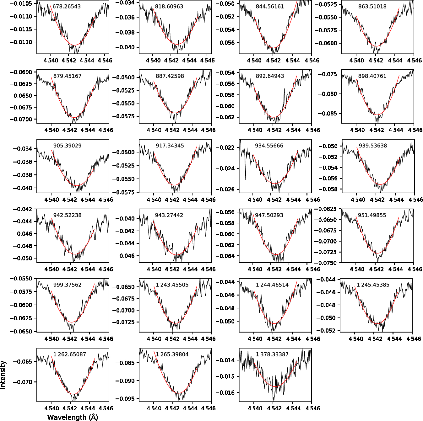
A total of 23 échelle spectra of Sp 3 were obtained with the High Resolution Spectrograph (HRS) on SALT (Bramall et al. Reference Bramall, Sharples and Tyas2010, Reference Bramall, Schmoll and Tyas2012; Crause et al. Reference Crause, Sharples and Bramall2014) under programmes 2016-2-SCI-034 and 2017-1-MLT-010 (PI: Miszalski). Table 1 gives a log of the observations taken with the medium resolution mode. We primarily use the blue arm data (resolving power  $R=\lambda/\Delta\lambda=43\,000$, for details see Miszalski et al. Reference Miszalski, Manick and Mikołajewska2018a). The basic data products (Crawford et al. Reference Crawford, Still and Schellart2010) were reduced with the midas pipeline developed by Kniazev, Gvaramadze & Berdnikov (Reference Kniazev, Gvaramadze and Berdnikov2016) which is based on the ECHELLE (Ballester Reference Ballester1992) and FEROS (Stahl, Kaufer & Tubbesing Reference Stahl, Kaufer and Tubbesing1999) packages. Heliocentric corrections were applied to the data using velset of the rvsao package (Kurtz & Mink Reference Kurtz and Mink1998). RV measurements in Table 1 were obtained by fitting single Voigt and two Gaussian functions to stellar He ii $\lambda4\,540$ and nebular H $\beta\ \lambda4\,861$ features, respectively, using the lmfit package (2016ascl.soft06014N). Figures 2 and 3 show the fits to the data. A weighted mean of the separation of the resolved H $\beta$ emission yields an expansion velocity of $2V_\mathrm{exp}=43.1\pm0.1\ \text{km s}^{-1}$ and a heliocentric RV of $43.5\pm0.1\ \text{km s}^{-1}$. The latter is in good agreement with $45.2\pm4.7\ \text{km s}^{-1}$ given by Durand, Acker & Zijlstra (Reference Durand, Acker and Zijlstra1998).
Log of SALT HRS observations of Sp 3. The Julian day represents the midpoint of each exposure and RV measurements are made from stellar He ii  $\lambda 4\,540$ and nebular H $\beta 4861$.

The observed stellar He ii  $\lambda 4\,541.59$ Å profiles (black lines) and the Voigt function fits (red lines). Each panel is labelled with the Julian day of each spectrum minus 2 457 000 d.
The observed nebular H $\beta \lambda4\,861.363$ Å profiles (black lines) and the multiple Gaussian function fits (red lines). Each panel is labelled with the Julian day of each spectrum minus 2 457 000 d.

2.3 Long-slit spectroscopy
Long-slit observations of Sp 3 were also conducted with RSS (Burgh et al. Reference Burgh, Nordsieck and Kobulnicky2003; Kobulnicky et al. Reference Kobulnicky, Nordsieck and Burgh2003) on 2018 June 11 under programme 2017-1-MLT-010 to measure the chemical abundances of the nebula. The 1.25 arcsec wide long slit was centred on the central star with a position angle (PA) of 104 deg to place the inner [O iii] lobes near the central star on the slit (see Figure 1(b) and Section 3.1). During the SALT track, exposures of 180 s and 1500 s were taken with the PG900 grating configured to cover 4 350–7 405 Å. This was then followed by a 1 500 s exposure taken with the PG2300 grating configured to cover 3 693–4 776 Å. The exposures were binned  $2\times2$ before read-out and the resulting approximate spectral resolutions measured from arc lamp emission lines were 4.80 and 1.75 Å, respectively. After basic reductions were performed by PYSALT (Crawford et al. Reference Crawford, Still and Schellart2010), cosmic ray events were cleaned using the lacosmic package (van Dokkum Reference van Dokkum2001) before the data were reduced using standard iraf routines such as identify, reidentify, fitcoords, and transform.
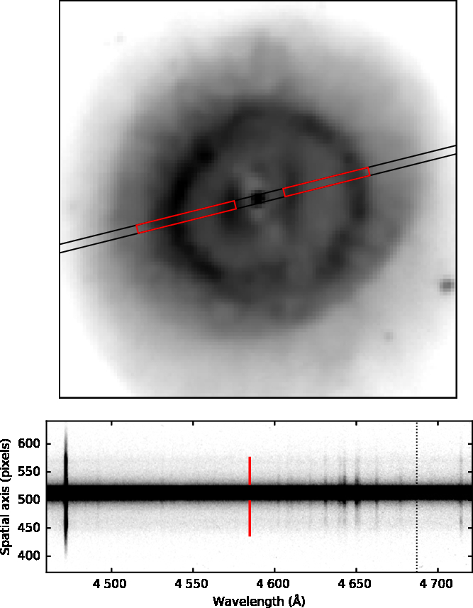
The PG2300 spectrum clearly showed optical recombination lines (ORLs) visible in the brightest inner part of the nebula (Figure 4). Figure 4 shows the two windows either side of the central star that were used to extract integrated spectra for chemical abundance analysis (Section 3.4) and the sky background was subtracted from regions well outside the whole nebula. The iraf task apall was used to extract spectra from these windows before being averaged into a single spectrum per observation. The same window was extracted from PG2300 and PG900 spectra relative to the trace of the central star determined by apall. Figure 5 shows the average spectra which were flux calibrated using spectra of the spectrophotometric standard stars EG274 (PG900) and G93-48 (PG2300). The absolute value of the flux calibration should only be considered to be approximate due to the moving pupil design of SALT. A separate spectrum of the central star was extracted and used to check that the relative calibration is smooth across both spectra, including in the overlap region, and that no additional features were imprinted onto the spectra due to flux calibration.
(Top panel) Position of the RSS 1.25 arcsec long slit with a PA of 104 deg (black rectangle) on the H $\alpha$ image of Sp 3 (Figure 1). Red rectangles of 15.2 arcsec (left) and 13.2 arcsec (right) indicate the apertures used to extract integrated spectra. Image dimensions are $60\times60$ $\text{arcsec}^2$ and the orientation is the same as Figure 1. (Bottom panel) Part of the PG2300 spectrum showing the nebular nature of the recombination lines near 4 650 Å. The dotted line indicates the expected location of the undetected He ii $\lambda 4\,686$ emission line. The same apertures as in the top panel are indicated by red lines either side of the central star. The spatial scale is 0.254 arcsec per pixel.
The average integrated RSS spectra extracted from the exposures taken with the PG2300 (top) and PG900 (bottom) gratings. Line identifications are listed in Table A1.
3. Analysis
3.1. Nebular morphology
Figure 1 reveals new morphological details not evident in previous images (Schwarz, Corradi & Melnick Reference Schwarz, Corradi and Melnick1992). Faint outer lobes appear to emerge in the H $\alpha$ image from a minor axis with a PA of $\sim 125$ deg. These lobes do not appear in the [O iii] image and are most prominent on the NW side of the nebula (Figure 1(d)). The outer lobes suggest the underlying morphology is bipolar. We measure a nebula radius of $\sim 34\,\text{arcsec}$ from a contour based on 10% of the average H $\alpha$ brightness in the inner nebula. The brightest features are an apparently broken ring of radius 14 arcsec and an inner pair of lobes that is brightest in [O iii]. These inner lobes are visible in Figure 1(b) near the central star and are brighter on the E and W sides of the central star. They are reminiscent of the inner [O iii] emission observed in the bipolar post-CE PN M2-19 (Miszalski et al. Reference Miszalski, Acker, Moffat, Parker and Udalski2009b). Several faint knots are located outside the main nebula with four to the NE and one to the SW (Figure 1(d)). Their appearance is similar to jets in the post-CE PN NGC 6337, which is viewed almost pole-on to the line of sight (e.g. NGC 6337, García-Díaz et al. Reference García-Díaz, Clark, López, Steffen and Richer2009). A thorough spatiokinematic study of the nebula is encouraged to further investigate its unusual morphology, jet system, and inclination angle. We discuss possible inclination angles further in Section 3.3.
3.2. Photospheric parameters and mass of the primary
Gauba et al. (Reference Gauba, Parthasarathy, Nakada and Fujii2001) examined low-resolution ( $R = \lambda/\Delta\lambda \approx 300$) ultraviolet (UV) spectra of the central star of Sp 3 obtained with the International Ultraviolet Explorer (IUE). They determined an O3V spectral type with an effective temperature of about $T_\mathrm{eff} = {50\,000}\,\mathrm{K}$ by comparison with the spectrophotometric standard star HD 93205. From the P-Cygni profile of the C iv $\lambda\lambda 1\,548, 1\,551$ Å resonance lines, they also measured a terminal wind velocity $v_\infty = 1603 \pm 400\ \text{km s}^{-1}$. From the presence of a stellar wind, they concluded that the surface gravity is log g < 5.2 cm s−2 (Cerruti-Sola & Perinotto Reference Cerruti-Sola and Perinotto1985). Guerrero & DeMarco (2013) found variability in the UV spectra, but not enough epochs were available to identify its cause.
To determine the stellar parameters of the primary, we corrected several individual orders of the blue HRS spectra for orbital motion (Table 1) and created average spectra around some strategic absorption lines that are suited for a detailed spectral analysis. Since non-local thermodynamic equilibrium (NLTE) atmosphere models are mandatory for such a hot star (e.g. Rauch et al. Reference Rauch, Demleitner, Hoyer and Werner2018), we employed the Tübingen non-LTE Model-Atmosphere Package (TMAPFootnote a; Werner et al. Reference Werner, Deetjen and Dreizler2003, Reference Werner, Dreizler and Rauch2012; Rauch & Deetjen Reference Rauch and Deetjen2003) to calculate plane-parallel models in radiative and hydrostatic equilibrium.
Since lines of H, He, C, and N are prominent in the observed spectra, we calculated two models composed of H + He and H + He + C + N with solar abundances adopted from Asplund et al. (Reference Asplund, Grevesse, Sauval and Scott2009) with  $T_\mathrm{eff} = {50\,000}\,\mathrm{K}$ and $\log g = {5.0}$ (Figure 6). For the H i and He ii lines, we find a good agreement between these models. The outer line wings of the H $\beta \text{/He}$ ii and H $\delta\text{/He}$ ii lines are too strong compared with the observed profiles, indicating a lower $\log g$.
Sections of the HRS spectra (black) compared with two synthetic spectra from models with  $T_\mathrm{eff} = {50\,000}\,\mathrm{K}$ and $\log g = {5.0}$ composed of He + He (blue, dashed line) and H + He + C + N (red, thick line). All abundances are solar. All spectra shown were convolved with Gaussians according to the HRS spectral resolution.
We calculated an extended grid of NLTE model atmospheres within 50 000 K ≲ T eff ≲ 82 000 K (with steps of 2 000 K), and 4.5 ≲ log g ≲ 5.0 (0.1) that consider opacities of H + He + C + N with solar abundances. While the outer lines wings of the H  $\beta \text{/He}$ ii and H $\delta \text{/He}$ ii blends are well reproduced at $\log g = {4.6 \pm 0.2}$, the theoretical line profiles of N v $\lambda\lambda\ 4\,604, 4\,620$ Å and C iv
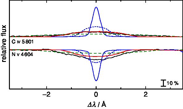
  $\lambda\lambda 5\,801, 5\,812 \Aring$ are much too narrow to reproduce the observed profiles. A significant rotation of v rot ≈ 80 km s−1 is necessary for a reasonable fit (Figure 7) and we adopt this value for our further analysis.
Comparison of the observed profiles of C iv  $\lambda 5\,801.31 \Aring$ and N v $\lambda 4\,603.74 \Aring$ (black lines) with profiles calculated from a model with $T_\mathrm{eff} = {68\,000}\,\mathrm{K}$ and $\log g = {4.6}$. The synthetic spectra are convolved with a rotational profile with $v_\mathrm{rot} = 0$ (blue, thin line), 40 (blue, dashed line), 80 (red line), and $120\,\text{km s}^{-1}$ (green, dashed line). The C and N mass fractions were adjusted to match the equivalent widths of the observed line profiles at $v_\mathrm{rot} = 80\,\text{km s}^{-1}$ in this figure.
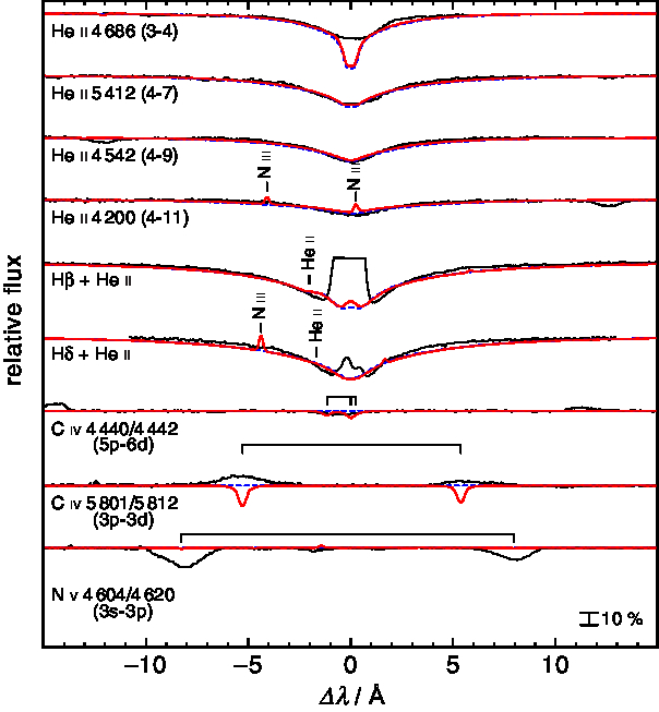
The determination of  $T_\mathrm{eff}$ is hampered because no lines of subsequent ionisation stages of one element could be identified in the available spectra to evaluate its ionisation equilibrium precisely. However, we found that in general, C iv $\lambda\lambda 5\,801, 5\,812~\Aring$ turns into emission only for $T_\mathrm{eff}$ $> 60\,000\,\mathrm{K}$, while C iv
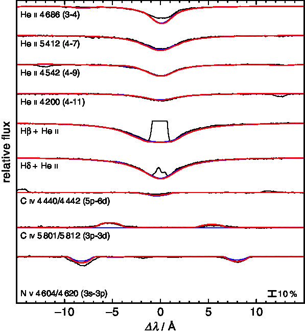
  $\lambda\lambda 4\,440, 4\,442 \Aring$ remains in absorption. Figure 8 shows a comparison of a model with $T_\mathrm{eff} = {68\,000}\,\mathrm{K}$ and $\log g = {4.6}$ to the observed spectra. All theoretical line profiles are in good agreement with the observations, but He ii $\lambda 4\,686.06 \Aring$ is much shallower than expected.
Same as in Figure 6, but for two models with  $T_\mathrm{eff} = {60\,000}\,\mathrm{K}$ (blue, thin line) and $T_\mathrm{eff} = {68\,000}\,\mathrm{K}$ (red, thick line), $\log g = {4.6}$, $\text{[H]} = 0.05, \text{[He]} = 0.02, \text{[C]} = -0.088, \text{and [N]} = 0.39$. [X] denotes log(fraction of element X / solar fraction of X). The synthetic spectra consider $v_\mathrm{rot} = 80\ \text{km s}^{-1}$.
The observed He ii  $\lambda 4\,686.06 \Aring$ line profile is obviously asymmetric, most likely due to problems in the data reduction. It is located at the red end of an HRS échelle order and the rectification of the outer red line wing is therefore difficult. The central depression, however, should not be affected significantly and this was confirmed independently by comparing the HRS spectrum with the PG900 RSS spectrum of the central star (Section 2). Rauch, Koeppen & Werner (Reference Rauch, Koeppen and Werner1996) have shown that due to a temperature inversion in the photosphere, an emission reversal in the line centre of He ii $\lambda 4\,686.06 \Aring$ is a sensitive indicator of $T_\mathrm{eff}$ because it strengthens with increasing $T_\mathrm{eff}$. The rapid stellar rotation is then responsible for a shallower line core at higher $T_\mathrm{eff}$. Figure 9 demonstrates this effect where we can reproduce the observed He ii $\lambda 4\,686.06 \Aring$ with a $T_\mathrm{eff} = {82\,000}\,\mathrm{K}$ and $\log g = {4.6}$ model. From N v $\lambda\lambda 4\,604, 4620 \Aring$, we have an additional constraint because it turns into emission for $T_\mathrm{eff}$ ***≳ 74 000 K (Figure 10). Furthermore, the H i/He ii blends become deeper than observed for $T_\mathrm{eff}$ ≳ 70 000 K. Thus, we adopt $T_\mathrm{eff} = {68\,000^{+12\,000}_{-6\,000}}\,\mathrm{K}$.
The HRS spectrum around He ii  $\lambda 4\,686.06 \Aring$ compared to three models with $\log g = {4.6}$ and different $T_\mathrm{eff}$ for $v_\mathrm{rot}=0 \text{km s}^{-1}$ (left) and $v_\mathrm{rot}=80 \text{km s}^{-1}$ (right).

Sections of the HRS spectrum (black) compared with synthetic spectra from models with  $T_\mathrm{eff}$ = 68 000, 72 000, 76 000, and 80 000 K, $\log g = {4.6}$, [H] = 0.05, [He] = 0.02, $\text{[C]} = -0.088$, and [N] = 0.39.

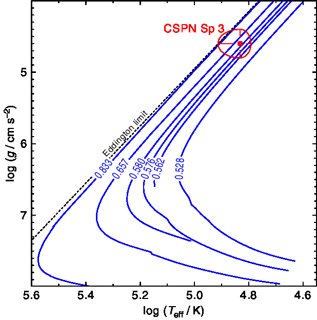
Figure 11 shows the CSPN of Sp 3 in the  $\log$ $T_\mathrm{eff}$ – $\log g$ diagram compared to stellar evolutionary tracks of H-rich post-AGB stars (Miller Bertolami Reference Miller Bertolami2016). We interpolate from these tracks a stellar mass of $M = 0.60^{+0.27}_{-0.05}\,{\rm M}_{\odot}$. From the tables of Miller Bertolami Reference Miller Bertolami2016, we determine a stellar luminosity of $\log (L\,/\,\,{\rm L}_{\odot}) = 3.85^{+0.55}_{-0.35}$. The position of Sp 3 in Figure 11 is consistent with a post-AGB origin, assuming these single star tracks are applicable to the binary central star, rather than the post-RGB origin suggested by Hillwig et al. (Reference Hillwig, Frew and Reindl2017). The location of the CSPN of Sp 3 is relatively close to the Eddington limit (Figure 11) and, thus, mass loss due to the stellar wind may have an impact on the spectral analysis, especially on the strengths of the C iv $\lambda\lambda 5\,801, 5\,812 \Aring$ emission lines. Table 2 summarises the results of our TMAP NLTE analysis.
Location of the CSPN of Sp 3 (with its error range) in the  $\log$ $T_\mathrm{eff}$ – $\log g$ plane. Post-AGB evolutionary tracks of H-rich stars [for about solar metallicity, $Z = 0.02$; (2016A A…588A.25M)] labelled with the stellar mass in $\,{\rm M}_{\odot}$, respectively, are shown for comparison. The dashed, black line indicates the Eddington limit for solar abundances.
Parameters of the CSPN of Sp 3 as derived by our TMAP NLTE analysis.

Notes: The abundance uncertainties are estimated to be  $\pm 0.5$ dex (including the error propagation from the $T_\mathrm{eff}$ and $\log g$ uncertainties).
To improve the spectral analysis, high-resolution UV spectroscopy with a high signal-to-noise ratio is highly desirable to investigate the wind properties and to determine  $T_\mathrm{eff}$ based on multiple ionisation equilibria of metal lines that form in the static region of the photosphere. Unfortunately, an available FUSE
Footnote b far-UV observation is strongly contaminated by interstellar line absorption and is thus not suitable for a precise spectral analysis. However, a P-Cygni profile of the O vi
$T_\mathrm{eff}$ based on multiple ionisation equilibria of metal lines that form in the static region of the photosphere. Unfortunately, an available FUSE
Footnote b far-UV observation is strongly contaminated by interstellar line absorption and is thus not suitable for a precise spectral analysis. However, a P-Cygni profile of the O vi  $\lambda\lambda 1\,032, 1\,038 \Aring$ resonance doublet is prominent in the FUSE observation (Id B032080100000, LWRS aperture, 9 439 s exposure time, TTAG mode, Figure 12), as expected from the presence of the C iv $\lambda\lambda 1\,548, 1\,551~\Aring$ P-Cygni profile in the IUE spectra (Gauba et al. Reference Gauba, Parthasarathy, Nakada and Fujii2001). A detailed re-analysis of the wind properties is beyond the scope of this paper.
Section of the FUSE observation around O vi  $\lambda\lambda$ 1032,1038 Å.

3.3 Orbital parameters
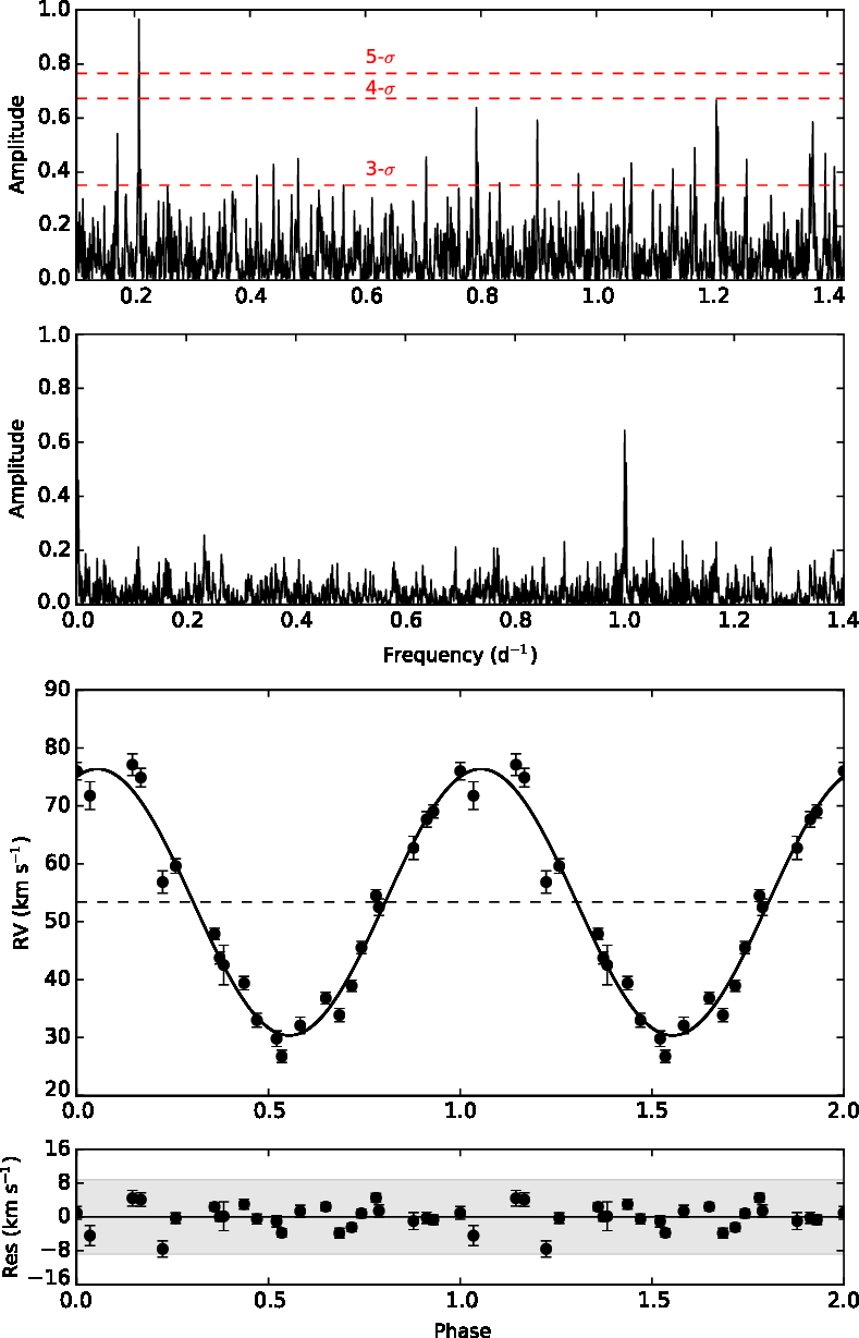
The SALT HRS RV measurements were analysed using a Lomb-Scargle periodogram (Press et al. Reference Press, Teukolsky, Vetterling and Flannery1992). The strongest peak in the periodogram displayed in Figure 13 is at  $f=0.208 \text{d}^{-1}$ and corresponds to an orbital period of 4.81 d. This orbital period was used as the basis for fitting a Keplerian orbit model that was built using a least-squares minimisation method applied to the phase-folded data. Figure 13 also shows the RV measurements phased with the orbital period, together with the Keplerian orbit fit and the residuals. Table 3 lists the orbital parameters determined from Monte Carlo simulations (for details, see Miszalski et al. Reference Miszalski, Manick and Mikołajewska2018a). An eccentric orbit is not supported by the Lucy & Sweeney (Reference Lucy and Sweeney1971) diagnostic test and we therefore fixed a circular orbit. Assuming the primary mass determined in Section 3.2, Figure 14 shows possible companion masses permitted by the mass function as a function of the orbital inclination.
Orbital parameters of the binary nucleus of Sp 3 derived from the best-fitting Keplerian orbit to He ii  $\lambda 4\,540$ measurements.
(Top panel) Lomb-scargle periodogram of the SALT HRS He ii  $\lambda 4\,540$ RV measurements (top half) and the window function (bottom half). The strongest peak at $f=0.208\ \text{d}^{-1}$ corresponds to the orbital period. (Bottom panel) SALT HRS RV measurements phased with the orbital period. The solid line represents the Keplerian orbit fit and the shaded region indicates the residuals are within $3\sigma$ of the fit, where $\sigma=2.94\ \text{km s}^{-1}$.
Companion masses permitted by the mass function in Table 3 for an assumed primary mass of  $M_1=0.60^{+0.27}_{-0.05}$ $\,{\rm M}_{\odot}$. The dotted lines indicate the corresponding uncertainty in the mass function.

A detailed spatiokinematic study of the nebula is required to constrain the orbital inclination of the binary which is expected to match the nebula orientation (Hillwig et al. Reference Henden, Templeton and Terrell2016). However, the apparent nebula morphology (Section 3.1) permits a first estimate of the orbital inclination. The bipolar lobes visible in Figure 1(d) could be produced by a bipolar nebula at an inclination of  $\sim 20$ deg to the line of sight (e.g. Model A in Figure 2 of Miszalski et al. Reference Miszalski, Acker, Moffat, Parker and Udalski2009b). The apparent broken ring feature (Section 3.1) may also be interpreted as the waist of a bipolar nebula viewed near pole-on (e.g. García-Díaz et al. Reference García-Díaz, Clark, López, Steffen and Richer2009). If the orbital inclination were $\sim 20$ deg, the companion mass in Figure 14 would suggest a companion mass of $\sim 0.6\,{\rm M}_{\odot}$, corresponding to a WD or a late K-type companion. At greater orbital inclinations, the companion mass would correspond to an M-dwarf companion; however, we note that this configuration with an 4.8-d orbital period would be considered anomalous in the context of the bias-corrected orbital period distribution of WD main-sequence binaries (Nebot Gómez-Morán et al. Reference Nebot, Gänsicke and Schreiber2011; see also Miszalski et al. Reference Miszalski, Acker, Moffat, Parker and Udalski2009b).
3.4. Nebular parameters and chemical abundances
We measured emission line fluxes from the RSS long-slit spectra using the automated line fitting algorithm program alfa (Wesson Reference Wesson2016). Each spectrum was analysed in two separate halves by alfa to better fit the emission line profiles. This was necessary to account for the slowly varying resolution with wavelength introduced by the volume-phase holographic gratings of RSS. Unsaturated measurements of the H $\alpha$ and [N ii]
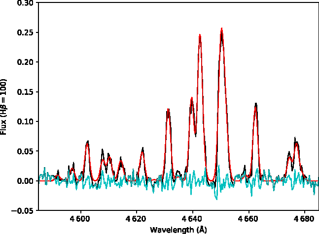
  $\lambda 6\,548, 6\,583 \Aring$ emission lines were taken from the 180-s PG900 spectrum. Figure 15 shows the alfa fits to the observed region around 4 650 Å which contains several nebular recombination lines due to O ii, N ii, and C iii.
The continuum-subtracted region of the PG2300 spectrum of Sp 3 near 4 650 Å, showing the observed spectrum (black), the alfa fit (red), and the residuals (cyan). The intensities have been normalised such that the integrated flux of H $\beta=100$.
We considered two possibilities to join the PG2300 and PG900 spectra into a single representative spectrum for chemical abundance analysis by the nebular empirical analysis tool neat (Wesson et al. Reference Werner, Dreizler and Rauch2012). First, we considered matching the measured fluxes of He i  $\lambda 4\,471 \Aring$ in the overlap region; however, this did not result in consistent measurements of the interstellar extinction from the H $\alpha\text{/H}\beta$ and H $\gamma\text{/H}\beta$ ratios. The He i temperatures based on the He i 5 876/4 471 and He i 6 678/4 471 ratios were also inconsistent with each other and with the O ii temperature. We therefore followed the approach taken by Wesson et al.(Reference Wesson, Jones, García-Rojas, Boffin and Corradi2018) where the scale factor was determined with neat such that the H $\alpha\text{/H}\beta$ and H $\gamma\text{/H}\beta$ ratios gave consistent measurements of the extinction. A modest scale factor of 0.9685 times the PG2300 spectrum was determined. All lines bluer than 4 800 Å in the final joined spectrum were then taken from the PG2300 spectrum scaled by this factor. The joined spectrum was analysed by neat and the identified emission lines are provided in Table A1. The average logarithmic extinction at $H\beta$, $c(H\beta)=0.06^{+0.05}_{-0.04}$, corresponding to $E(B-V)=0.09^{+0.07}_{-0.06}$ (Howarth 1983) is consistent with the previous estimate of $E(B-V)=0.16$ (Ciardullo et al. Reference Ciardullo, Bond and Sipior1999). Table 4 presents the electron density and temperature diagnostics, while Table 5 contains the ionic and total abundances plus calculated $\text{O}^{2+}$ and N adfs. The adfs are calculated as the ratio of the abundances determined from ORLs to those determined from collisionally excited lines (CELs).
Electron density and temperature diagnostics.
Ionic and total abundances for Sp 3.
4. DISCUSSION
4.1. Distance and likelihood of visual companion physical association
Could the visual companion identified by Ciardullo et al.(Reference Ciardullo, Bond and Sipior1999) be physically associated with the newly discovered post-CE central star, therefore making the nucleus a triple system? Ciardullo et al. 1999 argued that the small separation (0.31 arcsec) and characteristics of the companion are in agreement with the prior statistical distance estimates of the nebula, suggesting a true physical association. Stanghellini & Haywood Reference Stanghellini and Haywood2010 estimated a distance of  $1.92\pm 0.38$ kpc based on the nebula properties. Frew, Parker & Bojiˇci´c (2016) determined a G0V spectral type and a spectroscopic distance of $2.22^{+0.61}_{-0.48}$ kpc for the visual companion. Frew et al. (Reference Frew, Parker and Bojičić2016) also estimated a distance based on the nebular properties of $2.11\pm 0.60$ kpc, where the spectroscopic distance to the visual companion was used as a basis for including Sp 3 as a calibrator for their distance estimation method.
Despite the apparent agreement between all these distances, it is worthwhile to consider other independent distance measurements to check the suspected physical association of the visual companion, especially given the difficulties associated with estimating PN distances (Frew et al. Reference Frew, Parker and Bojičić2016). Here we consider distances estimated from the recent Gaia DR2 parallax measurement of the central star [Gaia Collaboration et al. (Reference Collaboration, Price-Whelan and Sipöcz2018a)] and the photospheric parameters of the primary we have derived from our TMAP NLTE analysis (Section 3.2).
Table 6 collates parameters recorded for the nucleus of Sp 3 in the second data release (DR2, Gaia Collaboration et al. Reference Collaboration, Price-Whelan and Sipöcz2018a) of the Gaia mission (Gaia Collaboration et al. Reference Collaboration, Prusti and de Bruijne2016) and other derived quantities.c The Gaia DR2 astrometry is affected by many systematic effects as discussed in papers associated with the data release (e.g. Lindegren et al. Reference Lindegren, Hernandez and Bombrun2018; Gaia Collaboration et al. Reference Collaboration, Price-Whelan and Sipöcz2018b; Arenou et al. Reference Arenou, Luri and Babusiaux2018). Distance determination is not necessarily a straightforward exercise of taking the reciprocal of the parallax (Luri et al. Reference Luri, Brown and Sarro2018) and a Bayesian approach is the preferred method (Bailer-Jones et al. Reference Bailer-Jones, Rybizki, Fouesneau, Mantelet and Andrae2018). Furthermore, in the case of PNe the nebula may introduce additional biases (Kimeswenger & Barría Reference Kimeswenger and Barría2018), though the full extent of such biases is yet to be determined. The catalogue of Bailer-Jones et al. (Reference Bailer-Jones, Rybizki, Fouesneau, Mantelet and Andrae2018) provides robust distance estimates for Gaia DR2 sources. Distance estimates in the catalogue include lower and upper boundaries of the highest density interval around the mode of the posterior with probability  $p=0.6827$. A Gaussian posterior would correspond to an uncertainty of $\pm1\sigma$ in the distance.
Gaia DR2 parameters and derived quantities for the central star of Sp 3. The parallax  $\varpi$ includes a zero-point correction of $+0.029$ mas (see Lindegren et al. Reference Lindegren, Hernandez and Bombrun2018). Filters adopted by Gaia Collaboration et al.(Reference Collaboration, Price-Whelan and Sipöcz2018b), indicated by inequalities and thresholds (enclosed in parentheses) for the relevant values, are all satisfied in the cases shown here.
In the case of Sp 3, the Bailer-Jones et al. (Reference Bailer-Jones, Rybizki, Fouesneau, Mantelet and Andrae2018) estimate of  $r_\mathrm{est}=11.2 \text{kpc}$, with boundaries of $r_\mathrm{lo}=8.1 \text{kpc}$ and $r_\mathrm{hi}=15.4\ \text{kpc}$, unfortunately appears to be too distant. At 11.2 kpc, the 34 arcsec nebula radius (Section 3.1) would correspond to $\sim 1.85$ pc, considerably larger than most PNe (Frew et al. Reference Frew, Parker and Bojičić2016). The morphology of such a large nebula would more closely resemble evolved, low-surface-brightness PNe, e.g. PFP1 (Pierce et al. Reference Pierce, Frew, Parker and Köppen2004), inconsistent with the observed appearance of Sp 3 (Section 3.1). Given the implausible nature of this result, we have no other recourse but to estimate the distance as the reciprocal of the parallax to obtain $d=2.32^{+0.79}_{-0.47}\ \text{kpc}$. Despite the difficulties associated with this approach (Luri et al. Reference Luri, Brown and Sarro2018), we are somewhat reassured by the fact that the parameters in Table 6 satisfy several quality criteria filters, namely in the form of inequalities and thresholds, that are applied to Gaia DR2 data of large samples before analysis (Section 2.1 of Gaia Collaboration et al. Reference Collaboration, Price-Whelan and Sipöcz2018b; see also Lindegren et al. Reference Lindegren, Hernandez and Bombrun2018 and Arenou et al. Reference Arenou, Luri and Babusiaux2018).
We have also calculated the spectroscopic distance of the CSPN of Sp 3 using the flux calibration of Heber et al. (Reference Heber, Hunger, Jonas and Kudritzki1984) for  $\lambda_\mathrm{eff} = 5454 \Aring$,
 $$d[\mathrm{pc}]=7.11 \times 10^{-4} \cdot \sqrt{H_\nu\cdot M \times 10^{0.4\, m_{\mathrm{v}_0}-\log g}} ,$$
with  $m_\mathrm{V_o} = m_\mathrm{V} - 2.175 c$, $c = 1.47 E_\mathrm{B-V}$, and the Eddington flux $H_\nu$ ( $1.52\times 10^{-3} \text{erg/cm}^{2}\text{/s/Hz}$) at 5454 Å of our final model atmosphere. We use $m_{\mathrm{V}}=12.89$ that was measured by Zacharias et al. (Reference Zacharias, Finch and Girard2013) and Henden et al. (Reference Henden, Templeton and Terrell2016). With $E_\mathrm{B-V}=0.14 \pm 0.05$ (Figure 16) and $M = 0.60^{+0.27}_{-0.05}$, we derived $d=2.8^{+0.8}_{-0.7}\,\text{kpc}$. Regarding the He ii $\lambda 4\,686.06 \Aring$ discrepancy (see Section 3.2), we find better agreement between model and observation at about $T_\mathrm{eff} = {80\,000}\,\mathrm{K}$. However, then the star is already located very close to the Eddington limit (Figure 11) and, thus, would be more massive $M = 0.83^{+0.18}_{-0.08}$ and at a much further distance of $d=4.0^{+0.9}_{-1.2}\,\text{kpc}$. This distance is around two times further than the other distance estimates and seems unlikely.
Determination of for the CSPN of Sp 3 using the FUSE spectrum (Id B032080100000 retrieved from the MAST archive; black line) and the B and V (Zacharias et al. Reference Zacharias, Finch and Girard2013; Hendenet al. 2016) and the 2MASS J, H, and  $K_s$ magnitudes (Cutri et al. Reference Cutri, Skrutskie and van Dyk2003). The model has $T_\mathrm{eff} = {68\,000}\,\mathrm{K}$ and $\log g = {4.6}$ and is normalised to the $K_s$ magnitude (red line). The blue lines indicate the error range.
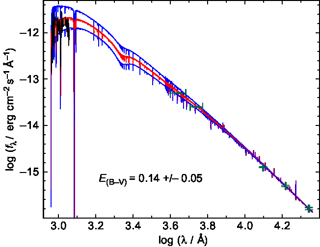
Table 7 provides a summary of the various distance estimates to Sp 3. While the actual veracity of the distance obtained from the reciprocal of the parallax may only become clear once additional observations and improved data processing are available from future Gaia data releases, the overall picture is one that clearly supports a likely physical association between the visual companion and the post-CE binary nucleus of Sp 3.
A summary of various distances to Sp 3.
4.2. Chemical abundances
The most prominent result is that the adf( $\text{O}^{2+}$) of $24.6^{+4.1}_{-3.4}$ lies in the ‘extreme’ range ( $\text{adf} > 10$) for PNe (Wesson et al. Reference Wesson, Jones, García-Rojas, Boffin and Corradi2018). Wesson et al.(Reference Wesson, Jones, García-Rojas, Boffin and Corradi2018) identified several trends with adf( $\text{O}^{2+}$) that post-CE PNe follow concerning the [S ii] and [O ii] electron densities, as well as the O/H and N/H abundances. The location of Sp 3 with its low nebular densities and ‘extreme’ adf is evidently consistent with these trends, though their cause is not yet clear (Wesson et al. Reference Wesson, Jones, García-Rojas, Boffin and Corradi2018).
Wesson et al. (Reference Wesson, Jones, García-Rojas, Boffin and Corradi2018) also found that only post-CE PNe with orbital periods less than  $\sim 1.15$ d demonstrated ‘extreme’ adfs. Figure 17 depicts the adf( $\text{O}^{2+}$) as a function of orbital period constructed using data from Table 6 of Wesson et al. (Reference Wesson, Jones, García-Rojas, Boffin and Corradi2018). We have added Sp 3, together with MyCn 18 ( $P=18.15$ d, Miszalski et al. Reference Miszalski, Manick and Mikołajewska2018b; adf $(\mathrm{O}^{2+})=1.8$, Tsamis et al. Reference Tsamis, Barlow, Liu, Storey and Danziger2004) and NGC 2392 ( $P=1.9$ d, Miszalski et al. Reference Miszalski, Acker, Moffat, Parker and Udalski2009a; adf $(\mathrm{O}^{2+})=1.65$, Zhang et al. Reference Zhang, Fang and Chau2012). The orbital period of IC 4776 was revised down to 3.11 d (Miszalski et al. Reference Miszalski, Acker, Moffat, Parker and Udalski2009b) and we excluded Hen 2-161 whose orbital period is uncertain. The 4.8-d orbital period of Sp 3 clearly breaches the expected tendency for multiple day orbital period post-CE to show normal adfs (Wesson et al. Reference Wesson, Jones, García-Rojas, Boffin and Corradi2018), making it a clear outlier in Figure 17.
The location of Sp 3 amongst other post-CE PNe with measured adfs and orbital periods. Post-CE PNe with orbital periods in excess of 1.0 d are labelled. The dotted lines mark the thresholds of Wesson et al.(Reference Wesson, Jones, García-Rojas, Boffin and Corradi2018) indicative of ‘normal’ ( $\text{adf} < 5$), ‘elevated’ ( $5< \text{adf} <10$), and ‘extreme’ ( $\text{adf} >10$) adfs. Sp 3 occupies a previously unpopulated part of the parameter space.
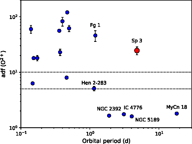
The extreme adf of Sp 3 emphasises the presence of strong selection effects in the known post-CE PN orbital period distribution. We consider any relationships inferred between the adf and orbital period to therefore not be meaningful, especially given the still very small population of post-CE PNe with determined adfs. These selection effects are primarily determined by the use of photometric monitoring to discover most post-CE PNe (e.g. Miszalski et al. Reference Miszalski, Acker, Moffat, Parker and Udalski2009a).Indeed, we note that all post-CE PNe with orbital periods above 1.0 d in Figure 17 were identified via RV monitoring except Hen 2-283!
The He abundance ( $12+\log(\mathrm{He/H})=11.11$ dex) and $\log(\mathrm{N/O})=0.05$ dex are typical of Type I PNe (Kingsburgh & Barlow Reference Kingsburgh and Barlow1994) that are believed to form from more massive progenitors ( $M\sim3 \,{\rm M}_{\odot}$, Karakas & Lattanzio Reference Karakas and Lattanzio2014), making Sp 3 one of very few Type I PNe amongst post-CE PNe (Corradi et al.
2014). The apparent bipolar morphology (Section 3.1) is also consistent with the Type I abundance pattern (Corradi & Schwarz Reference Corradi and Schwarz1995). The oxygen abundance ( $0.46$ dex below Solar, Asplund et al. Reference Asplund, Grevesse, Sauval and Scott2009) and the height below the Galactic plane ( $z=-0.57 \text{kpc}$ assuming $d=2.32 \text{kpc}$, Section 4.1) both suggest Sp 3 belongs to the thick disk of the Galaxy (e.g. Robin et al. Reference Robin, Reylé and Fliri2014).
5. Conclusions
We have presented a SALT study of the PN Sp 3 and its central star for which Ciardullo et al. (Reference Ciardullo, Bond and Sipior1999) previously identified to have a visual companion located 0.31 arcsec away. RV measurements obtained with SALT HRS reveal the central star to be a post-CE binary with an orbital period of 4.81 d. The spectroscopic distance of the visual companion ( $2.22^{+0.61}_{-0.48} \text{kpc}$, Frew et al. Reference Frew, Parker and Bojičić2016) is in agreement with estimates of the distance to Sp 3 based on the nebula properties ( $1.92\pm0.38 \text{kpc}$, Stanghellini & Haywood Reference Stanghellini and Haywood2010; $2.11\pm0.60 \text{kpc}$, Frew et al. Reference Frew, Parker and Bojičić2016), the GAIA DR2 parallax of the central star ( $2.32^{+0.79}_{-0.47} \text{kpc}$, Gaia Collaboration et al. Reference Collaboration, Price-Whelan and Sipöcz2018a), and the photospheric properties of the central star ( $2.8^{+0.8}_{-0.7} \text{kpc}$). This strongly suggests that the visual companion is associated with the post-CE binary nucleus, indicating that nucleus of Sp 3 is a likely triple system. This is the strongest candidate for a triple nucleus of a PN besides the only proven case of NGC 246 (Adam & Mugrauer Reference Adam and Mugrauer2014).
Our main conclusions are as follows:
A total of 23 SALT HRS RV measurements find the nucleus of Sp 3 to be a spectroscopic binary with an orbital period of 4.81 d and an RV semi-amplitude of $22.92\pm0.51 \text{km s}^{-1}$. This is one of the longest orbital periods known in PNe (Miszalski et al. Reference Miszalski, Manick, VanWinckel and Escorza2019b) and higher than expected for post-CE WD main-sequence binaries (Nebot Gómez-Morán et al. Reference Nebot, Gänsicke and Schreiber2011), further supporting the possibility that there may be a larger population of longer orbital period binary central stars waiting to be found. Sp 3 is the third binary we have identified in the list of RV variables identified by Afšar & Bound Af(Miszalski et al. Reference Miszalski, Manick and Mikołajewska2018a) and NGC 2392 (Miszalski et al. Reference Miszalski, Manick, VanWinckel and Escorza2019a).
The TMAP NLTE model atmosphere analysis of the SALT HRS spectra shows the primary to be a relatively fast rotator (
$v_\mathrm{rot}=80\pm20 \text{km s}^{-1}$) with $T_\mathrm{eff}=68\,000^{+12\,000}_{-6\,000}$ K and $\log g=4.6\pm0.2$. Interpolation with the H-rich stellar evolutionary tracks of Miller Bertolami (Reference Miller Bertolami2016) shows that the central star is relatively close to the Eddington limit with $M=0.60^{+0.27}_{-0.05}$ $\,{\rm M}_{\odot}$ and log ($L/\,{\rm L}_{\odot}$)=$3.85^{+0.55}_{-0.35}$. High-resolution UV spectroscopy is required to further investigate the wind properties identified by previous studies [Gauba et al. Reference Gauba, Parthasarathy, Nakada and Fujii2001; Guerrero & De Marco (2013)] and refine the photospheric parameters.SALT RSS Fabry-Pérot H
$\alpha$ and [O iii] images are presented of the peculiar nebula, revealing new structures that include faint bipolar lobes, jets and a broken ring that may be the waist of a bipolar nebula. The orientation of the nebula is estimated to be $\sim 20$ deg; however, detailed spatiokinematic study is required to properly constrain the orientation. Assuming the orientation matches the orbital inclination (Hillwig et al. Reference Henden, Templeton and Terrell2016) and adopting $M_1=0.60^{+0.27}_{-0.05}$ $\,{\rm M}_{\odot}$, the mass function of the binary central star gives a companion mass of $\sim0.6 \,{\rm M}_{\odot}$, corresponding to a WD or possibly K-dwarf companion.SALT RSS long-slit spectroscopy of the nebula was used to determine the nebular chemical abundances. Most surprising is the extreme adf(
$\text{O}^{2+}$) of $24.6^{+4.1}_{-3.4}$, which does not fit the expected low adf of post-CE PNe with orbital periods longer than $\sim 1$ d (Wesson et al. Reference Wesson, Jones, García-Rojas, Boffin and Corradi2018). Selection effects are therefore playing a dominant role in the current search for trends amongst post-CE PNe.The chemical abundance pattern of the nebula is typical of Type I PNe (
$12+\log(\mathrm{He/H})=11.11\ \text{dex}; \log(\mathrm{N/O})=0.05 \text{dex}$), thought to evolve from more massive progenitors (Corradi & Schwarz 1995; Karakas & Lattanzio Reference Karakas and Lattanzio2014). However, the sub-solar oxygen abundance and large height below the Galactic plane suggest a thick disc membership for Sp 3. This paradox may be attributable to the still poorly understood influence of rotation ($v_\mathrm{rot}=80\,\pm\,20\ \text{km s}^{-1}$) and binarity on AGB nucleosynthesis (e.g. Stasi´nska et al. 2010; Miszalski et al. Reference Miszalski, Boffin and Frew2012; Karakas & Lattanzio Reference Karakas and Lattanzio2014 and ref. therein), though we note that Type I PNe remain under-represented amongst post-CE PNe (Corradi et al. Reference Corradi, Rodríguez-Gil and Jones2014).It is unclear whether the triple nature of the nucleus has influenced the nebula morphology given its large separation from the binary component (
$\sim 740 \text{au}$, Ciardullo et al. Reference Ciardullo, Bond and Sipior1999). The current orbit of the post-CE nucleus is circular; however, it is interesting to conjecture that the tertiary component may have induced an eccentric orbit in the past via the Kozai–Lidov mechanism (e.g. Toonen et al. Reference Toonen, Hamers and Portegies Zwart2016).Further modelling of the potential influence of the triple system on the nebula would be of interest.


Acknowledgements
BM acknowledges support from the National Research Foundation (NRF) of South Africa and thanks the Institute of Astronomy at KU Leuven for their hospitality. RM acknowledges support from the Claude Leon Foundation. We thank an anonymous referee for constructive comments that helped improve this paper. This paper is based on observations made with the SALT under programmes 2012-1-RSA_OTH-010, 2016-2-SCI-034 and 2017-1-MLT-010 (PI: B. Miszalski). We are grateful to our SALT colleagues for maintaining the telescope facilities and conducting the observations. We thank S. Mohamed and D. Kamath for discussions, R. Wesson for assistance with his alfa and neat software, A.Y. Kniazev for making available his HRS pipeline data products, and T.E. Pickering for RSS Fabry-Pérot technical assistance. Polish participation in SALT is funded by grant no. MNiSW DIR/WK/2016/07. This research has been partly founded by the National Science Centre, Poland, through grant OPUS 2017/27/B/ST9/01940 to JM. KI has been financed by the Polish Ministry of Science and Higher Education Diamond Grant Programme via grant 0136/DIA/2014/43 and by the Foundation for Polish Science (FNP) within the START program. HVW and RM acknowledge support from the Belgian Science Policy Office under contract BR/143/A2/STARLAB. HVW acknowledges additional support from the Research Council of KU Leuven under contract C14/17/082. Some of the data presented in this paper were obtained from the Barbara A. Mikulski Archive for Space Telescopes (MAST). STScI is operated by the Association of Universities for Research in Astronomy, Inc., under NASA contract NAS5-26555. Support for MAST for non-HST data is provided by the NASA Office of Space Science via grant NNX09AF08G and by other grants and contracts. This research has made use of NASA’s Astrophysics Data System and the SIMBAD database, operated at CDS, Strasbourg, France. This research made use of Matplotlib (Hunter Reference Hunter2007) and Astropy,Footnote d a community-developed core Python package for Astronomy Collaboration et al. (Reference Collaboration, Robitaille and Tollerud2013; Reference Collaboration, Price-Whelan and Sipöcz2018). IRAF is distributed by the National Optical Astronomy Observatory, which is operated by the Association of Universities for Research in Astronomy (AURA) under a cooperative agreement with the National Science Foundation. This work has made use of data from the European Space Agency (ESA) mission Gaia (https://www.cosmos.esa.int/gaia), processed by the Gaia Data Processing and Analysis Consortium (DPAC, https://www.cosmos.esa.int/web/gaia/dpac/consortium). Funding for the DPAC has been provided by national institutions, in particular the institutions participating in the Gaia Multilateral Agreement.
Observed  $F(\lambda)$ and dereddened $I(\lambda)$ emission line fluxes for Sp 3.