 ¬
¬ ¬
¬








1 Introduction
Over more than two decades, research in logic programming has shifted toward studying and efficiently implementing fragments that are sufficiently expressive for demanding practical applications. Answer Set Programming (ASP) exemplifies this trend: despite not being Turing-complete, ASP has found diverse applications and gained broad acceptance as a robust paradigm. Recent investigations have explored extending ASP “beyond $\mathsf{NP}$
” (Bogaerts et al. Reference Bogaerts, Janhunen and Tasharrofi2016; Amendola et al. Reference Amendola, Ricca and Truszczynski2019; Fandinno et al. Reference Fandinno, Laferrière, Romero, Schaub and Son2021). More recently, Higher-Order Datalog with negation (Bogaerts et al. Reference Bogaerts, Charalambidis, Chatziagapis, Kostopoulos, Pollaci and Rondogiannis2024) has been proposed as a powerful candidate for such an extension. In particular, it has been shown (Charalambidis et al. Reference Charalambidis, Kostopoulos, Nomikos and Rondogiannis2025) that
$\mathsf{NP}$
” (Bogaerts et al. Reference Bogaerts, Janhunen and Tasharrofi2016; Amendola et al. Reference Amendola, Ricca and Truszczynski2019; Fandinno et al. Reference Fandinno, Laferrière, Romero, Schaub and Son2021). More recently, Higher-Order Datalog with negation (Bogaerts et al. Reference Bogaerts, Charalambidis, Chatziagapis, Kostopoulos, Pollaci and Rondogiannis2024) has been proposed as a powerful candidate for such an extension. In particular, it has been shown (Charalambidis et al. Reference Charalambidis, Kostopoulos, Nomikos and Rondogiannis2025) that $k+1$
-order Datalog with negation,
$k+1$
-order Datalog with negation, $k\geq 1$
, captures
$k\geq 1$
, captures $k-\textsf {EXPTIME}$
under the well-founded semantics, and captures co-
$k-\textsf {EXPTIME}$
under the well-founded semantics, and captures co- $k$
-
$k$
- $\mathsf{NEXPTIME}$
and
$\mathsf{NEXPTIME}$
and $k$
-
$k$
- $\mathsf{NEXPTIME}$
under the stable model semantics for cautious and brave reasoning, respectively. However, this power comes at a cost: increased expressiveness inevitably places a significant burden on implementation. Consequently, identifying a fragment of Higher-Order Datalog with negation that can express problems beyond
$\mathsf{NEXPTIME}$
under the stable model semantics for cautious and brave reasoning, respectively. However, this power comes at a cost: increased expressiveness inevitably places a significant burden on implementation. Consequently, identifying a fragment of Higher-Order Datalog with negation that can express problems beyond $\mathsf{NP}$
and that is still amenable to efficient implementation, remains a major challenge.
$\mathsf{NP}$
and that is still amenable to efficient implementation, remains a major challenge.
A promising avenue of research is the study of a linear fragment of Higher-Order Datalog with negation. In the first-order Datalog setting, linearity is a pivotal property defined by restricting every rule body to contain at most one recursive atom (Ullman Reference Ullman1989, Chapter 15). This restriction is practically significant for two reasons. First, it is widely recognized that Linear Datalog suffices to express most “real-life” recursive queries, see, for example (Consens and Mendelzon Reference Consens and Mendelzon1990, p. 405). Second, from an implementation standpoint, Linear Datalog is far more amenable to specialized optimizations than full Datalog (Ullman Reference Ullman1989). Theoretically, this efficiency is formalized by the fact that Linear Datalog captures $\mathsf{NL}$
(Nondeterministic Logarithmic Space) on ordered databases (Dantsin et al. Reference Dantsin, Eiter, Gottlob and Voronkov2001). Intuitively, this implies that a query can be evaluated using logarithmic space relative to the input size. In practical terms, the evaluation engine need not store the entire history of derivations, but only the current state of the computation (e.g., the “current node” in a traversal). This favorable complexity profile extends to programs with negation: it has been shown that Stratified Linear Datalog - where rules are limited to linear recursion within the same stratum - also captures
$\mathsf{NL}$
(Nondeterministic Logarithmic Space) on ordered databases (Dantsin et al. Reference Dantsin, Eiter, Gottlob and Voronkov2001). Intuitively, this implies that a query can be evaluated using logarithmic space relative to the input size. In practical terms, the evaluation engine need not store the entire history of derivations, but only the current state of the computation (e.g., the “current node” in a traversal). This favorable complexity profile extends to programs with negation: it has been shown that Stratified Linear Datalog - where rules are limited to linear recursion within the same stratum - also captures $\mathsf{NL}$
on ordered databases (Consens and Mendelzon Reference Consens and Mendelzon1990). It is therefore interesting (and potentially practical) to investigate what linearity means in a higher-order setting and its precise expressive power.
$\mathsf{NL}$
on ordered databases (Consens and Mendelzon Reference Consens and Mendelzon1990). It is therefore interesting (and potentially practical) to investigate what linearity means in a higher-order setting and its precise expressive power.
In this paper, we undertake the study of the above question. We generalize the concept of Stratified Linear Datalog to the higher-order setting, getting a language which in the rest of the paper we will refer to as Stratified Linear Higher-Order Datalog $^\neg$
. Our extension is based on the notion of stratification introduced by Bogaerts et al. (Reference Bogaerts, Charalambidis, Chatziagapis, Kostopoulos, Pollaci and Rondogiannis2024), which ensures programs are stratified not only with respect to negation but also with respect to higher-order application. Our central contribution proves that for all
$^\neg$
. Our extension is based on the notion of stratification introduced by Bogaerts et al. (Reference Bogaerts, Charalambidis, Chatziagapis, Kostopoulos, Pollaci and Rondogiannis2024), which ensures programs are stratified not only with respect to negation but also with respect to higher-order application. Our central contribution proves that for all $k \ge 1$
, the
$k \ge 1$
, the $(k+1)$
-order fragment of Stratified Linear Higher-Order Datalog
$(k+1)$
-order fragment of Stratified Linear Higher-Order Datalog $^\neg$
captures
$^\neg$
captures $(k-1)-\textsf {EXPSPACE}$
. Unlike the first-order setting where an ordered database is required to capture
$(k-1)-\textsf {EXPSPACE}$
. Unlike the first-order setting where an ordered database is required to capture $\mathsf{NL}$
, our higher-order characterization holds without any such ordering assumption. Since
$\mathsf{NL}$
, our higher-order characterization holds without any such ordering assumption. Since $k-\textsf {EXPSPACE}$
is a subset of the
$k-\textsf {EXPSPACE}$
is a subset of the $k-\textsf {EXPTIME}$
class captured by the unrestricted Higher-Order Datalog
$k-\textsf {EXPTIME}$
class captured by the unrestricted Higher-Order Datalog $^\neg$
language (Charalambidis et al. Reference Charalambidis, Kostopoulos, Nomikos and Rondogiannis2025), our results indicate that, potentially, linearity leads to a more “manageable” language from an implementation point of view. Table 1 shows more compactly the aforementioned results: the second row is new, the first one is from (Charalambidis et al. Reference Charalambidis, Kostopoulos, Nomikos and Rondogiannis2025). Surprisingly, our results have a direct correspondence with Neil Jones’ results (Jones Reference Jones2001) on the expressive power of the tail-recursive fragments of a restricted higher-order functional language. Given the close conceptual link between tail-recursion and linearity, it is remarkable but not totally unexpected that these distinct programming paradigms capture identical complexity hierarchies.
$^\neg$
language (Charalambidis et al. Reference Charalambidis, Kostopoulos, Nomikos and Rondogiannis2025), our results indicate that, potentially, linearity leads to a more “manageable” language from an implementation point of view. Table 1 shows more compactly the aforementioned results: the second row is new, the first one is from (Charalambidis et al. Reference Charalambidis, Kostopoulos, Nomikos and Rondogiannis2025). Surprisingly, our results have a direct correspondence with Neil Jones’ results (Jones Reference Jones2001) on the expressive power of the tail-recursive fragments of a restricted higher-order functional language. Given the close conceptual link between tail-recursion and linearity, it is remarkable but not totally unexpected that these distinct programming paradigms capture identical complexity hierarchies.
Expressive power results (entries with a “ $*$
” use the ordering assumption)
$*$
” use the ordering assumption)

In conclusion, the main contributions of the present paper can be summarized as follows:
-
• Extension of linearity: We extend the classical notion of linearity to the class of higher-order Datalog programs. We believe that this extension establishes the basis for developing novel optimizations for higher-order logic programming.
-
• Lower bound simulation: We provide a simulation of space-bounded Turing machines using Stratified Linear Higher-Order Datalog $^\neg$
, using higher-order predicates to encode the counting of the tape-space of the Turing machine, its configurations, and its execution. The simulation is natural and does not require any tedious encodings. This simplicity suggests that the proposed language is not merely a theoretical construct, but a natural and intuitive fragment of Higher-Order Datalog
$^\neg$
.
$^\neg$
, using higher-order predicates to encode the counting of the tape-space of the Turing machine, its configurations, and its execution. The simulation is natural and does not require any tedious encodings. This simplicity suggests that the proposed language is not merely a theoretical construct, but a natural and intuitive fragment of Higher-Order Datalog
$^\neg$
. -
• Upper bound and space efficient evaluation: We present a space-efficient proof procedure for computing queries. By using top-down evaluation, we avoid the full program interpretation, which would otherwise consume space that is tower-exponential in the order of the program. We believe that a refinement of our proof procedure could lead to a viable implementation of the proposed language.


Sections 2 and 3 introduce the syntax, semantics, and motivation for Stratified Linear Higher-Order Datalog $^\neg$
. Sections 4, 5, and the supplementary material establish theoretical space complexity bounds and the correctness proof of the space-efficient evaluation algorithm.
$^\neg$
. Sections 4, 5, and the supplementary material establish theoretical space complexity bounds and the correctness proof of the space-efficient evaluation algorithm.
2 Higher-Order Datalog with negation: Preliminaries
In this section we introduce the syntax of Higher-Order Datalog $^\neg$
, following Bogaerts et al. (Reference Bogaerts, Charalambidis, Chatziagapis, Kostopoulos, Pollaci and Rondogiannis2024). The language uses two base types:
$^\neg$
, following Bogaerts et al. (Reference Bogaerts, Charalambidis, Chatziagapis, Kostopoulos, Pollaci and Rondogiannis2024). The language uses two base types: $o$
, the Boolean domain, and
$o$
, the Boolean domain, and $\iota$
, the domain of data objects. The composite types are partitioned into predicate ones (assigned to predicate symbols) and argument ones (assigned to parameters of predicates).
$\iota$
, the domain of data objects. The composite types are partitioned into predicate ones (assigned to predicate symbols) and argument ones (assigned to parameters of predicates).
Definition 2.1. Types are either predicate or argument, denoted by $\pi$
and
$\pi$
and $\rho$
respectively, and defined as:
$\rho$
respectively, and defined as:
 \begin{align*} \pi & := o \mid (\rho \to \pi ) \\ \rho & := \iota \mid \pi \end{align*}
The binary operator $\to$
is right-associative. Every predicate type
$\to$
is right-associative. Every predicate type $\pi$
can be written in the form
$\pi$
can be written in the form $\rho _1 \to \cdots \to \rho _n \rightarrow o$
,
$\rho _1 \to \cdots \to \rho _n \rightarrow o$
, $n\geq 0$
(for
$n\geq 0$
(for $n=0$
we assume that
$n=0$
we assume that $\pi =o$
).
$\pi =o$
).
Definition 2.2. The alphabet of Higher-Order Datalog $^\neg$
consists of: predicate variables of every predicate type
$^\neg$
consists of: predicate variables of every predicate type $\pi$
(denoted by capital letters such as
$\pi$
(denoted by capital letters such as $\mathsf{P},\mathsf{Q},\ldots )$
; predicate constants of every predicate type
$\mathsf{P},\mathsf{Q},\ldots )$
; predicate constants of every predicate type $\pi$
(denoted by lowercase letters such as
$\pi$
(denoted by lowercase letters such as $\mathsf{p},\mathsf{q},\ldots$
); individual variables of type
$\mathsf{p},\mathsf{q},\ldots$
); individual variables of type $\iota$
(denoted by capital letters such as
$\iota$
(denoted by capital letters such as $\mathsf{X},\mathsf{Y},\ldots$
); individual constants of type
$\mathsf{X},\mathsf{Y},\ldots$
); individual constants of type $\iota$
(denoted by lowercase letters such as
$\iota$
(denoted by lowercase letters such as $\mathsf{a},\mathsf{b},\ldots$
); the equality constant
$\mathsf{a},\mathsf{b},\ldots$
); the equality constant $\approx$
of type
$\approx$
of type $\iota \to \iota \to o$
; the conjunction constant
$\iota \to \iota \to o$
; the conjunction constant $\wedge$
of type
$\wedge$
of type $o \to o \to o$
; the inverse implication constant
$o \to o \to o$
; the inverse implication constant $\leftarrow$
of type
$\leftarrow$
of type $o \to o \to o$
; and the negation constant
$o \to o \to o$
; and the negation constant $\tt not$
of type
$\tt not$
of type $o \to o$
.
$o \to o$
.
Arbitrary variables (either predicate or individual ones) will be denoted by $\mathsf{R}$
.
$\mathsf{R}$
.
Definition 2.3. The expressions and literals of Higher-Order Datalog $^\neg$
are defined as follows. Every predicate variable/constant and every individual variable/constant is an expression of the corresponding type; if
$^\neg$
are defined as follows. Every predicate variable/constant and every individual variable/constant is an expression of the corresponding type; if $\mathsf{E}_1$
is an expression of type
$\mathsf{E}_1$
is an expression of type $\rho \to \pi$
and
$\rho \to \pi$
and $\mathsf{E}_2$
an expression of type
$\mathsf{E}_2$
an expression of type $\rho$
then
$\rho$
then $(\mathsf{E}_1\ \mathsf{E}_2)$
is an expression of type
$(\mathsf{E}_1\ \mathsf{E}_2)$
is an expression of type $\pi$
. Every expression of type
$\pi$
. Every expression of type $o$
is called an atom. If
$o$
is called an atom. If $\mathsf{E}$
is an atom, then
$\mathsf{E}$
is an atom, then $\mathsf{E}$
and
$\mathsf{E}$
and $({\tt not}\, \mathsf{E})$
are literals of type
$({\tt not}\, \mathsf{E})$
are literals of type $o$
; if
$o$
; if $\mathsf{E}_1$
and
$\mathsf{E}_1$
and $\mathsf{E}_2$
are expressions of type
$\mathsf{E}_2$
are expressions of type $\iota$
, then
$\iota$
, then $(\mathsf{E}_1\approx \mathsf{E}_2)$
and
$(\mathsf{E}_1\approx \mathsf{E}_2)$
and ${\tt not}\, (\mathsf{E}_1\approx \mathsf{E}_2)$
are literals of type
${\tt not}\, (\mathsf{E}_1\approx \mathsf{E}_2)$
are literals of type $o$
.
$o$
.
We will omit parentheses when no confusion arises.
Definition 2.4. A rule of Higher-Order Datalog $^\neg$
is a formula
$^\neg$
is a formula $\mathsf{p}\ \mathsf{R}_1 \cdots \mathsf{R}_n \leftarrow \mathsf{L}_1 \land \ldots \land \mathsf{L}_m$
, where
$\mathsf{p}\ \mathsf{R}_1 \cdots \mathsf{R}_n \leftarrow \mathsf{L}_1 \land \ldots \land \mathsf{L}_m$
, where $\mathsf{p}$
is a predicate constant of type
$\mathsf{p}$
is a predicate constant of type $\rho _1 \to \cdots \to \rho _n \to o$
,
$\rho _1 \to \cdots \to \rho _n \to o$
, $\mathsf{R}_1,\ldots ,\mathsf{R}_n$
are distinct variables of types
$\mathsf{R}_1,\ldots ,\mathsf{R}_n$
are distinct variables of types $\rho _1,\ldots ,\rho _n$
respectively and the
$\rho _1,\ldots ,\rho _n$
respectively and the $\mathsf{L}_i$
are literals. The literal
$\mathsf{L}_i$
are literals. The literal $\mathsf{p}\ \mathsf{R}_1 \cdots \mathsf{R}_n$
is the head of the rule and
$\mathsf{p}\ \mathsf{R}_1 \cdots \mathsf{R}_n$
is the head of the rule and $ \mathsf{L}_1 \land \ldots \land \mathsf{L}_m$
is the body of the rule. A program
$ \mathsf{L}_1 \land \ldots \land \mathsf{L}_m$
is the body of the rule. A program $\mathsf{P}$
of Higher-Order Datalog
$\mathsf{P}$
of Higher-Order Datalog $^\neg$
is a finite set of rules.
$^\neg$
is a finite set of rules.
We will write $\mathsf{L}_1,\ldots ,\mathsf{L}_m$
instead of
$\mathsf{L}_1,\ldots ,\mathsf{L}_m$
instead of $\mathsf{L}_1 \wedge \cdots \wedge \mathsf{L}_m$
for the body of a rule. For brevity, we will often denote a rule as
$\mathsf{L}_1 \wedge \cdots \wedge \mathsf{L}_m$
for the body of a rule. For brevity, we will often denote a rule as $\mathsf{p} \ \overline {\mathsf{R}} \leftarrow \mathsf{B}$
, where
$\mathsf{p} \ \overline {\mathsf{R}} \leftarrow \mathsf{B}$
, where $\overline {\mathsf{R}}$
is a shorthand for a sequence of variables
$\overline {\mathsf{R}}$
is a shorthand for a sequence of variables $\mathsf{R}_1 \cdots \mathsf{R}_n$
and
$\mathsf{R}_1 \cdots \mathsf{R}_n$
and $\mathsf{B}$
represents the body of the rule. We will avoid using currying as much as possible and will use tuples instead, a syntax that is more familiar to logic programmers. The tuple syntax can be directly transformed to the curried one by a simple preprocessing. So, for example, instead of succ Ord X Ywe will write succ(Ord,X,Y), instead of the partial application succ Ordwe will write succ(Ord), and so on. More generally, the partial application
$\mathsf{B}$
represents the body of the rule. We will avoid using currying as much as possible and will use tuples instead, a syntax that is more familiar to logic programmers. The tuple syntax can be directly transformed to the curried one by a simple preprocessing. So, for example, instead of succ Ord X Ywe will write succ(Ord,X,Y), instead of the partial application succ Ordwe will write succ(Ord), and so on. More generally, the partial application $\mathsf{p}\ \mathsf{E}_1\ \cdots \ \mathsf{E}_n$
will be written as
$\mathsf{p}\ \mathsf{E}_1\ \cdots \ \mathsf{E}_n$
will be written as $\mathsf{p}(\mathsf{E}_1,\ldots ,\mathsf{E}_n)$
.
$\mathsf{p}(\mathsf{E}_1,\ldots ,\mathsf{E}_n)$
.
Example 1. The following is a Higher-Order Datalog $^\neg$
program defining the subset predicate of type
$^\neg$
program defining the subset predicate of type $(\iota \to o) \to (\iota \to o) \to o$
: it takes two first-order unary relations (ie., two sets) as arguments and checks if the first is a subset of the second:
$(\iota \to o) \to (\iota \to o) \to o$
: it takes two first-order unary relations (ie., two sets) as arguments and checks if the first is a subset of the second:

Note how we implement universal quantification in the body of a rule: to express that P is a subset of Q, that is that every X that belongs to P also belongs to Q, we just require that it is not the case that P is a nonsubset of Q, that is it is not the case that there exists X that belongs to the first relation but not the other.
The formal semantics of Higher-Order Datalog $^\neg$
Bogaerts et al. (Reference Bogaerts, Charalambidis, Chatziagapis, Kostopoulos, Pollaci and Rondogiannis2024) is detailed in the supplementary material, but is not required to follow this paper. The programs considered here can be understood purely declaratively. The fragments of Higher-Order Datalog
$^\neg$
Bogaerts et al. (Reference Bogaerts, Charalambidis, Chatziagapis, Kostopoulos, Pollaci and Rondogiannis2024) is detailed in the supplementary material, but is not required to follow this paper. The programs considered here can be understood purely declaratively. The fragments of Higher-Order Datalog $^\neg$
we investigate are semantically well-behaved; the predicates we employ simply denote extensional higher-order relations. For instance, a unary second-order predicate denotes a relation that accepts a classical set as an argument and evaluates to
$^\neg$
we investigate are semantically well-behaved; the predicates we employ simply denote extensional higher-order relations. For instance, a unary second-order predicate denotes a relation that accepts a classical set as an argument and evaluates to $\mathit{true}$
or
$\mathit{true}$
or $\mathit{false}$
.
$\mathit{false}$
.
The notion of order of a predicate, is formally defined as follows:
Definition 2.5. The order of a type is recursively defined as follows:
 \begin{equation*} \begin{array}{rcl} \textit {order}(\iota ) & = & 0 \\ \textit {order}(o) & = & 1 \\ \textit {order}(\rho \to \pi ) & = & \max \{ \mathit{order}(\rho ) + 1, \mathit{order}(\mathit{\pi }) \} \\ \end{array} \end{equation*}
The order of a predicate constant (or variable) is the order of its type.
Definition 2.6. For all $k\geq 1$
,
$k\geq 1$
, $k$
-Order Datalog
$k$
-Order Datalog $^\neg$
is the fragment of Higher-Order Datalog
$^\neg$
is the fragment of Higher-Order Datalog $^\neg$
in which all variables have order less than or equal to
$^\neg$
in which all variables have order less than or equal to $k-1$
and all predicate constants in the program have order less than or equal to
$k-1$
and all predicate constants in the program have order less than or equal to $k$
.
$k$
.
3 Stratified Linear Higher-Order Datalog
$^\neg$

In this section we formally define the class of Stratified Linear Higher-Order Datalog $^\neg$
programs and illustrate it by examples. This class is a proper extension of the class of Stratified Linear Datalog programs, initially studied by Consens and Mendelzon (Reference Consens and Mendelzon1990).
$^\neg$
programs and illustrate it by examples. This class is a proper extension of the class of Stratified Linear Datalog programs, initially studied by Consens and Mendelzon (Reference Consens and Mendelzon1990).
We need a notion of stratification for higher-order programs. In analogy to Datalog, there exists a natural such notion for Higher-Order Datalog $^\neg$
(Bogaerts et al. Reference Bogaerts, Charalambidis, Chatziagapis, Kostopoulos, Pollaci and Rondogiannis2024).
$^\neg$
(Bogaerts et al. Reference Bogaerts, Charalambidis, Chatziagapis, Kostopoulos, Pollaci and Rondogiannis2024).
Definition 3.1. A program $\mathsf{P}$
is called stratified if there exists a function
$\mathsf{P}$
is called stratified if there exists a function $S$
mapping predicate constants to natural numbers, such that for each rule
$S$
mapping predicate constants to natural numbers, such that for each rule $\mathsf{p} \ \overline {\mathsf{R}} \leftarrow \mathsf{L}_1,\ldots ,\mathsf{L}_m$
and any
$\mathsf{p} \ \overline {\mathsf{R}} \leftarrow \mathsf{L}_1,\ldots ,\mathsf{L}_m$
and any $i\in \{1,\ldots , m\}$
:
$i\in \{1,\ldots , m\}$
:
-
•
$S(\mathsf{q})\leq S(\mathsf{p})$
for every predicate constant
$\mathsf{q}$
occurring in
$\mathsf{L}_i$
. -
• If
$\mathsf{L}_i$
is of the form
$({\tt not}\,\,\mathsf{E})$
, then
$S(\mathsf{q})\lt S(\mathsf{p})$
for each predicate constant
$\mathsf{q}$
occurring in
$\mathsf{E}$
. -
• For any subexpression of
$\mathsf{L}_i$
of the form
$(\mathsf{E}_1\,\mathsf{E}_2)$
,
$S(\mathsf{q})\lt S(\mathsf{p})$
for every predicate constant
$\mathsf{q}$
occurring in
$\mathsf{E}_2$
.


A distinctive feature of this definition is the third condition; the intuition behind this constraint is that Higher-Order Datalog $^\neg$
allows for the definition of higher-order predicates that simulate negation (e.g., via a rule such as neg P
$^\neg$
allows for the definition of higher-order predicates that simulate negation (e.g., via a rule such as neg P $\leftarrow$
not P). Consequently, to ensure a well-defined semantics, predicate constants occurring as arguments in a higher-order application must be treated as if they occur within a negative context.
$\leftarrow$
not P). Consequently, to ensure a well-defined semantics, predicate constants occurring as arguments in a higher-order application must be treated as if they occur within a negative context.
As shown in Bogaerts et al. (Reference Bogaerts, Charalambidis, Chatziagapis, Kostopoulos, Pollaci and Rondogiannis2024), stratified Higher-Order Datalog $^\neg$
programs have a unique stable model which coincides with their well-founded model. For this reason, such programs are particularly appealing from a semantic point of view.
$^\neg$
programs have a unique stable model which coincides with their well-founded model. For this reason, such programs are particularly appealing from a semantic point of view.
We can now define the exact class of programs that we will be studying.
Definition 3.2 (Stratified Linear Higher-Order Datalog $^\neg$
).
$^\neg$
).
A Higher-Order Datalog $^\neg$
program
$^\neg$
program $\mathsf{P}$
is called stratified linear if it is stratified with respect to a stratification function
$\mathsf{P}$
is called stratified linear if it is stratified with respect to a stratification function $S$
and, for every rule
$S$
and, for every rule $\mathsf{p}\ \mathsf{R}_1 \cdots \mathsf{R}_n \leftarrow \mathsf{L}_1, \ldots , \mathsf{L}_m$
in
$\mathsf{p}\ \mathsf{R}_1 \cdots \mathsf{R}_n \leftarrow \mathsf{L}_1, \ldots , \mathsf{L}_m$
in $\mathsf{P}$
, the following conditions hold:
$\mathsf{P}$
, the following conditions hold:
-
1. There exists at most one predicate constant
$\mathsf{q}$
occurring in the body
$\mathsf{L}_1, \ldots , \mathsf{L}_m$
such that
$S(\mathsf{q}) = S(\mathsf{p})$
. -
2. If such a predicate
$\mathsf{q}$
exists, it must appear in exactly one literal
$\mathsf{L}_i$
.


The class of all Stratified Linear Higher-Order Datalog $^\neg$
programs is called Stratified Linear Higher-Order Datalog
$^\neg$
programs is called Stratified Linear Higher-Order Datalog $^\neg$
.
$^\neg$
.
This condition implies that a rule can access any number of atoms from lower strata - treating them as already computed data - but can pass the active computation state to at most one literal in the current stratum.
We now give two examples of well-known problems that can be written very concisely in Stratified Linear Higher-Order Datalog $^\neg$
; this underscores the naturalness and usefulness of the fragment.
$^\neg$
; this underscores the naturalness and usefulness of the fragment.
Example 2. We define the relation hamilton(X,Y) which is true iff there exists a Hamilton path from vertex X to vertex Y in a graph represented by a binary predicate e which specifies the edges of the graph. The first rule in the definition of hamilton is the following:

The above rule states that there exists a Hamilton path from vertex X to vertex Y if there exists a relation
 that is a strict total ordering with first element X and last element Y and for every two consecutive elements in
 the corresponding edge exists in e. We use the predicate subset of Example 1 modified to handle binary relations. Notice the use of
 in the above rule: it is a predicate variable that does not appear in the head of the rule and therefore it is an existentially quantified variable of the body (i.e., the body can be read as “there exists a relation
 such that …”). To be a strict total ordering,
 must be irreflexive, transitive, and every two different elements must be related. This can be expressed with the following rules:

We now define the predicates first, last and succ. Predicate first(
 , X) is true for X being the individual constant that is the first element with respect to the ordering specified by
 . Likewise, last(
 , X) is true if X is the last element in
 . The predicate succ(
 , X, Y) is true for X and Y that are sequential in
 .
.
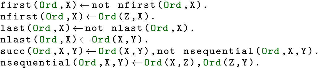
It is easy to check that this program is a Stratified Linear Higher-Order Datalog $^\neg$
one.
$^\neg$
one.
Example 3. The Graph Recoloring problem asks whether it is possible to transform one valid vertex coloring of a graph into another valid target coloring by changing the color of exactly one vertex at a time. A crucial constraint is that every intermediate step in this sequence must also be a valid coloring (i.e., no two adjacent vertices may share the same color). Because the configuration space of all possible colorings for a graph is finite but exponentially large, searching for a path between two colorings is an archetypal reachability problem. Bonsma and Cereceda (Reference Bonsma and Cereceda2009) prove that deciding whether such a reconfiguration path exists between two colorings is a PSPACE-complete problem.
The following program solves the Graph Recoloring problem. In this program, a graph is defined by the predicates node and edge. A specific coloring of a graph is represented as a binary relation C, where the atom C(X,Col) indicates that node X is assigned color Col. The target coloring is represented by the relation target_coloring.
Before we can determine if a graph can be recolored, we must first define what constitutes a structurally sound, valid coloring. We do this by defining the conditions that make a coloring invalid, and then concluding that a coloring is valid if none of those conditions apply.

The invalid_coloring predicate captures the three ways a coloring attempt can fail: (a) two distinct nodes connected by an edge share the exact same color; (b) a single node is simultaneously assigned two different colors, and (c) a node in the graph does not have any color assigned to it at all.
A valid recoloring sequence requires changing the color of exactly one node at a time, ensuring that every intermediate state remains a valid graph coloring. Finally, the program must check if this sequence of transitions successfully reaches the target_coloring.

The valid_step(C1,C2) enforces the rules that both the starting coloring (C1) and resulting coloring (C2) are valid colorings, and exactly one node changes color. The latter is checked by the predicate one_diff. Both one_diff and the auxiliary predicate eq that checks whether two binary relations are equal can be defined as follows.

It is easy to verify that the above program is stratified: every non-recursive predicate in the program can be assigned on its own stratum, and the sole recursive predicate, recolorable, depends only positively on itself, therefore preserving this hierarchy. Furthermore, the program maintains the linearity within every stratum. The only interesting case is the recursive rule of predicate recolorable, where the body contains exactly one predicate from the same stratum that is recolorable itself. This predicate appears exactly once, alongside valid_step which resides in a lower stratum.
Languages such as Higher-Order Datalog $^\neg$
, are usually referred as formal query languages. A program in our language can be considered to compute a query in the following sense: a first-order predicate, like e in Example2, will be called an input predicate and its denotation (as a set of ground atoms) constitutes what is called the input database, usually denoted by
$^\neg$
, are usually referred as formal query languages. A program in our language can be considered to compute a query in the following sense: a first-order predicate, like e in Example2, will be called an input predicate and its denotation (as a set of ground atoms) constitutes what is called the input database, usually denoted by $D_{in}$
; a first-order predicate like hamilton in Example2, will be an output one and its denotation constitutes the output database, usually denoted by
$D_{in}$
; a first-order predicate like hamilton in Example2, will be an output one and its denotation constitutes the output database, usually denoted by $D_{out}$
.
$D_{out}$
.
Formally, a database schema $\sigma$
is a finite set of first-order predicate symbols with associated arities. A database over a schema
$\sigma$
is a finite set of first-order predicate symbols with associated arities. A database over a schema $\sigma$
is a finite set of ground atoms whose predicate symbols belong to
$\sigma$
is a finite set of ground atoms whose predicate symbols belong to $\sigma$
. A query is a mapping from databases over a schema
$\sigma$
. A query is a mapping from databases over a schema $\sigma _1$
to databases over a schema
$\sigma _1$
to databases over a schema $\sigma _2$
. A program
$\sigma _2$
. A program $\mathsf{P}$
can be seen as a query
$\mathsf{P}$
can be seen as a query ${\mathcal{Q}}_{\mathsf{P}}$
such that
${\mathcal{Q}}_{\mathsf{P}}$
such that $D_{out} = {\mathcal{Q}}_{\mathsf{P}}(D_{in})$
. We are interested in queries that are generic (Immerman Reference Immerman1986), that is queries that do not depend on the names of the individual constants in the input database. Given a fragment of our language, we are interested in the expressive power of the fragment, namely the set of queries that can be defined by programs of the fragment. We want to demonstrate that the fragment captures a complexity class
$D_{out} = {\mathcal{Q}}_{\mathsf{P}}(D_{in})$
. We are interested in queries that are generic (Immerman Reference Immerman1986), that is queries that do not depend on the names of the individual constants in the input database. Given a fragment of our language, we are interested in the expressive power of the fragment, namely the set of queries that can be defined by programs of the fragment. We want to demonstrate that the fragment captures a complexity class $\mathcal{C}$
, that is it can express exactly all the queries whose evaluation complexity belongs to
$\mathcal{C}$
, that is it can express exactly all the queries whose evaluation complexity belongs to $\mathcal{C}$
. Evaluation complexity is the complexity of checking whether a given atom belongs to the output database.
$\mathcal{C}$
. Evaluation complexity is the complexity of checking whether a given atom belongs to the output database.
4 Simulation of space-bounded turing machines
In this section, we demonstrate how any query that belongs to $(k-1)$
-EXPSPACE (
$(k-1)$
-EXPSPACE ( $k\geq 1$
), can be expressed by a
$k\geq 1$
), can be expressed by a $(k+1)$
-order Stratified Linear Datalog
$(k+1)$
-order Stratified Linear Datalog $^\neg$
program. Without loss of generality, we assume that the output schema of the query consists of a single output predicate, since every query can be decomposed into multiple queries of this form. By definition, since the query belongs to
$^\neg$
program. Without loss of generality, we assume that the output schema of the query consists of a single output predicate, since every query can be decomposed into multiple queries of this form. By definition, since the query belongs to $(k-1)$
-EXPSPACE, there exists a Turing machine that given on its tape an input database under some sensible encoding, decides whether a tuple belongs to the output relation of the query; furthermore, it does so using at most
$(k-1)$
-EXPSPACE, there exists a Turing machine that given on its tape an input database under some sensible encoding, decides whether a tuple belongs to the output relation of the query; furthermore, it does so using at most $\textrm {exp}_{k-1}(n^d)$
tape cells, where
$\textrm {exp}_{k-1}(n^d)$
tape cells, where $n$
is the number of constant symbols in the input database and
$n$
is the number of constant symbols in the input database and $d$
is some sufficiently large constant (assume
$d$
is some sufficiently large constant (assume $\textrm {exp}_{-1}(x) = \lceil \log x \rceil$
). We formalize this result as follows:
$\textrm {exp}_{-1}(x) = \lceil \log x \rceil$
). We formalize this result as follows:
Theorem 4.1. Every query in $(k-1)$
-EXPSPACE (
$(k-1)$
-EXPSPACE ( $k \geq 1$
) can be expressed by a
$k \geq 1$
) can be expressed by a $(k+1)$
-order Stratified Linear Datalog
$(k+1)$
-order Stratified Linear Datalog $^\neg$
program.
$^\neg$
program.
To establish this theorem, we construct a simulation of an arbitrary space-bounded Turing machine using Stratified Linear Higher-Order Datalog $^\neg$
. Our simulation strategy is to represent the tape as a function that maps an address of a tape cell to a symbol of the alphabet of the machine. To uniquely identify cells on an exponentially large tape, we require a mechanism to represent and manipulate equally large natural numbers as tape indices. We utilize higher-order variables to represent numbers; specifically, we construct “counting modules” where a predicate of order
$^\neg$
. Our simulation strategy is to represent the tape as a function that maps an address of a tape cell to a symbol of the alphabet of the machine. To uniquely identify cells on an exponentially large tape, we require a mechanism to represent and manipulate equally large natural numbers as tape indices. We utilize higher-order variables to represent numbers; specifically, we construct “counting modules” where a predicate of order $k$
can represent a number up to
$k$
can represent a number up to $\textrm {exp}_{k}(n^{d+1})-1$
for some fixed
$\textrm {exp}_{k}(n^{d+1})-1$
for some fixed $d$
. We assume that the alphabet of the machine is the set of three symbols
$d$
. We assume that the alphabet of the machine is the set of three symbols $\{0, 1, \square \}$
where
$\{0, 1, \square \}$
where $\square$
denotes the blank symbol. We decompose the tape into two disjoint higher-order predicates. One predicate tracks the set of addresses where the tape bit is set to
$\square$
denotes the blank symbol. We decompose the tape into two disjoint higher-order predicates. One predicate tracks the set of addresses where the tape bit is set to $1$
, while the other tracks addresses where the bit is set to
$1$
, while the other tracks addresses where the bit is set to $0$
. Any address not present in either set is implicitly treated as containing the
$0$
. Any address not present in either set is implicitly treated as containing the $\square$
symbol.
$\square$
symbol.
4.1 Representation of numbers
Indexing an exponentially large tape requires a mechanism for representing exponentially large natural numbers. We adopt the representation scheme described by Charalambidis et al. (Reference Charalambidis, Kostopoulos, Nomikos and Rondogiannis2025) where predicates of order $k$
are used to represent numbers of magnitude
$k$
are used to represent numbers of magnitude $\textrm {exp}_{k}(n^d)$
. As we will demonstrate later, this representation constitutes a Stratified Linear Higher-Order Datalog program.
$\textrm {exp}_{k}(n^d)$
. As we will demonstrate later, this representation constitutes a Stratified Linear Higher-Order Datalog program.
Natural numbers up to $n^{d+1}-1$
are represented using tuples of individual constants with a fixed length of
$n^{d+1}-1$
are represented using tuples of individual constants with a fixed length of $d+1$
, where
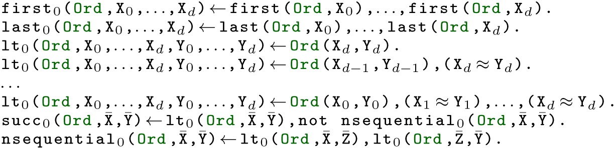
$d+1$
, where $d$
is an arbitrary but fixed natural number. The following predicates define the “first” and “last” of such numbers (denoted by first
$d$
is an arbitrary but fixed natural number. The following predicates define the “first” and “last” of such numbers (denoted by first ${}_{0}$
and last
${}_{0}$
and last ${}_{0}$
) and the “less-than” and “successor” relations on them (denoted by lt
${}_{0}$
) and the “less-than” and “successor” relations on them (denoted by lt ${}_{0}$
and succ
${}_{0}$
and succ ${}_{0}$
). Notice that the following definitions rely on the first and last predicates defined in Example2.
${}_{0}$
). Notice that the following definitions rely on the first and last predicates defined in Example2.
We extend this system to represent “exponentially-big” numbers using higher-order relations. Let $N_0 = n^{d+1} - 1$
be the largest number that can be represented by
$N_0 = n^{d+1} - 1$
be the largest number that can be represented by $(d+1)$
-tuples of individual constants and for
$(d+1)$
-tuples of individual constants and for $k \geq 1$
, let
$k \geq 1$
, let $N_k$
be the largest number that can be represented by using
$N_k$
be the largest number that can be represented by using $k$
-order relations. We can exponentially increase the numbers up to the number
$k$
-order relations. We can exponentially increase the numbers up to the number $N_{k+1} = \textrm {exp}_1(N_k + 1)-1$
by using
$N_{k+1} = \textrm {exp}_1(N_k + 1)-1$
by using $(k+1)$
-order relations. Generally, it holds that
$(k+1)$
-order relations. Generally, it holds that $N_{k} = \textrm {exp}_{k}(n^{d+1})-1$
.
$N_{k} = \textrm {exp}_{k}(n^{d+1})-1$
.
If the $k$
-order relations representing numbers up to
$k$
-order relations representing numbers up to $N_k$
are of type
$N_k$
are of type $\rho$
, then it suffices to use higher-order relations of type
$\rho$
, then it suffices to use higher-order relations of type $\rho \rightarrow o$
in order to represent numbers up to
$\rho \rightarrow o$
in order to represent numbers up to $N_{k+1}$
. This is essentially a binary representation where the lower order numbers denote bit positions. Formally, let Z be a
$N_{k+1}$
. This is essentially a binary representation where the lower order numbers denote bit positions. Formally, let Z be a $(k+1)$
-order element and
$(k+1)$
-order element and ${\tt R}_0,\ldots ,{\tt R}_{N_k}$
be the ordering of the elements that represent numbers in the previous counting module. Let
${\tt R}_0,\ldots ,{\tt R}_{N_k}$
be the ordering of the elements that represent numbers in the previous counting module. Let $f$
be the function mapping
$f$
be the function mapping $\mathit{true}$
to
$\mathit{true}$
to $1$
and
$1$
and $\mathit{false}$
to
$\mathit{false}$
to $0$
. Then, we have
$0$
. Then, we have $num({\tt Z}) = f({\tt Z(R}_{0})) + f({\tt Z(R}_{1})) \cdot 2 + \cdots + f({\tt Z(R}_{N_k}))\cdot 2^{N_k}$
. We begin with predicates testing for the first and the last number.
$num({\tt Z}) = f({\tt Z(R}_{0})) + f({\tt Z(R}_{1})) \cdot 2 + \cdots + f({\tt Z(R}_{N_k}))\cdot 2^{N_k}$
. We begin with predicates testing for the first and the last number.

The following definitions describe the “less than” relation between two elements that represent numbers. We examine if a number N is less than M by comparing the two numbers bit by bit in their binary representation. The successor of a number is defined with the use of less-than.

For the case where $k=0$
the variables X and Y in the code above must be substituted with the tuple vectors
$k=0$
the variables X and Y in the code above must be substituted with the tuple vectors $\bar {\tt X}$
and
$\bar {\tt X}$
and $\bar {\tt Y}$
.
$\bar {\tt Y}$
.
It is straightforward to verify that the counting modules of any order $k\geq 0$
constitutes a stratified linear program. First, notice that there is a strict dependency on the order of the predicates: predicates of order
$k\geq 0$
constitutes a stratified linear program. First, notice that there is a strict dependency on the order of the predicates: predicates of order $k+1$
depend either on other predicates of order
$k+1$
depend either on other predicates of order $k+1$
or on predicates of strictly lower order. Consequently, all predicates of order
$k+1$
or on predicates of strictly lower order. Consequently, all predicates of order $k$
can be assigned to strata strictly lower than those of order
$k$
can be assigned to strata strictly lower than those of order $k+1$
. Second, within the specific order
$k+1$
. Second, within the specific order $k+1$
we impose a stratification function
$k+1$
we impose a stratification function $S$
as:
$S$
as:
 \begin{equation*}S(\mathtt {succ}_{k+1})\gt S(\mathtt {nsequential}_{k+1})\gt S(\mathtt {lt}_{k+1})\gt S(\mathtt {bit}_{k+1})\end{equation*}
Predicates such as first ${}_{k+1}$
and last
${}_{k+1}$
and last ${}_{k + 1}$
can be placed at the lowest stratum of the
${}_{k + 1}$
can be placed at the lowest stratum of the $(k+1)$
-order predicates. Finally, regarding linearity, the only recursive definition at order
$(k+1)$
-order predicates. Finally, regarding linearity, the only recursive definition at order $k+1$
is the bit
$k+1$
is the bit ${}_{k + 1}$
. By inspection of its rules, we observe that it depends on exactly one literal of itself, satisfying the linearity condition.
${}_{k + 1}$
. By inspection of its rules, we observe that it depends on exactly one literal of itself, satisfying the linearity condition.
4.2 The simulation of the turing machine
We now demonstrate how any query that belongs to $(k-1)$
-EXPSPACE (
$(k-1)$
-EXPSPACE ( $k\geq 1$
), can be expressed by a stratified linear
$k\geq 1$
), can be expressed by a stratified linear $(k+1)$
-order Datalog
$(k+1)$
-order Datalog $^\neg$
program. The simulation is markedly different from that of Charalambidis et al. (Reference Charalambidis, Kostopoulos, Nomikos and Rondogiannis2025) which was easier since it could utilize the full power of unrestricted Higher-Order Datalog
$^\neg$
program. The simulation is markedly different from that of Charalambidis et al. (Reference Charalambidis, Kostopoulos, Nomikos and Rondogiannis2025) which was easier since it could utilize the full power of unrestricted Higher-Order Datalog $^\neg$
.
$^\neg$
.
Before presenting the simulation of the Turing machine $M$
, we mention certain simplifying assumptions, which do not affect the generality of the subsequent results.
$M$
, we mention certain simplifying assumptions, which do not affect the generality of the subsequent results.
-
• The input database consists of a single binary relation in and the output database is also a single binary relation out. In the following, the number of constants in the input database is denoted by
$n$
. -
• The alphabet of
$M$
that will be simulated is
$\Sigma =\{0,1,\Box \}$
.
$M$
expects the input relation in as the standard binary encoding of a graph, which is based on the ordering of the individual constants, in the first
$n^2$
cells of its tape. For example, if the pair
$(x,y)$
belongs to in, then the tape of
$M$
contains a “1” at cell position
$num(x)+num(y) \cdot n$
, otherwise it contains “0”. -
•
$M$
decides whether a tuple
$(a,b)$
belongs to the output relation out. The next
$n^2$
cells of its tape are used to encode
$(a,b)$
. All these cells contain the symbol “0”, except for the cell at position
$num(a)+num(b) \cdot n+n^2$
which contains “1”. -
•
$M$
reaches its accepting state
$yes$
if and only if the tuple
$(a,b)$
belongs to the output relation out.








We assume a Turing machine $M$
of three symbols
$M$
of three symbols $\Sigma =\{0,1,\Box \}$
. By convention, we use two predicates input
$\Sigma =\{0,1,\Box \}$
. By convention, we use two predicates input ${}_{0}$
and input
${}_{0}$
and input ${}_{1}$
to encode the input tape of
${}_{1}$
to encode the input tape of $M$
. Specifically, input
$M$
. Specifically, input ${}_{0}$
holds at position
${}_{0}$
holds at position $\bar {\tt X}$
iff the tape contains “0” at
$\bar {\tt X}$
iff the tape contains “0” at $\bar {\tt X}$
, input
$\bar {\tt X}$
, input ${}_{1}$
holds at
${}_{1}$
holds at $\bar {\tt X}$
iff the tape contains “1” at
$\bar {\tt X}$
iff the tape contains “1” at $\bar {\tt X}$
, and the tape contains the blank symbol “
$\bar {\tt X}$
, and the tape contains the blank symbol “ $\Box$
” iff neither holds. By construction below, the two predicates are disjoint.
$\Box$
” iff neither holds. By construction below, the two predicates are disjoint.
The following two predicates encode the binary input relation in and the tuple $(a,b)$
as a binary string. In the following rules, we pad the binary input relation with fixed constants to form
$(a,b)$
as a binary string. In the following rules, we pad the binary input relation with fixed constants to form $(d+1)$
-arity tuples representing valid tape addresses.
$(d+1)$
-arity tuples representing valid tape addresses.

We also need a higher-order predicate to lift the tuple representation of numbers to the $(k-1)$
-order numbering notation in order to transfer the input of the tape from a zero order relation to a
$(k-1)$
-order numbering notation in order to transfer the input of the tape from a zero order relation to a $(k-1)$
-order relation. The predicate lift
$(k-1)$
-order relation. The predicate lift ${}_{k-1} (\textcolor {green}{\mathtt {Ord}}$
,
${}_{k-1} (\textcolor {green}{\mathtt {Ord}}$
, $\bar{\texttt{X}}$
, M) transforms the number represented by the tuple
$\bar{\texttt{X}}$
, M) transforms the number represented by the tuple $\bar {\tt X}$
in the zero-order notation to the same number M in the
$\bar {\tt X}$
in the zero-order notation to the same number M in the $(k-1)$
-order notation.
$(k-1)$
-order notation.

We then define the two predicates symbol ${}_0$
and symbol
${}_0$
and symbol ${}_1$
that are the
${}_1$
that are the $(k-1)$
-order analogues of the input predicates input
$(k-1)$
-order analogues of the input predicates input ${}_0$
and input
${}_0$
and input ${}_1$
.
${}_1$
.

With the input prepared, we model the Turing machine’s execution as a reachability analysis on the graph of configurations. We adopt a forward approach: a configuration is valid if it leads to an accepting state.
Consider the transition $(s,\texttt {0})\longrightarrow (s',\texttt {1},\text{R})$
which reads: “if the current state of the machine is
$(s,\texttt {0})\longrightarrow (s',\texttt {1},\text{R})$
which reads: “if the current state of the machine is $s$
and its cursor reads the symbol “0”, then the machine changes its state to
$s$
and its cursor reads the symbol “0”, then the machine changes its state to $s'$
, it writes “1” on the current cursor position onto the tape and then moves the cursor to the right.” We encode this logic such that the validity of the current state
$s'$
, it writes “1” on the current cursor position onto the tape and then moves the cursor to the right.” We encode this logic such that the validity of the current state $s$
depends on the validity of the successor state
$s$
depends on the validity of the successor state $s'$
.
$s'$
.

This rule asserts that if the machine successfully accepts starting from state $s'$
, it also accepts starting from state
$s'$
, it also accepts starting from state $s$
. The successor state
$s$
. The successor state $s'$
reflects the updated tape and the cursor moved to the right or left by enforcing succ
$s'$
reflects the updated tape and the cursor moved to the right or left by enforcing succ
 , P, P ${}^{\prime}$
) or succ
${}^{\prime}$
) or succ
 , P
′
, P) respectively.
, P
′
, P) respectively.
The transition rules above rely on the ability to modify the tape. Recall that the tape is encoded by the two disjoint relations Tp ${}_1$
and Tp
${}_1$
and Tp ${}_0$
, holding the positions where the tape contains “1” and “0” respectively. Writing the symbol “
${}_0$
, holding the positions where the tape contains “1” and “0” respectively. Writing the symbol “ $b$
” at position P therefore involves updating both relations: P is added to Tp
$b$
” at position P therefore involves updating both relations: P is added to Tp ${}_b$
and removed from the other; for example writing “1” at P puts P into Tp
${}_b$
and removed from the other; for example writing “1” at P puts P into Tp ${}_1$
and removes it from Tp
${}_1$
and removes it from Tp ${}_0$
. We capture these two elementary set operations with the helper predicates flip
${}_0$
. We capture these two elementary set operations with the helper predicates flip ${}_1$
and flip
${}_1$
and flip ${}_0$
, defined as follows:
${}_0$
, defined as follows:

Intuitively, the partial application flip ${}_1$
(Tp,P) denotes the relation
${}_1$
(Tp,P) denotes the relation $\mathtt {Tp}\cup \{\mathtt {P}\}$
, that is Tp extended so that P belongs to it, while flip
$\mathtt {Tp}\cup \{\mathtt {P}\}$
, that is Tp extended so that P belongs to it, while flip ${}_0$
(Tp,P) denotes
${}_0$
(Tp,P) denotes $\mathtt {Tp}\setminus \{\mathtt {P}\}$
, that is Tp with P removed. Writing the symbol “1” at position P is then accomplished by passing flip
$\mathtt {Tp}\setminus \{\mathtt {P}\}$
, that is Tp with P removed. Writing the symbol “1” at position P is then accomplished by passing flip ${}_1$
(Tp
${}_1$
(Tp ${}_1$
,P) and flip
${}_1$
,P) and flip ${}_0$
(Tp
${}_0$
(Tp ${}_0$
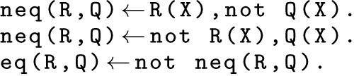
,P) to the recursive call, as in the transition rule above; writing “0” is symmetric, with the roles of the two relations exchanged. Both definitions rely on the auxiliary predicates eq and neq, which check whether two relations (of the same type) are equal or not and are defined as:
${}_0$
,P) to the recursive call, as in the transition rule above; writing “0” is symmetric, with the roles of the two relations exchanged. Both definitions rely on the auxiliary predicates eq and neq, which check whether two relations (of the same type) are equal or not and are defined as:
The recursion defined in the transition rules must eventually terminate. We ground the simulation by defining the accepting state “yes” as true for any valid tape configuration:

Finally, we start the simulation by querying the initial configuration. The following query checks if the initial state $s_0$
(with the initial cursor position and input symbols) can effectively “reach” the accepting state
$s_0$
(with the initial cursor position and input symbols) can effectively “reach” the accepting state $\mathit{yes}$
via the rules defined above:
$\mathit{yes}$
via the rules defined above:

This means that the query is true if the state ${}_{s_0}$
is true for the initial tape state and with the cursor being at the beginning of the tape which in turn is true if this configuration is reachable by one accepting configuration.
${}_{s_0}$
is true for the initial tape state and with the cursor being at the beginning of the tape which in turn is true if this configuration is reachable by one accepting configuration.
We conclude the construction by verifying that the simulation is a stratified linear program. The core of the simulation lies in the transition rules for the state ${}_{\texttt{s}}$
predicates which form a single stratum of mutually recursive definitions. Crucially, each rule depends recursively on exactly one state
${}_{\texttt{s}}$
predicates which form a single stratum of mutually recursive definitions. Crucially, each rule depends recursively on exactly one state $_{s}$
predicate, satisfying the linearity constraint. All auxiliary predicates, such as succ
$_{s}$
predicate, satisfying the linearity constraint. All auxiliary predicates, such as succ ${}_{k + 1}$
, flip
${}_{k + 1}$
, flip ${}_0$
and flip
${}_0$
and flip ${}_1$
are defined without dependence on any state
${}_1$
are defined without dependence on any state ${}_s$
predicate allowing them to be placed on lower strata.
${}_s$
predicate allowing them to be placed on lower strata.
5 Space-efficient computation of stratified linear higher-order programs
Using a simple-minded bottom-up approach to compute the answer to a query, would require space tower-exponential in the order of the given program. To capture the precise space complexity of Stratified Linear Higher-Order Datalog $^\neg$
, we must avoid producing and storing the entire model of a program. In this section, we present a space-efficient computation that proceeds in a top-down fashion. We demonstrate that for a
$^\neg$
, we must avoid producing and storing the entire model of a program. In this section, we present a space-efficient computation that proceeds in a top-down fashion. We demonstrate that for a $(k+1)$
-order Stratified Linear Datalog
$(k+1)$
-order Stratified Linear Datalog $^\neg$
program, a query
$^\neg$
program, a query $p(\bar {d})$
can be evaluated using memory bounded by
$p(\bar {d})$
can be evaluated using memory bounded by $(k-1)-\textsf {EXPSPACE}$
. We formalize this result in the following theorem:
$(k-1)-\textsf {EXPSPACE}$
. We formalize this result in the following theorem:
Theorem 5.1. Let $\mathsf{P}$
be a Stratified Linear
$\mathsf{P}$
be a Stratified Linear $(k+1)$
-Order Datalog
$(k+1)$
-Order Datalog $^\neg$
program that defines a query. Then, there exists a deterministic Turing machine that takes as input an encoding of a database
$^\neg$
program that defines a query. Then, there exists a deterministic Turing machine that takes as input an encoding of a database $D$
that uses
$D$
that uses $n$
individual constant symbols and a ground atom
$n$
individual constant symbols and a ground atom $p(\bar {a})$
, where
$p(\bar {a})$
, where $p$
is a predicate constant of
$p$
is a predicate constant of $\mathsf{P}$
and
$\mathsf{P}$
and $\bar {a}$
is a tuple of these individual constants, and decides whether
$\bar {a}$
is a tuple of these individual constants, and decides whether $p(\bar {a}) \in {\mathcal{Q}}_{\mathsf{P}}(D)$
, while using at most
$p(\bar {a}) \in {\mathcal{Q}}_{\mathsf{P}}(D)$
, while using at most $\textrm {exp}_{k-1}(n^d)$
tape cells, for some constant
$\textrm {exp}_{k-1}(n^d)$
tape cells, for some constant $d$
.
$d$
.
Our evaluation strategy relies on the stratified and linear nature of the program. The meaning of a stratified $(k+1)$
-order Datalog program can be computed stratum by stratum, starting from the lowest and moving upwards. To evaluate queries in the
$(k+1)$
-order Datalog program can be computed stratum by stratum, starting from the lowest and moving upwards. To evaluate queries in the $(m+1)$
-th stratum, we employ two routines:
$(m+1)$
-th stratum, we employ two routines:
-
• A query machine for the
$(m+1)$
-th stratum that decides the truth of an atom
$(\mathsf{p}\,d_1\cdots d_n)$
where
$\mathsf{p}$
is a predicate belonging to the
$(m+1)$
-th stratum and the
$d_i$
are representations of expression values (see explanation later in the section). For the initial query, the
$d_i$
are just individual constants. -
• An expression evaluator for the
$m$
-th stratum that, given a variable assignment, computes the value of a given expression
$\mathsf{E}$
of a type with order at most
$k$
, with the restriction that
$\mathsf{E}$
is formed using predicates solely from the first
$m$
strata.


The query machine for the $(m+1)$
-th stratum requires that the corresponding expression evaluator for the
$(m+1)$
-th stratum requires that the corresponding expression evaluator for the $m$
-th stratum is already defined since it invokes it. On the other hand, the evaluator routine for the
$m$
-th stratum is already defined since it invokes it. On the other hand, the evaluator routine for the $m$
-th stratum requires the query routine for any stratum
$m$
-th stratum requires the query routine for any stratum $m' \leq m$
to be defined. If we take the first stratum to be the set of the (first-order) input predicates supplied from the database in the form of facts, then for
$m' \leq m$
to be defined. If we take the first stratum to be the set of the (first-order) input predicates supplied from the database in the form of facts, then for $m=0$
these routines are easily defined and thus omitted.
$m=0$
these routines are easily defined and thus omitted.
We now define the above routines at a high level of abstraction. A more formal presentation and the corresponding correctness proofs, are given in the supplementary material.
Query machine for the $(m+1)$
-th stratum:
$(m+1)$
-th stratum:
-
1. Start with the atom
$(\mathsf{p}\,d_1\cdots d_n)$
written on the tape, where the
$d_i$
are representations of expression values, that is a string that describes the value (e.g., a relation can be represented as a string listing all tuples in some predetermined order). -
2. Non-deterministically select a rule
$\mathsf{p}\ \mathsf{R}_1 \cdots \mathsf{R}_n \leftarrow \mathsf{L}_1, \ldots , \mathsf{L}_r$
from
$\mathsf{P}$
for predicate
$\mathsf{p}$
and guess a valid assignment for the rule’s variables such that
$d_i$
is assigned to
$\mathsf{R}_i$
for all
$i \in \{ 1,\ldots , n\}$
. -
3. Iterate through the literals
$\mathsf{L}_i$
in the rule body:-
• If
$\mathsf{L}_i$
is a negative literal then
$\mathsf{L}_i$
is of the form
$({\tt not}\ \mathsf{E})$
. Invoke the expression evaluator for the
$m$
-th stratum, passing as parameter the guessed variable assignment, to compute
$\mathsf{E}$
. If the evaluation returns
$\mathit{true}$
, then reject, otherwise proceed to the next literal. -
• If
$\mathsf{L}_i$
is a positive literal and there is no predicate in
$\mathsf{L}_i$
from the
$(m+1)$
-th stratum, then invoke the expression evaluator for the
$m$
-th stratum, passing as parameter the guessed variable assignment, to compute
$\mathsf{L}_i$
. If the evaluation returns
$\mathit{true}$
, then proceed to the next literal, otherwise reject. -
• If there is a predicate in
$\mathsf{L}_i$
from the
$(m+1)$
-th stratum, then this is the unique recursive literal
$\mathsf{q}\ \mathsf{E}_1 \cdots \mathsf{E}_t$
implied by linearity. Every
$\mathsf{E}_j$
is of order at most
$k$
and includes predicates from the first
$m$
strata. Iterate through
$\mathsf{E}_1,\ldots ,\mathsf{E}_t$
invoking each time the evaluator for the
$m$
-th stratum, passing as parameter the guessed variable assignment, to compute each
$ \mathsf{E}_j$
and store the representations
$d'_1,\ldots ,d'_t$
. Construct a new ground atom
$\mathsf{q}\,d'_1 \cdots d'_t$
.
-
-
4. If all literals
$\mathsf{L}_i$
evaluate to
$\mathit{true}$
without encountering a recursive literal, then accept. -
5. If one of the literals
$\mathsf{L}_i$
is a recursive one, overwrite the current goal with
$\mathsf{q}\,d'_1 \cdots d'_t$
and loop back to Step 2.





Note that the aforementioned query machine is nondeterministic and may contain computational paths that do not terminate (e.g., consider the rule p $\leftarrow$
p). This machine is not technically a decider of whether
$\leftarrow$
p). This machine is not technically a decider of whether $(\mathsf{p}\,d_1\cdots d_n)$
is true or not. However, for machines that are space bounded (more specifically by a space constructible function
$(\mathsf{p}\,d_1\cdots d_n)$
is true or not. However, for machines that are space bounded (more specifically by a space constructible function $f(n)$
(Sipser, Reference Sipser2012)) there exists a corresponding nondeterministic Turing machine where every computational path terminates. By Savitch (Reference Savitch1970), there also exists a deterministic machine that computes the same query within the same space complexity class. In the following when we refer to the query machine we mean the deterministic version.
$f(n)$
(Sipser, Reference Sipser2012)) there exists a corresponding nondeterministic Turing machine where every computational path terminates. By Savitch (Reference Savitch1970), there also exists a deterministic machine that computes the same query within the same space complexity class. In the following when we refer to the query machine we mean the deterministic version.
We now define the expression evaluator for the $m$
-th stratum. Let
$m$
-th stratum. Let $\mathsf{E}$
be an expression of order at most
$\mathsf{E}$
be an expression of order at most $k$
that includes predicates from the first
$k$
that includes predicates from the first $m$
strata. The expression evaluator makes calls to query machines in order to construct a representation of the expression’s value.
$m$
strata. The expression evaluator makes calls to query machines in order to construct a representation of the expression’s value.
Expression evaluator for the $m$
-th stratum:
$m$
-th stratum:
-
• If the expression
$\mathsf{E}$
is an individual constant, then return the constant. -
• If the expression
$\mathsf{E}$
is of the form
$(\mathsf{q}\ \mathsf{E}_1\cdots \mathsf{E}_t)$
where
$\mathsf{q}$
belongs to the
$m'$
-th stratum,
$m' \leq m$
, and its type is
$\rho _1 \to \ldots \to \rho _t \to \cdots \to \rho _{t'} \to o$
. Then:



-
1. Evaluate the expressions
$\mathsf{E}_1, \ldots , \mathsf{E}_t$
sequentially to obtain and store their representations
$d_1,\ldots ,d_t$
. This is performed by calling the evaluator recursively for each subexpression. -
2. To determine the representation of the result, the machine enumerates all possible tuples
$d_{t+1}, \ldots , d_{t'}$
of representations regarding the remaining arguments. For each tuple, it invokes the query machine for the
$m'$
-th stratum with the goal
$(\mathsf{q}\, d_1 \cdots d_{t}\, d_{t+1} \cdots d_{t'})$
.



-
• If the expression
$\mathsf{E}$
is of the form
$(\mathsf{X}\ \mathsf{E}_1\cdots \mathsf{E}_t)$
where
$\mathsf{X}$
is a variable (of order at most
$k$
) then it evaluates the expressions
$\mathsf{E}_1, \ldots , \mathsf{E}_t$
to obtain and store the representation of their values
$d_1,\ldots ,d_t$
, and then uses the variable assignment of
$\mathsf{X}$
to compute the representation of the value of the application.


The last two bullets implicitly handle the cases where there are zero arguments.
We now briefly comment on the space complexity; the full and precise arguments are given in the supplementary material . The query machine’s space complexity depends on storing the current goal, guessing variable assignments, and evaluating lower-strata subroutines. For a $(k+1)$
-order program, arguments are at most order
$(k+1)$
-order program, arguments are at most order $k$
, belonging to a domain of size
$k$
, belonging to a domain of size $\textrm {exp}_k(poly(n))$
. Representing these arguments requires unique identifiers of logarithmic size, that is
$\textrm {exp}_k(poly(n))$
. Representing these arguments requires unique identifiers of logarithmic size, that is $\textrm {exp}_{k-1}(poly(n))$
bits. Therefore, storing the current goal and variable assignments takes
$\textrm {exp}_{k-1}(poly(n))$
bits. Therefore, storing the current goal and variable assignments takes $\textrm {exp}_{k-1}(poly(n))$
space. Crucially, program linearity allows the machine to overwrite the current goal during recursion, preventing depth-related memory blow-up. Furthermore, lower-strata expressions are evaluated sequentially (reusing memory), and since the number of strata is a fixed constant independent of the input size
$\textrm {exp}_{k-1}(poly(n))$
space. Crucially, program linearity allows the machine to overwrite the current goal during recursion, preventing depth-related memory blow-up. Furthermore, lower-strata expressions are evaluated sequentially (reusing memory), and since the number of strata is a fixed constant independent of the input size $n$
, the call stack depth is strictly bounded. Consequently, the overall space complexity remains
$n$
, the call stack depth is strictly bounded. Consequently, the overall space complexity remains $\textrm {exp}_{k-1}(poly(n))$
.
$\textrm {exp}_{k-1}(poly(n))$
.
6 Future work: Implementation of 2nd-order Stratified Linear Datalog
$^\neg$

The space complexity results described in this paper are not merely theoretical; they provide the foundation for a practical implementation of the 2nd order fragment of Stratified Linear Datalog $^\neg$
. By capturing PSPACE, this fragment addresses many problems that remain out of reach for traditional ASP systems.
$^\neg$
. By capturing PSPACE, this fragment addresses many problems that remain out of reach for traditional ASP systems.
The key idea behind our implementation is to compile any given 2nd order Stratified Linear Datalog $^\neg$
program and user query into a Quantified Boolean Formula (QBF). We can then use existing, efficient QBF solvers to evaluate the resulting formula and return answers to the initial query. Because evaluating QBFs is the canonical PSPACE-complete problem (Sipser Reference Sipser2012), this translation offers a direct and highly feasible approach to implementing our source language.
$^\neg$
program and user query into a Quantified Boolean Formula (QBF). We can then use existing, efficient QBF solvers to evaluate the resulting formula and return answers to the initial query. Because evaluating QBFs is the canonical PSPACE-complete problem (Sipser Reference Sipser2012), this translation offers a direct and highly feasible approach to implementing our source language.
Due to space limitations, the remainder of this section provides only a high-level overview of this translation, leaving the formal generalization of this technique to a future paper.
The space-efficient computation described in Section 5 models evaluation as a top-down procedure that avoids materializing the full program interpretation. We can conceptualize this evaluation as a reachability problem within a configuration graph. In the first-order setting, linearity implies that the evaluation engine only needs to store the current state of the computation (which is a classical Datalog atom). In the 2nd-order case, the active computation is, in general, a first-order relation. For an input database with a domain of size $n$
, a first-order relation of arity
$n$
, a first-order relation of arity $d$
can be represented by a truth assignment to
$d$
can be represented by a truth assignment to $O(n^d)$
boolean variables. Therefore, a single recursive step in a 2nd-order Stratified Linear Datalog
$O(n^d)$
boolean variables. Therefore, a single recursive step in a 2nd-order Stratified Linear Datalog $^\neg$
program represents a transition from one boolean configuration to another. Because the program is linear, meaning there exists at most one predicate constant in the body from the same stratum, the core query evaluation simply asks whether there is a valid logical path from an initial configuration to an accepting configuration.
$^\neg$
program represents a transition from one boolean configuration to another. Because the program is linear, meaning there exists at most one predicate constant in the body from the same stratum, the core query evaluation simply asks whether there is a valid logical path from an initial configuration to an accepting configuration.
The transformation to QBF relies on encoding these configurations as boolean vectors and capturing the linear recursion using a reachability formula. Let a variable $\mathsf{X}$
representing a first-order relation be encoded as a vector of boolean variables
$\mathsf{X}$
representing a first-order relation be encoded as a vector of boolean variables $\vec {x}$
of length
$\vec {x}$
of length $n^d$
. The linear recursive rules of the current stratum, along with any non-recursive rules or sequences of rules from strictly lower strata they depend on, can be compiled into a quantifier-free boolean formula
$n^d$
. The linear recursive rules of the current stratum, along with any non-recursive rules or sequences of rules from strictly lower strata they depend on, can be compiled into a quantifier-free boolean formula $T(\vec {x}, \vec {y})$
. This formula evaluates to true if and only if state
$T(\vec {x}, \vec {y})$
. This formula evaluates to true if and only if state $\vec {y}$
can be derived from state
$\vec {y}$
can be derived from state $\vec {x}$
in exactly one step. Because the state space of possible configurations has a size of
$\vec {x}$
in exactly one step. Because the state space of possible configurations has a size of $2^{n^d}$
, a linear query might require up to
$2^{n^d}$
, a linear query might require up to $2^{n^d}$
recursive steps to reach the target state. Unrolling the transition formula
$2^{n^d}$
recursive steps to reach the target state. Unrolling the transition formula $T(\vec {x}, \vec {y})$
exponentially would require exponential space, which contradicts our PSPACE bounds. Fortunately, we can follow the principles of Savitch’s theorem and use the expressive power of universal quantifiers in QBF to compress the path search.
$T(\vec {x}, \vec {y})$
exponentially would require exponential space, which contradicts our PSPACE bounds. Fortunately, we can follow the principles of Savitch’s theorem and use the expressive power of universal quantifiers in QBF to compress the path search.
This translation mechanism offers a practical evaluation pipeline. A compiler can map all first-order variables to boolean vectors, compile the linear recursive rules into the base transition formula $T$
, and generate appropriate quantified reachability formulas based on Savitch’s theorem. The resulting formula can then be evaluated by modern QBF solvers. By avoiding the materialization of the full interpretation, this approach strictly adheres to the space-efficient nature of our fragment and provides a viable implementation pathway for 2nd order Stratified Linear Datalog
$T$
, and generate appropriate quantified reachability formulas based on Savitch’s theorem. The resulting formula can then be evaluated by modern QBF solvers. By avoiding the materialization of the full interpretation, this approach strictly adheres to the space-efficient nature of our fragment and provides a viable implementation pathway for 2nd order Stratified Linear Datalog $^\neg$
programs.
$^\neg$
programs.
As another promising direction for future work, it is worth investigating whether we can relax the stratification constraints by introducing a notion of local stratification for Higher-Order Datalog $^\neg$
. Although our current space complexity arguments rely on a fixed number of strata, we conjecture that if the number of strata are polynomial with respect to the input size, the resulting linear programs would still preserve their space efficiency.
$^\neg$
. Although our current space complexity arguments rely on a fixed number of strata, we conjecture that if the number of strata are polynomial with respect to the input size, the resulting linear programs would still preserve their space efficiency.
Supplementary material
To view supplementary material for this article, please visit https://doi.org/10.1017/S1471068426100593
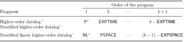
 ∗
∗


 Open access

