

1. INTRODUCTION
Projections of the future evolution of ice sheets such as the Antarctic ice sheet and understanding their evolution is a central subject of ongoing research. One insufficiently represented component in ice-sheet models is the process of calving, i.e. mass loss at the ice front by means of fracture formation leading to the detachments of icebergs. The horizontal extent of ice sheets depends on the evolution of the calving fronts, either at tidewater glaciers or ice shelves. In the present work, we will only consider the latter, which covers 75% of the Antarctic coastline (Rignot and others, Reference Rignot, Jacobs, Mouginot and Scheuchl2013). While evolution equations can be included in numerical models with techniques such as level set methods (Bondzio and others, Reference Bondzio2016), the main problem remains unsolved, namely to determine a physics-based calving law that results in a proper calving rate. Thus far, iceberg drift and melting can be modeled with a high level of accuracy (Rackow and others, Reference Rackow2017), but the production of icebergs still follows empirical or even heuristic approaches. Given that deep water formation in the ocean and climate models is highly sensitive to variations of surface freshwater fluxes (e.g Martin and Adcroft, Reference Martin and Adcroft2010), a physics-based calving law is essential to close the feedback between ocean and cryosphere for global climate projections and studies of potential sea-level rise.
In the current ice-sheet models, calving processes are either replaced by a fixed ice front or parametrized using phenomenological (Alley and others, Reference Alley2008; Amundson and Truffer, Reference Amundson and Truffer2010; Albrecht and others, Reference Albrecht, Martin, Haseloff, Winkelmann and Levermann2011) or even heuristic approaches (Bassis, Reference Bassis2011), cf. the implementations in, for example, the Ice Sheet System Model (ISSM; Larour and others, Reference Larour, Seroussi, Morlighem and Rignot2012), the Parallel Ice Sheet Model (PISM; Bueler and others, Reference Bueler, Lingle and Kallen-Brown2007), the SImulation COde for POLythermal Ice Sheets (SICOPOLIS; Greve and others, Reference Greve, Saito and Abe-Ouchi2011) and Elmer/Ice (Seddik and others, Reference Seddik, Greve, Zwinger, Gillet-Chaulet and Gagliardini2012). Based on observations, Benn and others (Reference Benn, Warren and Mottram2007) classified different calving mechanisms at tidewater glaciers according to individual causes, for example a hydrofracture mechanism of crevasse propagation. The hydrofracture mechanism has been used by Pollard and others (Reference Pollard, DeConto and Alley2015) as a parameterization for ice-cliff failure. Todd and others (Reference Todd2018) extended this approach to three dimensions.
For all approaches, it is necessary to compare available observations of calving to model results that realistically reproduce physical processes in the ice. To obtain a physics-based understanding of calving processes, the short-term elastic response of ice must be considered for various situations such as the changing load condition at the newly formed ice front right after a calving event. Hence, the relevant material characteristics for calving are the short-term elastic and the long-term viscous (flow of ice) behavior leading to a viscoelastic fluid. These material requirements are contained in the description of a Maxwell material (e.g. Christmann, Reference Christmann2017). Other examples in which viscoelasticity is essential are the response of glaciers to tidal forcing (Reeh and others, Reference Reeh, Christensen, Mayer and Olesen2003; Gudmundsson, Reference Gudmundsson2011; Rosier and others, Reference Rosier, Gudmundsson and Green2014) or the potential closing of englacial and subglacial channels with decreasing meltwater supply at the end of the melt season. Furthermore, MacAyeal and others (Reference MacAyeal, Sergienko and Banwell2015) analyzed the filling and draining of supraglacial lakes employing a viscoelastic material model.
Different types of iceberg formation can be defined. These include for instance fragmentation processes in which complete or partial disintegration of ice shelves has been observed at several locations (e.g. Vaughan and others, Reference Vaughan2012; Liu and others, Reference Liu2015). However, these break-up events are widely different to the regular calving of icebergs. Driven by the viscous flow of ice, ice shelves expand over several years to decades during which lateral rifts propagate episodically until an iceberg calves off (Hogg and Gudmundsson, Reference Hogg and Gudmundsson2017). In this case, large icebergs in the order of 10 km2 to 1 000 km2 or even giant icebergs with areas above 1 000 km2 are formed. Occurrence and distribution of rifts thus (at least to a large extent) control the formation of large and giant icebergs. Both fracture fragmentation and the calving that is characterized by the propagation of pre-existing horizontal or vertical rifts (Larour and others, Reference Larour, Rignot and Aubry2004a; Reference Larour, Rignot and Aubry2004b; Plate, Reference Plate2015) are important processes but neither is addressed in the present study.
This study focuses on a second type of calving that occurs for instance at ice shelves with homogeneous, crevasse-free surfaces. Wesche and others (Reference Wesche, Jansen and Dierking2013) classified the surface types of calving fronts in Antarctica. Overall 7.4% of the ice shelves have no surface structures in the vicinity of the calving front, but calving events still happen at these ice shelves. In time intervals between several months to few years, small icebergs in the order of 100 m2 to several km2 detach. This process is called small-scale calving in the present work. Until now, physics-based descriptions of these rather continuous calving processes are missing in ice-sheet models. To consider such a calving behavior, other causes than pre-existing rifts must trigger these events. Furthermore, small-scale calving may also happen in combination with the formation of large tabular icebergs as it is also present at ice shelves containing rifts and crevasses. This combination has been observed for example at Pine Island and Thwaites glaciers (Liu and others, Reference Liu2015) and is of importance for future studies. However, we focus on the investigation of small-scale calving and its mechanisms solely.
A crucial point for the modeling of small-scale calving is to consider the influence of atmospheric and water pressure at the ice front. In this context, several theoretical models tried to explain small iceberg calving (e.g. Reeh, Reference Reeh1968; Reddy and others, Reference Reddy, Bobby, Arockiasamy and Dempster1980; Fastook and Schmidt, Reference Fastook and Schmidt1982; Hughes, Reference Hughes1992). However, no physics-based description was developed to explain the observations of calving at crevasse-free ice tongues. Due to the boundary conditions at the ice front, a bending moment appears which plays a critical role for calving (Todd and others, Reference Todd2018). Bending leads to a deflection of the ice shelf near the terminus and the buoyancy equilibrium is not fulfilled close to the ice front. This boundary disturbance results in a bell-shaped stress distribution (Christmann and others, Reference Christmann, Rückamp, Müller and Humbert2016b). The maximum tensile stress, which may cause calving events, is found at the upper surface. At tidewater glaciers calving is considerably different: bending at the grounding line enforces the propagation of basal crevasses in the upward direction leading to calving (Benn and others, Reference Benn2017). This does not happen at the position of maximum tensile stress. However, in the case of small-scale calving at Antarctic ice shelves, the influence of the grounding line far away from the calving front is insignificant.
Failure concepts such as the hypothesis of critical stress or strain values as calving criteria are discussed in this work. Well established in the literature is a critical stress of σ crit = 330 kPa for consolidated ice (suggested in Pralong, Reference Pralong2005, on the basis of Hayhurst, Reference Hayhurst1972), while other values ranging from 90 kPa to 1 MPa have also been proposed (Vaughan, Reference Vaughan1993; Vaughan and others, Reference Vaughan2012). In contrast to the critical stress, neither a critical strain has ever been observed for polycrystalline ice nor an analogy with metals has been discussed as for the derivation of critical stress by Hayhurst (Reference Hayhurst1972). This does not mean that such a value cannot exist, but further research on this topic is required. In this study, instantaneous cracking through the whole ice thickness is assumed once the critical criterion is reached. This assumption is reasonable as the bending moment of the eccentric water pressure at the ice front promotes calving if a crack is initiated.
In the present work, stress and strain states are examined to understand the essential factors influencing small-scale calving. No explicit calving rate is derived; instead, the impact of two viscoelastic Maxwell material concepts using infinitesimal (linearized strain measure) and finite strain theory are investigated. In the following, we first sketch the theoretical basis of the mathematical models followed by the introduction of the numerical model and the presentation of its usefulness. Subsequently, we discuss the applicability of both approaches to small-scale calving as well as the limitation of the viscoelastic model assuming small strains. To assess the sensitivity to uncertainties in the material parameters or the geometry, parameter studies are performed. Finally, the constant viscosity in the viscoelastic model for finite strains is replaced by the nonlinear Glen-type viscosity and the effect is assessed.
2. CHALLENGES OF VISCOELASTIC MATERIAL MODELING
In constitutive equations of a viscoelastic material model, the stress tensor is not only related to the strain-rate tensor as in the case of a viscous fluid. Additionally, the temporal derivative of the stress tensor is included in the viscoelastic Maxwell model. In order to account not only for stress but also for strain states as possible causes for calving, the unknowns in this work are the displacements. The strain results are mostly disregarded in purely viscous material descriptions of current ice-sheet models since these models solve for velocities.
For small strain values, it is sufficient to use a simplified, linearized strain description based on infinitesimal strain theory. This approach is called throughout this work the small deformation model. However, the strain values in ice shelves caused by the horizontal spreading unavoidably increase with time (Christmann and others, Reference Christmann, Plate, Müller and Humbert2016a). After some time, the strain values do not fulfill the smallness requirement anymore although strain rates may remain small. Consequently, a material model applicable to large and finite strain values is needed. This requires changes in the kinematics and the choice of the configuration. This paper aims to consider the effect of this material approach – hereafter referred to the finite deformation model – on quantities significant for calving. A comparison of numerical results is carried out to show the limitation and shortcomings of the small deformation model.
3. THEORY
Polycrystalline ice reacts in two ways to an external load. An instantaneous elastic deformation occurs and is accompanied by a continuous creep (viscous) deformation. This material behavior can be modeled by a viscoelastic material description of Maxwell type (superposition of elastic and viscous strain). We focus attention on this material law in the present study. It is investigated whether the simplifying assumption of a small deformation model is sufficient to describe calving processes accurately, or whether a more sophisticated finite deformation model is required. As the geometric linearization is accurate only for small deformations, internal and external loads should cause only a limited motion of the considered body.
For the small and the finite deformation approach, the quasi-static local form of the momentum balance reads
 $$ \rm{div}\, {\bisigma}+ {\bi f} = {\bf 0} $$
with the Cauchy stress tensor σ and the volume force f. Gravity is the only external force included in the ice shelf model. Thus, the volume force is given by f = −(ρ ice g)ez, where ρ ice is the ice density, g the acceleration due to gravity and ez = (0, 0, 1)T the upward pointing unit vector. In the following, all equations are first described for the small deformation model before these equations are then extended to the finite deformations framework.
3.1. Small deformation model
The kinematic equation relates the deformation, given by the displacement vector u = (u, v, w)T, to the strains. In the small deformation model the linearized strain tensor ε is given by the symmetric part of the displacement gradient
 $${\bivarepsilon} = {\displaystyle{1} \over {2}} \left(\nabla {\bi u} + \nabla^{T} {\bi u} \right). $$
Equations (1) and (2) are independent of the material under consideration. To close the system of equations a material law is required that relates the kinematic quantities, i.e. strains, to the dynamic quantities, i.e. stress. Material models result from mathematical description that express the characteristic features of a real material in an idealized manner. The material properties are often defined based on an additive decomposition of the stress and strain tensors into a volumetric and a deviatoric part. Here the deviatoric part is denoted by ( · )D = ( · ) − 1/3tr( · )I with the trace operator tr(·) and the second order identity tensor I. In fluid dynamics the thermodynamic pressure p is usually introduced as an additional unknown. Thus the stress is given by σ = −p I + σD. The pressure p is determined by an incompressibility constraint, while σD is given by a material law involving viscosity. The extension of such a viscous flow model to viscoelasticity in order to capture the short-term elastic response of ice is not trivial. In crystalline materials, it is common to assume that the volumetric response is entirely elastic and reversible. Following for example Darby (Reference Darby1976) an elastic isometric/hydrostatic stress is assumed by
 $${\bisigma} = {\underbrace {\left(\lambda + {\displaystyle{2} \over {3}} \mu \right)}_{=K}} {\rm tr} (\bi{\varepsilon}) \bi{I} + {\sigma}^D $$
with the two Lamé constants λ = E ν/[(1 + ν)(1 − 2ν)] and μ = E/[2(1 + ν)], expressed by Young's modulus E and Poisson's ratio ν of an isotropic material. Note that in Eqn. (3) the isometric/hydrostatic stress can be interpreted as a constitutive assumption for the thermodynamic pressure p in laminar flow models. For discussion on this in the small deformation context see Christmann and others (Reference Christmann, Rückamp, Müller and Humbert2016b) and for the finite deformation framework Christmann (Reference Christmann2017). The bulk modulus K describes the resistance of the material against uniform compression. In crystalline materials it is frequently assumed that the volume deformation is linear elastic and not influenced by the deviatoric deformation.
The rate-dependent behavior is introduced only via the deviatoric stress. For a viscoelastic Maxwell material (Fig. 1), the deviatoric stresses in the elastic and viscous elements are equal to the total deviatoric stress σD. The constitutive relation including the viscosity η is given by
 $${\bisigma }^D = 2\eta {\dot{\bivarepsilon}}_{\rm V}^D = {\rm 2}\mu {\bivarepsilon} _{\rm e}^D {\rm ,}$$
where viscous or elastic quantities are indicated by  $(\cdot )_{\rm v}$ or $(\cdot )_{\rm e}$ and the time derivative d(·)/dt is denoted by the superimposed dot. To determine the deviatoric stress either the viscous strain rate or the elastic strain is needed. Using the additive decomposition of the deviatoric strain tensor
 $$ {\bivarepsilon}^D = {\bivarepsilon}_{\rm v}^D + {\bivarepsilon}_{\rm e}^D $$
into elastic and viscous contribution renders the evolution equation for the viscous deviatoric strain
 $$ \eta {{\dot{\bivarepsilon}}}_{\rm v}^D = \mu \left( {\bivarepsilon}^D - {\bivarepsilon}_{\rm v}^D \right). $$
The viscous strain is used as an additional unknown, a so-called internal variable. In general, internal variables characterize aspects of the internal structure of materials that are often correlated to dissipative effects. A discussion of internal variables in a thermodynamic context is given for example, in Coleman and Noll (Reference Coleman and Noll1961) or Coleman and Gurtin (Reference Coleman and Gurtin1967). The evolution of internal variables captures the history of deformation. In contrast to external variables, which can be controlled by the boundary conditions, internal variables are hidden to an external observer. To solve Eqns. (4) and (6) is equivalent to solving the well-known differential equation of the Maxwell model
 $$ {\bisigma}^D + {\displaystyle{\eta \over \mu}} {\dot{\bisigma}}^D = 2 \eta {\dot {\bivarepsilon}}^D. $$
More details on rheological models considering viscoelasticity are given in several textbooks (e.g. Flügge, Reference Flügge1967).
One-dimensional rheological model of the Maxwell material with the elasticity relation and the flow rule of this fundamental viscoelastic material model.

3.2. Finite deformation model
This section provides the basic equations for a finite viscoelastic Maxwell model. For the sake of brevity we restrict attention to the main concepts, more details can be found in many textbooks on nonlinear continuum mechanics, for example, Holzapfel (Reference Holzapfel2001). Different formulations of evolution equations for viscoelastic materials in the finite strain context are possible. We follow the approach presented in Haupt (Reference Haupt2000).
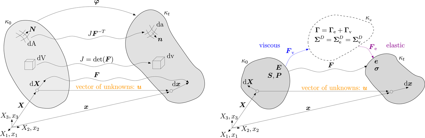
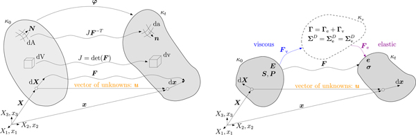
A distinction between different configurations is necessary to consider finite deformations. The reference configuration κ 0 is defined by all positions X of material points in an initially undeformed body. The current configuration κ t is specified by a unique deformation mapping φ that relates the position X of material points to positions x of spatial points depending on the external load until time t. Through the displacement field u = x − X the particle position X in the reference configuration is related to its position x in the current configuration (Fig. 2, left). The differential equations for finite viscoelasticity can be formulated with respect to the reference or the current configuration. Here we focus on a formulation with respect to the reference configuration, which is frequently applied in solid mechanics.
For the finite viscoelastic Maxwell material model, it is necessary to distinguish between reference (κ 0), current (κ t) and intermediate (κ v) configurations. In the intermediate configuration (dashed line in the right panel) the viscoelastic material equations are derived.
The deformation gradient F characterizes the material gradient of motion
 $${\bi F}({\bi X},t) = {\displaystyle{\partial {\bi x}} \over {\partial {\bi X}}} = {\displaystyle{\partial {\bi u}} \over {\partial {\bi X}}} + {\bi I}. $$
However, the deformation gradient F also includes rigid body motions composed of translations and rigid body rotations. These motions preserve the distance between two points of a continuum and induce no strains. Thus the Green-Lagrange strain tensor
 $$ {\bi E} = {\displaystyle{ 1 \over 2}} \left({\bi C}- {\bi I} \right) $$
is defined as a reasonable strain measure in the reference configuration with the right Cauchy-Green tensor given by
 $$ {\bi C} = {\bi F}^T {\bi F}. $$
Accordingly, the strain measure in the current configuration is the Euler-Almansi strain tensor
 $$ {\bi e} = {\displaystyle{1 \over 2}} \left({\bi I} - {\bi b}^{-1} \right) $$
with the left Cauchy-Green tensor defined by
 $$ {\bi b} = {\bi FF}^T. $$
For rigid body motions, the deformation gradient F does not vanish, and hence, it is not a suitable strain measure. In contrast, the Green-Lagrange E and the Euler-Almansi e strain tensors are zero for rigid body motions (translation and rotation). Note that the infinitesimal strain tensor ε is also not applicable, as it is non-zero for finite rigid body rotations.
The quasi-static momentum balance in the reference configuration is given by
 $$ {\rm Div} \;{\bi P} + {\bi f}_0 = {\bf 0} $$
where Div ( · ) is the divergence with respect to the reference configuration. The equation for the volume force f0 = −(J ρ iceg)ez contains the Jacobian determinant  $J = \det ({\bi F})$ due to the transformation rule for volume elements dv = J dV (Fig. 2, left). The first Piola-Kirchhoff stress tensor P = J σF−T includes the transposed inverse of the deformation gradient F−T = (F−1)T. The relation between P and the Cauchy stress tensor σ is obtained based on the vector of stress resultant force df = σn da = PN dA and Nanson's formula J F−TN dA = n da. Nanson's formula provides the relation of infinitesimal area elements in the current and the reference configuration (Fig. 2, left) with the unit normal vectors n (current configuration) and N (reference configuration).
The formulation for finite viscoelasticity uses the conceptual multiplicative decomposition of the deformation gradient F (Lee, Reference Lee1969; Simo and Hughes, Reference Simo and Hughes2000) into rate-independent (elastic) and rate-dependent (viscous) parts
 $$ {\bi F} = {\bi F}_{\rm e} {\bi F}_{\rm v} $$
to represent the material behavior (Fig. 2, right). Since the strain cannot be additively decomposed in a purely elastic and purely viscous part either in the reference or in the current configuration, the intermediate configuration κ v is considered. All essential equations are formulated in the intermediate configuration κ v. As a motivation the additive decomposition of the strain tensor Γ in the intermediate configuration reads
 $$\eqalign{ {\bf \Gamma } &= {\bi F}_{\rm v}^{-T} {\bi EF}_{\rm v}^{-1} = \displaystyle{1 \over 2}{\bi F}_{\rm v}^{-T} ({\bi F}^T{\bi F}-{\bi I}){\bi F}_{\rm v}^{-1} \cr & = \displaystyle{1 \over 2}\left( {{\bi F}_{\rm e}^T {\bi F}_{\rm e}-{\bi F}_{\rm v}^{-T} {\bi F}_{\rm v}^{-1} } \right) = {\bf \Gamma }_{\rm e} + {\bf \Gamma }_{\rm v}} $$
(cf. the small deformation model). The elastic and viscous strain tensor are given by  ${\bf \Gamma}_{\rm e}= 1/2 ({\bi F}_{\rm e}^T {\bi F}_{\rm e} - {\bi I})$ and ${\bf \Gamma}_{\rm v} = 1/2 ({\bi I} - {\bi F}_{\rm v}^{-T} {\bi F}_{\rm v}^{-1})$, respectively. Note that ${\bi F}_{\rm v}^{-T} (\cdot) {\bi F}_{\rm v}^{-1} $ describes the push-forward operation of strain tensors from the reference to the intermediate configuration.
In a viscoelastic material the stress tensor Σ of the intermediate configuration is assumed to depend on the rate-independent part of the deformation gradient
 $$ {\bf \Sigma} = f\,({\bi F}_{\rm e}). $$
A generalization of Hooke's law is given by
 $$ {\bf \Sigma} = {\opf {E}}\;{\bf \Gamma}_{\rm e}$$
with the constant forth order elasticity tensor  ${\opf E}$. For an isotropic material this relation simplifies to
 $$ {\bf \Sigma} = \lambda {\rm tr} \left ({\bf \Gamma}_{\rm e} \right) {\bi I} + 2 \mu {\bf \Gamma}_{\rm e}. $$
This constitutive equation is also addressed as Saint Venant-Kirchhoff material. Based on the additive decomposition of the strain tensor, Eqn. (18) can be expressed by the viscous strain tensor  ${\bf \Gamma}_{\rm v}$ via
 $$ { \bf \Sigma} = \lambda {\rm tr} \left({\bf \Gamma} -{\bf \Gamma}_{\rm v} \right) {\bi I} + 2 \mu ({\bf \Gamma} -{\bf \Gamma}_{\rm v}). $$
Analogous to the small strain formulation, an incompressible viscous flow is assumed which leads to a trace-free viscous strain rate. In particular, suitable initial conditions lead to  ${\rm tr} \left({\bf \Gamma}_{\rm v} \right) = 0 $ (Christmann, Reference Christmann2017). Hence, Eqn. (19) results in
 $$\eqalign{& {\bf\Sigma} = \underbrace{{\left( {\lambda + \displaystyle{2 \over 3}\mu } \right)}}_{{ = K}}{\rm tr}\left( {\bf \Gamma } \right){\bi I} + 2\mu \left[ {{\bf \Gamma }-{\bf \Gamma }_{\rm v}-\displaystyle{1 \over 3}{\rm tr}\left( {{\bf \Gamma }{\rm - }{\bf \Gamma }_{\rm v}} \right){\bi I}} \right] \cr & \quad = \underbrace{{\left( {\lambda + \displaystyle{2 \over 3}\mu } \right){\rm tr}\left( {\bf \Gamma } \right){\bi I}}}_{{ = {\bf\Sigma} ^{\rm vol}}} + \underbrace{{2\mu \left[ {{\bf \Gamma }_{\rm e}-{1\over 3}{\rm tr}\left( {{\bf \Gamma }_{\rm e}} \right){\bi I}} \right]}}_{{ = {\bf\Sigma} ^D}}} $$
The structure of Eqn. (20) resembles the stress/strain relation of the small deformation model (Eqns. 3, 4). The decomposition of the stress tensor into a volumetric Σvol and deviatoric part ΣD is recovered. The volumetric part of the stress tensor is expressed by the trace of the strain tensor. This trace is related to the relative change in volume ΔV/V in the case of small strains. Consequently, this ansatz is valid for finite deformations but moderate (small) strains.
Another possible finite deformation formulation is known as the neo-Hookean formulation. The investigation of calving at ice shelves using neo-Hookean material leads to identical results as the Saint Venant-Kirchhoff material (Christmann, Reference Christmann2017). Hence, the Saint Venant-Kirchhoff material model is used in the following.
In order to derive the evolution equation of the internal variable  ${\bi C}_{\rm v} = {\bi F}_{\rm v}^T {\bi F}_{\rm v} $, the strain-rate tensor of the intermediate configuration is needed. The push-forward operation of the rate of the Green-Lagrange strain tensor $\dot {\bi E}$ to the intermediate configuration renders the objective lower Oldroyd rate ${ \bf \mathop \Gamma \limits^\Delta}$ as a Lie time derivative
 $$ {\mathop {\bf \Gamma} \limits^\Delta} = {\bi F}_{\rm v}^{-T} {\dot {\bi E}} {\bi F}_{\rm v}^{-1} = {\bi F}_{\rm v}^{-T} \left(\dot {\overline {{\bi F}_{\rm v}^T {\bf \Gamma} {\bi F}_{\rm v}}} \right) {\bi F}_{\rm v}^{-1} = \dot{\bf \Gamma} + {\bi I}_{\rm v}^T {\bf \Gamma} + {\bf \Gamma} {\bi I}_{\rm v} $$
with the viscous deformation rate  ${\bi I}_{\rm v} = \dot {\bi F}_{\rm v} {\bi F}_{\rm v}^{-1}$. Lie time derivatives are always objective rates of a spatial tensor. However, the choice of an objective strain rate is not unique. In Haupt (Reference Haupt2000) the applicability of the Oldroyd rate to the Maxwell material model is shown, and in Christmann (Reference Christmann2017) investigations with the upper Oldroyd rate are discussed. Based on the additive decomposition of the total strain, the additive decomposition of the strain-rate tensor is also valid with the elastic ${\bf \mathop \Gamma \limits^\Delta}_{\rm e} = {\dot {\bf \Gamma}}_{\rm e} + {\bi I}_{\rm v}^T {\bf \Gamma}_{\rm e} + {\bf \Gamma }_{\rm e} {\bi I}_{\rm v}$ and the viscous strain rate ${\bf \mathop \Gamma \limits^\Delta}_{\rm {v}} = \dot {\bf \Gamma}_{\rm v} + {\bi I}_{\rm v}^T {\bf \Gamma}_{\rm v} + {\bf \Gamma}_{\rm v} {\bi I}_{\rm v}}$. To derive the flow relation in the intermediate configuration, the deviatoric elasticity relation is assumed to be proportional to the viscous strain rate ${\bf \mathop \Gamma \limits^\Delta}_{\rm v}$ (cf. Eqn. 4)
 $$ 2 \eta {\mathop {\bf \Gamma} \limits^\Delta}_{\rm v} = 2 \mu \left[{\bf \Gamma} -{\bf \Gamma}_{\rm v} - {\displaystyle{1 \over 3}}{\rm tr} \left({\bf \Gamma} -{\bf \Gamma}_{\rm v} \right) {\bi I} \right] = 2 \mu {\bf \Gamma}_{\rm e}^D. $$
Note that  ${\rm tr} \left ({\bimathop \Gamma \limits^\Delta}_{\rm v} \right)$ vanishes. To transform Eqns. (20) and (22) back to the reference configuration, where the quasi-static momentum balance is solved, the pull-back operation ${\bi F}_{\rm v}^{-1} (\cdot) {\bi F}_{\rm v}^{-T}$ for contravariant second order tensors is used. The second Piola-Kirchhoff stress tensor S in the reference configuration becomes
 $$\eqalign{ {\bi S}& = {\bi F}_{\rm v}^{-1} {\vector \bf \Sigma }{\bi F}_{\rm v}^{-T} = \displaystyle{{\lambda + (2/3)\mu } \over 2}\left[ {{\rm tr}\left( {{\bi CC}_{\rm v}^{-1} } \right)-3} \right]{\bi C}_{\rm v}^{-1} \cr & \quad + \mu \left[ {{\bi C}_{\rm v}^{-1} {\bi CC}_{\rm v}^{-1} -\displaystyle{1 \over 3}{\rm tr}\left( {{\bi CC}_{\rm v}^{-1} } \right){\bi C}_{\rm v}^{-1} } \right].} $$
This is the elasticity relation in the reference configuration. In order to solve the quasi-static momentum balance (Eqn. 13) in the reference configuration, the first Piola-Kirchhoff stress tensor is given by P = FS. The pull-back operation  ${\bi F}_{\rm v}^T (\cdot ) {\bi F}_{\rm v}$ for covariant second order tensors such as the viscous strain rate of Eqn. (22) provides the evolution equation for the internal variable ${\bi C}_{\rm v}$
 $$ \eta \dot{\bi C}_{\rm v} = \mu \left({\bi C} - \displaystyle{1 \over 3} {\rm tr} \left({\bi C} {\bi C}_{\rm v}^{-1} \right) {\bi C}_{\rm v} \right). $$
A summary of the system of differential equations to be solved to get the displacement vector u is given in Table 1.
Summary of solved equations and unknowns for the finite viscoelastic Maxwell model

3.2.1. Glen's flow law
So far a constant viscosity η has been used. In the following, a non-constant viscosity based on Glen's flow law will extend the linear rheology. To this end a rate-dependent dashpot is introduced in the rheological model (Fig. 1). To be consistent with the large deformation formulation, the nonlinear viscosity is introduced in the intermediate configuration as an additional constitutive assumption. Glen's flow law states
 $$\eta = \displaystyle{1 \over {2A \sigma_{{\rm eff}}^{n-1} }},\quad \sigma _{{\rm eff}} = {\rm }\sqrt {\displaystyle{1 \over 2}{\rm tr}{\left( {{\bisigma }^D} \right)}^2} $$
with the rate factor A, the stress exponent n=3, and the effective stress σ eff (Greve and Blatter, Reference Greve and Blatter2009). For the viscoelastic Maxwell material model, the viscosity η appears only in the flow relation (Eqn. 22). The nonlinear viscosity for the finite deformation model is expressed by
 $$ 2 \eta {\bf \mathop \Gamma \limits^\Delta}_{\rm v} = 2 \, {\displaystyle{1} \over {2 A \, \Sigma_{\rm eff}^{n-1}}} \, {\bf \mathop \Gamma \limits^\Delta}_{\rm v} = 2 \, {\displaystyle{1} \over {2 A \, \Sigma_{\rm eff}^{2}}} \, {\bf \mathop \Gamma \limits^\Delta}_{\rm v}, \quad \Sigma_{\rm eff} = \sqrt{{\displaystyle{1} \over {2}} {\rm tr} \left({\bf \Sigma}^{D} \right)^2} $$
with the effective stress Σeff computed in the intermediate configuration. The pull-back operation to the reference configuration yields
 $$\eqalign{ {\bi F}_{\rm v}^T 2\eta {\mathop {\bf \Gamma }\limits^{\Delta}}_{\rm v}{\bi F}_{\rm v} &= \displaystyle{1 \over {A \Sigma _{{\rm eff}}^2 }}{\bi F}_{\rm v}^T {\mathop {\bf \Gamma }\limits^\Delta} _{\rm v}{\bi F}_{\rm v} = {\displaystyle{1 \over {A \Sigma _{{\rm eff}}^2 }} \displaystyle{1 \over 2}{\mathop {\bi C}\limits^{\bi .}}_{\rm v}} \cr & = \underbrace{{\displaystyle{1 \over {A {\rm tr}{\left( {{\bf \Sigma }^D} \right)}^2}}}}_{{ = \eta _{{\rm Glen}}}}\mathop {{\bi C}_{\rm v}}\limits^{.}} $$
where η Glen denotes the nonlinear Glen-type viscosity. The deviatoric stress tensor ΣD is given by (cf. Eqn. 20)
 $$ {\bf \Sigma}^{D} = 2 \mu \left[{\bf \Gamma}_{\rm e} - {\displaystyle{1 \over 3}} {\rm tr} \left({\bf \Gamma}_{\rm e} \right) {\bi I} \right] $$
and thus the effective stress in the intermediate configuration reads
 $$ 2\, \Sigma_{\rm eff}^2 = {\rm tr} \left({\bf \Sigma}^{D} \right)^2 = 4 \mu^2 \left[{\rm tr} \left({\bf \Gamma}_{\rm e}^2 \right) - {\displaystyle{1 \over 3}} \left({\rm tr} \left({\bf \Gamma}_{\rm e} \right) \right)^2 \right]. $$
The elastic strain tensor  ${\bf \Gamma} _{\rm e} $ can be expressed by quantities of the reference configuration (cf. Eqn. 23)
 $$ {\rm tr} \left({\bf \Gamma}_{\rm e} \right) = {\displaystyle{1} \over {2}} \left[{\rm tr} \left({\bi CC}_{\rm v}^{-1} \right) -3 \right] \quad {\rm with} \quad {\bf \Gamma}_{\rm e} = {\displaystyle{1} \over {2}} \left[{\bi CC}_{\rm v}^{-1}- {\bi I} \right]. $$
In the end, the effective stress of Eqn. (29) results in
 $$ 2 \Sigma _{{\rm eff}}^2 = \mu ^2 {\rm tr}{\left( {{\bi CC}_{\rm v}^{{\rm - 1}} } \right)}^2-{1\over 3}\mu^2 \left({\rm tr} {({\bi CC}_{\rm v}^{{\rm - 1}} }) \right)^2 $$
with
 $$ {\rm tr} \left( {{\bf \Gamma }_{\rm e}^{\rm 2} } \right) ={1\over 4}\left[ {\rm tr} \left( {{\bi CC}_{\rm v}^{{\rm - 1}} } \right)^2 -2{\rm tr} \left( {{\bi CC}_{\rm v}^{{\rm - 1}} } \right)+3 \right] $$
and
 $$ \big({\rm tr} \left( {{\bf \Gamma }_{\rm e} } \right)\big)^2={1\over 4}\left[ \big({\rm tr} ( {{\bi CC}_{\rm v}^{{\rm - 1}} } )\big)^2 -6{\rm tr} \left( {{\bi CC}_{\rm v}^{{\rm - 1}} } \right)+9 \right].$$
Hence, it is possible to compute the nonlinear viscosity
 $$ \eta_{\rm Glen}= {\displaystyle{1} \over {A \,2 \Sigma_{\rm eff}^{2}}} = {\displaystyle{1} \over {A \, {\rm tr} \left({\bf \Sigma}^{D} \right)^2}} $$
solely by quantities of the reference configuration.
4. MODELING CONCEPT
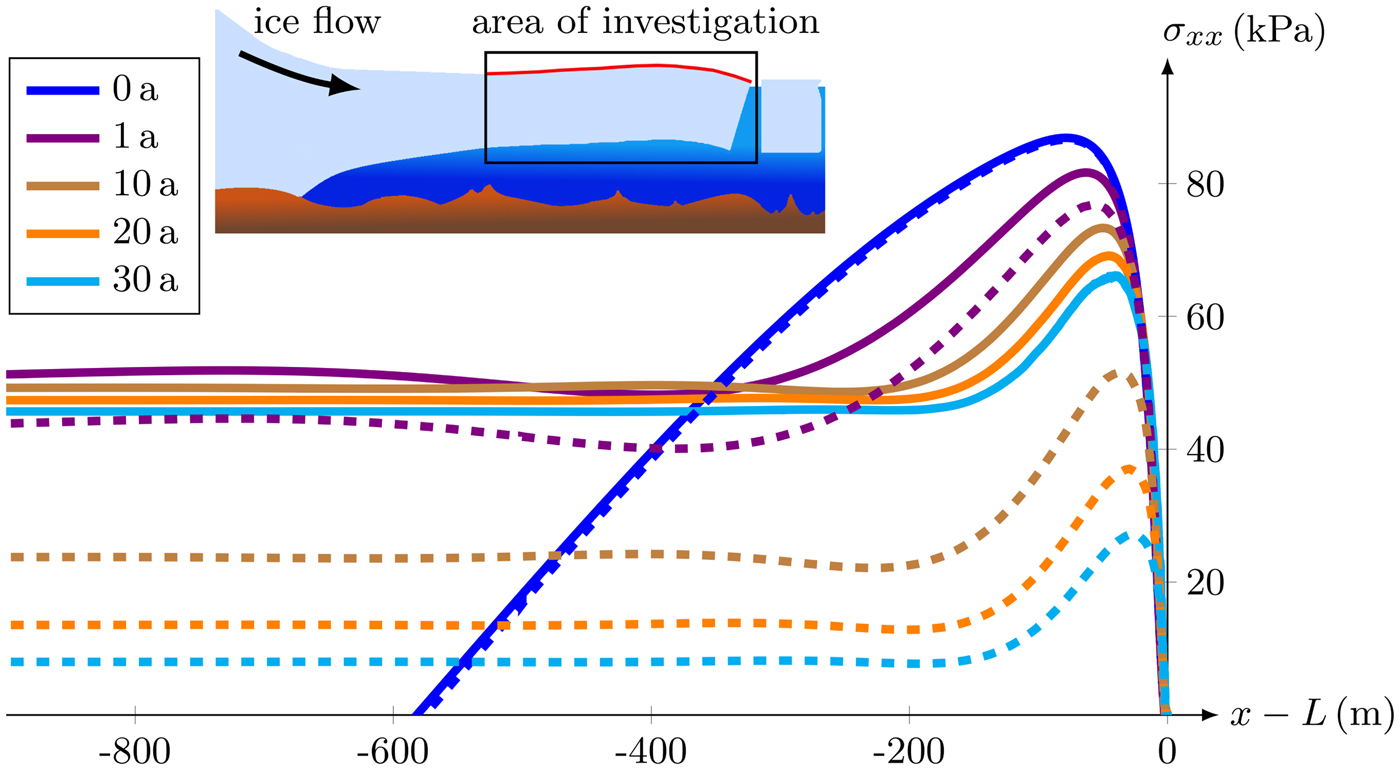
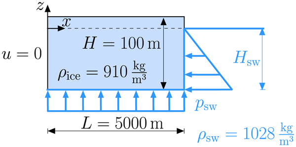
In this study the focus is on a geometry that resembles the Ekström Ice Shelf, East Antarctica. This specific ice shelf is an example where small-scale calving occurs despite a crevasse-free surface. Ground-penetrating radar has been used to determine the ice thickness along streamlines (Lohse, Reference Lohse2012). The thinning in flow direction up to the calving front is ~111 m over a distance of 12 km. In Fig. 3, the stress component σxx in flow direction is depicted for this measured ice shelf geometry. The transition from the small region of tension (green) to compression (pink) is highlighted by the black line, while each contour of the stress component indicates a difference of 100 kPa in gray. In order to describe small-scale calving, the maximum values of stress and strain are important and occur near the termination (cf. the stress distribution in Fig. 3). In this relevant area near the ice front it is sufficient to consider a model geometry with a constant thickness (Christmann, Reference Christmann2017), as only negligible thickness gradients appear. In the present work, the initial ice shelf domain has a length of L = 5000 m and a thickness of H = 100 m (Fig. 4). The ice flows from the left to the right and calving processes happen at the right end (ice front). Common material values are assumed to model polycrystalline ice with the elastic constants represented by Young's modulus E = 9 GPa (Gammon and others, Reference Gammon, Kiefte, Clouter and Denner1983; Rist and others, Reference Rist, Sammonds, Oerter and Doake2002), Poisson's ratio ν = 0.325 (Schulson and Duval, Reference Schulson and Duval2009), and the constant viscosity η = 1014 Pa s (Greve and Blatter, Reference Greve and Blatter2009).
Stress component σ xx in a cross section of the Ekstroem Ice Shelf. Black line highlights the transition from tension (green) into compression (pink), and gray lines are the contours at each 100 kPa of the stress component.

The idealized ice shelf domain and its boundary conditions representing the forces acting on an ice shelf.

In addition, the corresponding boundary conditions are shown in Fig. 4. The area of investigation for small-scale calving is far away from the grounding line where the ice begins to float. Consequently, a constant inflow velocity is present across the whole ice thickness since the missing traction of the ground causes a plug flow inside the ice shelf (Greve and Blatter, Reference Greve and Blatter2009). At the inflow, this characteristic is described by a constant displacement, i.e. a Dirichlet boundary condition. Prescribed displacement values entail rigid body motions, by which the examined stress and strain states are unaffected. Hence, the normal displacement at the inflow boundary is set to zero. For H = 100 m, the boundary condition at the inflow does not affect the stress and strain evolution near the ice front if the length L is larger than 3000 m (Christmann, Reference Christmann2017).
The traction t at all other boundaries reads
 $$ {\bi t} = {\bisigma} {\bi n} = p {\bi n}, $$
where p is the water pressure that acts in the normal direction. At the bottom, the water pressure must balance the weight of the ice to ensure buoyancy equilibrium. The thickness of ice below the sea level results in a draft H sw = ρ ice/ρ sw H with the sea water density ρ sw = 1028 kg m−3 and the ice density ρ ice = 910 kg m−3. At the bottom and the ice front, the water pressure is given by
 $$p = \left\{ {\matrix{{\rho_{\islant-20% {sw}}g(-z-w)} \hfill & {{\rm for}\,\;z + w \le 0} \hfill \cr 0 \hfill & {{\rm else}} \hfill \cr} } \right.$$
and increases with the water depth. In the above equation, g = 9.81 m s−2 is the gravity acceleration and w the displacement in z-direction influenced by the bending moment of the water pressure at the ice front. The second line of Eqn. (36) guarantees that if the surface extents above sea level (freeboard), this part is traction-free. This traction-free condition is also applied on the top surface.
For the finite deformation model, the differential equation system is formulated in the reference configuration. The Dirichlet condition at the inflow does not change, and the corresponding traction boundary condition in the reference configuration is given by
 $$ {\bi t}_0 = {\bi P} {\bi N} = P_0 {\bi N} = p J {\bi F}^{-T} {\bi N} $$
with the pressure P 0 in the reference configuration. This equation results from Nanson's formula JF −TN dA = n da describing the relation of boundary conditions in the reference and the current configuration. Hence, the traction is not only dependent on the displacement w of the boundary but also on the actual variation of the ice shelf geometry represented by the deformation gradient F.
In viscous ice-sheet models, a nonlinear rate-dependent viscosity is used. To include this by a nonlinear dashpot in the viscoelastic Maxwell model, it is necessary to replace the constant viscosity by a power law dependent on the effective stress (Eqn. 34). This nonlinear Glen-type viscosity is pulled to the reference configuration in which the system of differential equations is solved. Thus, the equation of the Glen-type viscosity is modified by C and the internal variable  ${{ \bi {C}}_{\rm v}}$. In the end, the Glen-type viscosity as well as the quasi-static momentum balance (Eqn. 13) depends on the deformation gradient F.
5. NUMERICS
The mathematical models have been implemented into the commercial finite element software COMSOL.Footnote 1 Previous studies have demonstrated that the influence of the lateral boundaries vanishes in ice shelves with a width of a few kilometers (Christmann, Reference Christmann2017). The area affected by the lateral boundaries depends on the thickness. In the case of H = 100 m, a width smaller than 7 km influences the stress and strain states in the center. For wider ice shelves, the state of plane strain is reached as the processes in the middle are no longer influenced by the constraints at lateral boundaries. In this situation it is sufficient to describe the process of calving as a two-dimensional problem in the x−z-plane assuming plane strain conditions in y-direction.
For the small deformation model COMSOL determines the discrete nodal displacements u and the nodal viscous strain tensor  ${{ \bi { \varepsilon }}_{\rm v}}$ in every time step. The stress and strain states can be computed from the displacements and the viscous strain tensor in a postprocessing step. The time steps are auto-controlled by the (time-dependent) solver of COMSOL. The discretization consists of triangular elements with quadratic Lagrange shape functions of second order polynomials. The maximum element size is 50 m. At the ice front and the ice shelf surface, the mesh is refined to an element length of 2 m within the first 1000 m upstream from the ice front. This mesh results in 147 254 degrees of freedom. A coarsening of the mesh (maximum element length of 5 m for the first kilometer away from the front) leads to a 2% difference of the maximum stress value at the upper surface.
In the finite deformation model the system of differential equations is solved in three-dimensional space as the reduction to two dimensions is not straightforward. The three-dimensional formulation allows for a direct implementation of the constitutive relations (Eqns. 8, 10, 23) without any further considerations. However, the displacement v in the y-direction is fixed for the lateral surfaces by appropriate boundary conditions enforcing plane strain conditions. The balance of linear momentum (Eqn. 13) and the evolution equation (Eqn. 24) are solved in the reference configuration to obtain the unknown nodal displacement vector u and the internal variable tensor  ${{ \bi {C}}_{\rm v}}$ (Table 1). The domain is discretized using triangular prisms with a unit width in y-direction. This is sufficient due to the plane strain assumption. Quadratic Lagrange shape functions are used in the triangles on the lateral surfaces. The maximum edge length of the triangles is equal to the maximum element length for the small deformation model and results in 506 574 degrees of freedom. The increase in the degrees of freedom is caused by the fact that the finite deformation model has twice as many nodes (three vs. two dimensional) and nearly twice as many unknowns (9 vs. 5) compared with the small deformation model. Consequently, the number of the degrees of freedom is roughly four times higher in the finite deformation model.
The independence of the results from the discretization and the length L has been verified for both model approaches. Based on the nonlinearity of the material formulation in the finite deformation model, the choice of the resolution for the spatial discretization becomes crucial. The results are strongly influenced by the regions where boundary conditions change, for instance by the transition at the sea level where the traction free condition of the freeboard is changing into the depth-dependent water pressure. If the spatial discretization is too coarse, the boundary condition cannot be resolved accurately enough. Artificial oscillations occur in stress and strain states at those regions of the freeboard that are crucial to determine small-scale calving (Christmann, Reference Christmann2017). Thus, for the finite element simulations of the two viscoelastic models used here a high spatial resolution is required.
6. RESULTS
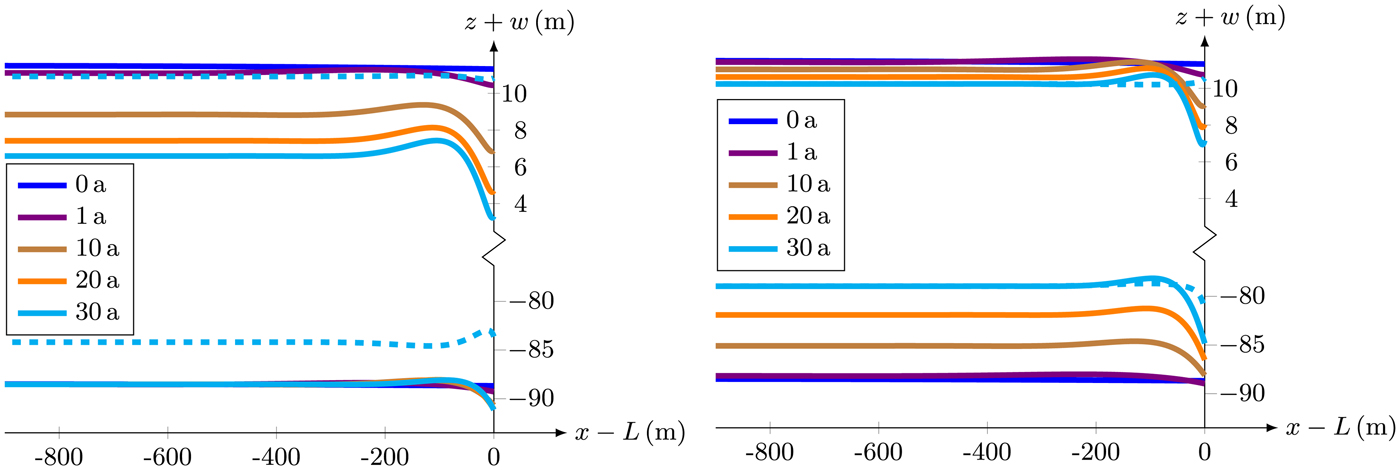
In order to show differences between the results of the small and finite deformation model, the evolution of the geometry based on deformations is analyzed with time. Resulting positions of top and bottom surfaces are displayed in Fig. 5 for different points in time. In the left panel, the temporal evolution of the geometry obtained with the small deformation model is depicted. The position of the ice draft remains constant, with a draft of H sw = 88.5 m, while the upper surface (and thus also the freeboard) decreases monotonously with time. The geometry at t = 30 a assuming buoyancy equilibrium is additionally given by the dashed line. Using the small deformation model, the buoyancy equilibrium is clearly not fulfilled as the dashed and solid cyan lines do not coincide. In contrast, ice surface and base match for the finite deformation model with the buoyancy equilibrium (exemplarily shown for t = 30 a in Fig. 5, right panel) due to the fact that both surfaces evolve over time. Only near the calving front (− 200 m ≤ x − L ≤ 0 m), the disturbance of the boundary condition of the ice front (eccentric water pressure) leads to deviation from the buoyancy equilibrium.
Temporal evolution of the positions of the top and bottom surfaces attained by the small (left) and finite deformation (right) models. Dashed lines show the positions of the buoyancy equilibrium at time t = 30 a.
Tensile stresses only occur for σ xx (Fig. 3) as the stress σ zz in vertical direction depicts the hydrostatic pressure. The maximum tensile stress in the ice shelf is obtained at the top surface in flow direction (not shown here; cf. Christmann and others, Reference Christmann, Rückamp, Müller and Humbert2016b). This maximum is located close to the calving front (Fig. 6) and is caused by the bending moment of the depth-dependent water pressure at the ice front. As thicker the ice front, the higher is the stress at the surface for a purely elastic material model (Christmann, Reference Christmann2017). For a purely viscous material the stress distribution decreases in time as the ice shelf expands in flow direction and the ice thickness decreases (Christmann and others, Reference Christmann, Plate, Müller and Humbert2016a). In the viscoelastic Maxwell model, the elastic stress distribution is achieved directly at t = 0 a and after a first increase (shown later on for the stress maximum in Fig. 8), the tensile stress at the top surface reduces in time.
Stress component σ xx at the top surface using the concept of finite deformation (solid lines) vs. the assumption of small deformations (dashed lines). Area of investigation is additionally shown in a cross section of an ice sheet – ice shelf model that is deformed based on the boundary conditions (exaggerated deformation).
Initially the stress responses are identical for finite and small deformation models (blue curves in Fig. 6). Over time, the small deformation model (dashed lines) leads to a faster decrease of the maximum stress than the finite deformation model (solid lines). Crucial differences occur at the latest when t = 10 a (brown curves in Fig. 6). At this point in time, the maximum stress values differ by about 30%. However, differences are already identifiable at t = 1 a when the maximum of the dashed purple curve is 6%, namely 4.8 kPa, lower than the maximum of the solid purple curve.
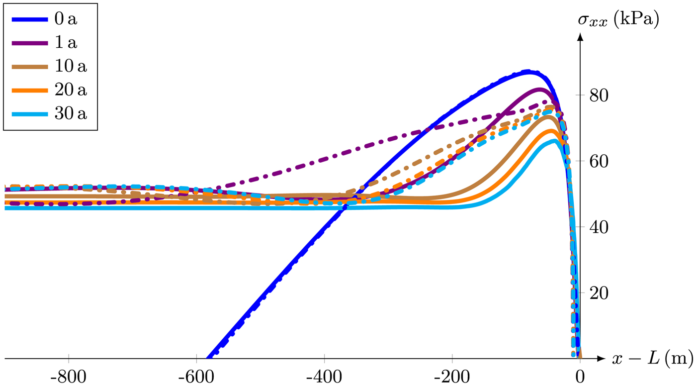
Thus far, all results are obtained using a constant viscosity η = 1014 Pa s. For the finite deformation model, the stress evolution at the top surface using this constant viscosity is compared with stress results using a nonlinear Glen-type viscosity (dash-dotted lines in Fig. 7). The viscosity must not have any influence at t = 0 a in the viscoelastic Maxwell case and therefore the constant rate factor A = 10−25 s−1 Pa−3 is chosen. We do not include any temperature dependence. As expected, the viscosity does not have any influence at t = 0 a. The maximum stress value at t = 1 a is 4% lower for nonlinear viscosity, while this reverses at t = 4 a. For t = 30 a, the maximum stress applying a constant viscosity is 12% lower than for a nonlinear viscosity.
Stress component σ xx at the top surface for the finite deformation model using a constant viscosity η = 1014 Pa s (solid lines) compared with the results obtained with a nonlinear Glen-type viscosity (dash-dotted lines).
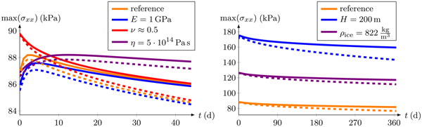
The impact of other material and geometrical parameters on the maximum stress is presented in Fig. 8. For these studies, a constant viscosity is assumed to separate the effects. A decrease of Young's modulus makes the material softer. A reduction of Young's modulus from E = 9 GPa (reference) to E = 1 GPa (Vaughan, Reference Vaughan1995) results in a small decrease of the maximum tensile stress (Fig. 8, left). The influence of an incompressible Poisson's ratio ν ≈ 0.5 is slightly larger, but the initial stress increase is missing for finite (solid lines) and small (dashed lines) deformation models. Furthermore, the effect of both elastic parameters becomes negligible for t > 45 d. Differences of ~2 kPa appear in the stress for both model formulations at t = 45 d (Fig. 8, left). The difference between those stress results increases nonlinearly. The constant viscosity is also varied to demonstrate that the effect of a larger value is equivalent to increasing the time until the highest stress value is reached. However, this does only affect timing, not the achieved stress values.
Evolution of maximum stress at the top surface with time, dependent on different material (left) and geometric parameters (right) using the finite (solid lines) and small (dashed lines) deformation models.

In addition, the effect of a modified geometry is investigated. The thickness of the ice shelf almost linearly controls the computed stress state and hence the maximum stress value (blue and orange curves in Fig. 8, right). The last parameter considered is the ice density. Using GPS and ground-penetrating radar measurements at the Ekström Ice Shelf, a mean density of ρ ice = 822 kg m−3 was determined. The decrease of the ice density ρ ice = 910 kg m−3 for pure ice to the mean value ρ ice = 822 kg m−3 (purple lines) results in an increase of the freeboard thickness due to the buoyancy equilibrium. In consequence, the stress values increase at the upper surface.
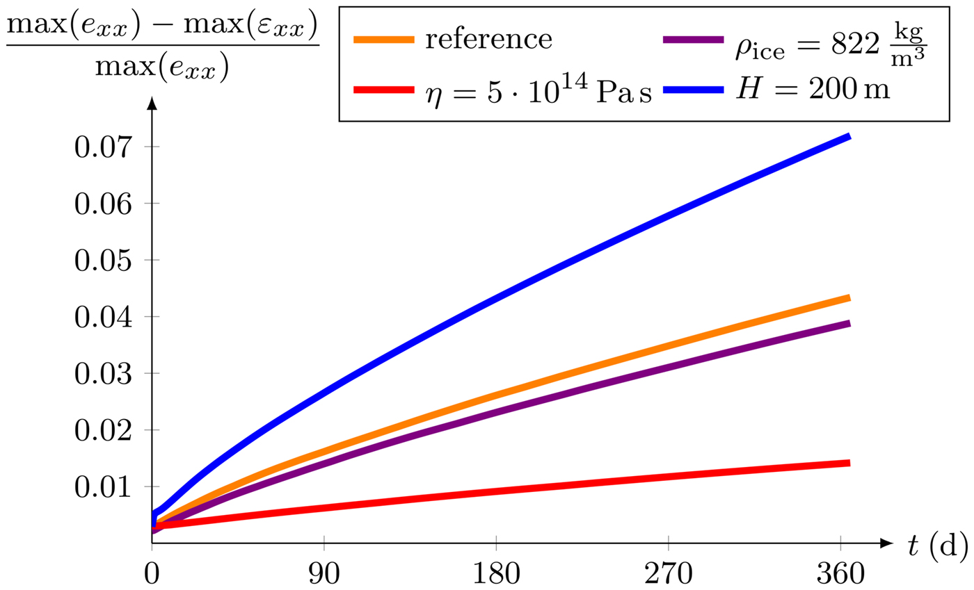
At last, the strain in flow direction is investigated as it is the largest strain component. In particular, its maximum is located at the upper surface (Christmann, Reference Christmann2017). For the finite deformation model, the Euler-Almansi strain e xx is analyzed as this is a possible strain measure in the current configuration. In this parameter study, only the relative strain difference between the strain obtained by the finite and the small deformation models is discussed in more detail (Fig. 9). Using the finite deformation approach, the strain is always higher than the strain computed with the small deformation model. The relative difference of both model formulations increases nonlinearly. An increase in viscosity by a certain factor results in strain growth divided by this factor, and hence smaller strain states are reached. All other elastic material parameters have almost no influence on the strain distribution in a time interval of one year. Therefore, these strain results are not explicitly included in Fig. 9 but are similar to the orange curve. A lower ice density slightly decreases the relative difference of the strain values obtained by the two model approaches in contrast to a thicker ice shelf in which this relative difference is higher: doubling the ice thickness leads to almost half the time to reach similar strain values with the small deformation model. The maximum strain values increase linearly with time and are given at t = 1 a in Table 2 for both models.
Relative difference between the maxima of the strain components e xx and ε xx computed with the finite and small deformation model, respectively.
Maximum strain values in flow direction obtained after 1 year. The strain in the small as well as the finite deformation model increases linearly with time

7. DISCUSSION
In Antarctica, small-scale calving occurs on intervals of several weeks to few years. During this period of time, the spreading in the flow direction leads to the largest deformation and elongates the ice shelf up to a few hundreds of meters. The goal of this work is not to establish a unique calving rate but to assess which material formulation is suitable for establishing calving laws. The results of the small deformation model shown above coincide with the ones of the more sophisticated finite deformation model for short time periods only. As long as the strain values remain small, a linearized strain tensor can be assumed. This restriction gives rise to the necessity of using a finite deformation model if one studies several consecutive calving events or flow of hundreds of meters between those events. In order to analyze the time period in which the small deformation model is adequate, the main differences resulting from these two formulations are discussed subsequently.
In consequence of the viscous stretching of the ice shelf, it thins out with time. In the small deformation model, the bottom surface does not move. As there is no difference between the reference and actual configuration for the small deformation model, there is no way to adapt internal and external forces. The boundary condition at the bottom is at any time related to the initial situation and the weight of the ice is constant in time. This behavior induces the unphysical situation that the buoyancy equilibrium of the ice shelf is increasingly violated with progressing time (exemplarily shown in Fig. 5 for t = 30 a). The reason for this is that the current weight of the floating ice is not correctly balanced by the opposed buoyancy force. A small deformation model is presumably sufficient to simulate a single calving event, but the geometry must be readjusted after each event to satisfy the buoyant equilibrium. This procedure is undesirable as multiple subsequent calving events must be computed and a cumulative error of the evolving geometry must be prevented.
To solve this unwanted issue, a finite deformation formulation is established. For this modeling approach, the weight of the ice and the boundary conditions depend on the deformation gradient and are updated in each time step. Similar to simulations using a moving mesh (often applied in viscous laminar flow models), the internal and external forces are adapted to the evolved geometry. An undesired mesh degeneracy is avoided as all computations for the finite deformation model are done with the initial mesh in the reference configuration. Another advantage of solving the system of equations in the reference configuration is that the normal forces are not required in each time step. Only the normal vector of the reference configuration is needed to compute the boundary conditions.
At the beginning of the simulation, no deformations are present and the stress responses are identical for both model formulations (Fig. 6). The results for the reference parameters show that deformations of more than 5% (e.g. ε xx = 0.07 at t = 10 a) lead to differences of 30% for the maximum stress values and almost 20% for the maximum strain values. These differences for both model approaches are already significant at t = 2 a, where the stress differs by 10%, while the strain difference is 6.5%. The slower decrease of the maximum stress value for the finite deformation model has consequences for the stress-triggered calving criterion. However, the critical stress value σ crit = 330 kPa of Hayhurst (Reference Hayhurst1972) is not reached in any of the model approaches. A stress increase obtained for instance by a geometry variation can faster close the gap between the critical stress value and the prevailing maximum stress in the case of the finite deformation model. Hence, the stress state of the finite deformation model reaches more quickly a critical stress. The parameter that influences the maximum stress value most is the thickness. Obviously, the difference between the stresses of the two approaches increases faster for higher thicknesses (Fig. 8, right) as larger flow velocity leads to larger strain in shorter times. Thus, the assumption of linearized strain tensor is violated at an earlier point in time.
The stress distribution at the ice surface has the same bell-shaped form using Glen-type viscosity instead of a constant one. The nonlinear Glen-type viscosity is a function of the effective stress and thus of the deformation. The viscosity does not have any influence at the beginning of the simulation (Figs. 8, 9) as the instantaneous response is purely elastic in a viscoelastic Maxwell material. The stress response of the maximum tensile stress shows similar behavior as the one for the reference parameters. After a first slight stress increase, the maximum stress decreases in time. This stress decrease is faster for the nonlinear viscosity than for the constant one. The reason for that is the effective stress, which is large for large tensile stresses. Large effective stress results in small viscosity near the surface of the ice shelf (Eqn. 25) and hence in a fast stress decrease at the beginning of the simulation. The maximum stress value obtained by the nonlinear viscosity converges during the considered simulation time to a higher value of 75 kPa than the maximum stress value for the constant viscosity (Fig. 7). Considering a critical stress criterion for calving, the higher stress maximum will lead to higher calving rates for the Glen-type viscosity if the critical stress is reached based on, e.g., geometry variations. In the future, also differences to the formulation of a viscoelastic material model with a nonlinear viscosity inserted in the actual configuration (dependent on the effective Cauchy stress tensor) should be investigated. However, the assumption that these differences will be small is plausible as the elastic deformation gradient  ${{ \bi {F}}_{\rm e}}$, which is the connection between the intermediate and current configuration, is presumably small in our case.
In conclusion, if a stress criterion is used to describe calving events it is essential that the applied model represents the physical situation. All material and geometrical parameters that affect a faster strain increase involve an earlier need to use the finite deformation model. This is caused by the fact that external and internal forces (especially the boundary conditions) act on the current configuration and evolve in time. The most important point is that the small deformation model entails a different (smaller) calving rate. Consequently, it is essential to use a finite deformation model (preferably with a Glen-type viscosity) if several successive calving events are considered, or the calving event does not occur at an ice shelf in the first few years. In both cases, the current deformations in the flow direction are too large to fulfill the assumption of small deformations. The simplifying assumptions allowing to use a linearized strain tensor do not hold anymore. In the end, it is imperative not only for the understanding of calving processes to have a robust and useful material description that is based on physics.
After we found that a finite strain theory is here inevitable, we now want to understand the implications of stress and strain states on finding a calving law. There are three conceivable routes: (C1) criticality by critical stress, (C2) criticality by critical strain with strain after calving being initially the same as prior, and (C3) criticality by critical strain with reset of strain to zero. In order to define a calving law by the stress criterion (C1), other effects than the uncertainties in material or geometrical parameters must result in a sufficient stress increase. Continuous melting at the bottom surface of the ice shelf does not change the behavior of the maximum stress. Higher melt rates lead to a faster stress decrease as for the case of an overall constant thickness. Hence, the assumption of a constant thickness is reasonable to consider the influence of different parameters on quantities crucial for small-scale calving. The effect of the elastic parameters such as Young's modulus and Poisson's ratio fades away after 40 days, and only a higher viscosity has the impact to delay this influence. This fits closely the characteristics of a Maxwell material in which the characteristic time τ(η, E, ν) determines the temporal behavior but does not influence the achieved values. In the end, the viscosity plays an important role in determining the time between calving events. However, the maximum value and the position of calving is rather independent of the viscosity.
Another possibility to define a calving criterion is a critical strain value (C2). The ice shelf stretches in flow direction and the atmospheric pressure acts at the freeboard, where the strain has smaller resistance force than below the water surface. Consequently, the strain is highest at the upper surface. The strain distribution at this surface is comparable with the one of the stress (Christmann and others, Reference Christmann, Plate, Müller and Humbert2016a).
While the position of calving is independent of the critical strain, the timing depends on it. However, the value of critical strain is an unknown parameter that would have to be adjusted. In the end, a comparison with measurements of small-scale calving is absolutely essential to make meaningful statements on calving rates. Nevertheless, the evolving strain distribution can be examined independently of an exact critical value. After a calving event caused by an arbitrary critical strain value, the deformation initially decreases before it increases again. The critical value is reached faster and faster – caused by the strain history of the remaining ice shelf – leading to disintegration (Christmann, Reference Christmann2017). Only if the strain history is discarded after each calving event a critical strain criterion is conceivable (C3). With this procedure, constant calving rates are obtained. Here, the finite deformation model yields more critical situations than the small deformation model as the strain results are higher (Fig. 9). This effect is caused by the ice draft that declines in time meaning that the resulting stress at the ice front decreases over time for the finite deformation model. In contrast to the small deformation model in which the decrease of the top surface leads to a constant stress at the ice front boundary. The finite deformation model results in faster horizontal spreading of the ice shelf and hence in larger strain values.
In summary, criterion (C1) has the implication that calving rates depend on ice thickness leading to higher calving rates for thick ice shelves and may prohibit calving of very thin ice shelves. The criterion depends on a critical stress as a material property that may vary with porosity and thus firn properties, temperature and impurities. Hence it could be derived by laboratory tests or inversely from remote-sensing calving rates at appropriate locations. Criterion (C2) is as much justified from the physical basis as criterion (C1) but far less constrained. Criterion (C3) is as little constrained as criterion (C2); however, it leads to calving after a constant time period, while it remains difficult to justify strain to be removed in the ice shelf by just detaching an iceberg.
Thus, in order to establish a calving law for small-scale calving, one needs to assess how ice-sheet models could adopt this in future, in particular, as they rely only on viscous flow thus far. The question to be answered can be formulated as: does an ice-sheet model need to compute nonlinear viscoelastic material laws in order to be able to apply the criteria? Criterion (C1) could be used in large-scale ice sheet models, for example, in Earth system models as long as the time step is not significantly smaller than 1 year. For shorter time periods, one could consider computing a lookup table for stresses initiating calving. This table, which includes a correction term for the elastic contribution, must depend on different material parameters. Criteria (C2) and (C3) currently suffer from uncertainties in the critical strain, whereas criterion (C2) requires strain to be solved and is hence not applicable in viscous ice models. Criterion (C3) can potentially be applied to viscous models using a lookup table for the time schedule of calving that once again depends on different material parameters.
8. CONCLUSIONS
We presented a viscoelastic Maxwell model for small as well as finite deformations and its application to small-scale calving at ice shelves. At each point in time, the differences between the stress states in the two model formulations are higher than those for the strain. A difference of 5% between the strains in the material models for infinitesimal and finite strains is reached already after 1.25 a. After 10 a, the difference increases to 20%. This shows that for a study of several subsequent calving events or simulation times of more than 1 year, it is essential to apply a viscoelastic model using finite strain theory. This more sophisticated approach ensures consistency concerning the hydrostatic equilibrium, while the small deformation model (with linearized strain) produces a deviation from buoyancy equilibrium that grows larger with time. Furthermore, the consideration of a nonlinear viscosity leads to higher maximum stress values that converge to 75 kPa for a 100 m thick ice shelf. To include this formulation using finite strain theory in ice-sheet models requires a horizontal resolution of hundreds of meters in flow direction and only a few meters close to the calving front.
The evolution of stress and strain states obtained for typical geometries and material parameters suggests three different criteria for calving, which are all similarly justified but yield substantially different calving rates. While a stress criterion and a strain criterion without considering the strain history result in almost constant calving rates, a strain criterion considering the strain history forces the disintegration of the ice shelf. None of the criteria is yet constrained by critical thresholds for polycrystalline ice. However, regardless of maximum stress or strain criteria the finite deformation model leads faster to critical states and consequently to higher calving rates.
The finite strain formulation of the viscoelastic material model that we presented here for the application to calving may also be useful in other cases with short-term changes in loading and finite deformations. These may include the evolution of englacial and subglacial channels or tidal forcing of grounding line migration. An open question still remains whether it is necessary to include viscoelasticity in the whole domain or only in those parts where the short-term elastic response becomes essential and incorporating viscoelastic effects into current ice-sheet models is practical. In order to investigate small-scale calving at Antarctic ice shelves caused by the boundary perturbation at the ice front, it is sufficient to include the viscoelastic material model only within a few kilometers from the ice front. The processes further upstream are unimportant for small-scale calving at crevasse-free surfaces. It may be time for a new concept in ice-sheet modeling that tracks the strain history. Using this additional knowledge combined with a high-resolution mesh, a realistic representation of iceberg calving can eventually close one of the missing links between the ice sheet and ocean models.
ACKNOWLEDGMENTS
This work was supported by DFG priority program SPP 1158, project numbers HU 1570/5-1 and MU 1370/7-1. Parts of this work were also funded by the BMBF project GROCE (03F0778A). We thank the scientific editor Ralf Greve, two anonymous reviewers, and Olga Sergienko for careful reading and very helpful suggestions. We would also like to thank Vadym Aizinger and Ralph Timmermann for helpful comments and discussions.
APPENDIX
List of symbols


 Open access