

1. Introduction
This paper demonstrates how insurance companies can ensure the security, privacy, and confidentiality of their customer data while collaborating with other insurers. We propose utilising Federated Learning (FL) in insurance to allow secure collaboration on machine learning models. FL operates by bringing machine learning models to distributed data, fostering collaboration without direct data exchange. This paper presents a novel contribution: a tailored FL framework designed specifically for the insurance sector, complemented by a unique hyperparameter tuning approach. Access to the complete codebase is available via the following link: https://github.com/actuari/IFoA-FL-WP.git
Code documentation can be found in FL_usecase_docs.pdf in the docs folder of this repo. To motivate our use case, consider the scarcity that is often found in insurance data. For example, a life insurer trying to predict mortality rates of a small population such as the very elderly. There is often very little data on such a cohort e.g. those aged over 90 years old. Or a home insurer predicting the chance of a natural disaster such as a hurricane, or estimating capital requirements for a 1:200 year event. Or consider launching a new insurance product in a new market with no prior claims experience, or being exposed to a new emerging risk type.
Insurance data’s rarity and value provides insurers with some motivation to share it with each other to some extent. While pooling data can enhance model performance, it also exposes the data. Whilst insurers do often exchange obfuscated, limited, data for fraud and claims underwriting purposes, highly detailed, granular data is rarely shared.
Furthermore insurance data is often highly regulated and sensitive, which also prevents its exchange. Many markets impose stringent requirements such as the General Data Protection Regulation (GDPR) in the European Union. Insurance data can reveal a company’s strategy, pricing, inner workings, and other commercial secrets. It can also contain highly sensitive data on their customers such as their medical health history.
FL is a technique initially designed to build models such as text prediction on smartphones without requiring any smartphone data to leave the device and be seen by an external party. In this paper, the authors demonstrate how the same concept can be applied to insurance companies. Specifically, the authors use the freMTPL2freq car insurance dataset to mimic an entire insurance market’s claim experience. We then model this data set being split between 10 different independent insurers. The authors find that if all 10 insurer’s keep their customer data private, secure, and on their own IT infrastructure, they can build a claims frequency prediction model just as accurate as if they all freely shared and exchanged their customer data with each other.
This paper is organised as follows: Section 2 explains in what settings insurance companies would use FL; Section 3 introduces the mathematics and theory that underpins how FL works, section 4 shows how certain kinds of encryption can allow insurance model parameters to be securely aggregated and shared with other insurers. Our main study is in Section 5 where we apply this theory to the freMTPL2freq car insurance dataset. The authors demonstrate FL achieving high model predictive performance without needing any sensitive data to be compromised, with results being discussed in Section 6. There are some unique hyperparameters in FL, and challenges in tuning Federated Models. We propose a potential new solution to optimise these in Section 7. We then discuss further considerations to FL in Section 8 and conclude the paper in Section 9.
2. When and Why Insurance Companies Would Use Federated Learning
Consider an insurer in the following scenarios:
-
• They are unwillingly exposed to a new risk or peril. For example, a novel disease emerges which leads to a new condition for which health insurance customers can claim. Or a change in regulation means they are required to cover a condition previously excluded.
-
• They wish to launch a new product or enter a new insurance market.
-
• They wish to insure against events that are rarely observed such as rocket launches, kidnappings, terrorist attacks etc.
-
• Data drift causes their data to be no longer relevant e.g. inflation erodes the validity of their prior claims, regulation or market and consumer tastes change etc.
In all four of these scenarios, the data are scarce and limited. The construction of statistically credible models to predict claims (or any other behaviour, such as lapses, conversion etc.) may be infeasible, especially if using methods such as deep learning which typically require a lot of data. These scenarios might prompt an insurer to consider enriching their database by collaborating with another insurer, or plugging into external data sources.
This approach is not uncommon. In the UK, for instance, many life insurers send their mortality data to the Continuous Mortality Investigation (CMI), which calculates average mortality rates for the entire market. These industry average rates are then openly published and shared. The CMI must take considerable measures to maintain the confidentiality of the data they receive, and the insurers must have confidence that the CMI will not share or divulge their data to external parties. It is then common practice for UK life insurers to adjust these industry average mortality rates to reflect their own experience. Some life insurers may market to customers with lower mortality, or enforce stricter underwriting, which results in fewer claims than their competitors.
Similarly, many insurers share a limited form of claims data with one another, with the intention of reducing fraud and other forms of operational risk. This data is usually obfuscated by a central aggregator. The sharing of this data helps the insurance industry to reduce fraudulent claims. Insurers also send their data to reinsurers. Reinsurers receive this data from numerous direct insurers and effectively calculate average claim rates for the industry.
Nevertheless, these examples contain potential issues that arise when data is shared with another party for aggregation or pooling purposes:
-
1. Firstly, there is the question of trust. It is possible that the party receiving the data could share or leak confidential information to a third party.
-
2. Secondly, even if the party can be trusted, are they competent enough to keep the data private hidden, safe, and secured? It is possible that the aggregating body that collects the data may not have sufficient controls and guardrails in place to protect their data from malicious actors.
-
3. It is also important to consider whether the insurer is permitted to share their data with another party. It may be the case that they are forbidden from sending it externally to protect their customer data.
-
4. Even if the aggregating body collecting the data is trustworthy and competent, they may have rules and regulations to comply with, such as how long they can hold the data for, minimum standards and tests against bad actors. Complying with these regulations may be costly, especially when sensitive data is stored.
-
5. Finally, it is necessary to consider how the data can be transmitted. It is probable that some form of encryption will be required, which carries its own risks. These include the question of how to share and store the encryption keys, where they can be backed up, and how received encrypted data can be authenticated. Encryption alone is not a panacea unfortunately.
In FL, sensitive data is not transmitted or shared with another party, which addresses the aforementioned issues. Nevertheless, even if insurers possess sufficient data on their own, FL may still yield benefits, such as:
-
1. Enhanced Model Accuracy: The use of insights from a range of data sets from different insurance providers provides a more complete picture of the risk that an individual insurer may not otherwise have access to. A collective approach results in more accurate and robust predictive models, improving the industry’s ability to assess and mitigate risks effectively.
-
2. Data Enrichment and Diversity: Collaboration enables access to a wider variety of data sources, including different market segments, geographical locations, and demographic profiles.
-
3. Effective Risk Mitigation: Collaborative modelling facilitates the identification of emerging risks and trends that may not be apparent within individual data sets. Insurance companies can collectively respond to evolving risks, enhancing the industry’s overall resilience to unforeseen challenges. FL involves holding data related to model parameter updates, meaning insurance companies are less exposed to the risk of breaches, attacks etc. (as their sensitive customer data are never shared or moved).
-
4. Regulatory Compliance: Greater use of privacy-preserving techniques like FL helps ensure data is kept with their original owners. As less data is held by insurers, it is less likely they would breach data regulation.
-
5. Ethical Standards and Marketing: Using FL helps ensure insurers collect less data from their customers. Customers may feel as a matter of principle that companies should hold as little data as possible. Some customers in turn may be attracted to companies that make more effort to keep their data private. Apple and WhatsApp for example have stressed how they keep their customer data private.
-
6. Industry Advancement: Collaboration fosters an environment of innovation and knowledge-sharing within the insurance industry rather than everyone against one another.
2.1. Considerations about Federated Learning
While Federated Learning presents multitude of advantages, there are scenarios where its application might not be optimal. We outline several considerations below.
-
1. Regulatory Constraints: Regulatory implications in certain markets may limit the applicability of FL. These constraints are thoroughly discussed in Section 8.1.
-
2. Feature Uniformity Requirements in horizontal FL: This paper considers horizontal FL (as opposed to vertical FL which we briefly discuss in Section 5.2.2 but is otherwise beyond the scope of this research). This requires all insurers to use the exact same set of features, processed and transformed in the exact same way. If insurers need to develop models using unique features tailored to their specific needs, FL might not be the best approach.
-
3. Heterogeneity in Variables: If the variables to be modelled e.g. claims, lapses etc. are extremely different between insurers then sharing and pooling experience together using FL could be sub-optimal. If, for example, insurers have very different standards of underwriting and claims experience it may be better to keep their modelling separate.
-
4. Imbalance in Data Contribution: Market dominant players in the market with the majority of the data may be more likely to contribute more to FL than they get out of FL. Sharing their model parameters with other, smaller, players in the market may not be expected to add value. Instead, the expectation may be that smaller players gain more from FL. To address this imbalance, it is essential to establish reward mechanisms for data contributions. These reward mechanisms can include financial incentives, or other forms of compensation to ensure that major contributors are fairly rewarded for their efforts.
-
5. Trust and Security Concerns: FL requires a degree of trust between insurers as the protocol can be exploited by bad actors, which we further discuss in Section 8.6. If the participants in the model building process are suspected to be of bad faith, FL may not be suitable. To mitigate security concerns, protocols such as secure aggregation, discussed in Section 4.3, can be implemented.
-
6. Increased Complexity and Time Requirements: Implementing FL adds complexity to the model building process so it can take longer to build, train, and process. In this paper, to achieve nearly the same model performance as freely sharing data, a substantial increase in training time is required, which we discuss in Section 8.4.
3. Federated Learning Background and Theory
The first known application of FL was by Google in (McMahan et al., Reference McMahan, Moore, Ramage, Hampson and Aguera y Arcas2017). They had initially incepted the idea to apply to smartphones which frequently run machine learning models to predict the next word in a text message sentence, convert audio data to text, select and classify photos, etc. Such models typically use deep learning methods which encounter a key challenge:
-
1. They require a lot of training data to calibrate.
-
2. However, such data e.g. user’s text messages, photos, audio recordings etc. are often considered highly private. This data is not often widely shared to other parties such as model builders.
Whilst there are large public text datasets available such as Wikipedia, these would not train text message prediction models very well. The language used in Wikipedia is very different to the conversational language used between people via text message. Thus Google, perhaps surprisingly, found themselves often lacking in relevant data in the time of Big Data. This conundrum naturally led them to ponder if they could train their models without having to see and collect the data itself.
Their work relied on previous findings that neural networks can be made more efficient by splitting data across compute clusters (or cores etc.) on a single machine. Once the data is split across the compute clusters on the machine, each cluster trains their own individual neural network model. This computes parameters in parallel. After each compute cluster has their own trained model, the overall machine can aggregate these models by taking the average of each cluster’s parameters (see McDonald et al., Reference McDonald, Hall and Mann2010; Povey et al., Reference Povey, Zhang and Khudanpur2015; and Zhang et al., Reference Zhang, Choromanska and LeCun2015). However, these related works were based on all of the data being centralised and stored on a single machine (with the data being split across clusters within that machine). McMahan et al. (Reference McMahan, Moore, Ramage, Hampson and Aguera y Arcas2017) introduced the idea that the data does not actually get stored in a single location.
3.1. Horizontal Federating Learning Basics
In this section we will introduce FL approach by explaining how it differs from traditional machine learning approach. For an exhaustive examination of FL principles, readers are encouraged to Treleaven et al. (Reference Treleaven, Smietanka and Pithadia2022).
3.1.1. Traditional Machine Learning Approach
Consider how 3 parties would traditionally combine their data together to build a model, which we denote
 $$f\left( X \right)$$
. For example, perhaps 3 smartphone users want to combine their text message data to build a (combined) text prediction model. Throughout this paper we will refer to these 3 parties interchangeably as clients, agents, or parties.
$$f\left( X \right)$$
. For example, perhaps 3 smartphone users want to combine their text message data to build a (combined) text prediction model. Throughout this paper we will refer to these 3 parties interchangeably as clients, agents, or parties.
They could send their data to a central entity such as Google for aggregation. This central body would then build the text prediction model. The central body would then send this model, i.e. the model parameters, to the 3 smartphone users for them to use.
Or perhaps 3 UK life insurance companies want to pool their mortality experience together. They could send their data to a body such as the CMI for aggregation. After aggregation, the CMI would publish the results of the pooled data for the 3 insurance companies to use. Or perhaps a regulator, reinsurer, or consultancy could act as an independent central body, that is trusted with the sensitive data. In general:
-
1. They would first centralise their data to a single location. As discussed, this first step is difficult in practice. This may require many layers of encryption, rigorous compliance with data regulation, large amounts of trust, getting consent from each client etc.
-
2. Once the data is centralised the central body trains and fits
 $${\rm{f}}\left( {\rm{X}} \right)$$
to the data.
$${\rm{f}}\left( {\rm{X}} \right)$$
to the data. -
3. This model, that has been trained on all the party’s data, can then be shared back with the clients. Now all 3 parties can use
$${\rm{f}}\left( {\rm{X}} \right)$$
for inference, testing, prediction etc. See Figure 1 for an outline of how this might look.Figure 1.Traditional approach: collaborating parties centralise Training data when fitting a machine learning model.


3.1.2. Horizontal Federated Learning Approach
In contrast, a federated approach would take the following steps:
-
1. Firstly, the 3 parties would train their own individual models on their own data to produce 3 different models, in private, on their own IT infrastructure, without any of their data leaving them. As each of these 3 models are trained on just a subset of data e.g. a single smartphone’s text message history, these models are likely to be not very accurate if used. Additionally, as they are trained on data that doesn’t leave its source, we call these local models. Let us denote the local model produced by client
$${\rm{i}}$$
as
$${{\rm{l}}_{\rm{i}}}\left( {\rm{X}} \right)$$
e.g. the first party produces
$${{\rm{l}}_1}\left( {\rm{X}} \right)$$
. -
2. The parameters, rather than the data, of
$${{\rm{l}}_1}\left( {\rm{X}} \right)$$
,
$${{\rm{l}}_2}\left( {\rm{X}} \right)$$
, and
$${{\rm{l}}_3}\left( {\rm{X}} \right)$$
are then sent to some central body e.g. a regulator, reinsurer, or consultancy. These parameters are not constrained to the same requirements as the original data. The centralised body then calculates the average of the parameters
$${{\rm{l}}_1}\left( {\rm{X}} \right)$$
,
$${{\rm{l}}_2}\left( {\rm{X}} \right)$$
, and
$${{\rm{l}}_3}\left( {\rm{X}} \right)$$
, to produce
$${\rm{f}}\left( {\rm{X}} \right)$$
. -
3.
$${\rm{f}}\left( {\rm{X}} \right)$$
(the average of the model parameters) is then sent back to the 3 parties for inference, testing, prediction etc. See Figure 2 for an outline of how this might look.Figure 2.Federated Model training: parties don’t centralise or move Training data when collaborating on ML model.


In effect, each client’s data is converted and masked into model parameters before being sent. It is important to note a key difference in both approaches:
-
1. In the “traditional” approach the data is “brought to the model” The model is trained at the central location e.g. Google or the CMI.
-
2. In the Federated approach, the model is “brought to the data” In FL, the data does not leave the 3 smartphones (or 3 life insurance companies). Whilst the central body does aggregate and average the 3 models, the actual model training, fitting, and calculation of the parameters occurs at source of the data e.g. the text prediction model’s parameters are fitted using the user’s smartphone processor, GPU, memory etc. The life insurance companies themselves each try fitting and calculating their own mortality experience first before sharing the results of their calculation.
3.2. Horizontal Federated Machine Learning Specifics
In Section 3.1, we outlined the distinction between federated and traditional approaches to model building without specifying the model type. Here, we address the adaptation of these principles to machine learning models, particularly neural networks (NNs). It is worth noting that generalised linear models (GLMs) which are often used in actuarial modelling, can be considered special cases of NNs by:
-
1. Preprocessing the data in the same way e.g. dummy encoding categorical variables.
-
2. Setting the number of hidden layers in the network to 0.
-
3. Using the appropriate negative log-likelihood loss function.
-
4. And using the appropriate link function on the last output neuron as shown in Wuthrich (Reference Wuthrich2019)
The methods presented in this paper are thus applicable to both NN and GLM approaches. That is, it is possible to configure a NN to give the same model as a GLM. NNs and other machine learning methods however do not derive their model parameters via analytic solutions. Instead iterative numerical methods such as gradient descent are used. These models update parameters incrementally through batches of data for NNs or boosting rounds for Gradient Boosting Machines (GBMs). Optimal performance is achieved with the right balance of parameter updates.
Denoting a model that has undergone
 $$s$$
updates as
$$s$$
updates as
 $${f^s}\left( X \right)$$
, we observe the progression of training, from initialization (
$${f^s}\left( X \right)$$
, we observe the progression of training, from initialization (
 $${f^0}\left( X \right)$$
) to subsequent updates (
$${f^0}\left( X \right)$$
) to subsequent updates (
 $${f^1}\left( X \right)$$
,
$${f^1}\left( X \right)$$
,
 $${f^2}\left( X \right)$$
, etc.). Figure 3 illustrates this process for a NN trained over two epochs with collaborative data usage among three parties.
$${f^2}\left( X \right)$$
, etc.). Figure 3 illustrates this process for a NN trained over two epochs with collaborative data usage among three parties.
How 3 parties might traditionally collate their data to build a machine learning model trained for 2 parameter update steps (such as epochs or boosting rounds).

In FL, the process mirrors the traditional approach but with a crucial difference: parameters are derived from the average of local model parameters. The FL process works as follows:
-
1. The central aggregating entity such as a regulator, professional body etc. initialises the model with starting parameters, typically randomly generated. This initial model
$${{\rm{f}}^0}\left( {\rm{X}} \right)$$
is then distributed to participating parties. -
2. Each party customises the initial model to their data, each generating distinct local models.
-
3. Parties transmit their local model parameters to the central entity for aggregation and averaging.
-
4. The central entity updates the Federated Model
$${{\rm{f}}^0}\left( {\rm{X}} \right)$$
with the averaged parameters to form
$${{\rm{f}}^1}\left( {\rm{X}} \right)$$
, which it shares back with the clients, typically outperforming the initial model. -
5. Parties may find their prior local model fits better than
$${{\rm{f}}^1}\left( {\rm{X}} \right)$$
due to
$${{\rm{f}}^0}\left( {\rm{X}} \right)$$
being trained completely on their own data and not using any other party’s data. They refine and tune
$${{\rm{f}}^1}\left( {\rm{X}} \right)$$
to their own data by carrying on the machine learning training update process locally on their own resources to produce updated local models. -
6. Updated local models undergo parameter transmission to the central entity for aggregation.
-
7. This process continues over several iterations, with model parameter updates frequently exchanged between clients and aggregator, until reaching the optimal number of update steps, termed communication rounds or rounds.


4. Federated Learning Aggregation Strategies
In Section 3 we discussed how in FL, a central body such as a regulator, reinsurer, professional body etc. collects and averages model parameters. Specifically the protocol we introduced was to take the simple arithmetic average of the parameters. However, in FL the aggregating body could also aggregate parameters using more complex methods that could help increase the Federated Model’s accuracy or security. The aggregating body could do more than just take the average. We term how the central body aggregates the parameters e.g. taking a simple average, the aggregation strategy and give some brief examples.
4.1. Strategies Improving Model Performance
-
• Weighted Averaging: Some of the agents or insurers may possess higher quality or more relevant data than others. It may then make sense to weight those insurer’s parameters with more weight than the others.
-
• Selective Aggregation: Consider if a particular insurer’s parameters are extremely different to its peers. It may make sense to only include and select parameters that meet some kind of threshold, like a similarity or variance measure to be included in the aggregation.
4.2. Strategies Enhancing Confidentiality
-
• Secure Multi-Party Computation (SMPC): Model parameter updates could be encrypted in certain ways such that the aggregation computation can only be completed if all (or some) of the insurers are involved. This particular form of encryption prevents the central body colluding with a subset of insurers and reduces the risk of intercepting the model parameter updates.
-
• Homomorphic Encryption: The model parameter updates could also be encrypted with methods such as RSA which would increase security further. However, it still requires the central body to ultimately decrypt them, which comes with its own challenges discussed in this paper. Certain forms of encryption can encrypt data in such a way, however, that the central body can aggregate the encrypted data without the need to decrypt them, and yet still obtain the same average model parameter.
-
• Differential Privacy: As the central body collects more and more data from the insurers, the insurers could add more and more randomly sampled noise to their data. By carefully choosing to add noise from certain statistical distributions they can ensure the overall average of their parameters is still maintained. As more queries are made on the insurer’s data by the central body e.g. querying what the average of the parameters is, more noise is added, hence the reason this approach is said to be “differentially private.”
Our paper uses a simple model parameter average update strategy, along with a novel custom made SMPC security protocol for insurers which we describe below.
4.3. Making Federated Learning Parameter Aggregation Secure For Insurers
The main goal of FL is to keep data secure and private by not transferring it. Each agent, client, or insurer need only send and share their model parameters. However, there is an issue if the central body has to see and access the raw model parameters to aggregate them, as model parameters themselves are also sensitive data to some extent.
Example 4.3.1 Consider a simple case where:
-
• 3 insurers labelled 0, 1, and 2, wish to build a federated claims prediction model.
-
• Assume the model takes a simple form of
$$\hat y = \hat {\beta} x$$
i.e. a simple regression model just depending on a single
$$x$$
variable and no intercept. -
•
$$\hat \beta = {1 \over n}\mathop \sum \nolimits_{i = 0}^2 {\beta _i}$$
where
$${\beta _i}$$
is the local model parameter of each of the 3 insurers. -
• Each insurer will send their
$${\beta _i}$$
to some central third-party we call
$$C$$
, for example a regulator, reinsurer, or professional body, for them to calculate the average model parameter
$$\hat \beta $$
.


Let us imagine insurer 0 somehow sees the value of
 $${\beta _1}$$
and
$${\beta _1}$$
and
 $${\beta _2}$$
(the model parameters of insurer 1 and 2). Perhaps they intercept the parameter en-route to
$${\beta _2}$$
(the model parameters of insurer 1 and 2). Perhaps they intercept the parameter en-route to
 $$C$$
, or perhaps
$$C$$
, or perhaps
 $$C$$
colludes with insurer 0. If insurer 0 compares the values of
$$C$$
colludes with insurer 0. If insurer 0 compares the values of
 $${\beta _2}$$
and
$${\beta _2}$$
and
 $${\beta _1}$$
with their value of
$${\beta _1}$$
with their value of
 $${\beta _0}$$
, they could infer if the other insurers have more or fewer claims than them. The model parameters themselves can be considered sensitive data in their own right as you can infer data from them.
$${\beta _0}$$
, they could infer if the other insurers have more or fewer claims than them. The model parameters themselves can be considered sensitive data in their own right as you can infer data from them.
4.3.1. Issues With Simply Encrypting The Model Parameters Updates
Each model parameter
 $${\beta _i}$$
could be first encrypted before being sent to
$${\beta _i}$$
could be first encrypted before being sent to
 $$C$$
to mitigate the risk that bad actors intercept the parameters and share them. But then this would require
$$C$$
to mitigate the risk that bad actors intercept the parameters and share them. But then this would require
 $$C$$
being able to decrypt the data. And if
$$C$$
being able to decrypt the data. And if
 $$C$$
then possesses the unencrypted raw values of
$$C$$
then possesses the unencrypted raw values of
 $${\beta _i}$$
there is still the risk that there are bad actors that could maliciously share the sensitive model parameters. Of course, if
$${\beta _i}$$
there is still the risk that there are bad actors that could maliciously share the sensitive model parameters. Of course, if
 $$C$$
is appropriately chosen to be a trusted, independent third-party, the risk of collusion may be low. However, we still run into issues of:
$$C$$
is appropriately chosen to be a trusted, independent third-party, the risk of collusion may be low. However, we still run into issues of:
-
• As a holder of sensitive data
$$C$$
may have to comply with costly rules and regulations. -
•
$$C$$
may thus need to be financially compensated for this. -
• By possessing copies of the sensitive data,
$$C$$
is now an additional point of vulnerability that could be hacked etc. -
• The time required for vetting
$$C$$
, obtaining consent from data proprietors for data sharing with
$$C$$
, adhering to regulatory protocols, and establishing requisite controls and systems, may extend to a point where the data becomes unsuitable for modelling purposes.


4.4. Solution Requirements
We thus propose a protocol that allows:
-
1. Each insurer to encrypt their model parameters before sending to
$${\rm{C}}$$
-
2.
$${\rm{C}}$$
to calculate the arithmetic average of the model parameters without decrypting the data


4.4.1. Pairwise Padding or Masking The Data
To accomplish this we will borrow a concept from particle physics.
Example 4.4.1.1 Consider insurers
 $$i = 0,1,2$$
, with model parameter’s
$$i = 0,1,2$$
, with model parameter’s
 $${\beta _i}$$
’s as in Table 1.
$${\beta _i}$$
’s as in Table 1.
The required average parameter value therefore being
 $${{1.6 + 0.9 + 1.4} \over 3} = 1.3$$
.
$${{1.6 + 0.9 + 1.4} \over 3} = 1.3$$
.
Let us imagine each insurer securely sends an encrypted arbitrary random number, which we will call a “
 $$Particle,$$
” to each insurer in the modelling exercise. For example:
$$Particle,$$
” to each insurer in the modelling exercise. For example:
-
• Insurer 0 sends insurer 1 the particle 2.3, and insurer 2 the particle 17
-
• Insurer 1 sends insurer 0 the particle 99, and insurer 2 the particle 0.1
-
• Insurer 2 sends insurer 0 the particle 5, and insurer 1 the particle 20
These particles are exchanged pairwise with each insurer. Every insurer sends a particle to every other insurer – resulting in them also receiving a particle from every other insurer. Let us call the particles received by an insurer antiparticles, leading to Table 2:
Model parameter for each insurer

Particles and antiparticles for each insurer

Notice there is no meaningful relationship between each insurer’s model parameter and the particles they send to the other insurers. When insurer 0 receives the particle 99 from insurer 1 they cannot infer or read into that number. It does not suggest anything about the value of insurer 1’s model parameter
 $${\beta _1}$$
i.e. if it is higher or lower than
$${\beta _1}$$
i.e. if it is higher or lower than
 $${\beta _0}$$
. Each insurer, in private and on their own, can then sum up the total value of their received antiparticles and sent particles as in Table 3.
$${\beta _0}$$
. Each insurer, in private and on their own, can then sum up the total value of their received antiparticles and sent particles as in Table 3.
Sum of particles and antiparticles for each insurer

Next consider if each insurer, again, on their own and in private, adds on the value of their particles to their model parameters, and subtracts the value of their antiparticles to create a “Masked Model Parameter” denoted
 $${\tilde \beta _i}$$
as per Table 4.
$${\tilde \beta _i}$$
as per Table 4.
Masked model parameters for each insurer

Each insurer could then send their
 $${\tilde \beta _i}$$
to
$${\tilde \beta _i}$$
to
 $$C$$
whilst still keeping the underlying data private.
$$C$$
whilst still keeping the underlying data private.
 $${\tilde \beta _i}$$
is effectively an encrypted piece of data and does not convey any meaningful information on its own. If another party intercepted the
$${\tilde \beta _i}$$
is effectively an encrypted piece of data and does not convey any meaningful information on its own. If another party intercepted the
 $${\tilde \beta _0}$$
i.e. −83.1 sent from insurer 0 they would not be able to infer what
$${\tilde \beta _0}$$
i.e. −83.1 sent from insurer 0 they would not be able to infer what
 $${\beta _0}$$
is. Their model parameter could be higher or lower than −83.1 and may be on a completely different scale unknown to the interceptor. The particles added could be an order of magnitude smaller or larger than the underlying parameter. However when
$${\beta _0}$$
is. Their model parameter could be higher or lower than −83.1 and may be on a completely different scale unknown to the interceptor. The particles added could be an order of magnitude smaller or larger than the underlying parameter. However when
 $$C$$
receives −83.1, 77.7, and 9.3:
$$C$$
receives −83.1, 77.7, and 9.3:
-
1. They receive encrypted data from the insurers removing the risk of interception and colluding with other insurers.
-
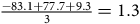
2. They can calculate the average on this encrypted data as
$${{ - 83.1 + 77.7 + 9.3} \over 3} = 1.3$$
as shown in Figure 5.Figure 4.How 3 parties, for example, insurance companies would build a federated machine learning model with a central body such as a regulator, reinsurer, professional body etc. aggregating encrypted model parameters. k denotes the training round number.
Figure 5.Example of how 3 insurers, labelled 0, 1, 2, could securely aggregate their private model parameters
$${\beta _0}$$
,
$${\beta _1}$$
,
$${\beta _2}$$
. Only pairwise noise is exchanged between them so no sensitive data leaves the insurers. The aggregating body receives only data with added noise so cannot infer anything about the parameters. However upon aggregating the data together the noise cancels out so the average can still be calculated without compromising the data.


We can prove this approach works if:
-
1. We let
$${{\rm{p}}_{{\rm{i}},{\rm{j}}}}$$
represent the particle sent from insurer
$${\rm{i}}$$
to insurer
$${\rm{j}}$$
-
2. Then each insurer
$${\rm{i}}$$
calculates
$${\tilde {\beta} _{\rm{i}}} = {{{\beta }}_{\rm{i}}} + \underbrace {\mathop \sum \nolimits_{{\rm{j}} \ne {\rm{i}}}^{\rm{n}} {{\rm{p}}_{{\rm{i}},{\rm{j}}}}}_{{\rm{Particle}}} - \underbrace {\mathop \sum \nolimits_{{\rm{i}} \ne {\rm{j}}}^{\rm{n}} {{\rm{p}}_{{\rm{j}},{\rm{i}}}}}_{{\rm{Antiparticle}}}$$
using their own private or sensitive data and resources i.e. without transferring any private data -
3.
$${\rm{C}}$$
then only receives
$${{{\tilde \beta }}_{\rm{i}}}$$
(and cannot deduce the value of any
$${{{\beta }}_{\rm{i}}}$$
) -
4.
$${\rm{C}}$$
then calculates the average model parameter
$${{\tilde \beta }}$$
as(1)
$${{\mathop \sum \nolimits_{i = 0}^n {{\tilde \beta }_i}} \over n} = {{\mathop \sum \nolimits_{i = 0}^n \left( {{\beta _i} + \underbrace {\mathop \sum \nolimits_{j \ne i}^n {p_{i,j}}}_{{\rm{Particle}}} - \underbrace {\mathop \sum \nolimits_{i \ne j}^n {p_{j,i}}}_{{\rm{Antiparticle}}}}\right)} \over n}$$


But by summing over
 $$i$$
, the particles
$$i$$
, the particles
 $${\mathop \sum \nolimits_{j \ne i}^n {p_{i,j}}}$$
cancel out with the antiparticles
$${\mathop \sum \nolimits_{j \ne i}^n {p_{i,j}}}$$
cancel out with the antiparticles
 $${\mathop \sum \nolimits_{i \ne j}^n {p_{j,i}}}$$
, “annihilating” each other, leaving us with:
$${\mathop \sum \nolimits_{i \ne j}^n {p_{j,i}}}$$
, “annihilating” each other, leaving us with:

The concept of incorporating particles and antiparticles, alternatively termed “one-time pad masks,” is attributed to Frank Miller (Bellovin, Reference Bellovin2011).
In our trivial example we only dealt with a single parameter
 $$\hat \beta $$
. But if a model were to use
$$\hat \beta $$
. But if a model were to use
 $$k$$
parameters say
$$k$$
parameters say
 $${\hat \beta _0},{\hat \beta _1},{\hat \beta _2}, \ldots, {\hat \beta _k}$$
, the exact same masking procedure can work on each parameter independently. One can simply in turn mask, and aggregate,
$${\hat \beta _0},{\hat \beta _1},{\hat \beta _2}, \ldots, {\hat \beta _k}$$
, the exact same masking procedure can work on each parameter independently. One can simply in turn mask, and aggregate,
 $${\hat \beta _0},{\hat \beta _1},{\hat \beta _2}, \ldots, {\hat \beta _k}$$
without any loss of generality.
$${\hat \beta _0},{\hat \beta _1},{\hat \beta _2}, \ldots, {\hat \beta _k}$$
without any loss of generality.
4.4.2. Practical Considerations
This relatively simple approach, or strategy, to securely aggregate the model parameters may not work very well if used for smartphone applications as was initially conceived by Google for several reasons:
-
1. Deep learning models often use a very large number of parameters. The GPT-3 model is said to use around 175 billion parameters (Floridi & Chiriatti, Reference Floridi and Chiriatti2020). Exchanging pairwise masks for billions of parameters, for millions of smartphones, would be incredibly inefficient and costly in terms of the amount of data needed to be exchanged.
-
2. As sending and exchanging model parameters costs data to transmit, and drains energy levels on smartphones, it tends to only occur when a sample of smartphones are plugged in to their charger and connected to Wi-Fi. However, smartphone users do not all charge their phones for the same length of time. Some will unplug their phone sooner than others. It is possible for a smartphone to be unplugged after they have sent their “Particles” and received their “Antiparticles,” but before they have sent their masked model parameters
$${{{\tilde \beta }}_{\rm{i}}}$$
to
$${\rm{C}}$$
. So the other smartphones will have sent parameters to
$${\rm{C}}$$
, but the dropped smartphones won’t send the corresponding cancellation figures, so the aggregation will fail e.g. a mask of +105 is sent to
$${\rm{C}}$$
but the −105 negative mask is never received to cancel it out. -
3. The potential millions of smartphone users building a FL will almost certainly be composed of strangers. There will not actually be a communication medium to exchange these pairwise particles between them as these strangers won’t have peer-to-peer communication set-up between them. A smartphone user does not generally exchange information (such as a particle) with an unknown smartphone user. Google thus proposed the use of a Diffie-Hellman key-exchange (Diffie & Hellman, Reference Diffie and Hellman1976) to allow users to indirectly talk to each other via the central body, without actually communicating with each other.


This led to Google improving the protocol outlined in Section 4.4.1 with their “Secure Aggregation” or SecAgg algorithm (Bonawitz et al., Reference Bonawitz, Ivanov, Kreuter, Marcedone, McMahan, Patel, Ramage, Segal and Seth2016). We do not believe these issues will materially affect insurance companies doing FL as they do in the case of smartphones given:
-
1. Insurance companies will have many more computational resources than individual smartphone users. Their computation would likely be carried out on much larger computers than smartphones, using computer servers, so the number of parameters should not be a limiting factor. It is also unlikely they would be concerned with the cost of transmitting the data as a large commercial entity.
-
2. For smartphones, FL involves millions of clients sharing a model. These clients do not generally talk to or coordinate with each other i.e. they could not feasibly guarantee all the smartphones will be plugged in and connected at the same time. In our application, we suggest a much smaller number of commercial enterprises would build a model together who would act very different to individual smartphone users. For example, in the UK Accident and Health Insurance market, as at 2019, the top 10 companies controlled 83.9% of the market (Guirguis, Reference Guirguis2019). Our study uses 10 companies as an example and we posit that these enterprises could freely communicate with each other. We propose they would all set a fixed date and time to commence FL. If any of the companies were to disconnect during training we posit that the companies could simply wait for them to rejoin or even restart the Federated Model building process. And as we believe insurance companies would quite happily talk and communicate with each other, this eliminates the need for a Diffie-Hellman key-exchange.
5. Experiment
5.1. Key Findings
We have attempted to model and predict (car) insurance claim frequencies on the widely studied freMTPL2freq dataset, available on OpenMLFootnote
1
using feed-forward artificial neural networks and data privacy preserving FL strategies. We considered 3 distinct scenarios. In all 3 cases, we have assumed there are 10 players in the market who each own
 $$1/{10^{th}}$$
of the industry’s claims experience. In each scenario, we test every model against a randomly selected unseen Test dataset, by measuring their exposure weighted percentage of Poisson deviance explained (%PDE). Our results show FL achieves nearly the same accuracy as if insurers were able to freely share sensitive customer data between them, but does not require data to be compromised.
$$1/{10^{th}}$$
of the industry’s claims experience. In each scenario, we test every model against a randomly selected unseen Test dataset, by measuring their exposure weighted percentage of Poisson deviance explained (%PDE). Our results show FL achieves nearly the same accuracy as if insurers were able to freely share sensitive customer data between them, but does not require data to be compromised.
-
1. Global Model Scenario
-
• Firstly, we consider a theoretical case where all the insurers work in total collaboration without any restrictions (legal, ethical, commercial or otherwise) on data sharing.
-
• In this scenario, we pool together all the data to one location and build a single predictive model using the entire industry’s data. As this model is built using the entirety of the data we refer to it as the “Global Model.” Each insurer uses this same model, so if not adjusted, they would give the same scores to every customer.
-
• We find that this model and approach is capable of explaining 5.57% exposure weighted PDE of the Test dataset.
-
-
2. Partial Model Scenario
-
• Secondly, and perhaps more realistically, we consider a case where insurers refuse to share any data with each other.
-
• Each of the 10 insurers independently builds their claim frequency model on their own. They will only have access to their own data – a partial subset of the entire industry’s claims experience. We therefore call each of these 10 models a “Partial Model.” No data is exchanged or shared between them.
-
• We find that out of the 10 models built by each insurer, no insurer can explain more than 3.82% exposure weighted PDE of the Test dataset, with the average performance of the 10 models to be 3.20% exposure weighted PDE.
-
-
3. Federated Model Scenario
-
• Finally, we consider a case where the 10 insurers refuse to share any customer data with each other, similar to the Partial Model approach. However, they agree to securely share and aggregate model parameters to build one shared Federated Model. As with the Global Model this Federated Model will be shared by all 10 insurers.
-
• We find that this model can explain 5.34% exposure weighted PDE of the Test data – significantly more than any of the Partial Models and slightly worse than if the insurers all agreed to share their data and build the Global Model.
-
This result indicates that insurance companies can effectively collaborate using the Federated Model approach to construct more predictive models, all without the need to directly share any customer data. Whilst our experience uses car insurance claim frequencies, the approach outlined here is applicable to any line-of-business, frequency or severity, or indeed any supervised learning task where data is limited and private.
5.2. Data
The freMTPL2freq car insurance claims data used for our experiment contains policyholder information such as driver age, vehicle age, and their number of third-party motor liability claims (which is the dependent y variable to be modelled) for a book of French car insurance business. Some brief data definitions are provided in Table 5 along with their preprocessing data transformations.
Description of data, fields, and preprocessing transformations used in experiment

We will treat this data as representative of some insurance risk that insurers may wish to model, which need not necessarily be third-party liability motor claims. For our purposes, the claims in the ClaimNb column of freMTPL2freq that we are aiming to predict, could represent motor, home, travel, sickness etc. insurance claims. The techniques presented here are agnostic to the line of business and we do not wish to focus on domain specific issues related to any particular insurance class such as motor liability. Our only requirement for the data is that insurers only have access to a small proportion of it, to ensure that every insurer participating in the Federated Model approach would stand to benefit similarly. The freMTPL2freq dataset will be thus treated as and assumed to represent the entire industry’s claims experience.
5.2.1. Test data
We hold back a random 20% sample of the data to serve as a Test set to evaluate all the models on. This data will not be used in any training or tuning of the models in any of the scenarios. Using this single shared Test data to evaluate all the models ensures the comparisons between the 3 modelling approaches are fair and consistent.
However, when building federated models in practice it may be difficult to produce such data. For example, perhaps
 $$n$$
insurers would all agree to withhold
$$n$$
insurers would all agree to withhold
 $$X$$
% of their Training data as Test. They might then all agree to collate these
$$X$$
% of their Training data as Test. They might then all agree to collate these
 $$n$$
sets of private Test data to one single shared Test data set, to collectively evaluate the performance of their shared Federated Model. This could raise similar challenges to those mentioned earlier. For instance, determining who would gather and manage these (Test) data could pose difficulties. Customers of one insurer may be hesitant to share their data with others, leading to potential legal and practical obstacles. In reality, having a single shared Test data may not be feasible. Instead, each of the
$$n$$
sets of private Test data to one single shared Test data set, to collectively evaluate the performance of their shared Federated Model. This could raise similar challenges to those mentioned earlier. For instance, determining who would gather and manage these (Test) data could pose difficulties. Customers of one insurer may be hesitant to share their data with others, leading to potential legal and practical obstacles. In reality, having a single shared Test data may not be feasible. Instead, each of the
 $$n$$
insurers would probably assess the performance of FL using their own distinct Test data, which they safeguard from other insurers to ensure privacy and security. Consequently, there would effectively be
$$n$$
insurers would probably assess the performance of FL using their own distinct Test data, which they safeguard from other insurers to ensure privacy and security. Consequently, there would effectively be
 $$n$$
Test data. However, for the sake of consistency in model comparisons, we maintain the same Test dataset across all experiments, preventing variations in model performance solely due to differences in random Test sets.
$$n$$
Test data. However, for the sake of consistency in model comparisons, we maintain the same Test dataset across all experiments, preventing variations in model performance solely due to differences in random Test sets.
5.2.2. Preprocessing and its Challenges
Once the training data is partitioned, we proceed to transform, scale, and preprocess the features, utilising only the Training data to derive the scaling parameters to prevent any leakage. We rely heavily on the work of Ferrario et al. (Reference Ferrario, Noll and Wuthrich2020) as a guiding framework for optimal treatment of variables, given their extensive study and modelling of this specific dataset. It is important to note that insurers typically would not have publicly shared research on their Training data. They would conduct their own comprehensive Exploratory Data Analysis (EDA) to derive the most appropriate transformations of their data. We rely on previously published analysis. The data preprocessing transformations used are given in Table 5 which take the number of explanatory columns to 39 after the dropping, encoding etc.
A crucial aspect of the presented Horizontal FL approach is the uniformity in feature usage, including preprocessing. For example, in our application all the insurers need to log transform the Density variable. If another insurer were to not scale Density or choose some other kind of transformation the parameter aggregation would not work. Therefore, it is essential for all insurers to reach a consensus on data transformation procedures before initiating FL. This requirement also implies that insurers cannot introduce their own custom features, a common practice in generalised linear modelling often used in the insurance sector. This requirement to use the exact same features, processed, and defined in the exact same way, may be difficult for insurers to agree on and should not be overlooked.
If the feature space of each agent is different e.g. one agent has data on age but not gender, and another has gender but not age, than an approach called vertical FL can be used. Whilst vertical FL can work with different features, or columns, of data, it requires that the rows of data between agents are linked. In our case this would mean that the agents have a mutually overlapping and intersecting set of policyholders which is not likely for insurers in the same line-of-business. Customers would not likely have multiple car insurance policies during the same exposure period from multiple insurers for example. Horizontal FL, which we use in this paper requires the opposite i.e. each agent possess the same columns as each other, but the rows (policyholders in this instance) are different. A vertical FL approach would be better suited to a cross-industry application e.g. a health insurer and pharmacy may have a customer on both their systems; both parties could benefit from sharing say their claims information and medicine purchasing history with each other to build a predictive model to forecast claims and sales.
Another interesting challenge is how to apply the MinMaxScaler in FL. This transformation needs to apply to the whole Training dataset. In this context, the 10 insurers must collectively determine the maximum and minimum values of DrivAge across all datasets. This shared knowledge is essential because each insurer must apply identical transformations to their respective datasets.
Example 5.2.2.1 Consider a scenario involving just two insurers, labelled as 0 and 1, with the following characteristics:
-
• Insurer 0’s youngest driver is 17 years old.
-
• Insurer 1’s youngest driver is 25 years old.
-
• Consequently, the minimum driver age across both datasets is 17.
Both insurers would need to scale their data using the minimum age of 17. Insurer 0 should not use their value of 25. However, insurer 0 may not want to, or be allowed to reveal their minimum driver age of 17 to insurer 1. This could also be considered sensitive data.
It is proposed that in practice companies may be willing to disclose the minimum and maximum driver and vehicle ages etc. without much data privacy or commercial risk. Insurers would likely not vary much in these domains. For example most car insurers would likely all have their youngest drivers as the youngest possible legal driving age in their market. It is also unlikely that much could be gleaned from knowing the oldest vehicle a competitor insures. It is unlikely that insurers will have wildly different minimum and maximums. Even if they did, it may not reveal much about their data. However, for a more robust approach, companies could use similar SMPC techniques in Section 4.3 to securely calculate the maximum and minimum of their data without revealing which insurer has the highest/lowest driver age etc. This is a similar problem to Yao’s Millionaire Problem whereby two millionaires wish to find out which of them is richer than the other. The challenge is how can they find the maximum of their wealth without telling the other millionaire what their wealth is.
Insurers could theoretically address this issue by utilising homomorphic encryption. This would involve encrypting the data in such a specific manner that would enable certain functions to perform calculations on the encrypted data, while still yielding the same output as if the unencrypted data has been used.
Example 5.2.2.2 For example insurer 0 and 1 from Example 5.2.2 could privately and individually encrypt their driver age data using a certain encryption algorithm. Say:
-
• Insurer 0’s youngest driver being 17 gets encrypted to an arbitrary value 649572
-
• Insurer 1’s youngest driver being 25 gets encrypted to an arbitrary value 587419
The function
 $$m\left( {a,b} \right) = min\left( {a,b} \right)$$
could clearly be run over the unencrypted values of 17 and 25 to give the correct answer. However this requires both parties (or an aggregator party) knowing and seeing the values of 17 and 25. Instead, they could both send in the values of 649572 and 587419 to a central body. For an appropriate choice of encryption method, there exists a certain function
$$m\left( {a,b} \right) = min\left( {a,b} \right)$$
could clearly be run over the unencrypted values of 17 and 25 to give the correct answer. However this requires both parties (or an aggregator party) knowing and seeing the values of 17 and 25. Instead, they could both send in the values of 649572 and 587419 to a central body. For an appropriate choice of encryption method, there exists a certain function
 $$h\left( {a,b} \right)$$
such that the central body could compute
$$h\left( {a,b} \right)$$
such that the central body could compute
 $$h\left( {649572,587419} \right) = 17$$
as required.
$$h\left( {649572,587419} \right) = 17$$
as required.
In other words,
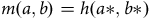 $$m\left( {a,b} \right) = h\left( {a{\rm{*}},b{\rm{*}}} \right)$$
where
$$m\left( {a,b} \right) = h\left( {a{\rm{*}},b{\rm{*}}} \right)$$
where
 $$a{\rm{*}}$$
and
$$a{\rm{*}}$$
and
 $$b{\rm{*}}$$
are encrypted values of
$$b{\rm{*}}$$
are encrypted values of
 $$a$$
and
$$a$$
and
 $$b$$
. This is the main idea of homomorphic encryption – to encrypt data in such a way that certain functions can output the same value as if they were computed on the raw data.
$$b$$
. This is the main idea of homomorphic encryption – to encrypt data in such a way that certain functions can output the same value as if they were computed on the raw data.
Using this we believe insurers could securely compute their combined minimum and maximum feature values for FL preprocessing. However, we consider homomorphic encryption beyond the scope of this paper. See Ertaul and Al-Azzawi (Reference Ertaul and Al-Azzawi2006) for more detail on how this technique works for computing minimum and maximum values.
There may also be some challenges encoding variables as well. For example consider how the insurers might encode a factor such as region or vehicle brand. This would entail the insurers agreeing to encode say brand name “B2” as a 1 in column number 30, “B3” as a 1 in column number 31 etc. or some other location in the data. All of the insurers would have to agree and use this exact encoding and transformation for FL to work. The insurers cannot use their own individual method to encode this factor. However this poses the question, how would they agree brand B2 belongs in column 30, B3 in column 31 etc.? The exact location (e.g. column number 30, 31 etc.) where the factor is encoded in the data is arbitrary, but the levels of encoding are not. For example if a more forthcoming insurer bravely suggests to their peers before building the FL model, that they use an encoding scheme such as: B2 belongs in column 30, B3 in column 31 etc. this may reveal to their peers that they insure B2, B3 etc. vehicles. Again, this could potentially be considered sensitive data to some degree depending on the feature. If they put forward how region might be encoded, it could reveal where they do and don’t write business. So the encoding strategy needs to be put forward in a way that doesn’t reveal anything. For example if encoding region, an insurer could propose an encoding strategy with reference to a public list, grouping, hierarchy, structure, or mutual definition, and suggest encoding levels whether or not they have any policies in those regions. The UK for example can be divided into 124 publicly known postcode areas, or France uses 18 administrative regions, or they could agree an area of more than
 $$X$$
square kilometres with a population of more than
$$X$$
square kilometres with a population of more than
 $$Y$$
according to the last known public census constitutes their modelling definition of “region.”
$$Y$$
according to the last known public census constitutes their modelling definition of “region.”
5.2.3. Splitting the Data Between Different Insurers
After separating the Test dataset from the rest, we uniformly and randomly split the freMTPL2freq data into 10 evenly sized sets, each containing an equal number of rows. This approach aims to simulate a scenario where each insurer possesses an equal share of the data. However, in real-world scenarios, such uniformity is unlikely due to several factors:
-
• The market is dominated by a single player that possess 80% of the data rather than
$$1/{10^{{\rm{th}}}}$$
of it. -
• Some of the insurers sell more business to certain types of car, businesses, buildings, sectors, customer ages, or to customers in certain regions.
-
• Some of the insurers enforce stricter underwriting than others and therefore have fewer claims in their data.

Instead of uniform allocation, stratified sampling could be considered, allocating more claims, data, or certain customer demographics to specific insurers. For simplicity, we overlook this complexity and assume a high degree of homogeneity among insurers.
Increased heterogeneity among insurers theoretically undermines the benefits of FL. Greater dissimilarities would necessitate tailored models for each insurer, reducing the advantages of aggregating model parameters. The more similar insurance companies and their data are, the more likely their models would benefit from FL. However, it is worth noting FL is frequently used in highly unbalanced and non-IID datasets. For example, when using smartphones for sentence prediction:
-
• Some users may contribute more text data than others, resulting in uneven data distribution among agents.
-
• Sometimes the model will be trained on a specific, biased, subset of users. FL training occurs at certain times of the day when phones are charging and connected to Wi-Fi. Training between 00:00–07:00 GMT time will train the models almost exclusively on British English, but will also be used by those speaking American English later on, leading to model bias.
Despite these challenges, Google’s original paper on FL found the protocol to be resilient against non-IID and imbalanced datasets, as demonstrated in their original paper (McMahan et al., Reference McMahan, Moore, Ramage, Hampson and Aguera y Arcas2017). Future research in this area could experiment with how more heterogeneous data splits (coupled with more complex aggregation strategies) could affect the results of this study.
5.2.4. Validation Data
After the data is split between the 10 insurers, we assume each insurer randomly selects 10% of their own data to use as Validation data to tune their models. As we are mimicking situations where each insurer holds a very limited amount of data they may not want to use too much of their data as Validation data. Insurers may also want to consider if any Validation data needs stratifying e.g. ensuring there are sufficient claims in the Validation as well as Training data.
5.2.5. Exploratory Data Analysis
Each insurer conducts Exploratory Data Analysis exclusively on their respective Training data. No party examines the Test or Validation data. Given our research’s primary aim to illustrate the practical implementation of FL, as opposed to prioritising the development of highly predictive models, our allocation of resources towards EDA is relatively conservative. Instead, we rely heavily on the work of Ferrario et al. (Reference Ferrario, Noll and Wuthrich2020) which has previously studied this data. In practice, insurers would not have previous academic research on their data, so EDA would be a crucial component of the modelling exercise.
Our limited EDA exercise in this section aims to simply show that the uniform sampling we have made between insurers unsurprisingly leads to insurers with similar data distributions. That is, no one insurer has materially more younger/older drivers, or one insurer has more/fewer claims than the others. Whilst FL can work on unbalanced and non-IID data (Bonawitz et al., Reference Bonawitz, Ivanov, Kreuter, Marcedone, McMahan, Patel, Ramage, Segal and Seth2016) our analysis here shows our exercise considers balanced data that appears to come from similar distributions between insurers. There does not appear to be any meaningful difference in any of the 10 agent’s explanatory variables. Figure 6 illustrates dissimilarities observed within insurers 8 and 9 where they do not have policies that have 4 claims. Conversely, a relatively uniform distribution of claim counts is evident across all 10 agents. Figures 7, 8 and 9 reveal negligible disparities in distribution patterns among the 10 agents.
Distribution of Number of Claims and Exposure.

Distribution of Vehicle Power and Age.

Distribution of Driver Age and Bonus Malus.

Distribution of Vehicle Gas and Vehicle Density.

5.3. Global Model Scenario
In this instance a single central entity has access to all of the Training and Validation data. We will use all of this data to build and tune the “Global Model.”
5.3.1. Model Design, Architecture, and Tuning Search Space
In all 3 scenarios we will fit a feed-forward artificial neural network multilayer perceptron to the data using the PyTorch package in Python. Every model will use the same architecture given in Table 6. We will use a Random Grid Search to tune only the learning rate, batch size, neurons in layer 1 and neurons in layer 2 considering 40 possible hyperparameter configurations given in Table 7.We note that whilst NAdam does adaptively tune the learning rate we do find some improvement over its default by slightly tuning this hyperparameter who’s default originated from computer vision tasks rather than regression (Dozat, Reference Dozat2016).
Neural Network Architecture used in all 3 Scenarios

Hyperparameter Search Space Considered in all 3 Scenarios

5.3.2. Global Model Hyperparameter Tuning And Test Results
The results of the top 5 Global Model hyperparameter tuning combinations are given in Table 8. We find using a batch size of 5,000; 15 neurons in the first hidden layer; 10 in the second; and a learning rate of 0.01 explains the highest amount of Validation exposure weighted PDE, leading to these hyperparameters being selected for the Global Model.
Top 5 hyperparameter sets for the Global Models

We see that the Global Model fits the Training data better than the Validation data due to generalisation error as expected. For the best performing set of hyperparameters this drop in performance is relatively small, indicating the model is not significantly overfitting. After selecting the hyperparameters, the Global Model is retrained using the entire combination of both the Training and Validation datasets. No data outside of the Test dataset is unused to train the model.
We find after hyperparameter tuning the Global Model achieves a 5.57% exposure weighted PDE and a 0.2956 Gini. This is a similar level of performance achieved on this dataset in Mayer and Lorentzen (Reference Mayer and Lorentzen2020).
5.4. Partial Model Scenario
Under this scenario we assume 10 insurers act totally independently. They do not share any data with each other and each try to build the best model they can, using only the data that they themselves possess. We will use the same model design, architecture, and tuning search space as in the Global Model scenario in Section 5.3.
5.4.1. Partial Model Hyperparameter Tuning And Test Results
We show each agent’s best chosen hyperparameters in Table 9. As per the Global Model, each agent refits their final chosen model using both the Training and Validation Dataset. No data is shared between agents in this scenario, including any results of hyperparameter tuning. Insurance company
 $$i$$
does not know what insurance company
$$i$$
does not know what insurance company
 $$j$$
gets on their Validation loss for a given hyperparameter set, to ensure privacy is maintained and one insurer cannot infer data from another based on hyperparameter tuning results.
$$j$$
gets on their Validation loss for a given hyperparameter set, to ensure privacy is maintained and one insurer cannot infer data from another based on hyperparameter tuning results.
Chosen hyperparameters of each insurer using just their own private, unique data

The results of each insurer’s performance against the Test set are given in Table 10. We can see that when acting individually each agent performs significantly worse than the Global Model on the test as one might expect. Each agent only has access to 10% of the Global Model’s data. The best performing agent can only score 3.82% exposure weighted PDE on the Test set, achieving 68.57% of the Global Model’s performance. We summarise the agent’s performance as a boxplot in Figure 10. The Global Model’s Test performance is included in the boxplot for comparison purposes only – it is not an outlier with respect to the agent’s performance.
Performance of each insurer’s model against the Test set using just their own private data

Box plot of each insurer’s performance on the test set using just their own private data. The Global Model performance is also shown here for reference and is not an outlier. We can see that none of the insurers acting individually can approach the performance of the Global Model where data was freely shared between them.

5.5. Federated Model Scenario
Under this scenario we use the same initial set-up as in Section 5.4. 10 agents will all possess the exact same data (which is a randomly selected 10% of the entire dataset). They will not share or transfer any private data between them unlike the Global scenario, but as per the Partial scenario they will keep their customer data to themselves. They will use the same model architecture and hyperparameter search space as in Section 5.4 and 5.3 with the exception of the number of epochs which we will discuss in Section 7.3. They will agree to keep all their private data on their own servers and infrastructure. However, they will securely share model weights to collectively build a shared Federated Model which they can all use to make model predictions.
5.5.1. Federated Model Hyperparameter Tuning And Test Results
FL poses a unique challenge in hyperparameter tuning. We propose a novel method using SMPC which insurance companies could use in Section 7, with the results of the top 5 shown in Table 11.
Top 5 Results of the novel hyperparameter tuning method proposed in Section 7

FL learning rate and Local Validation Loss

Our approach uses the average hyperparameter tuning results from the Partial Model scenario. We find that, on average across the local agents, 0.001 learning rate coupled with using 15 neurons in layer 1, 5 in layer 2 and a batch size of 500 appears to be the best combination. We thus select these for the Federated Model’s hyperparameters. We can see in the Partial model scenario no insurer found this selection to be their own unique private best set of hyperparameters i.e. left to their own devices these particular hyperparameters would be suboptimal, so this may be an area of compromise between them.
Unlike the Global and Partial scenarios, we also need to specify the number of rounds and local epochs which we set to 300 and 10 respectively. We provide more details of these hyperparameters in Section 7.3. A more precise description of the FL hyperparameters selection is given in Section 7).
We find that the Federated Model achieves an exposure weighted PDE% of 5.34% on the Test data set, significantly higher than any of the individual insurers working alone in the Partial scenario. Importantly, we observe the Federated Model achieves model performance slightly below the Global model, which we consider an “upper limit” in this study of what is achievable in terms of model performance. The Federated Model achieves nearly the same performance as if the insurers freely shared their data with each other, whilst keeping it private. We graphically compare the results of all 3 approaches finally in Figure 11.
Comparison of the performance of the 3 modelling approaches on the Test set. Using only the data available to each insurer leads to very poor performance, as shown in the boxplot compared to the either completely sharing the data with each other, or using FL. We can see that FL achieves nearly the same model performance as if the insurers were to completely share their sensitive data.

6. Results Analysis
We can see that the Federated Model achieves a lower, albeit, similar test performance to the Global Model. In Figure 12 we show a double lift chart comparing these 2 models, which demonstrates how the Global Model predicts the Test set better. Whilst both models over and under predict claims for certain customers, we can see the Global Model’s predictions are closer to the actual number of claims than the Federated Model. However, the Global Model’s performance can only be achieved if the insurers were to freely share all their data amongst them.
Double lift chart comparing the performance of the Federated Model against the Global Model on the Test dataset, with the Global Model showing slightly better performance than the Federated Model. The “X” shape by the orange and green lines show model performance by the 2 models is fairly even.

In a more likely scenario insurance claims data would not be shared and each insurer would have to rely on their own private data, to build their own partial individual model. In Figure 13 we show a double lift chart comparing insurer 5’s model against the Federated Model – insurer 5 being the insurer with the best scoring Partial individual model on the Test set. This chart shows agent 5 is significantly more accurate in predicting claims by using FL, without having to compromise and share its sensitive data.
Double lift chart comparing the performance of the Federated Model against agent 5 on the Test data set. The Federated Model shows significantly higher model prediction accuracy compared to just using agent 5’s own data. Unlike the Global Model versus Federated double lift, the green and orange lines do not show a symmetrical “X” shape. The green line showing the Federated Model’s prediction lie significantly closer to the actual claims on the blue line.

Compared to using the Federated Model we can see that they could over predict claims by more than 125% for some customer segments, likely leading to them massively overcharging and as a result losing customers. On the other side we can also see agent 5’s model under predicting claims by nearly 40%, which would lead to under-pricing these customers. We can see this in Figure 14 which shows the claims predicted by the Global Model (red line), and by the Federated Model (green line) match the actual claims (blue line) fairly well. However agent 5 (orange dotted line) appears to over predict claims for all areas indicating a very poor fit. We also show the Gini coefficient of each model in Figure 15, which shows that the Federated Model is almost as accurate as the Global Model at ranking customers. Whilst it does not reach as high a Gini coefficient we can see that it still outperforms all agent’s models in terms of ranking ability.
Actual versus expected of Federated, Global, and the best performing individual insurer (agent 5) by Area, showing that whilst the Federated and Global Model predict the actual claims fairly well (being close to the blue line), agent 5’s model using just their own data leads to predictions that are too high.

Gini index by model demonstrating each model’s ability to rank policyholders correctly in terms of their relative risk to one another. We can observe that as with the Poisson deviance the Federated Model achieves similar performance to the Global but the Partial Models do not perform as well on this metric either. The “Oracle” shows the theoretical perfect model that would rank policyholders in perfect order without any error and included for benchmarking.

7. Federated Hyperparameter Tuning
As discussed in Section 5.5.1 tuning the Federated Model hyperparameters requires a particular approach not found in the other scenarios. The choice of hyperparameters is usually done by selecting the set of hyperparameters that maximises or minimises some relevant metric on some kind of Validation dataset. However, the Validation data and performance of a particular set of hyperparameters is also sensitive data that should not be centralised. This presents a unique challenge to tuning the Federated Model.
Example 7.1 Consider a case where 2 insurance companies (Insurer A and Insurer B) wish to tune their Federated Model’s learning rate. Let us assume they wish to choose between 0.01 and 0.001. They could try training a Federated Model on both these hyperparameters, and each could measure some kind of Validation loss. Suppose for this they observe as per Table 12:
This would lead them to use the 0.001 rate.
The insurers would need to compute the average Validation loss for the 0.01 and 0.001 learning rate in order to compare which hyperparameter fits their data better (on average), as in Table 13:
FL learning rate and Average Local Validation Loss

FL Local Learning Rate and Local Validation Loss

This would lead them to use the 0.001 rate.
However, we find 3 problems:
-
1. Insurer A and B must not see each other’s Validation loss. Just like sharing unencrypted model parameters, the results of hyperparameter tuning could be sensitive data. Observing how another agent’s model performs under different hyperparameters could imply how their data are structured. It may be possible to infer if another company has higher or lower claims as they add more neurons or layers for example. Thus Table 13 cannot be observed by any party. We will thus have to employ some form of SMPC like those outlined in Section 4.3 to securely aggregate the results.
-
2. Due to the added complexities of encrypting and securely aggregating the parameters not present in traditional methods, Federated Models can take substantially longer to train and fit than training traditional ML models. Tuning can thus be very time-consuming for large grids. Therefore we seek to avoid wasting resource training Federated Models that will not be used (like the 0.001 learning rate in this example).
-
3. Hyperparameter optimisation can be sped up with algorithms like Successive Halving (Karnin et al., Reference Karnin, Koren and Somekh2013) or HyperBand (Li et al., Reference Li, Jamieson, DeSalvo, Rostamizadeh and Talwalkar2018). However common Python hyperparameter optimisation packages like Scikit-learn (Pedregosa et al., Reference Pedregosa, Varoquaux, Gramfort, Michel, Thirion, Grisel, Blondel, Prettenhofer, Weiss, Dubourg, Vanderplas, Passos, Cournapeau, Brucher, Perrot and Duchesnay2011) or Optuna (Akiba et al., Reference Akiba, Sano, Yanase, Ohta and Koyama2019) do not currently integrate easily with FL packages. They are not currently built with the encryption and secure aggregation functionalities required for FL.
7.1. Proposed Federated Learning Hyperparameter Protocol
We thus propose a novel approach. Rather than tune the hyperparameters of the Federated Model itself, it may be quicker and practically easier for each insurer to first tune their own local models independently i.e. build their Partial Models. Indeed, even when doing FL, in practice it is likely each insurer would still build their own internal private model in any case to test and trial against the Federated Model.
We suggest the same steps performed in Section 5.4 are performed at first, with each insurer tuning and finding their own set of hyperparameters on their own local data. The local hyperparameter tuning results of each insurer can then be used to set the Federated Model’s hyperparameters.
Example 7.1.1 Let us imagine the same set-up as in Example 7.1 but without any kind of FL. In this example, insurers A and B want to fit their own learning rate to their own data. This is essentially the same case as the Partial Model scenario in Section 5.4. See Table 14.
Unlike Example 7.1 this would:
-
• Be easily implemented in many open-source packages
-
• Not require any encryption aggregation steps – leading to significantly faster computation
It is then relatively easy to implement a SMPC protocol as outline in Section 4.3 to compute the average of 0.18 and 0.12, and 0.63 and 0.22, even using open source. Both insurers could then produce the results in Table 15.
FL Local Learning Rate and Average Local Validation Loss

We in essence suggest picking the hyperparameters that, on average, fit the Partial Models best, rather than the hyperparameters that actually fit the Federated model best, due to computational difficulties. This approach also has further benefits including:
-
1. Insurers can locally use whatever hyperparameter tuning framework they wish
-
◦ A simple RandomGridSearch from Scikit-learn or State-of-the-Art Tree of Parzen Estimators (TPE) from Optuna can easily be integrated with this approach, allowing each insurer to at least locally find a suitable set of hyperparameters. This approach works with either framework as long as the results of hyperparameter tuning are saved, and each insurer considers the same hyperparameters.
-
◦ However, it may be difficult to compare different insurer’s hyperparameter results if employing some kind of search algorithm with pruning or exploration. For example if 9 out of 10 insurers all prune networks with say more than 3 layers, but 1 insurer experiences very low loss with more than 5 layers, then the other insurers will not want to use this architecture when they have never even tested such a hyperparameter set up.
-
◦ It may be necessary then to modify this approach to only consider mutually tested hyperparameters. For example, perhaps any hyperparameter set needs at least 50% of the insurers to have explored and tested it. So, in the above point the 5 layer network (tested by just 1 insurer) wouldn’t meet the criterion.
-
-
2. Computational Efficiency
-
◦ As a byproduct of this approach, insurers will get their own unique private model. Even when doing FL it is likely that insurers will still want their own internal model to test against. They would likely want to A/B test the Federated Model against their own Partial model to see which is more accurate in practice.
-
◦ Or flipped around – insurers may already have local hyperparameter tuning results from models they have already built that this method can leverage off. Even when doing FL it may be a natural first instinct to still try and build a local model on whatever data is available. This would serve as a starting point to see its performance, before trying to collaborate with other parties first.
-
7.2. Limitations of approach
However this approach relies on a critical and hard to prove assumption – that the local optimal hyperparameters are the same (or similar) to the Federated Model’s optimal hyperparameters. Observe in Example 7.1 when the Federated Model was “fully” tuned (which would be computationally and technically challenging) that the ideal learning rate was found to be 0.001.
If insurers instead implement our approach in Example 7.1.1 they would unfortunately select a suboptimal learning rate rather than the “correct” one. But insurers would have no way of knowing or verifying the key assumption without actually doing the federated tuning which this method seeks to avoid. It is practically difficult to prove this assumption. For the likely circumstances of how we envisage this method being used (bearing in mind the number of insurers, volume of data, model forms etc.). We therefore assume this is not an unreasonable a priori assumption. We are in essence assuming that if insurers find a certain number of neurons, layers etc. that fits their own limited data well, then it will fit the entire data well too.
Formalised Expression Of Proposed Federated Hyperparameter Tuning Protocol

7.3. Federated Communication Rounds and Local Epochs Hyperparameters
Another unique facet of the federated scenario is the number of communication rounds, which is the number of times the agents average their weights together. Recall that in FL each agent goes through cycles of training their model locally, then sending their parameters, and receiving new average parameters. Figure 4 showed what this would look like with 2 communication rounds.
More communication rounds means more averaging of the parameters between the agents. This hyperparameter is akin to epochs in a traditional deep learning modelling approach. Every rounds is a (federated) update to the neural network’s weights and biases. Much like epochs, too many rounds could lead to overfitting, and too few could lead to underfitting. No insurer has a concept of rounds on a local, traditional deep learning, basis. They can only train their own partial model for a certain number of epochs. We thus cannot use the proposed method in Section 7.1 to select the appropriate number of rounds as it has no analogue in the Partial scenario. Instead we propose insurers would have to use a method of tuning similar to Example 7.1. That is, they would have to:
-
1. Try training different Federated Models with a varying number of rounds.
-
2. Each of the 10 agents would record their own private validation performance on each of these Federated Models.
-
3. For each of these Federated Models trained with a different number of rounds the 10 insurers would have to securely compute the average Validation performance between them using a SMPC method outlined in Section 4.3.
-
4. The 10 insurers would then select the Federated Model trained with the number of rounds that experienced the best average Validation performance between them.
Again this approach may be difficult to agree in practice if each insurer finds a particular number of rounds fits their local validation data a lot better than the average selected number of rounds. In our experiment we consider the 10 insurers training their Federated Model 250, 300, and 350 rounds, before testing on their Validation data individually. We show the average validation performance of each of these rounds in Figure 16 which shows 300 to be the optimal number on average which we assume the insurers can compute securely between them. We can see that the Federated Model improves with more rounds up until 300, whereby more rounds appears to lead to overfitting and worse validation performance. After selecting the number of rounds the Federated Model is then re-trained using 300 rounds on all of the insurers training and validation data.
Average validation performance of the Federated Model against various different numbers of rounds. We can see performance begins to decrease after 300 rounds so we assume the insurers would select this as the optimal amount of training.

(a) Graph showing training times of each model rebased to the Global Model training time. (b) Exposure Weighted Validation % PDE of the Global and Federated Models over different number of parameter update steps. Comparison of Federated Model training times. Whilst the observed wall time for FL appears to be longer in a) this may be due to federated learning requiring more update steps to reach the optimal set of parameters as shown in b).

As well as setting the number of rounds, the Federated Model must also assume a local number of epochs. Recall that every time an insurer receives an updated Federated Model, they need to re-fit this Federated Model to their own data. To fit this Federated Model to their own data, they need to select how many epochs are required for the local training steps.
The main idea of FL is that locally each agent possesses little data, so it may make sense to use a low number of local epochs as to avoid overfitting before broadcasting. In this scenario we suggest that insurer trains their model for just 10 local epochs before they (securely) broadcast their parameters. As with the number of rounds this hyperparameter can be tuned in the same way if required.
8. Further Considerations for Federated Learning
8.1. Regulation
FL is an innovative approach that could assist practitioners to adhere to current data protection regulations, including the EU GDPR, as multiple participants collaboratively train a model, ensuring that their data remains decentralised and private. Further, by processing data at its source, FL enhances privacy. This decentralised training could fast become the standard for handling and storing private data, particularly in a world where privacy concerns are paramount (Fernandez et al., Reference Fernandez, Brennecke, Barbereau, Rieger and Fridgen2023).
The EU GDPR emphasises principles such as data minimisation, purpose limitation, and user consent. Organisations implementing FL should ensure compliance with such regulations and consider incorporating other privacy-enhancing techniques like differential privacy. Transparency and explainability are also becoming important considerations. As FL involves multiple participants contributing to a model, it is crucial to establish clear guidelines and transparency around how the model is trained, how data are collected, and how decisions are made.
Regulations increasingly seek to address issues related to model biases, fairness, and accountability. As FL relies on diverse datasets from different sources, it is essential to ensure that biases are carefully identified, measured and mitigated to prevent any discriminatory outcomes. Because FL involves combining more diverse data, biases may be easier to address than in a centralised approach. However, bias propagation could occur in FL if participants could potentially influence all parties in the network, thus aggravating the fairness problem globally (Chang & Shokri, Reference Chang and Shokri2023) as mentioned in Section 4.1. For example, when Google first launched FL for text prediction for Android mobile devices, model training occurred nightly at a specific time, when devices were idle and plugged in. This meant that the data was from the same timezone and used the same language, i.e. training could have been done for devices using English in the US and hence the text prediction would not have accounted for nuances in how English is used across other English speaking nations (McMahan & Ramage, Reference McMahan and Ramage2017).
8.2. Federated Learning Ecosystem
FL is still a relatively new modelling approach and there are many different packages and implementations for practitioners to utilise, each of which will have various pros and cons.
It is difficult to choose the best framework given FL is a nascent technology. We initially started with PySyft but found that, whilst it worked well with theoretical examples, it struggled to implement FL it in practice. We chose the Flower (Beutel et al., Reference Beutel, Topal, Mathur, Qiu, Fernandez-Marques, Gao, Sani, Kwing, Parcollet, Gusmão and Lane2020) framework ultimately as it worked well in practice. It is worth noting this research used Flower version 1.1.0 which does not come with SMPC built in. However the Flower package is very adaptable, which allowed us to implement and plug in our own SMPC protocol which we coded in Python from first principles.
8.3. Hyperparameter Tuning
Tuning hyperparameters is an important but tedious part of the machine learning pipeline, and this is no different for the FL paradigm. However, hyperparameter optimisation cam be even more challenging in FL. In federated networks, Validation data is distributed across devices, preventing the entire dataset from being available simultaneously (if any exists at all – recall FL is used in times of data sparsity). Below are some FL specific hyperparameter tuning approaches that have been proposed:
-
1. FedEx, can be used to accelerate federated hyperparameter tuning by alternating the minimisation of weights with exponential updates of the standard SGD algorithm which can lead to quicker convergence (Khodak et al., Reference Khodak, Tu, Li, Li, Balcan, Smith and Talwalkar2021).
-
2. Bayesian optimisation can also be used with FL via Thompson sampling (which reduces the number of parameters needed to be communicated between clients) whereby a prior distribution e.g. Gaussian is assumed, whilst ensuring convergence. This can be further extended with distributed exploration, whereby local agents will search for their own local optimum at initialisation (Dai et al., Reference Dai, Low and Jaillet2021).
In this paper, we have also implemented a novel hyperparameter tuning protocol, whereby all insurers would agree on a shared hyperparameter search space and a minimum global Validation Loss parameter could be computed to optimise hyperparameters.
8.4. Training Times
Whilst this paper finds that FL can achieve near the same model performance as if data were freely shared between insurers, this does come at the expense of a large increase in training times. We have used the Skorch (Tietz et al., Reference Tietz, Fan, Nouri and Bossan2017) package in Python to perform hyperparameter optimisation for the Local and Global models using random grid Searching. For each set of potential hyperparameters Skorch records the wall time taken to fit the model, using just the Training data (the models ultimately used for Test evaluation are refit using Training and Validation data). We compare the time taken to train the Federated Model, the average time taken to train each of the 10 Local models, and the Global Model, in Figure 17(a). As expected, the Partial Models take approximately 10% of the time to train compared to the Global Model, as they effectively split the data into 10 chunks and train 10 models in parallel. However the Federated Model takes about 2.5 times longer to train than the Global Model. This comparison is not quite like-for-like however. Recall that the Federated Model is trained for 300 rounds of 10 local epochs. This is essentially
 $$300{\rm{*}}10 = 3000$$
parameter update steps coupled with encrypted averaging computations. Meanwhile the Global and Local models both used 10 times fewer updates by just using 300 epochs.
$$300{\rm{*}}10 = 3000$$
parameter update steps coupled with encrypted averaging computations. Meanwhile the Global and Local models both used 10 times fewer updates by just using 300 epochs.
During the final fitting of the Global and Partial Models (using both the Training and Validation data) Skorch records the (exposure weighted) percentage PDE of the models against the Validation data at each epoch. As these models are trained using Validation data, and the metric is calculated against Validation data, it does not indicate model performance. However, it can be used to observe if the model parameters are converging by observing any plateaus which indicate the model’s optimiser is no longer substantially updating weights and biases. We can see in Figure 17(b) that training the Global Model for more than around 250 parameter update steps leads to relatively little or no change in model parameters. In contrast the Federated Model still benefits from training until around 2,500 parameter update steps. The additional encryption mechanisms of FL may thus not be increasing the training times of the model substantially. The observed longer times may instead be due to the model needing more parameter update steps. This could be a facet of the simple federated averaging aggregating process we use here, where we spread and average out the updated parameters of the federated neural network. This process may be inefficient compared to the parameter updates used in the Global and Local Models.
8.5. Sustainability
Sustainability and climate change is a key consideration when training ML and FL models as these infrastructures use great amounts of energy and specialised hardware, which in turn generates carbon emissions. Traditional AI training methods require vast amounts of data to be transmitted to and processed by centralised data centres.
Further, it is possible that FL training could emit less carbon than data centre GPUs even though FL models take longer to converge. However, this observation was noted to be highly sensitive to the data used for training as well as the ML setting (Qiu et al., Reference Qiu, Parcollet, Beutel, Topal, Mathur and Lane2021). Further research also suggested other forms of consensus driven distributed FL that could potentially reduce energy consumption on the server side (Savazzi et al., Reference Savazzi, Rampa, Kianoush and Bennis2023).
8.6. Adversarial Attacks
Ensuring FL training is secure against adversarial attacks is key to ensuring participants trust the decentralised ecosystem. There could be risks of poisoning attacks (Jere et al., Reference Jere, Farnan and Koushanfar2021), whereby some unethical companies could report anomalous results leading to inaccurate FL results. Further, bad actors could monitor how the FL subsequently updates its parameters, they could potentially infer the claims frequencies of the other insurers (Rodríguez-Barroso et al., Reference Rodríguez-Barroso, Jiménez-López, Luzón, Herrera and Martínez-Cámara2023). This means it is key to ensure all FL participants are trustworthy partners.
The study of adversarial attacks to FL is an ongoing field of study which is becoming increasingly important as it helps ensure FL remains a robust machine learning technique that safeguards data privacy. By the nature of how FL is being run, where there are many distributed underlying data systems and centralised aggregation servers, these could make the infrastructure more vulnerable to potential cyber crime.
8.7. Use of Neural Networks Compared to Other Modelling Methods in FL
FL was initially implemented for non-tabular data related tasks such as text prediction or image recognition on smartphones. As such it has historically focused on deep learning methodologies, where this approach excels. However whilst deep learning has made great strides in the world of AI, GBMs have typically outperformed them on most tabular regression tasks which are common to actuarial work. This has been the case in many Kaggle’s competitions (Carlens, Reference Carlens2023). Grinsztajn et al., (Reference Grinsztajn, Oyallon and Varoquaux2022), Shwartz-Ziv and Armon (Reference Shwartz-Ziv and Armon2021), and Popov et al., (Reference Popov, Morozov and Babenko2019) have discussed possible reasons driving this phenomenon. Industry surveys also show little use of deep learning in actuarial science by practitioners (Rioux et al., Reference Rioux, Da Silva, Jones and Saleh2019 and Nocon et al., Reference Nocon, Mathieson, Allenby, Crawford, Day, Jarvis, Johnson, King, Murphy, Russell, Tam and Yao2017).
FL can be extended to gradient boosting machines. One natural way is to consider each agent computing the gradients of a particular tree that’s part of the Global GBM. These can be aggregated using some form of SMPC by a central body. This is the approach taken by Tian et al., (Reference Tian, Zhang, Hou, Lyu, Zhang, Liu and Ren2024) which they called FederBoost, however, as the decision tree grows, each node naturally possesses less and less data. This leaves this approach exposed to some privacy leakage as explained in Yamamoto et al., (Reference Yamamoto, Ozawa and Wang2022) and is computationally expensive. Alternatively, rather than each agent considering a Global GBM that they all try to build together, they could each simply build their own set of local trees on their own. As these would be built on their own limited data we can consider them weak learners like trees in a random forest. These local trees then need some form of secure aggregation. A sequential boosting aggregation based approach is described in Zhao et al. (Reference Zhao, Ni, Hu, Chen, Zhou, Xiao and Wu2018) which can address some of the privacy concerns of Tian et al., (Reference Tian, Zhang, Hou, Lyu, Zhang, Liu and Ren2024) at the expense of some model accuracy. Another potential approach is to combine each agent’s weak set of trees by securely bagging their predictions which can be implemented in Flower and Nvidia’s FLARE (Roth et al., Reference Roth, Cheng, Wen, Yang, Xu, Hsieh, Kersten, Harouni, Zhao, Lu, Zhang, Li, Myronenko, Yang, Yang, Rieke, Quraini, Chen, Xu and Feng2022) package.
In practice many insurers will still use GLMs (Baribeau, Reference Baribeau2017) for actuarial modelling due to their ease of deployment and explainability or even regulation. As outlined in Section 3.2 we can however easily configure the approach given in this paper to apply to GLMs by considering them to be a special case of a NN.
9. Conclusion
FL is a new machine learning research area which has contributed greatly to many industries, for example enabling mobile phones to collaboratively learn a shared prediction model whilst keeping all the Training data on personal devices. In our paper we simulate (motor) insurers openly and freely sharing private and sensitive customer data with each other to build an actuarial claims prediction neural network model. We find that the same insurers could build a model with nearly the same performance using FL that would take significantly longer to train. However by using FL these insurers would not need to share any of their sensitive customer data. The small drop in model performance, and large increase in training times, may be a worthy trade for insurers to increase the accuracy of their predictions whilst keeping their customer data private. Whilst our results show a great deal of promise for the potential of FL in insurance, numerous challenges still exists such as best practice, training times, regulation, and expertise in this area. However, given the insurance industry’s history of pooling data and risk together, FL should be an area of continued development.
Acknowledgement
The Institute and Faculty of Actuaries (IFoA) Federated Learning Working Party would like to thank the IFoA for the continued support in this research. We would like to express our gratitude to Claudio Giancaterino for his valuable contributions to this project, and the Flower development team for their support and guidance.


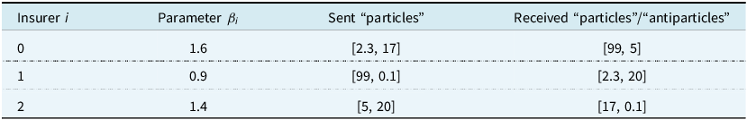

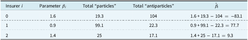


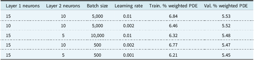


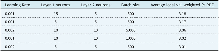

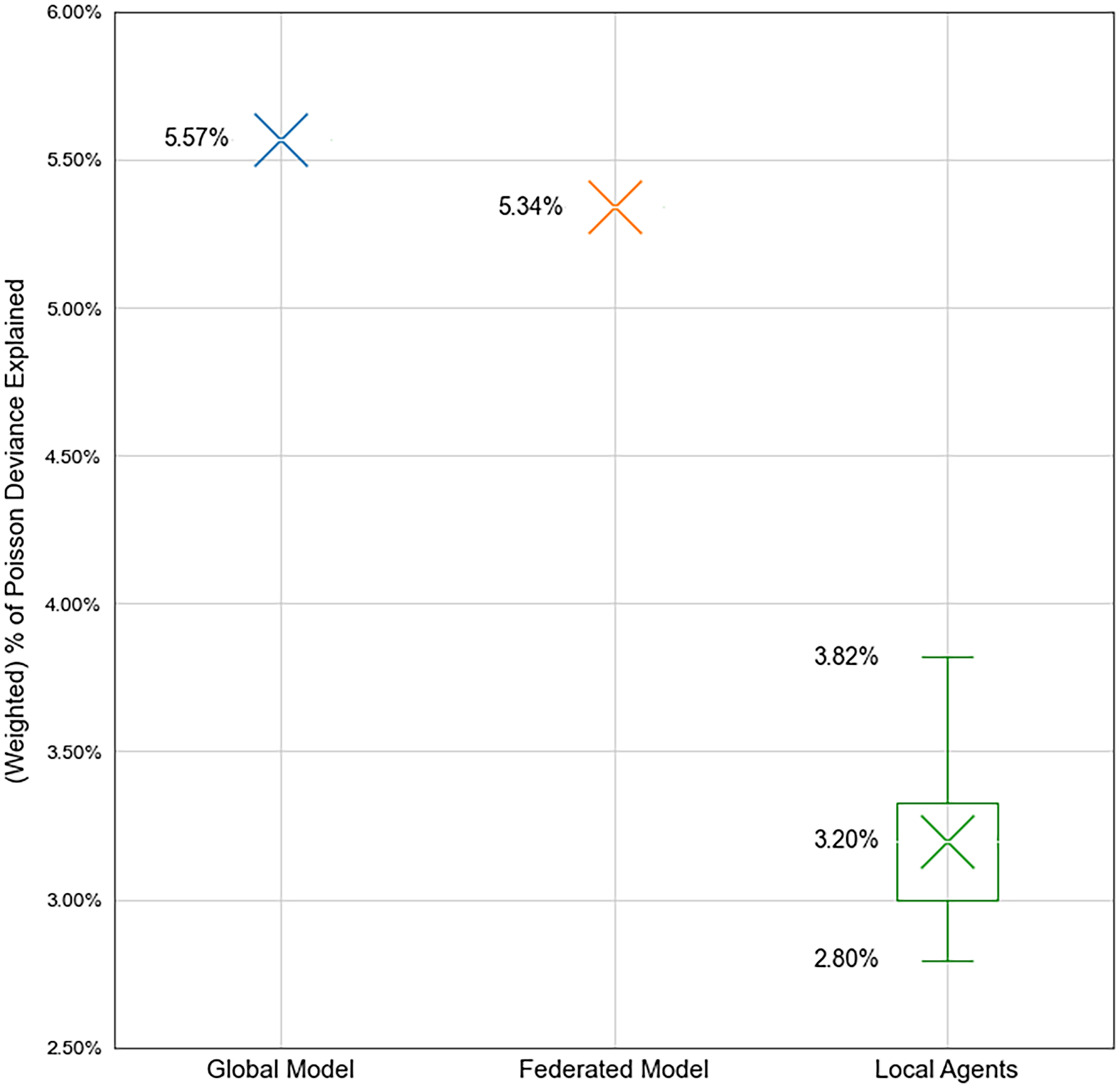


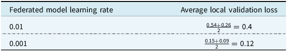


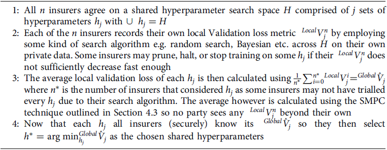


 Open access