1. Introduction
The base of a glacier or an ice sheet is notoriously difficult to access. Basal boundary conditions are therefore usually unknown. Unfortunately they determine, to a large part, the total discharge and flow behavior of the ice. It is therefore desirable to try to infer the basal boundary condition from measurements that can be made on the surface or from air- or space-borne platforms, namely ice depth and surface topography and velocities.
Various methods for solving the inverse problem to compute basal boundary conditions exist. They depend on the physical situation that is being addressed and often rely on a simplified treatment of the full three-dimensional (3-D) Stokes equations (i.e. the momentum balance equation neglecting accelerating terms; Reference HutterHutter, 1983). Reference MacAyealMacAyeal (1992) pioneered the use of formal inverse methods in glaciology to infer basal drag under ice streams using a zero-order model based on shallowness (see also Reference MacAyealMacAyeal,1993; Reference Joughin, MacAyeal and TulaczykJoughin and others, 2004).
On the other hand, it is possible to calculate transfer functions for variations of bed topography and slipperiness to the ice surface (e.g. Reference Raymond and GudmundssonRaymond and Gudmundsson, 2005) and to use linearized transfer functions to estimate bed properties from surface measurements (Reference Thorsteinsson, Raymond, Gudmundsson, Bindschadler, Vornberger and JoughinThorsteinsson and others, 2003). Other applications include the derivation of basal velocities along longitudinal profiles based on longitudinal averaging (Reference TrufferTruffer, 2004) or on a first-order forward model and a Monte Carlo inversion (Reference Chandler, Hubbard, Hubbard and NienowChandler and others, 2006).
Here we also consider a simplification to the general Stokes equations for an incompressible fluid (Reference LliboutryLliboutry, 1987, section 6.2). Following Reference LliboutryLliboutry (1987, ch. 7), we treat isothermal flow through a valley glacier’s cross-section under the simplifying assumption that the in-plane velocity components and all out-of-plane gradients are zero. That is, in a coordinate system with z pointing out-of-plane along the mean down-glacier slope, y perpendicularly upwards and x across the glacier, we assume that the velocity vector u = (0, 0, u) T has only one non-zero component and all derivatives ∂/∂z disappear. The Stokes equations are then greatly simplified, and the momentum balance in the z direction reduces to

where σ′ is the deviatoric stress tensor (Reference PatersonPaterson, 1994), ρ is the density of ice, g the acceleration due to gravity and α the out-of-plane surface slope. The deviatoric stresses can be written in terms of velocity gradients by assuming a material law, such as Glen’s flow law (Reference GlenGlen, 1955), and solving it for ![]() :
:
where ![]() is the strain-rate tensor, A is a flow-rate factor and n is the flow-law exponent.
is the strain-rate tensor, A is a flow-rate factor and n is the flow-law exponent. ![]() is the second invariant of the deviatoric stress tensor. We assume a regularized Glen flow law; in this case Equation (1) can be written in terms of the velocity component u in the z direction:
is the second invariant of the deviatoric stress tensor. We assume a regularized Glen flow law; in this case Equation (1) can be written in terms of the velocity component u in the z direction:
where f = (2A)1/n ρg sin α is the forcing function of this nonlinear Poisson equation, and depends only on geometry and flow properties. The constant κ is a small number (relative to typical strain rates) that regularizes the flow law at low strain rates and prevents the problem of infinite viscosity at zero strain rate (Reference HutterHutter, 1983). It has the effect of linearizing the flow law at low strain rates. It has been suggested that this effect is due to diffusional creep (e.g. Reference Goldsby and KohlstedtGoldsby and Kohlstedt, 2001). Reference Pettit and WaddingtonPettit and Waddington (2003) have investigated the impact of a similar term on flow and topography under low-stress conditions in an ice divide. Here, we treat κ primarily as a regularization parameter, and we keep it small enough so that our results are not influenced by its numerical value.
Fortuitously, Equation (3) also describes the flow component in a longitudinal cross-section under a first-order approximation to the Stokes equations (Reference Colinge and RappazColinge and Rappaz, 1999). The remainder of this paper is kept general enough so that the results apply to both situations, but our examples will all consider out-of-plane flow through a glacier cross-section.
We choose to concentrate on this problem for the following reasons. Equation (3) describes two simplified situations that are glaciologically relevant, and several mathematical results for this equation have already been derived. Existence and uniqueness of solutions for Equation (3), with Dirichlet boundary conditions (given velocities) on part of the boundary and so-called Neumann (or natural) boundary conditions (corresponding to zero tangential stress) on the remainder, follow from standard elliptic theory (Reference Colinge and RappazColinge and Rappaz, 1999). Reference Avdonin, Kovlov, Maxwell and TrufferAvdonin and others (in press) then derived some useful results for the operator that maps a basal velocity field to the surface of a glacier via Equation (3). In particular, they derived an expression for the functional derivative of this operator. This can be useful for solving the inverse problem (Reference ParkerParker, 1994, ch. 5).
Here we use a method originally proposed by Reference Kozlov and Maz’yaKozlov and Maz’ya (1990) for the Laplace operator to solve for basal velocities and shear stresses using corresponding observed data at the surface as input. In the following we assume that the bottom and surface topography of the glacier, as well as its surface velocity, are known. The paper is organized as follows. Section 2 describes methodology, which is quite technical by necessity. Section 3 describes the application of the method to several examples (both to fabricated data and to actual data). These results are then discussed in section 4. Details of the algorithm are given in the Appendix.
2. Method
2.1. Problem formulation
Let Ω be a region of the plane corresponding to a transverse or longitudinal glacier cross-section. We divide the boundary of Ω into three regions – S,B and E – corresponding to the surface, base and remainder of the boundary. The region E is included for completeness: it is necessary to specify upstream and downstream boundary conditions when solving the longitudinal first-order model (Reference Colinge and RappazColinge and Rappaz, 1999) or it could be useful to provide those boundary conditions when an outlet glacier in a deep trough is embedded in an ice sheet.
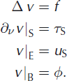
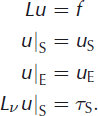
We assume that velocities u S and u E have been prescribed on S and E respectively, that shear stresses τ S have been prescribed on S and that the forcing term f is prescribed in the interior. We wish to find a solution of a regularized Glen flow-law fluid in Ω that satisfies the prescribed boundary conditions. That is, we wish to find a solution to Equation (3) with boundary conditions
where ∇ v is the surface-normal gradient.
This type of boundary-value problem which provides both Dirichlet and Neumann data on part of the boundary and no data on another part is known as a Cauchy problem. The governing partial differential equation (PDE) in Equation (3) is an elliptic second-order differential equation; an elliptic Cauchy problem is a fundamental example of what is known as an ill-posed problem (Reference HadamardHadamard, 1923).
For general data (f, u S, u E, τ S), collectively known as Cauchy data, no solution of this problem exists. Even among data for which a solution exists, the map taking Cauchy data to a solution of Equations (3) and (4) is not continuous in the sense that small perturbations of the data can lead to arbitrarily large effects on the solution. This is the central difficulty presented by ill-posed problems. In practice, one works with a regularization scheme that determines an approximate solution of Equation (3), with the quality of the approximation depending (non-linearly) on the quality of the given Cauchy data. Our approach to finding a regularized solution is based on an iterative method due to Kozlov and Maz’ya for linear Cauchy problems.
For simplicity of discussion, we henceforth assume that τ S, f and u E are known exactly, but u S is subject to measurement error. With regard to τ S, this is not really a restriction since in the physical problem under consideration the surface shear stresses vanish everywhere. Of course, f contains uncertainties (e.g. measurement error in the surface slope and an empirical flow-rate parameter) and u E is an unknown modeled flow. Our method does not treat uncertainties in these terms. Also, measured surface velocities may be affected by features of the flow field that are not captured by our simplified treatment of the Stokes equations, or by the Glen flow law for the full Stokes equations. It would be a mistake to try to fit such features in the data, and we therefore treat inadequacies of our model as errors in u S. If model and data uncertainties can both be described with Gaussian statistics (i.e. are normally distributed), this procedure of adding model uncertainties to the data errors is fully justified (Reference TarantolaTarantola, 2004, p.64). In practice, however, it is often difficult to estimate the model uncertainties.
2.2. Kozlov–Maz’ya iteration for the Laplacian
Reference Kozlov and Maz’yaKozlov and Maz’ya (1990) introduced an iterative scheme for solving the Cauchy problem for the Poisson equation Δu = f; here Δ is the Laplacian, also commonly denoted by ∇ 2. This method has subsequently been extended to general second-order elliptic operators (Reference Kozlov, Maz’ya and FominKozlov and others, 1992), the heat equation (Reference Bastay, Kozlov and TuressonBastay and others, 2001) as well as the linear Stokes equations (Reference Bastay, Johansson, Kozlov and LesnicBastay and others, 2005). We describe the method here first in the context of the Poisson equation. In this case, the Cauchy problem is
To illustrate the ill-posedness of this problem, consider the case of a rectangular domain with x coordinate between 0 and 1 and y coordinate between 0 at the base B and H at the surface S. For the specific data

where k = 1, 2, …, the solution of the Cauchy problem is
Since the value of u at the base y = 0 is sin(kπx) cosh(kH), surface velocities for mode k are amplified at the base by a factor cosh(kπH) which grows exponentially in k. True surface velocities will, of course, not consist of a single high-order mode. However, they can be written in series form ∑ k ak sin(kπx) and (inevitable) errors in measuring the high-order modes will cause uncontrollably large oscillations in the computed basal velocities. The goal of solving the Cauchy problem is to find an approximate solution that does not introduce spurious amplified noise at the base.
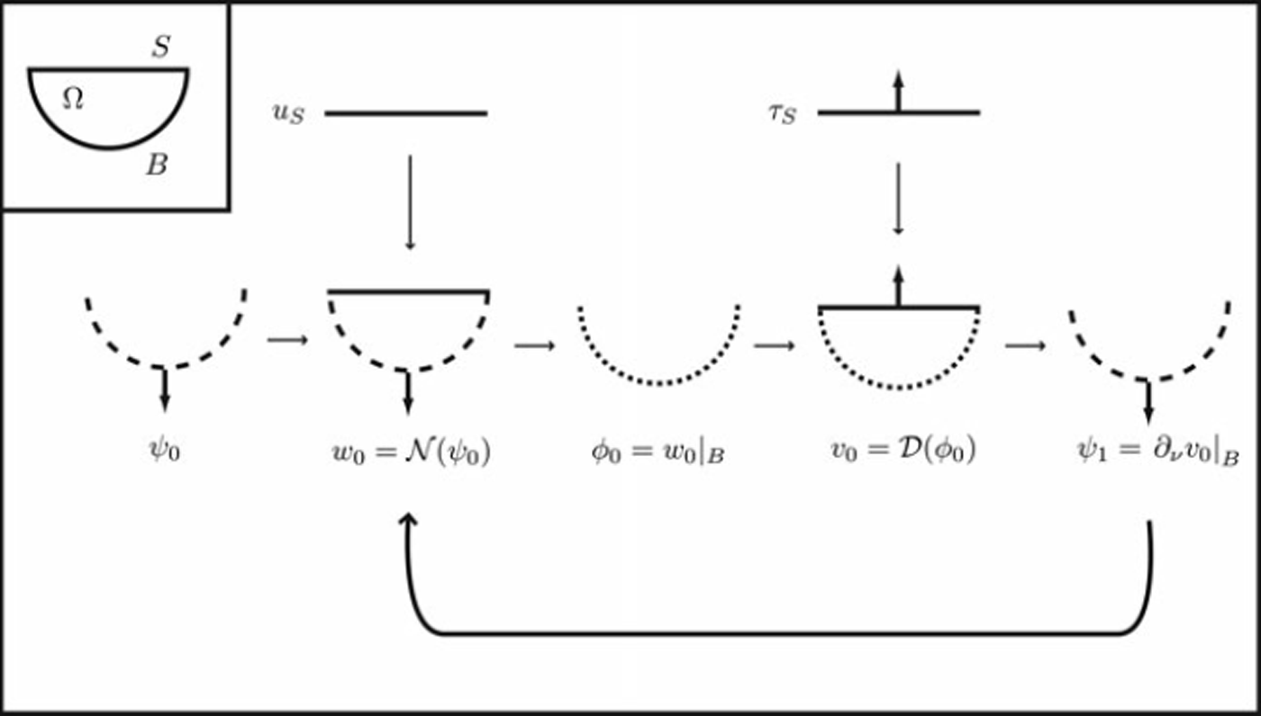
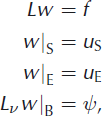
Kozlov–Maz’ya iteration (KM-iteration) uses the two pieces of overdetermined surface data (u S and τ S) in the course of iterating back and forth between a pair of well-posed boundary value problems. The first problem uses the known surface Neumann data τS and a guess for the basal Dirichlet data, ϕ:
The second problem uses the known Dirichlet data uS and a guess for the basal Neumann data ψ:

We let ![]() and
and ![]() be the operators taking ϕ to v and ψ to w, respectively. Note that v and w are down-glacier velocities, not components of a 3-D velocity field.
be the operators taking ϕ to v and ψ to w, respectively. Note that v and w are down-glacier velocities, not components of a 3-D velocity field.
The iterative process now proceeds as follows. Begin with an initial guess ψ
0 for the unknown basal Neumann data and compute ![]() . This provides a guess ϕ
0 for the unknown basal Dirichlet data, namely ϕ
0 = w
0
|
B. We then use this as input into
. This provides a guess ϕ
0 for the unknown basal Dirichlet data, namely ϕ
0 = w
0
|
B. We then use this as input into ![]() to compute
to compute ![]() . Setting ψ
1 = ∂νv
0
|
B, we have now completed one cycle of KM-iteration. This process is outlined schematically in Figure 1.
. Setting ψ
1 = ∂νv
0
|
B, we have now completed one cycle of KM-iteration. This process is outlined schematically in Figure 1.
Flow diagram of Kozlov–Maz’ya iteration. Two well-posed forward problems with different boundary conditions are solved alternately: in the first problem an assumed (or previously calculated) basal shear stress is used together with measured surface velocities. In the second problem, previously calculated basal velocities are used with a zero shear stress assumption at the top boundary. The two problems are solved in iteration until convergence. The dashed line signifies Neumann conditions (basal shear stresses) and the dotted line signifies Dirichlet conditions (velocities).
Let ![]() denote the effect of applying a round of KM-iteration, so
denote the effect of applying a round of KM-iteration, so ![]() . The operator
. The operator ![]() can be thought of as a map from basal shear stresses to basal shear stresses. If a solution u of Equation (5) exists, then ψ = ∂νu|B
is a fixed point of
can be thought of as a map from basal shear stresses to basal shear stresses. If a solution u of Equation (5) exists, then ψ = ∂νu|B
is a fixed point of ![]() . In the notation of Figure 1, if ψ
0 = ∂νu|
B, then w
0 = u, ϕ
0 = u|
B, v
0 = u and ψ
1 = ∂νu|
B. That is,
. In the notation of Figure 1, if ψ
0 = ∂νu|
B, then w
0 = u, ϕ
0 = u|
B, v
0 = u and ψ
1 = ∂νu|
B. That is, ![]() . It was proved by Reference Kozlov and Maz’yaKozlov and Maz’ya (1990) that this fixed point is unique and that the iterates ψk
converge (in a certain sense) to this fixed point. If we start with exact Cauchy data (f, u
S, u
E, τ
S), the iterates ψk
will therefore converge to the exact basal Neumann data ψ. The solution of the Cauchy problem is obtained by finding the unique fixed point of
. It was proved by Reference Kozlov and Maz’yaKozlov and Maz’ya (1990) that this fixed point is unique and that the iterates ψk
converge (in a certain sense) to this fixed point. If we start with exact Cauchy data (f, u
S, u
E, τ
S), the iterates ψk
will therefore converge to the exact basal Neumann data ψ. The solution of the Cauchy problem is obtained by finding the unique fixed point of ![]() .
.
Since the Cauchy data are never known exactly, to obtain a regularized solution we must stop the iterations early. To understand the effect of stopping iterations early, consider again a rectangular domain with x coordinate between 0 and 1 and y coordinate between 0 and H and with all input data set to zero:

The solution of this Cauchy problem is u = 0, and we can observe explicitly howan initial guess for the basal Neumann data ψ 0 converges to zero in this case. (An analysis for the case of non-zero data can be handled by considering the error ψn − ψ between the iterates ψn and the true basal shear stresses ψ.)
Expressing the initial guess ψ0 as a Fourier series
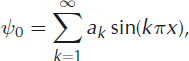
we can apply KM-iteration (which is a linear map in the case of zero data) to each term individually. Supposing that the basal shear stress distribution is of the form of a single-term Fourier series, ψ 0 = sin(kπx), then one round of KM-iteration yields a new guess
where λ k = tanh(kπH). This can be seen by noting that the solution of Equation (9) with ψ = sin(kπx) is
The corresponding basal-velocity distribution is obtained by setting y = 0:
Using this basal-velocity distribution as input in Equation (8) yields a solution
which has a basal shear stress distribution (formed by computing −∂yv at y = 0):
This is the result of a single round of KM-iteration applied to ψ 0. For a full Fourier series, the result of applying m rounds of KM-iteration to ψ 0 is
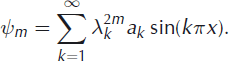
Since each λ k satisfies 0 < λ k < 1, we see that each term in the sum converges to zero. However, the factors λ k converge exponentially to 1, so corrections in the high-order modes occur more and more slowly. This increasing slowness is a desired feature of KM-iteration. The ill-posedness of the Cauchy problem arises from instability in the higher modes (i.e. larger values of k), and KM-iteration performs fast correction on low-order modes while leaving high-order modes nearly unchanged (unless a large number of iterations are performed).
The process of stopping KM-iteration early corresponds to correcting only a collection of low-order modes, starting from an initial guess which expresses an a priori hypothesis concerning the solution (e.g. the glacier is frozen to the bed). For the ill-posed Cauchy problem, we must stop the iterations before they converge, i.e. before we correct modes that our measurement error does not justify correcting. Thus, to be a regularization scheme, KM-iteration must be accompanied by a stopping criterion. Since KM-iteration does not correct errors in the high-order modes of the initial guess, the final result of KM-iteration depends both on the initial guess and the stopping criterion.
One common stopping criterion for iterative inverse methods is the Morozov discrepancy principle (Reference NemirovskiiNemirovskii, 1986; Reference HankeHanke, 1995). In the case of KM-iteration which attempts to solve the fixed point equation ![]() , the discrepancy principle states that we should stop iterations when the fixed point error
, the discrepancy principle states that we should stop iterations when the fixed point error ![]() is smaller than a certain predetermined threshold that expresses our confidence in the Cauchy data. In practice, this threshold is difficult to estimate, and we use an alternative principle described in section 2.5 below.
is smaller than a certain predetermined threshold that expresses our confidence in the Cauchy data. In practice, this threshold is difficult to estimate, and we use an alternative principle described in section 2.5 below.
2.3. Kozlov–Maz’ya iteration for the linearized problem
The method we have described for the Laplacian generalizes to general linear second-order elliptic operators (Reference Kozlov, Maz’ya and FominKozlov and others, 1992). If, for example, L is a second-order elliptic operator of the form
then its corresponding Neumann boundary operator is
and the Cauchy problem for this operator is
The analogues of Equations (8) and (9) are

and
respectively. Just as for the Laplacian, these give rise to operators ![]() and
and ![]() .
.
2.4. Accelerated Kozlov–Maz’ya iteration
Although KM-iteration is a regularization scheme for the Cauchy problem Equation (20), the iterates for this scheme converge quite slowly. Recall that for the rectangular domain with zero initial data (Equation (10)) and a starting guess ![]() , the result of m rounds of KM-iteration is
, the result of m rounds of KM-iteration is

where λ k = tanh(kπH). In order to correct mode k = 4 in a fairly shallow domain with H = 1/3 we have λ4 ∼ 0.9995, and hence more than 2500 iterations are required to reduce the error in this mode to less than 10% of its starting value. While this might be reasonable for a single linear problem, we have found this slowness to be unacceptable as part of an iteration scheme for a non-linear problem.
The slowness of KM-iteration has been addressed by acceleration schemes involving certain tunable relaxation parameters (Reference Jourhmane and NachaouiJourhmane and Nachaoui, 1999; Reference Mera, Elliott, Ingham and LesnicMera and others, 2000). We have developed a general acceleration technique for KM-iteration, based on recasting KM-iteration as a form of a (decelerated) steepest descent scheme for minimizing a certain functional. Using a superior minimization scheme for this functional (the conjugate gradient method) we obtain sufficient acceleration to make KM-iteration feasible as the linear step of a non-linear iteration loop. The Appendix contains a summary of the acceleration scheme; a more complete analysis will be presented in the mathematics literature (D. Maxwell and others, unpublished information).
2.5. Stopping criterion
As mentioned previously, iterative regularization methods require a stopping criterion to ensure that they do not overfit measurement noise. For KM-iteration, which attempts to solve the fixed point problem
an appropriate stopping criterion is that the norm of ![]() be sufficiently small in a certain Sobolev space. A Sobolev space is a vector space of functions equipped with a norm that also includes the derivatives of the functions; they arise naturally in the theory of partial differential equations (Reference Adams and FournierAdams and Fournier, 2003). It can be shown that the level of smallness can be determined by an estimate for the size of the error in the Cauchy data (u
S, τ
S) along with an estimate, specific to the domain geometry, of how surface effects are attenuated at the base. See, for example, the discussion by Reference Bastay, Johansson, Kozlov and LesnicBastay and others (2005).
be sufficiently small in a certain Sobolev space. A Sobolev space is a vector space of functions equipped with a norm that also includes the derivatives of the functions; they arise naturally in the theory of partial differential equations (Reference Adams and FournierAdams and Fournier, 2003). It can be shown that the level of smallness can be determined by an estimate for the size of the error in the Cauchy data (u
S, τ
S) along with an estimate, specific to the domain geometry, of how surface effects are attenuated at the base. See, for example, the discussion by Reference Bastay, Johansson, Kozlov and LesnicBastay and others (2005).
This stopping criterion, however, is difficult to implement in practice since it requires an estimate of geometry-dependent attenuation factors. We have therefore used a heuristic variation of the stopping criterion based on matching the surface Dirichlet condition. Recall that in the course of iterations, vk is a solution of the PDE that matches the surface Neumann data exactly but might not match the surface Dirichlet data well. Given an error threshold δ, we stop iterations at the first k(δ) such that
That is, we stop iterations when vk (δ) approximates (in a root-mean-square sense) u S to within tolerance δ. Although this stopping criterion has worked well for us in practice, we do not have a proof that this is a regularization scheme for KM-iteration.
2.6. Non-linear iterations
The steps of KM-iteration generalize easily to the non-linear Cauchy problem (Equations (3) and (4)). Let ![]() ,
, ![]() and
and ![]() be the non-linear analogs of the operators
be the non-linear analogs of the operators ![]() ,
, ![]() and
and ![]() introduced previously. We wish to solve the fixed-point equation
introduced previously. We wish to solve the fixed-point equation ![]() . Starting with an estimate ψk
for basal shear stresses, let
. Starting with an estimate ψk
for basal shear stresses, let ![]() ,
, ![]() and
and ![]() .
.
It seems reasonable to expect that this iteration method, together with a stopping criterion, would provide a regularization of the non-linear Cauchy problem. A proof of this does not currently exist, however. More importantly, the slowness that presents itself in the linear case is more significant now, because many non-linear boundary value problems need to be solved in the course of the iterations. Moreover, it is not obvious how to directly apply our acceleration scheme from the linear case to the non-linear case. Instead, we have chosen to iterate the linear Cauchy problems in succession.
Suppose u solves

so u satisfies all the requirements of being a solution of the Cauchy problem except for the surface Neumann condition (every output of ![]() satisfies this condition). Let L be the linearization of the non-linear partial differential operator in Equation (3) about u, so
satisfies this condition). Let L be the linearization of the non-linear partial differential operator in Equation (3) about u, so
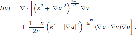
If h is a solution of the linear Cauchy problem
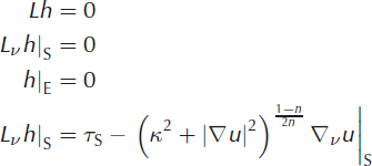
then w = u + h is an approximate solution of the nonlinear Cauchy problem. This suggests an iterative technique for solving the non-linear problem.
Starting with an estimate ψk
−1 for the basal shear stresses, we compute ![]() and
and ![]() . Let
. Let
so ηk is a measure of how close ψk− 1 is to being the solution we seek. For the final solution we would like ηk ≤ δ, but not much smaller. We set Δ k = ηk − δ, so Δ k is the excess error at step k, i.e. the error above the level of desired misfit δ. To compute ψk , we compute the linearized operator Lk corresponding to wk , and perform linear KM-iterations for the linearized Cauchy problem Equation (28) with L = Lk , u = wk and with stopping threshold δk described below. Letting hk be the basal shear stresses resulting from the linear KM-iterations, we set
where λ ∊ [0,1] is obtained by a line search to minimize the error ηk +1. These non-linear iterations stop when ηk < δ.
It is inefficient to use δ as the stopping threshold for early iterations. If wk is far from its final value (which can be detected from the excess error Δ k ), Lk is a comparatively poor approximation for the final non-linear PDE and using the final value of δ results in linear iterations being wasted in finding a very good solution of the Cauchy problem for the wrong operator. Instead, we lower the stopping threshold δk progressively by the rule
where 0 < β < 1 and 0 < μ < 1 are fixed parameters. That is, we attempt to remove 100 (1 − μ)% of the excess error Δ k in the course of solving the linearized Cauchy problem unless the excess error represents less than 100 β% of the error threshold δ, in which case we attempt to remove all excess error. In our computations we used η = 1/2 and β = 1/10.
2.7. Dirichlet starting data
The algorithm, as we have presented it, is a map from basal stresses to basal stresses. Mathematically, KM-iteration is easiest to analyze when thought of this way. This has a practical consequence for our acceleration scheme, which is most simply written when considered as a map from Neumann data to Neumann data. However, it is often desirable to specify an initial guess of Dirichlet data at the base (e.g. a frozen bed). Moreover, it is important to start with a reasonable initial guess – the algorithm is run to convergence only up to a stopping criterion, and the final results depend on the initial guess (refer to the end of section 2.2). It is easy to incorporate an initial guess of Dirichlet data by pre-pending the algorithm with a half KM-iteration (i.e. operator ![]() ).
).
The final output of our algorithm is the output of operator ![]() , and hence satisfies the surface Dirichlet condition exactly but the zero stress condition only approximately. Since we have greater confidence in the surface stress condition, we post-pend a half KM-iteration (operator
, and hence satisfies the surface Dirichlet condition exactly but the zero stress condition only approximately. Since we have greater confidence in the surface stress condition, we post-pend a half KM-iteration (operator ![]() ) to the algorithm. In practice, then, our algorithm can be seen as a map from basal Dirichlet data to Dirichlet data, with inner loops that are maps on Neumann data.
) to the algorithm. In practice, then, our algorithm can be seen as a map from basal Dirichlet data to Dirichlet data, with inner loops that are maps on Neumann data.
2.8. The forward model
The implementation of our method requires the repeated solving of four kinds of forward problems, namely those described by ![]() and
and ![]() (which differ only in their boundary conditions) and their linearized variants
(which differ only in their boundary conditions) and their linearized variants ![]() and
and ![]() . In all cases, we solve the forward problems using the finite-element method. Reference Colinge and RappazColinge and Rappaz (1999) derived the weak form of the non-linear PDE Equation (3), which was then integrated over triangular elements using a given viscosity distribution and linear shape function following standard methods (e.g. Reference ReddyReddy, 2008). To treat the non-linearity in operators
. In all cases, we solve the forward problems using the finite-element method. Reference Colinge and RappazColinge and Rappaz (1999) derived the weak form of the non-linear PDE Equation (3), which was then integrated over triangular elements using a given viscosity distribution and linear shape function following standard methods (e.g. Reference ReddyReddy, 2008). To treat the non-linearity in operators ![]() and
and ![]() , we use the resulting velocity solution to calculate a new viscosity distribution and iterate to convergence. The triangular mesh was generated with the freely available Matlab code distmesh (Reference Persson and StrangPersson and Strang, 2004; http://www-math.mit.edu/∼persson/mesh/). The method was implemented in Matlab and we checked it for convergence with grid refinement.
, we use the resulting velocity solution to calculate a new viscosity distribution and iterate to convergence. The triangular mesh was generated with the freely available Matlab code distmesh (Reference Persson and StrangPersson and Strang, 2004; http://www-math.mit.edu/∼persson/mesh/). The method was implemented in Matlab and we checked it for convergence with grid refinement.
3. Results
We present two sets of results. In the first set, we solve the forward problem with specified bottom boundary conditions. We then, after perturbing the surface velocities with noise, solve the inverse problem to compute basal velocities and compare these computed velocities with the originally prescribed basal boundary condition. In a second set of experiments, we apply the method to actual glaciers (in one case to a glacier with a measured velocity distribution).
3.1. Synthetic data
The performance of any algorithm for constructing regularized solutions of an ill-posed problem depends crucially on the parameters of the associated well-posed problem (i.e. the domain geometry and empirical constants appearing in the PDE). For unfavorable domains, the recovered solution will lack detail and convey little information about the true solution. In order to address the applicability of our inverse method to typical glacier geometries, we considered a sequence of parabolic glacier cross-sections with unit depth and with width 2W; 1 < W < 4. For each cross-section of half-width W, we solved forward problems for Equation (3) (which has units of length−1 time−1/n , so by a suitable choice of timescale any constant forcing term can be rescaled to unity). The solution was found by specifying a constant forcing term f = 1 and basal velocities given by a Gaussian profile

where σ = 1/4, v 0 is half the maximum surface velocity of the solution for the corresponding domain with a frozen base and x = 0 is the center line of the glacier. This provides a localized feature scaled relative to the glacier geometry and typical surface velocity. We then perturbed the computed surface velocities with white noise having amplitude 2% of v 0, and used the perturbed data as input to the inverse method. Figure 2 shows the reconstructed and actual basal velocities.
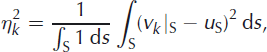
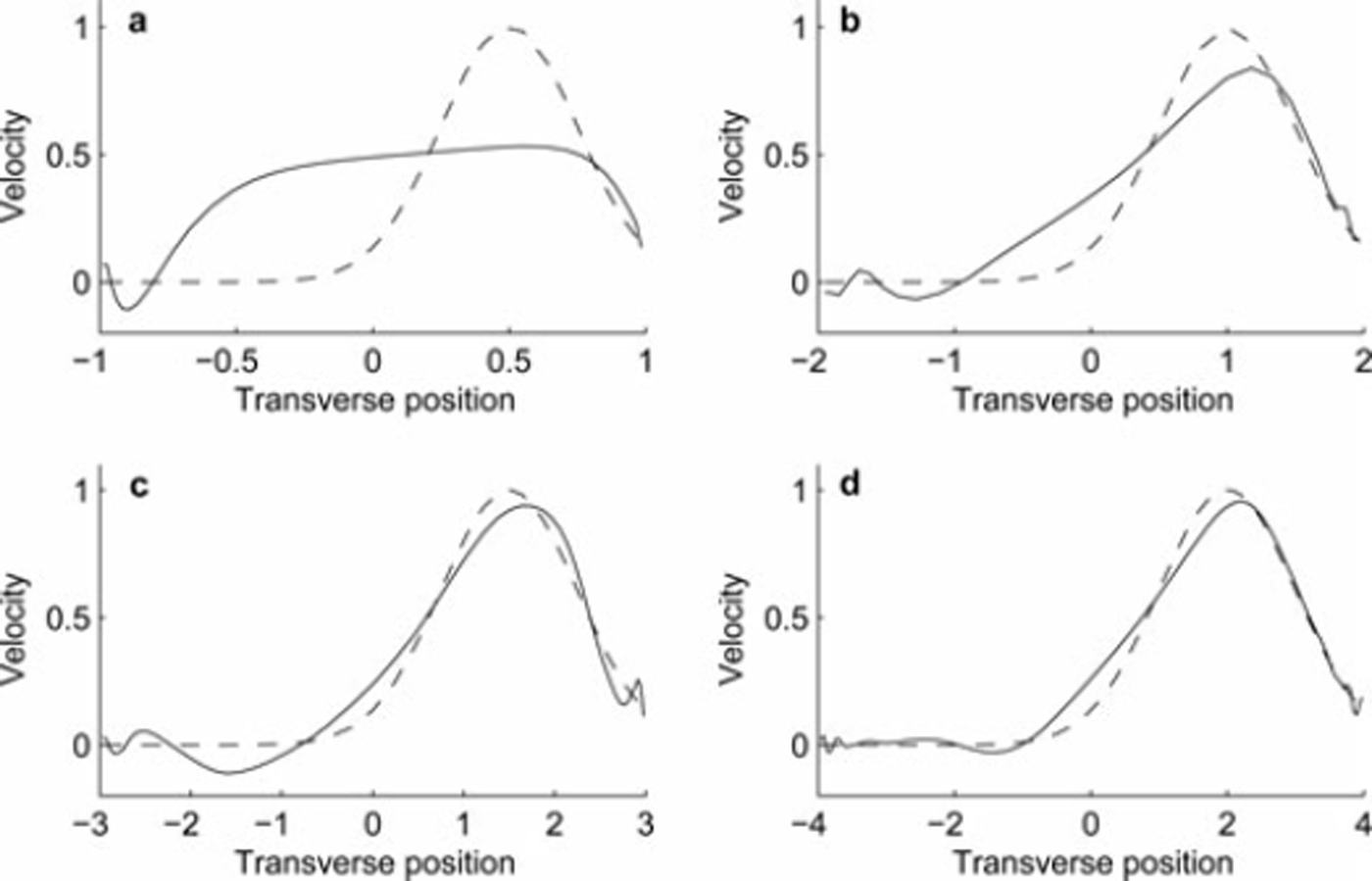
Reconstructed basal velocities for W = (a) 1; (b) 2; (c) 3; and (d) 4. Distances are dimensionless and velocities are rescaled to a common maximum for comparison. Dashed curves show the basal velocity (centered Gaussian distribution) used in the forward model to generate synthetic data, and solid curves are the solutions to the inverse problem.
For W ≥ 2 the algorithm correctly detects significant basal sliding occurring in a region near the center of the glacier, although at W = 2 the peak velocity is somewhat off-center. At W = 1 we are unable to resolve the localized feature and the algorithm constructs a nearly constant basal velocity. In general, increasing W increases both the localization of the velocity peak and the correct recovery of its magnitude.
We used a noise level of 2% in our synthetic tests since this level worked well in reconstructing solutions for real datasets. It is instructive to see the effects of various noise levels on solution quality. Figure 3 shows reconstructions for a domain with W = 2 and noise levels 0.05%, 2% (which corresponds with Fig. 2b), 5% and 10%. We used the same Gaussian basal sliding profile as in Figure 2 for this test. Increasing noise leads to a less defined peak in the reconstruction with a broadening of the sliding region, although even at 0.05% noise there was about 20% error in the peak basal velocity. It is interesting to note that although the predicted peak basal velocity was generally a decreasing function of noise level, this trend did not persist at the 10% noise level where very few iterations were required to match a solution to within the larger error level.
Reconstructed basal velocities from noisy surface velocities for the W = 2 domain. Surface velocities were perturbed with white noise having amplitude (a) 0.5%; (b) 2%; (c) 5%; and (d) 10% of the maximum surface velocity of the solution for this domain of a glacier frozen at the base. Dashed curves show the basal velocity (centered Gaussian distribution) used in the forward model to generate synthetic data, and solid curves are the solutions to the inverse problem.
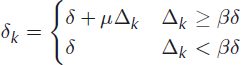
As a further test of resolution, we conducted a similar experiment with Gaussian basal velocity profiles centered at a point halfway between the center and margin (Fig. 4).
Reconstructed basal velocities for W = (a) 1; (b) 2; (c) 3; and (d) 4. Distances are dimensionless and velocities are rescaled to a common maximum for comparison. Dashed curves show the basal velocities (Gaussian distribution centered on three-quarters of the glacier width) used in the forward model to generate synthetic surface data. Solid curves are the solutions of the inverse problem.
Since the velocity peak is located at a lesser depth than the previous experiment, and since there is a non-zero surface velocity at one edge, this is an easier test case than the centered sliding. For W ≥ 2, the algorithm correctly detects localized sliding near the midpoint between the glacier center and edge, with a bias to placing the peak sliding closer to the edge. For W = 1, the algorithm detects that the peak basal velocity occurs to the right, but the solution remains nearly constant over much of the base. Again, increasing W improves the quality of the reconstructed velocity.
Precise velocity features along the base are lost away from the boundary. It is therefore possible that much of the solution in the interior can be reconstructed even when resolution of basal velocities is impossible. Figure 5 shows a comparison of true and reconstructed interior velocities for W = 1 and offset basal sliding. There is good agreement in the interior away from a narrow boundary layer.
(a) True and (b) reconstructed longitudinal velocities for W = 1 with offset basal sliding (Fig. 4a). Units are dimensionless.
Specification of basal velocities together with a zero shear stress condition at the surface determines a unique solution for Equation (3). In principle, all properties of the solution can therefore be determined if the basal velocities can be recovered. We are particularly interested in the shear stresses at the base (which also uniquely determine a solution up to a constant). In practice, however, we expect that the degree to which we can recover shear stresses will be less than that for velocities, since a derivative is required to determine stresses. In order to test the capability of the algorithm to construct shear stresses, we considered for the forward model a Coulomb boundary condition considered by Reference SchoofSchoof (2006). Each point of the base is assumed to have a yield stress τc , and the boundary condition then reads

where n is the flow-law exponent.
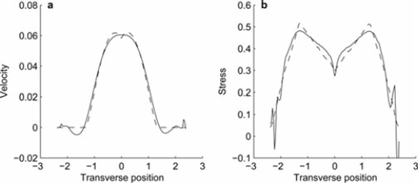
We constructed a forward solution corresponding to figure 4b of Reference SchoofSchoof (2006), where the domain consists of a triangle with unit height and half-width cot(π/8) ∼ 2.4. The yield stress is proportional to overburden pressure up to the water table at height y = 0.84 and is proportional to the difference between overburden and hydrostatic water pressure below the water table. As with the parabolic synthetic data, we added noise to this solution and used the results as input for the inverse method.
Figure 6 shows a comparison of the reconstructed basal velocities and shear stresses. The ice is sliding in a zone of nearly half the glacier width at the base; the shear stress in this region is the yield stress which decreases linearly with depth. The reconstructed solution accurately detects the linear profile and the location of the point where transition to yield stress occurs. There are spurious oscillations in the shear stress near the margin that correlate with oscillations in the reconstructed basal velocities. This is a Gibbs-type phenomenon. A basal velocity that is identically zero in one region and non-zero in another must inherently contain high frequencies, and these will not be resolved by the inverse method.
Comparison of (a) reconstructed basal velocities and (b) basal shear stresses for a Coulomb boundary condition. Units are dimensionless. Dashed curves show the solutions of the forward model and solid curves are the solutions of the inverse problem.
3.2. Real data
3.2.1. Athabasca Glacier
Reference RaymondRaymond (1971) derived velocities along a cross-section of Athabasca Glacier, Canada, by measuring surface velocities and ice deformation in boreholes drilled to the glacier bed. We used the bed geometry and observed surface velocities from this experiment to recover longitudinal velocities in the interior. Our algorithm requires an error threshold for matching the surface velocities; we set this threshold to 2% of the maximum surface velocity.
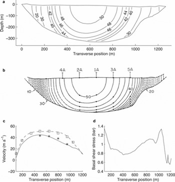
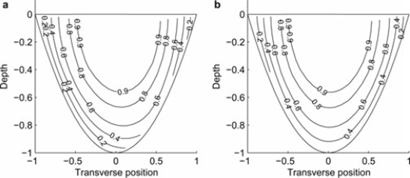
So far we have implicitly assumed that the flow-rate factor A in the constitutive relationship for ice is well known. This is not necessarily the case, and published values vary by almost an order of magnitude (for a review of some published values, see Reference Truffer, Echelmeyer and HarrisonTruffer and others, 2001). On Black Rapids Glacier, Alaska, they found that a value of A = 0.1 bar−3 a−1 worked well. However, using this value we computed longitudinal velocities at the bed of Athabasca Glacier that are approximately 15 m a−1 slower than observed values. This discrepancy is not due to a failure of the inverse method: using the observed bed velocities as input to the forward model yields surface velocities that are significantly faster than observed values. That is, the measured values are incompatible with a Glen flow law with n = 3 and A = 0.1 bar−3 a−1. We obtain significantly better agreement between observed velocities and the velocities obtained by our inverse method by using a stiffer model for ice, in this case with A = 0.063 bar−3 a−1 (Fig. 7).
Athabasca Glacier: (a) modeled velocity contour lines (m a−1); (b) contour lines derived from measurements (Reference RaymondRaymond, 1971); (c) measured (squares) and modeled (dashed curve) surface velocities and measurement-derived (asterisks) and modeled basal velocities (solid curve); and (d) modeled basal shear stress.

We can gain a sense of the level of resolution achieved by considering the eigenmodes (described below) of the linearized Kozlov–Maz’ya iteration operator. Let L be the linearization (about the reconstructed solution u) of the nonlinear partial differential operator in Equation (3), and let ![]() be the corresponding Kozlov–Maz’ya iteration operator with all data (f, u
S, u
E, τ
S) set to zero. For this visualization, it is most convenient to use the Dirichlet-to-Dirichlet operator described in section 2.7.
be the corresponding Kozlov–Maz’ya iteration operator with all data (f, u
S, u
E, τ
S) set to zero. For this visualization, it is most convenient to use the Dirichlet-to-Dirichlet operator described in section 2.7.
A basal-velocity distribution ϕ that satisfies ![]() for some number μ is called an eigenmode of
for some number μ is called an eigenmode of ![]() , and μ is its corresponding eigenvalue. The eigenvalues of
, and μ is its corresponding eigenvalue. The eigenvalues of ![]() can be listed in order 0 < μ
1
< μ
2
< μ
3
< … < 1, and they converge quickly to 1. Roughly speaking, the process of Kozlov–Maz’ya iteration corrects the error by correcting each eigenmode in turn until the stopping criterion is reached. If ϕk
is an eigenmode of
can be listed in order 0 < μ
1
< μ
2
< μ
3
< … < 1, and they converge quickly to 1. Roughly speaking, the process of Kozlov–Maz’ya iteration corrects the error by correcting each eigenmode in turn until the stopping criterion is reached. If ϕk
is an eigenmode of ![]() with eigenvalue μk
, then a perturbation of basal velocities in the direction ϕk
results in a signal at the surface that is approximately attenuated by the factor
with eigenvalue μk
, then a perturbation of basal velocities in the direction ϕk
results in a signal at the surface that is approximately attenuated by the factor ![]() . If V is a characteristic velocity, and if our stopping criterion is set to threshold θV, we therefore expect to detect a signal of size V from the base only for those modes having
. If V is a characteristic velocity, and if our stopping criterion is set to threshold θV, we therefore expect to detect a signal of size V from the base only for those modes having ![]() .
.
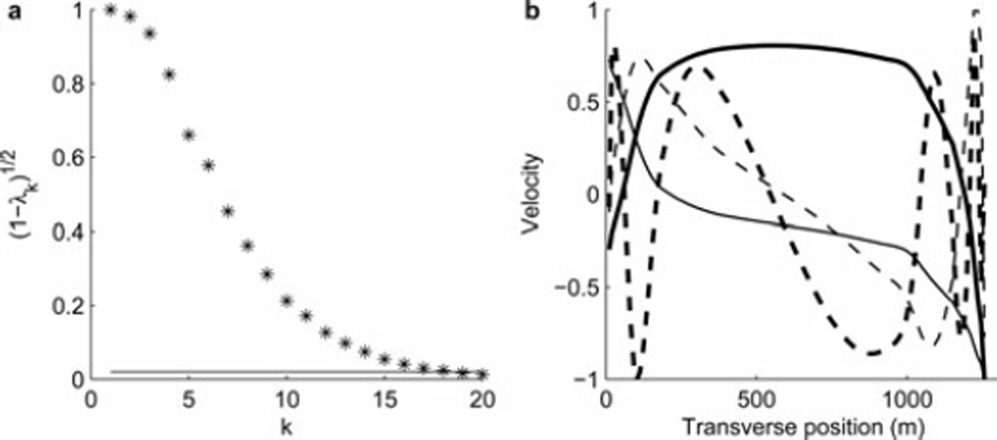
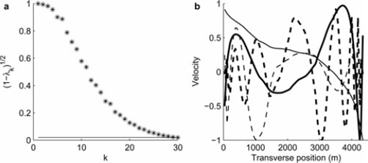
Figure 8 shows the distribution of eigenvalues for the Athabasca Glacier computation, as well as some representative modes. We used a stopping threshold of 2% of the maximum surface velocity; the last value of k with ![]() is k = 18. This mode represents the maximum mode that can be imaged, and only if it were a dominant term in the basal velocity function.
is k = 18. This mode represents the maximum mode that can be imaged, and only if it were a dominant term in the basal velocity function.
(a) Eigenvalues of the Athabasca Kozlov–Maz’ya operator; solid line is the threshold θ = 0.02. (b) Eigenmodes 2 (solid curve), 3 (heavy solid curve), 5 (dashed curve), and 10 (heavy dashed curve). Velocities are dimensionless.
3.2.2. Glaciar Perito Moreno
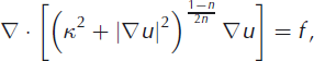
We also applied the method to data from Glaciar Perito Moreno, southern Patagonia icefield. A transverse section of glacier bed topography was derived by seismic methods, and a surface velocity profile was derived from interferometric synthetic aperture radar (InSAR) data (Reference Stuefer, Rott and SkvarcaStuefer and others, 2007). Using the same value of A as for Athabasca Glacier resulted in unphysical basal shear stresses, with the base pulling the ice in places. Using a value of A = 0.1 bar−3 a−1 results in a velocity distribution with significant basal motion along the entire perimeter, but a maximum that is offset from the deepest part of the glacier (Fig. 9).
Glaciar Perito Moreno: (a) contour plot of modeled velocity distribution (m a−1); (b) surface velocities derived from interferometric SAR (squares) and modeled surface (dashed curve) and basal velocities (solid curve); and (c) model-derived basal shear stress.
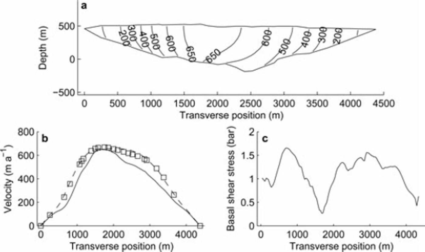
Figure 10 shows the eigenvalue distribution of the ![]() operator and representative modes. We note that the comparative shallowness of Glaciar Perito Moreno manifests itself in a slower decay rate of the eigenvalues. More modes are resolvable than for the Athabasca cross-section, and the resolution is more uniform across the base.
operator and representative modes. We note that the comparative shallowness of Glaciar Perito Moreno manifests itself in a slower decay rate of the eigenvalues. More modes are resolvable than for the Athabasca cross-section, and the resolution is more uniform across the base.
(a) Eigenvalues of the Perito Moreno Kozlov–Maz’ya operator. Solid line is the threshold θ = 0.02. (b) Eigenmodes 2 (solid curve), 6 (heavy solid curve), 10 (dashed curve), and 20 (heavy dashed curve). Velocities are dimensionless.
4. Discussion and Conclusions
We have attempted to resolve basal-velocity distributions from observations that can be made at a glacier surface. There are fundamental limits about the feature size in these derived velocity distributions that can be successfully resolved. Inverse methods can help us determine what these limits are. This aspect of our results is not dependent on the actual method used, although it is possible that the derived velocity fields are.
We have found accelerated KM-iteration to work well and have reasonable convergence properties for our problem. We have experimented with other methods (e.g. Tichonov regularization), but have not found them to perform better.
Numerical experiments with synthetic data show that the recoverability of basal data is strongly dependent on geometry. This can be understood intuitively: a point on the center line of a glacier with half-width to depth ratio of W = 1 is equidistant to its entire perimeter. It is therefore equally sensitive to basal conditions along the entire perimeter. On the other hand, features of the basal velocity field can be better resolved in geometries with higher W. Fortunately, this is the more typical situation in glaciology.
Reference Van der Veen and WhillansVan der Veen and Whillans (1989) proposed a method to calculate englacial velocities by propagating measured velocities downward, using a local force budget. Reference Hantz and LliboutryHantz and Lliboutry (1981), Reference LliboutryLliboutry (1987, ch. 7) and later Reference Bahr, Pfeffer and MeierBahr and others (1994) and Reference LliboutryLliboutry (1995) pointed out the limits of such a scheme and showed that it is not possible to reliably calculate velocities at depths greater than about the half-width of the glacier, due to inherent instabilities.
This can also be seen by observing how small-scale variations in basal boundary conditions propagate upward in a forward (and well-posed) problem (Reference Balise and RaymondBalise and Raymond, 1985). They showed that variations on spatial scales smaller than one ice thickness cannot be resolved by surface measurements. The calculation of transfer functions (Reference Raymond and GudmundssonRaymond and Gudmundsson, 2005) is perhaps the clearest way to illustrate this.
Of course, our method cannot escape such fundamental limits. This is best illustrated by considering Figures 8 and 10: the first few eigenmodes manage to resolve basal velocities near the margins (where the ice is shallow), but only poorly in the deeper parts. In that sense, it is important to point out that our research presents one solution of the inverse problem rather than the solution to the inverse problem (Reference LliboutryLliboutry, 1987, p.180). The result of our iterative method can be intuitively thought of as an approximate solution to the inverse problem obtained by starting with an initial guess and correcting eigenmodes in turn until the resulting solution is compatible (within a prescribed error tolerance) with measured surface data.
Athabasca Glacier is one of only a few glaciers with a dataset suitable for model validation. Our tests with synthetic data indicate that it should be possible to resolve the broad pattern of basal motion, but perhaps not in great detail. As a matter of fact, with a suitable choice of a flow-rate factor, we can reconstruct the measured basal velocities. It should be noted that the measurements are sparse and might also miss smaller-scale variations in the basal-velocity field.
Glacier Perito Moreno has a more favorable geometry (much wider than deep) for basal-velocity reconstruction. Our results indicate large amounts of basal motion along the entire base, with an off-center maximum. The derived stress is minimal near the center of the channel. This is possibly due to low effective pressures (overburden minus water pressures) there. The basal stress distribution looks very similar to that resulting from applying a free boundary problem to failing/non-failing subglacial till, as in Figure 6. A similar stress distribution and off-center velocity maximum was found to reproduce observations on Black Rapids Glacier (Reference Truffer, Echelmeyer and HarrisonTruffer and others, 2001; Reference Amundson, Truffer and LüthiAmundson and others, 2006).
A weakness of the method in its current state is the fact that the constitutive relation for ice is not well enough constrained. Different studies on different glaciers have resulted in proposed values of A for temperate ice that differ by factors of 2 or 3. This discrepancy could be real (due to differences in grain-size distribution or water content), or due to simplifying model assumptions that are being absorbed into model parameters. While some constraints on A result from otherwise unphysical results, it is clear that a rigorous inverse study will also have to solve for a best-fit value for the flow-rate factor A. This might be possible only if ice deformation is measured directly in boreholes.
Another uncertainty is contained in the assessment of the driving stress. Our simplified model assumes a constant outof-plane surface slope, and uncertainties in this slope have a large effect on driving stress and hence ice deformation. Because both the flow-rate factor A and the surface slope occur in the parameter f in Equation (3), the surface slope uncertainty can be absorbed into that of A. This might explain some of the reported variation in A (see section 3.2).
It should be noted that the actual velocity measurement error can be kept very low and, depending on the measurement method, it is not unusual that this error is well below 1%. One should not, however, use this as guidance for the stopping criterion. The reason for this is that there can be features in the velocity field that are not captured by our simple model. It would be a mistake to try to match such features. A practical way of dealing with this issue is to treat the velocities as if they had a larger error. We do not have a rigorous assessment of how large this error should be. We used 2% of maximum surface velocity as the threshold. This seemed to give reasonably detailed basal-velocity fields, but did not show artifacts of overfitting, such as large-amplitude and short-wavelength oscillations. There are also so-called heuristic schemes for determining the stopping threshold, rather than specifying it a priori (Reference HankeHanke, 1995), that would be worth investigating.
Acknowledgements
We thank E. Waddington and an anonymous reviewer for numerous useful suggestions that improved the accessibility of this paper. We also thank our scientific editor, J. Meyssonnier. Research for this work was supported by US National Science Foundation grants OPP 0414128 and ARC 0732602.
Appendix Algorithm for Accelerated KM-Iteration
Let ![]() and
and ![]() be the operators defined by the boundary value problems Equations (8) and (9), respectively.
be the operators defined by the boundary value problems Equations (8) and (9), respectively. ![]() maps basal Dirichlet data to interior velocities using a fixed surface Neumann condition and
maps basal Dirichlet data to interior velocities using a fixed surface Neumann condition and ![]() maps basal Neumann data to interior velocities using a fixed surface Dirichlet condition. For an interior velocity field w, define
maps basal Neumann data to interior velocities using a fixed surface Dirichlet condition. For an interior velocity field w, define ![]() where ψ = ∂νv|B
and v = D(w|B
). Let
where ψ = ∂νv|B
and v = D(w|B
). Let ![]() ,
, ![]() and
and ![]() be the homogeneous versions of these operators (so f, uS
, uE
and τ are all zero in Equations (8) and (9)).
be the homogeneous versions of these operators (so f, uS
, uE
and τ are all zero in Equations (8) and (9)).
Let ψ
0 be an initial guess for the basal Neumann condition and let δ be a stopping tolerance. The following algorithm returns a value of ψ such that ![]() is an approximate solution of the Cauchy problem (Equation (5)).
is an approximate solution of the Cauchy problem (Equation (5)).
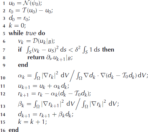
If L is a second-order elliptic differential operator in divergence form, so Lu = ∂i (aij∂ju), then the above algorithm can be applied to the Cauchy problem for L by replacing terms of the form ∫ Ω ∇u ∇v dV ; with the corresponding bilinear form ∫ Ω aij∂iu∂jv dV (and similarly replacing ∫ Ω |∇u|2 dV with ∫ Ω aij∂iu∂ju dV).