1. Introduction
Reliable spectroscopic, photometric, and astrometric data are important for understanding the structure, formation, and evolution of our Galaxy. Today, sky surveys are systematically carried out in a wide range of the electromagnetic spectrum from X-rays to the radio. In some sky surveys such as ROSAT (Snowden Reference Snowden1995), GALEX (Martin et al. Reference Martin2005), and SDSS (York et al. Reference York2000), which are carried out between the X-ray and optical regions of the electromagnetic spectrum, the interstellar absorption prevents to obtain accurate magnitude and colours. However, this problem has been overcame by means of the sky surveys which are defined over the infrared region of the star spectrum, i.e. 2MASS (Skrutskie et al. Reference Skrutskie2006), UKIDSS (Hewett et al. Reference Hewett, Warren, Leggett and Hodgkin1996), VVV (Minniti et al. Reference Minniti2010), VISTA (Cross et al. Reference Cross2012), WISE (Wright et al. Reference Wright2010), and AKARI (Murakami et al. Reference Murakami2007). Thus, considerable information have been obtained, especially on the bulge, bar structure, and Galactic stellar warp in our Galaxy (Dwek et al. Reference Dwek1995; Lopez-Corredoira, Cabrera-Lavers, & Gerhard Reference Lopez-Corredoira, Cabrera-Lavers and Gerhard2005; Lopez-Corredoira et al. Reference Lopez-Corredoira, Lee, Garzon and Lim2019a, b; Benjamin et al. Reference Benjamin2005).
Today, photometric sky survey observations are systematically performed to cover the ultraviolet (UV) and infrared regions of the electromagnetic spectrum. In spectroscopic sky surveys, spectroscopic observations are made for a limited number of objects with different luminosities which are classified according to their positions in colour spaces obtained from the photometric observations. The main sequence stars provide information about the solar neighbourhood, and the evolved stars provide information about the old thin disc, thick disc, and halo populations of our Galaxy beyond the solar vicinity. The number of stars observed on current spectroscopic sky survey programs does not exceed one million in total. As this number is less than needed for a detailed study of the Galactic structure, precise measurements of photometric sky surveys, which contain billions of bright and faint objects, are still important in testing models about the structure and evolution of the Galaxy.
Photometric sky surveys performed in different regions of the electromagnetic spectrum are designed to include shallow or deep magnitudes, according to the purpose of the researchers. However, transformations between different photometric systems can be used as a tool to combine shallow and deep magnitudes. These transformation equations can also be produced in terms of luminosity and metallicity. In the literature, transformation equations are given for main sequence stars (Smith et al. Reference Smith2002; Karaali, Bilir, & Tunçel Reference Karaali, Bilir and Tunçel2005; Bilir, Karaali, & Tunçel Reference Bilir, Karaali and Tunçel2005; Bilir et al. Reference Bilir, Karaali, Ak, Yaz, Cabrera-Lavers and Coşkunoğlu2008a; Bilir et al. Reference Bilir2011; Rodgers et al. Reference Rodgers2006; Jordi et al. Reference Jordi2006; Covey et al. Reference Covey2007; Chonis & Gaskell Reference Chonis and Gaskell2008) and evolved stars (Straizys & Lazauskaite Reference Straizys and Lazauskaite2009; Yaz et al. Reference Yaz2010; Bilir et al. Reference Bilir2012, Reference Bilir, Önal, Karaali, Cabrera-Lavers and Çakmak2013; Ak et al. Reference Ak2014). Transformation equations between the photometric systems have been obtained for approximately 20 years and used effectively to investigate the structure and evolution of our Galaxy.UBV is one of the important photometric system in the optical region (Johnson & Morgan Reference Johnson and Morgan1953) which is used to determine the photometric metallicities of the stars and the interstellar absorption. The  ${U-B}$
colour index plays an important role in these determinations, while its combination with the colour index
${U-B}$
colour index plays an important role in these determinations, while its combination with the colour index  ${B-V}$
can be used in determination of the reddening of stars. In the UBV photometric system, the colour excess
${B-V}$
can be used in determination of the reddening of stars. In the UBV photometric system, the colour excess  ${E(B-V)}$
of a star can be determined by the Q method or by shifting its observed
${E(B-V)}$
of a star can be determined by the Q method or by shifting its observed  ${B-V}$
colour index along the reddening vector in the
${B-V}$
colour index along the reddening vector in the  ${U-B\times B-V}$
two-colour diagram up to the intrinsic colour index
${U-B\times B-V}$
two-colour diagram up to the intrinsic colour index  ${{(B-V)_0}}$
(Johnson & Morgan Reference Johnson and Morgan1953). While the colour excess
${{(B-V)_0}}$
(Johnson & Morgan Reference Johnson and Morgan1953). While the colour excess  ${E(U-B)}$
can be calculated by the equation of the reddening line, i.e.
${E(U-B)}$
can be calculated by the equation of the reddening line, i.e.  ${E(U-B)=0.72\times E(B-V)+0.05\times E(B-V)^2}$
. Roman (Reference Roman1955) discovered that stars with weak metal lines have larger ultraviolet (UV) excesses than the ones with strong metal lines. Schwarzschild, Searle, & Howard (Reference Schwarzschild, Searle and Howard1955), Sandage & Eggen (Reference Sandage and Eggen1959), and Wallerstein (Reference Wallerstein1962) confirmed the work of Roman (Reference Roman1955). Thus, metal-rich and metal-poor stars could be classified not only spectroscopically but also photometrically, i.e. by their UV excesses. Sandage (Reference Sandage1969) noticed in a
${E(U-B)=0.72\times E(B-V)+0.05\times E(B-V)^2}$
. Roman (Reference Roman1955) discovered that stars with weak metal lines have larger ultraviolet (UV) excesses than the ones with strong metal lines. Schwarzschild, Searle, & Howard (Reference Schwarzschild, Searle and Howard1955), Sandage & Eggen (Reference Sandage and Eggen1959), and Wallerstein (Reference Wallerstein1962) confirmed the work of Roman (Reference Roman1955). Thus, metal-rich and metal-poor stars could be classified not only spectroscopically but also photometrically, i.e. by their UV excesses. Sandage (Reference Sandage1969) noticed in a  ${{(U-B)_0\times(B-V)_0}}$
two-colour diagram of a set of stars in solar neighbourhood that stars with the same metallicity have a maximum UV excess at the colour index
${{(U-B)_0\times(B-V)_0}}$
two-colour diagram of a set of stars in solar neighbourhood that stars with the same metallicity have a maximum UV excess at the colour index  ${{(B-V)_0=0.6}}$
mag and introduced a procedure to reduce the UV excesses of the stars to the one of colour index
${{(B-V)_0=0.6}}$
mag and introduced a procedure to reduce the UV excesses of the stars to the one of colour index  ${{(B-V)_0=0.6}}$
mag. The relation between the UV excess and metallicities of stars has been used by the researchers for their metallicity estimation via photometry (i.e. Carney Reference Carney1979; Karaali et al. Reference Karaali, Ak, Bilir, Karataş and Gilmore2003a, b, c; Karataş & Schuster Reference Karataş and Schuster2006; Karaali et al. Reference Karaali, Bilir, Ak, Yaz and Coşkunoğlu2011; Tunçel Güçtekin et al. Reference Tunçel Güçtekin, Bilir, Karaali, Ak, Ak and Bostanc2016; Çelebi et al. Reference Çelebi, Bilir, Ak, Ak, Bostancı and Yontan2019). Similar calibrations have been developed for the SDSS photometric system and applied to faint stars (Karaali et al. Reference Karaali, Bilir and Tunçel2005; Bilir et al. Reference Bilir, Karaali and Tunçel2005; Tunçel Güçtekin et al. Reference Tunçel Güçtekin, Bilir, Karaali, Plevne, Ak, Ak and Bostanci2017). These calibrations were used to calculate metal abundances (Ak et al. Reference Ak, Bilir, Karaali, Buser and Cabrera-Lavers2007; Ivezic et al. Reference Ivezic2008; Tunçel Güçtekin et al. Reference Tunçel Güçtekin, Bilir, Karaali, Plevne and Ak2019) and estimation of the Galactic model parameters for different populations (Karaali, Bilir, & Hamzaoğlu Reference Karaali, Bilir and Hamzaoğlu2004; Ak et al. Reference Ak, Bilir, Karaali, Buser and Cabrera-Lavers2007; Bilir et al. Reference Bilir2008b; Juric et al. Reference Juric2008; Yaz & Karaali Reference Yaz and Karaali2010).
${{(B-V)_0=0.6}}$
mag. The relation between the UV excess and metallicities of stars has been used by the researchers for their metallicity estimation via photometry (i.e. Carney Reference Carney1979; Karaali et al. Reference Karaali, Ak, Bilir, Karataş and Gilmore2003a, b, c; Karataş & Schuster Reference Karataş and Schuster2006; Karaali et al. Reference Karaali, Bilir, Ak, Yaz and Coşkunoğlu2011; Tunçel Güçtekin et al. Reference Tunçel Güçtekin, Bilir, Karaali, Ak, Ak and Bostanc2016; Çelebi et al. Reference Çelebi, Bilir, Ak, Ak, Bostancı and Yontan2019). Similar calibrations have been developed for the SDSS photometric system and applied to faint stars (Karaali et al. Reference Karaali, Bilir and Tunçel2005; Bilir et al. Reference Bilir, Karaali and Tunçel2005; Tunçel Güçtekin et al. Reference Tunçel Güçtekin, Bilir, Karaali, Plevne, Ak, Ak and Bostanci2017). These calibrations were used to calculate metal abundances (Ak et al. Reference Ak, Bilir, Karaali, Buser and Cabrera-Lavers2007; Ivezic et al. Reference Ivezic2008; Tunçel Güçtekin et al. Reference Tunçel Güçtekin, Bilir, Karaali, Plevne and Ak2019) and estimation of the Galactic model parameters for different populations (Karaali, Bilir, & Hamzaoğlu Reference Karaali, Bilir and Hamzaoğlu2004; Ak et al. Reference Ak, Bilir, Karaali, Buser and Cabrera-Lavers2007; Bilir et al. Reference Bilir2008b; Juric et al. Reference Juric2008; Yaz & Karaali Reference Yaz and Karaali2010).
Spectroscopic data used in this study. N denotes the number of stars, R spectral resolution,  ${S/N}$
signal-to-noise ratio. Observatory, telescope, and the spectrograph used in the observations are also noted.
${S/N}$
signal-to-noise ratio. Observatory, telescope, and the spectrograph used in the observations are also noted.
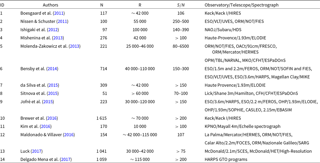
CASLEO: Complejo Astronomico El Leoncito, EBASIM: Echellede Banco Simmons, CFH: Canada-France-Hawaii, CFHT: Canada-France-Hawaii Telescope, ESO: European Southern Observatory, ESPaDOnS: an Echelle SpectroPolarimetric Device for the Observation of Stars at CFHT, FEROS: The Fiber-Fed Extended Range Optical Spectrograph, FIES: The High-Resolution Fibre-Fed Echelle Spectrograph, FOCES: a Fibre Optics Cassegrain Echelle Spectrograph, FRESCO: Fiber-Optic Reosc Echelle Spectrograph of Catania Observatory, GTO: Guaranteed Time Observations, HARPS: High Accuracy Radial Velocity Planet Searcher, HERMES: High-Efficiency and High-Resolution Mercator Echelle Spectrograph, HET: Hobby-Eberly Telescope, HDS: High Dispersion Spectrograph, HIRES: High-Resolution Echelle Spectrometer, KPNO: Kitt Peak National Observatory, MIKE: Magellan Inamori Kyocera Echelle, MKO: Mauna Kea Observatory, NAOJ: National Astronomical Observatory of Japan, NOT: Nordic Optical Telescope, OACt: Catania Astrophysical Observatory, OPM: Observatorie Pic du Midi, ORM: Observatorio del Roque de losMuchachos, SCES: Sandiford Cassegrain Echelle Spectrograph, SOFIN: The Soviet-Finnish Optical High-Resolution Spectrograph, SOPHIE: Spectrographe pour l’Observation des Phenomenes des Interieurs stellaires et des Exoplanetes, TBL: Telescope Bernard Lyot, UVES: Ultraviolet and Visual Echelle Spectrograph, VLT: Very Large Telescope.
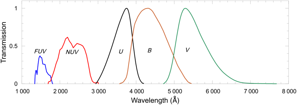
Normalized transmission curves of the GALEX FUV, NUV and Johnson-Morgan U, B, V filters.
The basic parameters of 556 sample stars; ID, star, equatorial coordinates in J2000 ( ${\alpha}$
,
${\alpha}$
,  ${\delta}$
), photometric data (FUV, NUV, V,
${\delta}$
), photometric data (FUV, NUV, V,  ${U-B}$
,
${U-B}$
,  ${B-V}$
), reduced colour excess (
${B-V}$
), reduced colour excess ( ${E_d(B-V)}$
), atmospheric model parameters (
${E_d(B-V)}$
), atmospheric model parameters ( ${T_{\rm eff}}$
,
${T_{\rm eff}}$
,  ${\log g}$
and [Fe/H]) and their references, and trigonometric parallaxes (
${\log g}$
and [Fe/H]) and their references, and trigonometric parallaxes ( ${\pi}$
) with the errors taken from Gaia DR2.
${\pi}$
) with the errors taken from Gaia DR2.
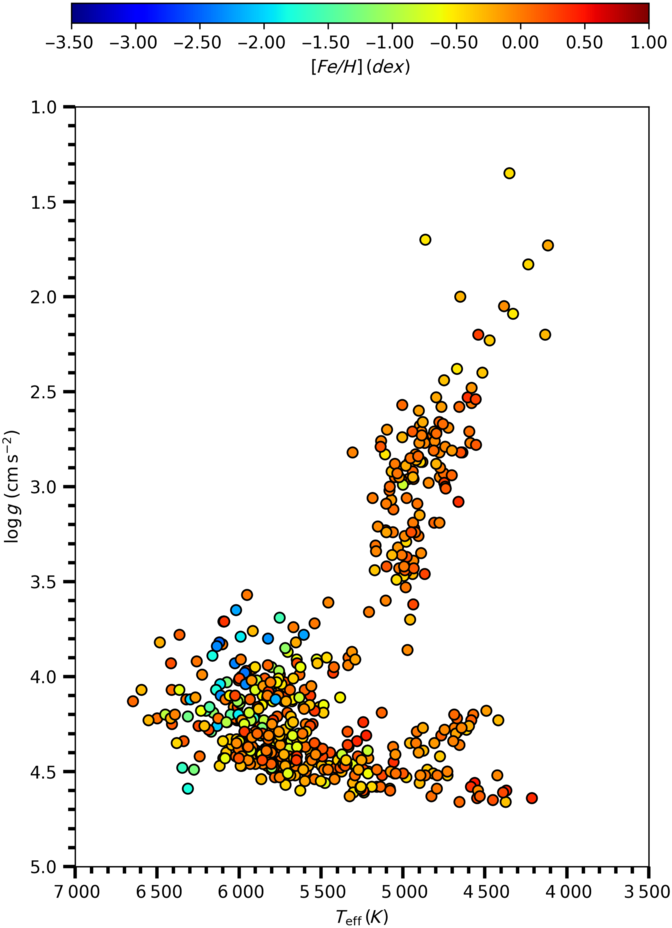
 ${\log g \times T_{\rm eff}}$
diagram of the stars in the sample. The diagram is colour-coded for the metallicity of 556 stars.
${\log g \times T_{\rm eff}}$
diagram of the stars in the sample. The diagram is colour-coded for the metallicity of 556 stars.
The UBV photometric system provides reliable data for the bright stars which occupy the solar neighbourhood. However, for the faint stars the same case thus not hold. Additionally, the low transmission of the Earth’s atmosphere limits the number of stars with reliable U magnitudes. This problem could be solved by measurements performed outside of the atmosphere such as the satellite Galaxy Evolution Discovery (GALEX) (Martin et al. Reference Martin2005).
The GALEX satellite was launched in 2003 and continued its active mission until 2012. It is the first satellite to observe the entire sky with the two detectors, i.e. far ultraviolet (FUV,  ${\lambda_{\rm eff}}$
= 1 528 Å; 1 344–1 786 Å) and near ultraviolet (NUV,
${\lambda_{\rm eff}}$
= 1 528 Å; 1 344–1 786 Å) and near ultraviolet (NUV,  ${\lambda_{\rm eff}}$
= 2 310 Å; 1 771–2 831 Å). The passbands of GALEX and UBV photometric systems are shown in Figure 1. Measurements in the far and near UV bands of approximately 583 million objects obtained from the reduction of 100 865 images from satellite observations are given in DR 6+7 versions of GALEX database (Bianchi, Shiao, & Thilker Reference Bianchi, Shiao and Thilker2017). In our study, transformation equations between the colour indices of GALEX and UBV photometric systems are derived in terms of the luminosity class. These equations provide us empirical
${\lambda_{\rm eff}}$
= 2 310 Å; 1 771–2 831 Å). The passbands of GALEX and UBV photometric systems are shown in Figure 1. Measurements in the far and near UV bands of approximately 583 million objects obtained from the reduction of 100 865 images from satellite observations are given in DR 6+7 versions of GALEX database (Bianchi, Shiao, & Thilker Reference Bianchi, Shiao and Thilker2017). In our study, transformation equations between the colour indices of GALEX and UBV photometric systems are derived in terms of the luminosity class. These equations provide us empirical  ${U-V}$
colour index and UV excess for stars which can be used in photometric metal abundance estimation. We organized the paper as follows. Section 2 is devoted to the selection of the calibration stars in our study, derivation of the calibrations is given in Section 3, and finally, the results and discussion are presented in Section 4.
${U-V}$
colour index and UV excess for stars which can be used in photometric metal abundance estimation. We organized the paper as follows. Section 2 is devoted to the selection of the calibration stars in our study, derivation of the calibrations is given in Section 3, and finally, the results and discussion are presented in Section 4.
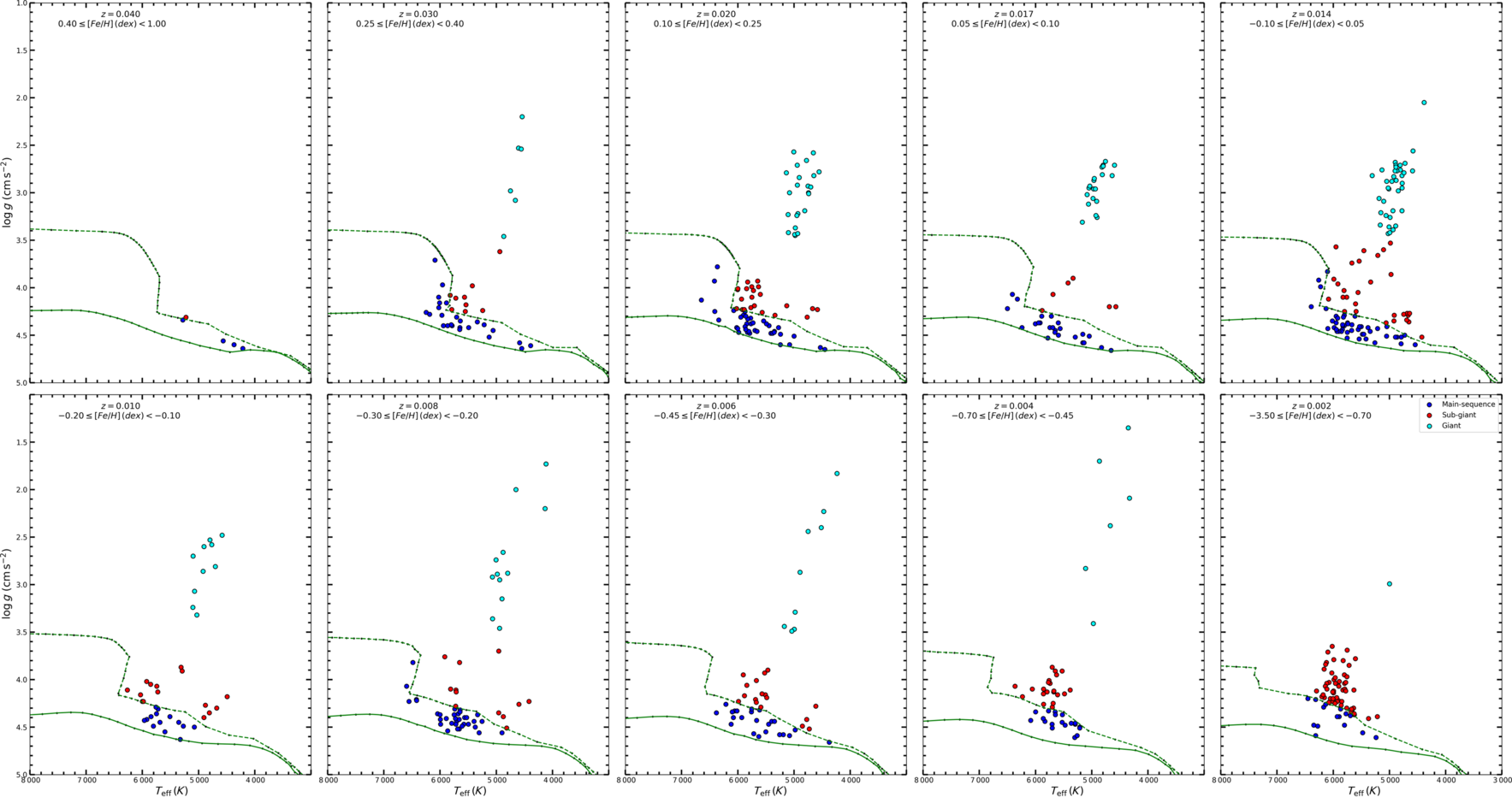
 ${\log g \times T_{\rm eff}}$
diagram of the stars with different metallicity intervals. Blue circle: main sequence, red circle: sub-giants and cyan circle: giant stars. Green solid and dashed curves represent the ZAMS and TAMS, respectively.
${\log g \times T_{\rm eff}}$
diagram of the stars with different metallicity intervals. Blue circle: main sequence, red circle: sub-giants and cyan circle: giant stars. Green solid and dashed curves represent the ZAMS and TAMS, respectively.
2. Data
In this study, we prioritized the stars that have precise spectroscopic, astrometric, and photometric data in the literature. In this context, we used the spectroscopic data from 14 studies (Boesgaard et al. Reference Boesgaard2011; Nissen & Schuster Reference Nissen and Schuster2011; Ishigaki, Chiba, & Aoki Reference Ishigaki, Chiba and Aoki2012; Mishenina et al. Reference Mishenina, Pignatari, Korotin, Soubiran, Charbonnel, Thielemann, Gorbaneva and Basak2013; Molenda-Zakowicz et al. Reference Molenda-Zakowicz2013; Bensby, Feltzing, & Oey Reference Bensby, Feltzing and Oey2014; da Silva, Milone, & Rocha-Pinto, Reference da Silva, Milone and Rocha-Pinto2015; Sitnova et al. Reference Sitnova2015; Jofré et al. Reference Jofré2015; Brewer et al. Reference Brewer, Fischer, Valenti and Piskunov2016; Kim et al. Reference Kim2016; Maldonado & Villaver Reference Maldonado and Villaver2016; Luck Reference Luck2017; Delgado Mena et al. Reference Delgado Mena, Tsantaki, Adibekyan, Sousa, Santos, Gonzalez Hernandez and Israelian2017). Totally, 6 149 stars with atmospheric model parameters ( ${T_{\rm eff}}$
,
${T_{\rm eff}}$
,  ${\log g}$
and [Fe/H]) could be provided from these studies (Table 1). The photometric data are supplied from GALEX DR7 (Bianchi et al. Reference Bianchi, Shiao and Thilker2017) and UBV (Oja Reference Oja1984; Mermilliod Reference Mermilliod1987, Reference Mermilliod1997; Ducati Reference Ducati2002; Koen et al. Reference Koen, Kilkenny, van Wyk and Marang2010; Carrasco et al. Reference Carrasco, Loyola, Moreno and Ledoux2010), while the trigonometric parallaxes are taken from Gaia DR2 (Gaia Collaboration et al. Reference Collaboration2018). The photometric and astrometric data of 5 593 stars were not available for the original set of stars (6 149 stars). Hence, our sample reduced to 556 (Table 2).
${\log g}$
and [Fe/H]) could be provided from these studies (Table 1). The photometric data are supplied from GALEX DR7 (Bianchi et al. Reference Bianchi, Shiao and Thilker2017) and UBV (Oja Reference Oja1984; Mermilliod Reference Mermilliod1987, Reference Mermilliod1997; Ducati Reference Ducati2002; Koen et al. Reference Koen, Kilkenny, van Wyk and Marang2010; Carrasco et al. Reference Carrasco, Loyola, Moreno and Ledoux2010), while the trigonometric parallaxes are taken from Gaia DR2 (Gaia Collaboration et al. Reference Collaboration2018). The photometric and astrometric data of 5 593 stars were not available for the original set of stars (6 149 stars). Hence, our sample reduced to 556 (Table 2).
Distribution of 556 sample stars according to the luminosity classes and the metallicity intervals.
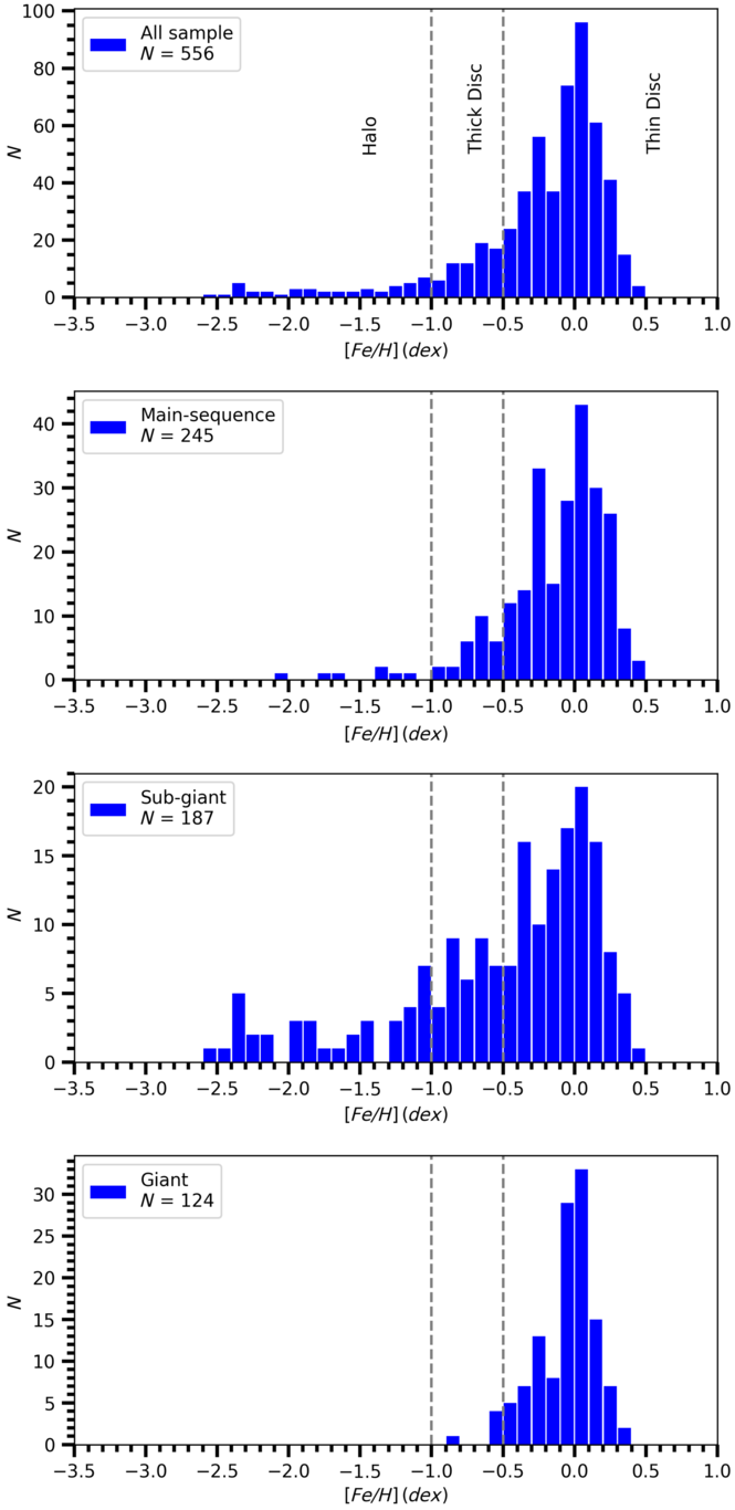
Distribution of the spectroscopic metal abundances for all sample, main sequence, sub-giant, and giant stars.
The  ${\log g \times T_{\rm eff}}$
diagram of the sample stars is shown in Figure 2 with the colour coded for metallicity [Fe/H]. PARSEC mass tracks for different metal abundances are used to determine the luminosity classes of the sample stars (Bressan et al. Reference Bressan2012; Tang et al. Reference Tang2014; Chen et al. Reference Chen, Bressan, Girardi, Marigo, Kong and Lanza2015). The evolutionary tracks generated for different heavy element abundances (Z = 0.040, 0.030, 0.020, 0.017, 0.014, 0.010, 0.008, 0.006, 0.004, and 0.002) are converted to [Fe/H] metallicities using the formulae given by Jo BovyFootnote a
(see also Bostanci et al. Reference Bostancı2018; Eker et al. Reference Eker2018; Yontan et al. Reference Yontan2019; Banks et al. Reference Banks, Yontan, Bilir and Canbay2020). Then, zero age main sequence (ZAMS) and terminal age main sequence (TAMS) evolutionary tracks corresponding to the metal abundance ranges for mean Z values were established (Figure 3). The luminosity classes of the sample stars were determined by the metallicity intervals as indicated in Figure 3 and marked on the
${\log g \times T_{\rm eff}}$
diagram of the sample stars is shown in Figure 2 with the colour coded for metallicity [Fe/H]. PARSEC mass tracks for different metal abundances are used to determine the luminosity classes of the sample stars (Bressan et al. Reference Bressan2012; Tang et al. Reference Tang2014; Chen et al. Reference Chen, Bressan, Girardi, Marigo, Kong and Lanza2015). The evolutionary tracks generated for different heavy element abundances (Z = 0.040, 0.030, 0.020, 0.017, 0.014, 0.010, 0.008, 0.006, 0.004, and 0.002) are converted to [Fe/H] metallicities using the formulae given by Jo BovyFootnote a
(see also Bostanci et al. Reference Bostancı2018; Eker et al. Reference Eker2018; Yontan et al. Reference Yontan2019; Banks et al. Reference Banks, Yontan, Bilir and Canbay2020). Then, zero age main sequence (ZAMS) and terminal age main sequence (TAMS) evolutionary tracks corresponding to the metal abundance ranges for mean Z values were established (Figure 3). The luminosity classes of the sample stars were determined by the metallicity intervals as indicated in Figure 3 and marked on the  ${\log g \times T_{\rm eff}}$
diagrams. Stars between the ZAMS and TAMS curves are classified as main sequence stars, while the ones above the TAMS curve are adopted as evolved stars, i.e. those with
${\log g \times T_{\rm eff}}$
diagrams. Stars between the ZAMS and TAMS curves are classified as main sequence stars, while the ones above the TAMS curve are adopted as evolved stars, i.e. those with  ${\log\ g\geq 3.5}$
as sub-giants and the ones with
${\log\ g\geq 3.5}$
as sub-giants and the ones with  ${\log\ g<3.5}$
as giants. Thus, the number of stars with different luminosity classes turned out to be as follows: 245 main sequence, 187 sub-giants, and 124 giants.
${\log\ g<3.5}$
as giants. Thus, the number of stars with different luminosity classes turned out to be as follows: 245 main sequence, 187 sub-giants, and 124 giants.
We used the atmospheric model parameters to classify the luminosity class of each star. The giant stars tend to be well separated from the sub-giants, while the sub-giants are very close to the main sequence stars. Hence, we investigated the uncertainty of the atmospheric model parameters to reveal any contamination of the sub-giants into the main sequence region and vice versa, as explained in the following. As the uncertainty of the atmospheric model parameters was not considered in some studies which cover our sample stars (556 stars), we used the uncertainty of the atmospheric model parameters in Bensby et al. (Reference Bensby, Feltzing and Oey2014) which contains approximately 22% of the stars in the sample, for our purpose. The median errors of  ${T_{\rm eff}}$
,
${T_{\rm eff}}$
,  ${\log g}$
, and [Fe/H] in Bensby et al. (Reference Bensby, Feltzing and Oey2014) are 56 K,
${\log g}$
, and [Fe/H] in Bensby et al. (Reference Bensby, Feltzing and Oey2014) are 56 K,  ${0.08\text{ cm s}^{-2}}$
, and 0.05 dex, respectively. The luminosity classes of the stars in the sample were determined by comparing the atmospheric model parameters of the stars with the ZAMS and TAMS curves designated from the PARSEC mass tracks. The median errors of the atmospheric model parameters were added to the original parameters of the stars, and their luminosity classes were reassigned. Stars, whose luminosity classes were changed, were considered as contamination. It is found that the contamination of the main sequence stars by sub-giant stars is 2.9%, the contamination of sub-giant stars by main sequence is 3.7%, and the contamination of giant stars by sub-giant stars is 3.2%. Hence, one can say that our transformation equations can be considered for the luminosity class of the sample stars in question.
${0.08\text{ cm s}^{-2}}$
, and 0.05 dex, respectively. The luminosity classes of the stars in the sample were determined by comparing the atmospheric model parameters of the stars with the ZAMS and TAMS curves designated from the PARSEC mass tracks. The median errors of the atmospheric model parameters were added to the original parameters of the stars, and their luminosity classes were reassigned. Stars, whose luminosity classes were changed, were considered as contamination. It is found that the contamination of the main sequence stars by sub-giant stars is 2.9%, the contamination of sub-giant stars by main sequence is 3.7%, and the contamination of giant stars by sub-giant stars is 3.2%. Hence, one can say that our transformation equations can be considered for the luminosity class of the sample stars in question.
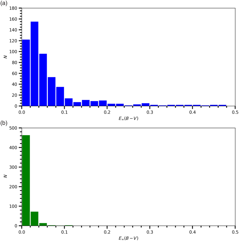
Histograms of the original  ${E_{\infty}(B-V)}$
(a) and reduced
${E_{\infty}(B-V)}$
(a) and reduced  ${E_d(B-V)}$
(b) colour excesses of 556 stars.
${E_d(B-V)}$
(b) colour excesses of 556 stars.
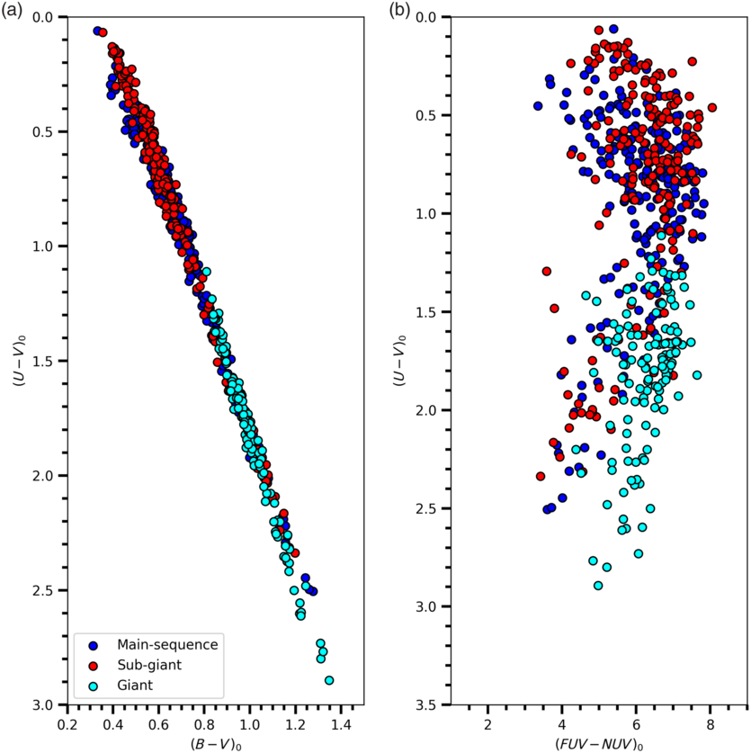
Distribution of the sample stars in the  ${{(U-V)_0\times(B-V)_0}}$
(a) and
${{(U-V)_0\times(B-V)_0}}$
(a) and  ${{(U-V)_0\times(FUV-NUV)_0}}$
(b) two-colour diagrams, colour coded for the luminosity class as indicated.
${{(U-V)_0\times(FUV-NUV)_0}}$
(b) two-colour diagrams, colour coded for the luminosity class as indicated.
Coefficients derived from Equation (4) and the corresponding squared correlation coefficient ( ${R^2}$
) and standard deviation (
${R^2}$
) and standard deviation ( ${\sigma}$
), for the sample stars of different luminosity classes. The metallicities are not considered in these calculations. N indicates the number of stars. The remaining symbols are explained in the text.
${\sigma}$
), for the sample stars of different luminosity classes. The metallicities are not considered in these calculations. N indicates the number of stars. The remaining symbols are explained in the text.

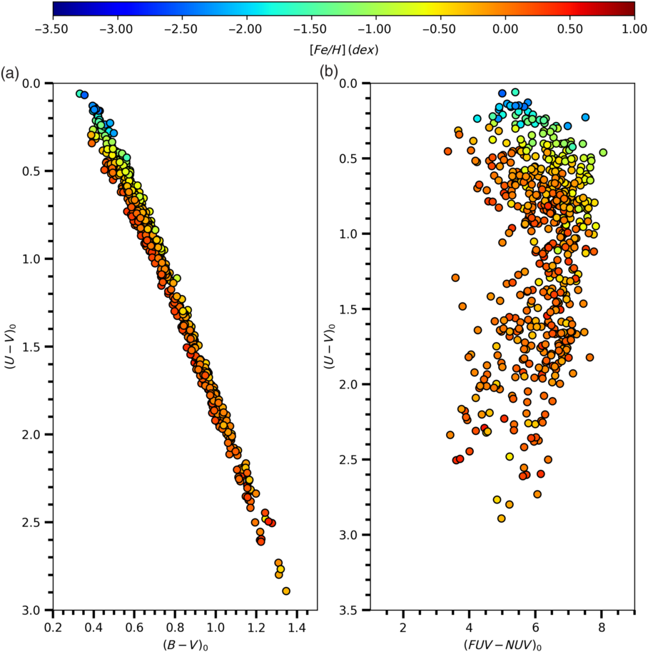
Distribution of the sample stars in the  ${{(U-V)_0\times(B-V)_0}}$
(a) and
${{(U-V)_0\times(B-V)_0}}$
(a) and  ${{(U-V)_0\times(FUV-NUV)_0}}$
(b) two-colour diagrams, colour coded for the metallicity as indicated.
${{(U-V)_0\times(FUV-NUV)_0}}$
(b) two-colour diagrams, colour coded for the metallicity as indicated.
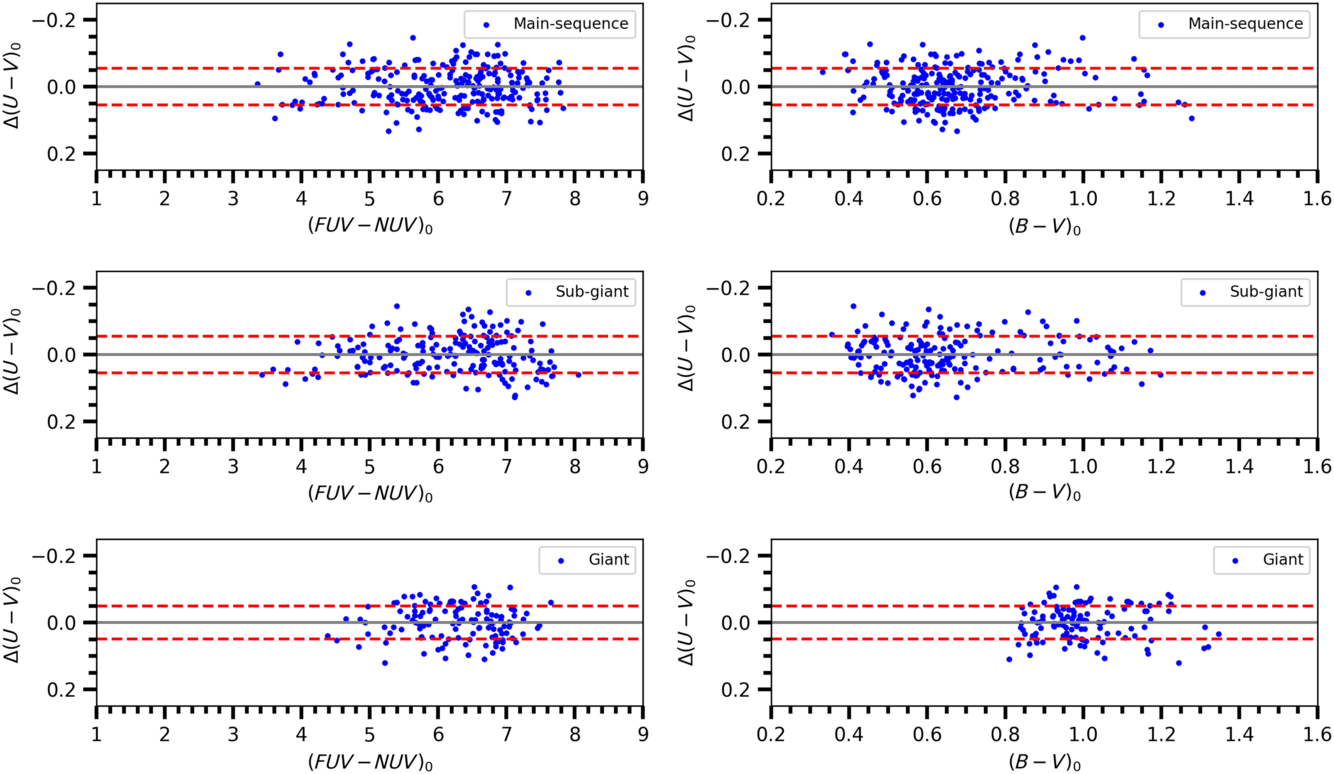
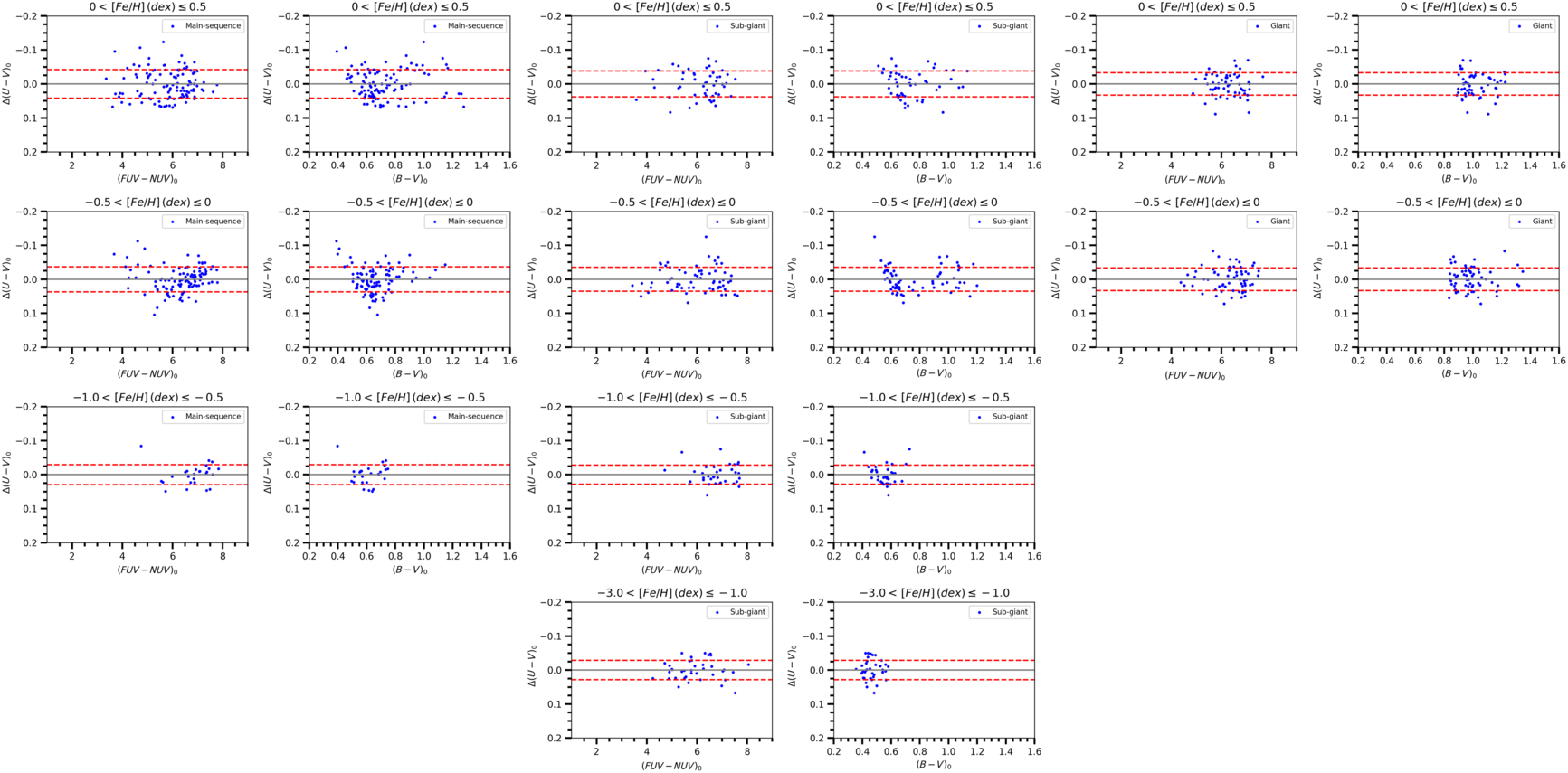
Colour residuals in terms of  ${{(FUV-NUV)_0}}$
(left column) and
${{(FUV-NUV)_0}}$
(left column) and  ${{(B-V)_0}}$
(right column) for three luminosity classes as indicated in six panels. Metallicity is not considered in calculation of the residuals. Dashed lines denote
${{(B-V)_0}}$
(right column) for three luminosity classes as indicated in six panels. Metallicity is not considered in calculation of the residuals. Dashed lines denote  ${\pm 1\sigma}$
prediction levels.
${\pm 1\sigma}$
prediction levels.
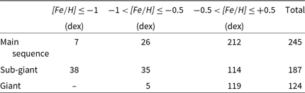
The sample stars were also separated into different population types according to their metallicities, i.e. thin disc ( ${-0.5 <{\rm[Fe/H]}<+0.5\text{ dex}}$
), thick disc (
${-0.5 <{\rm[Fe/H]}<+0.5\text{ dex}}$
), thick disc ( ${-1<{\rm[Fe/H]}<-0.5\text{ dex}}$
), and halo (
${-1<{\rm[Fe/H]}<-0.5\text{ dex}}$
), and halo ( ${{\rm [Fe/H]}<-1\text{ dex}}$
), and they were listed in Table 3. The metallicity distribution for all stars and for different luminosity classes is given in Figure 4.
${{\rm [Fe/H]}<-1\text{ dex}}$
), and they were listed in Table 3. The metallicity distribution for all stars and for different luminosity classes is given in Figure 4.
We estimated the interstellar absorption in the UBV system for the sample stars by using the dust map of Schlafly & Finkbeiner (Reference Schlafly and Finkbeiner2011) and reduced it to the distance of the star in question by the following equation of Bahcall & Soneira (Reference Bahcall and Soneira1980):
 \begin{equation}A_{d}(b)=A_{\infty}(b)\Biggl[1-\exp\Biggl(\frac{-\mid d\sin(b)\mid}{H}\Biggr)\Biggr].\end{equation}
Here, d and b are the distance and Galactic latitude of a star, respectively, and H indicates the scale height of the Galactic dust (H = 125 pc; Marshall et al. Reference Marshall, Robin, Reylé, Schultheis and Picaud2006). Distances of the stars are calculated by using the trigonometric parallaxes in Gaia DR2 via the equation  ${d{\rm(pc)}=1000\,\pi^{-1}}$
(mas). The median distances of the main sequence, sub-giant, and giant stars are 33, 49, and 83 pc, respectively. Thus, the colour excesses
${d{\rm(pc)}=1000\,\pi^{-1}}$
(mas). The median distances of the main sequence, sub-giant, and giant stars are 33, 49, and 83 pc, respectively. Thus, the colour excesses  ${E_d(B-V)}$
and
${E_d(B-V)}$
and  ${E_d(U-B)}$
could be calculated by replacing the total absorption
${E_d(U-B)}$
could be calculated by replacing the total absorption  ${A_d(b)}$
in the following equations of Cardelli, Clayton, & Mathis (Reference Cardelli, Clayton and Mathis1989) and Garcia, Claria, & Levato (Reference Garcia, Claria and Levato1988):
${A_d(b)}$
in the following equations of Cardelli, Clayton, & Mathis (Reference Cardelli, Clayton and Mathis1989) and Garcia, Claria, & Levato (Reference Garcia, Claria and Levato1988):
 \begin{eqnarray}E_d(B-V) &=& A_d(b)/3.1\\[4pt]
E_d(U-B)&=&0.72\times E_d(B-V)+0.05\times E_d(B-V)^2\nonumber\end{eqnarray}
\begin{eqnarray}E_d(B-V) &=& A_d(b)/3.1\\[4pt]
E_d(U-B)&=&0.72\times E_d(B-V)+0.05\times E_d(B-V)^2\nonumber\end{eqnarray}
Then, we estimated the intrinsic colours and magnitudes by using the following equations. Extinction coefficients in the equations are taken from Cardelli et al. (Reference Cardelli, Clayton and Mathis1989) and Yuan, Liu, & Xiang (Reference Yuan, Liu and Xiang2013):
 \begin{eqnarray}
(B-V)_0&=&(B-V)-E_d(B-V)\\[4pt]
(U-B)_0&=&(U-B)-E_d(U-B)\nonumber \\[4pt]
V_0&=&V-3.1\times E_d(B-V)\nonumber \\[4pt]
(FUV)_0&=&FUV-4.37\times E_d(B-V)\nonumber \\[4pt]
(NUV)_0&=&NUV-7.06\times E_d(B-V)\nonumber
\end{eqnarray}
\begin{eqnarray}
(B-V)_0&=&(B-V)-E_d(B-V)\\[4pt]
(U-B)_0&=&(U-B)-E_d(U-B)\nonumber \\[4pt]
V_0&=&V-3.1\times E_d(B-V)\nonumber \\[4pt]
(FUV)_0&=&FUV-4.37\times E_d(B-V)\nonumber \\[4pt]
(NUV)_0&=&NUV-7.06\times E_d(B-V)\nonumber
\end{eqnarray}
Distribution of the colour excesses  ${E_{\infty}(B-V)}$
and
${E_{\infty}(B-V)}$
and  ${E_d(B-V)}$
are plotted in Figure 5. Small colour excesses indicate that our star sample consists of solar neighbourhood stars. The two-colour diagrams,
${E_d(B-V)}$
are plotted in Figure 5. Small colour excesses indicate that our star sample consists of solar neighbourhood stars. The two-colour diagrams,  ${{(U-V)_0\times(B-V)_0}}$
and
${{(U-V)_0\times(B-V)_0}}$
and  ${{(U-V)_0\times(FUV-NUV)_0}}$
, of the sample stars are plotted in Figures 6 and 7 with colour coded for the luminosity class and metallicity, respectively.
${{(U-V)_0\times(FUV-NUV)_0}}$
, of the sample stars are plotted in Figures 6 and 7 with colour coded for the luminosity class and metallicity, respectively.
3. Transformation equations
We derived transformation equations between the  ${{(FUV-NUV)_0}}$
and
${{(FUV-NUV)_0}}$
and  ${{(U-V)_0}}$
colour indices as a function of luminosity class as well as metallicity.
${{(U-V)_0}}$
colour indices as a function of luminosity class as well as metallicity.
3.1. Transformation equations according to luminosity classes of stars
We adopted the following equation to transform the  ${{(FUV-NUV)_0}}$
colour index to the
${{(FUV-NUV)_0}}$
colour index to the  ${{(U-V)_0}}$
as a function of the luminosity class,
${{(U-V)_0}}$
as a function of the luminosity class,
 \begin{equation}(U-V)_0=a(FUV-NUV)_0+b(B-V)_0+c\end{equation}
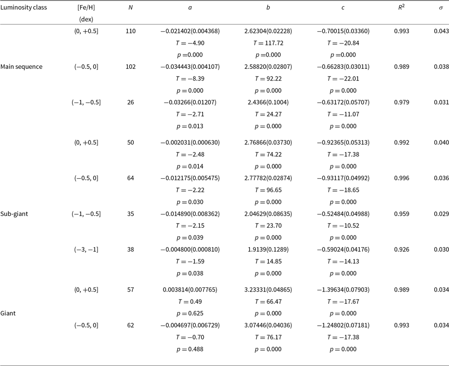
The numerical values of the coefficients a, b, and c estimated for 245 main sequence stars, 187 sub-giants, and 124 giants by using multiple regression method are given in Table 4. T and p values corresponding to the sensitivity of the coefficients are given in the third and fourth lines for each coefficient, while the squared correlation coefficients and the standard deviations are given in the last two columns of the table. One can see that the correlation coefficients are rather high, while the standard deviations are small. The residuals for the colour index  ${(U-V)_0}$
, the differences between the original colour indices and the estimated ones are rather small, and no systematic differences can be seen in their distribution (Figure 8). However, there is an exception for the giants, i.e. the uncertainty for the coefficient a is larger than itself, additionally the corresponding p value is greater than the usual one,
${(U-V)_0}$
, the differences between the original colour indices and the estimated ones are rather small, and no systematic differences can be seen in their distribution (Figure 8). However, there is an exception for the giants, i.e. the uncertainty for the coefficient a is larger than itself, additionally the corresponding p value is greater than the usual one,  ${p=0.05}$
.
${p=0.05}$
.
Coefficients derived from Equation (4) and the corresponding statistical results for sample stars of different luminosity classes and metallicities. N indicates the number of stars. The remaining symbols are explained in the text.
3.2. Transformation equations according to the luminosity classes and metallicities of stars
The sample stars are separated into different metallicity intervals, and transformation equations are derived for three luminosity classes of stars in each metallicity interval, as explained in the following. Main sequence and sub-giant stars occupy the metallicity intervals  ${0<{\rm [Fe/H]}\leq+0.5\text{ dex}}$
,
${0<{\rm [Fe/H]}\leq+0.5\text{ dex}}$
,  ${-0.5<{\rm [Fe/H]}\leq0\text{ dex}}$
,
${-0.5<{\rm [Fe/H]}\leq0\text{ dex}}$
,  ${-1<{\rm [Fe/H]}\leq-0.5\,\text{dex}}$
, additionally sub-giants occupy the interval
${-1<{\rm [Fe/H]}\leq-0.5\,\text{dex}}$
, additionally sub-giants occupy the interval  ${-3<{\rm [Fe/H]}\leq-1\text{ dex}}$
, while giants cover the metallicity intervals
${-3<{\rm [Fe/H]}\leq-1\text{ dex}}$
, while giants cover the metallicity intervals  ${0<{\rm [Fe/H]}\leq0.5\text{ dex}}$
and
${0<{\rm [Fe/H]}\leq0.5\text{ dex}}$
and  ${-0.5<{\rm [Fe/H]}\leq0\text{ dex}}$
. We used the Equation (4) and estimated the numerical values of the coefficients a, b, and c for each metallicity interval and luminosity class by the procedure explained in Section 3.1. Result are tabulated in Table 5. The squared correlation coefficients in this table are higher than those in Table 4. Also, the standard deviations in Table 4 reduced by 30%. Comparison of the observed
${-0.5<{\rm [Fe/H]}\leq0\text{ dex}}$
. We used the Equation (4) and estimated the numerical values of the coefficients a, b, and c for each metallicity interval and luminosity class by the procedure explained in Section 3.1. Result are tabulated in Table 5. The squared correlation coefficients in this table are higher than those in Table 4. Also, the standard deviations in Table 4 reduced by 30%. Comparison of the observed  ${{(U-V)_0}}$
colour indices and the estimated ones via Equation (4) is given in Figure 9. As it can be seen easily, there is no any systematic deviations in the distribution of residuals for
${{(U-V)_0}}$
colour indices and the estimated ones via Equation (4) is given in Figure 9. As it can be seen easily, there is no any systematic deviations in the distribution of residuals for  ${{(U-V)_0}}$
colour index. They are smaller than the those plotted in Figure 8, as well. However, we should note that the coefficient a estimated for the metallicity intervals of giants does not promise accurate
${{(U-V)_0}}$
colour index. They are smaller than the those plotted in Figure 8, as well. However, we should note that the coefficient a estimated for the metallicity intervals of giants does not promise accurate  ${{(U-V)_0}}$
colour index estimation.
${{(U-V)_0}}$
colour index estimation.
4. Summary and discussion
In this study, we used 556 stars with accurate spectroscopic, photometric, and astrometric data and derived transformation equations between GALEX and UBV colours. Thus, the U magnitudes of the stars would be estimated more accurately by means of FUV and NUV magnitudes which are observed outside of the Earth atmosphere. Transformation equations are derived as a function of (only) the luminosity class and as a function of both the luminosity class and metallicity. In both cases, the statistical results promise accurate  ${U-V}$
colours for the main sequence and sub-giant stars, estimated by using the FUV and NUV magnitudes. However, the same case does not hold for the giants.
${U-V}$
colours for the main sequence and sub-giant stars, estimated by using the FUV and NUV magnitudes. However, the same case does not hold for the giants.
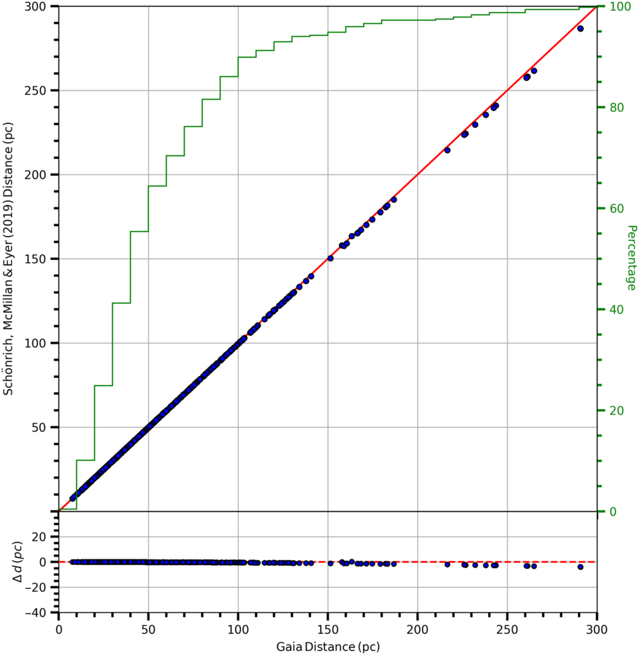
We used the inverted parallaxes as a distance estimate when calculating the interstellar absorption. However, Schönrich et al. (Reference Schönrich, McMillan and Eyer2019) have shown that the Gaia DR2 parallaxes can be biased. We compared the distances estimated via Gaia DR2 trigonometric parallaxes and the ones of Schönrich et al. (Reference Schönrich, McMillan and Eyer2019) which are obtained by a statistical method to see the impact of the distances of the stars on the analysis, as explained in the following. The mean of the differences between the distances estimated by two procedures and the corresponding standard deviation are  ${-0.10}$
pc and 0.66 pc, respectively. As seen in Figure 10, almost all distances fit with the one-to-one straight line. Hence, we do not expect any systematic uncertainty for our results.
${-0.10}$
pc and 0.66 pc, respectively. As seen in Figure 10, almost all distances fit with the one-to-one straight line. Hence, we do not expect any systematic uncertainty for our results.
Colour residuals for the sample stars in terms of  ${{(FUV-NUV)_0}}$
and
${{(FUV-NUV)_0}}$
and  ${{(B-V)_0}}$
colours for different luminosity classes and metallicities, as indicated in the panels. Dashed lines denote
${{(B-V)_0}}$
colours for different luminosity classes and metallicities, as indicated in the panels. Dashed lines denote  ${\pm 1\sigma}$
prediction levels.
${\pm 1\sigma}$
prediction levels.
Comparison of the distances for the sample stars estimated via Gaia DR2 trigonometric parallaxes and statistical method of Schönrich et al. (2019). The distances calculated by two different methods are quite compatible with one-to-one line.
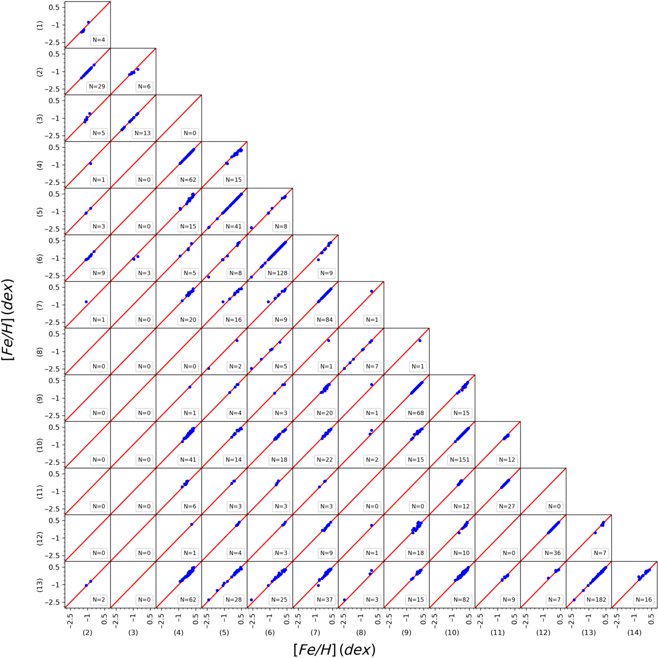
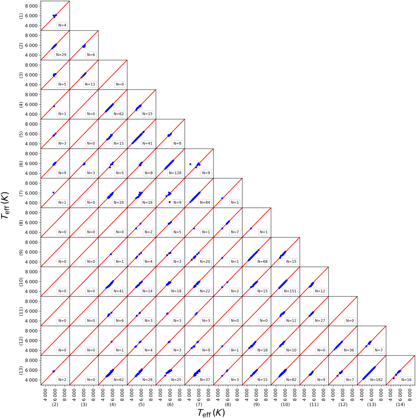
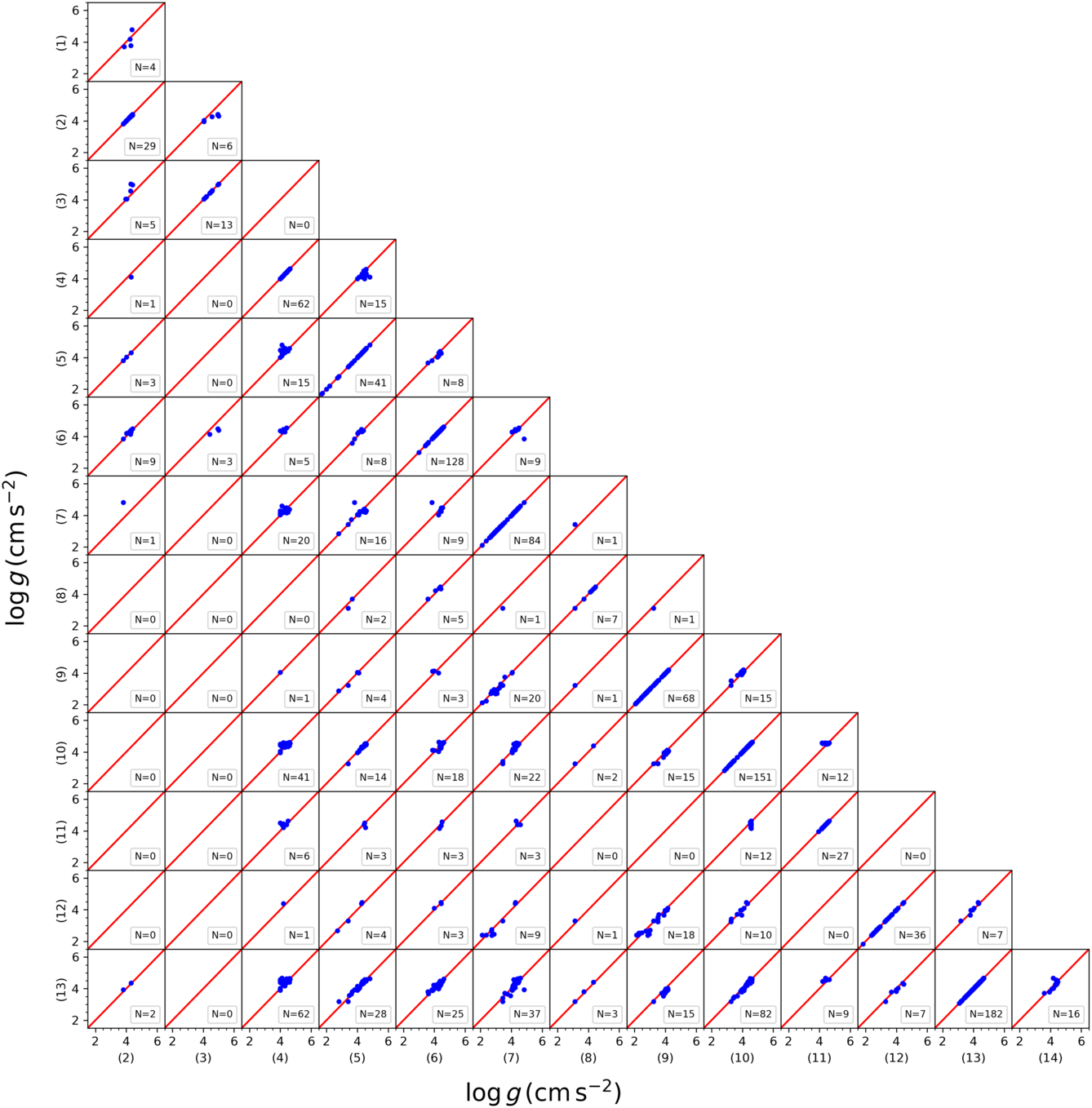
We compared the spectroscopic atmospheric model parameters taken from 14 different papers in the literature to investigate the confirmation of their homogeneity. Figures A1, A2, and A3 show that the three parameters,  ${T_{\rm eff}}$
,
${T_{\rm eff}}$
,  ${\log g}$
, and [Fe/H] lie on the one-to-one line in the corresponding figure. Hence, we can argue that the atmospheric model parameters taken from different studies are in an agreeable homogeneity.
${\log g}$
, and [Fe/H] lie on the one-to-one line in the corresponding figure. Hence, we can argue that the atmospheric model parameters taken from different studies are in an agreeable homogeneity.
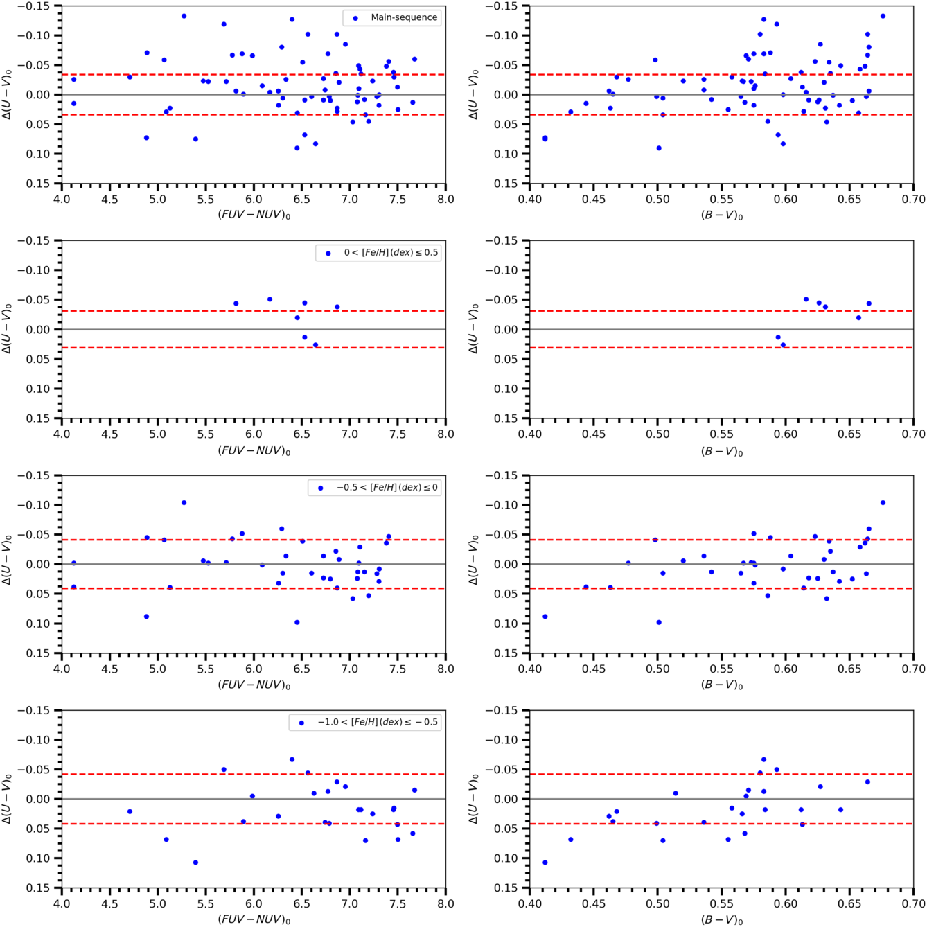
The transformation equations are applied to the F-G type main sequence stars Tunçel Güçtekin et al. (Reference Tunçel Güçtekin, Bilir, Karaali, Ak, Ak and Bostanc2016) which are provided with accurate photometric data. The sample of stars in the cited study reduced from 168 to 70 due to the absence of FUV and NUV magnitudes in GALEX DR7 (Bianchi et al. Reference Bianchi, Shiao and Thilker2017) database. We used the corresponding coefficients in Tables 4 and 5 and estimated the  ${{(U-V)_0}}$
colours of 70 stars in question. Residuals (Figure 11) and the statistical results (Table 6) show that combination of the luminosity class and metallicity provides more accurate
${{(U-V)_0}}$
colours of 70 stars in question. Residuals (Figure 11) and the statistical results (Table 6) show that combination of the luminosity class and metallicity provides more accurate  ${{(U-V)_0}}$
colours relative to the ones estimated by considering only the luminosity class. We should emphasize that the results corresponding only to the luminosity class are also consistent.
${{(U-V)_0}}$
colours relative to the ones estimated by considering only the luminosity class. We should emphasize that the results corresponding only to the luminosity class are also consistent.
Colour residuals for 70 main sequence stars taken from Tunçel Güçtekin et al. (Reference Tunçel Güçtekin, Bilir, Karaali, Ak, Ak and Bostanc2016) in terms of  ${{(FUV-NUV)_0}}$
(left column) and
${{(FUV-NUV)_0}}$
(left column) and  ${{(B-V)_0}}$
(right column). Residuals for stars with different metallicities are indicated in the panels. Dashed lines show
${{(B-V)_0}}$
(right column). Residuals for stars with different metallicities are indicated in the panels. Dashed lines show  ${{\pm 1\sigma}}$
prediction levels.
${{\pm 1\sigma}}$
prediction levels.
The transformation equations between the GALEX and UBV colours would be used for estimation of the U magnitude of stars for which this magnitude cannot be observed accurately. This is important for the intermediate spectral-type main sequence stars. Because the U magnitude thus obtained, i.e.  ${U_{\rm est}}$
, would be combined with the B magnitude of UBV photometric system and the
${U_{\rm est}}$
, would be combined with the B magnitude of UBV photometric system and the  ${U_{\rm est}-B}$
colour would be used in the (photometric) metallicity estimation which is important in studying the chemical structure and evolution of our Galaxy.
${U_{\rm est}-B}$
colour would be used in the (photometric) metallicity estimation which is important in studying the chemical structure and evolution of our Galaxy.
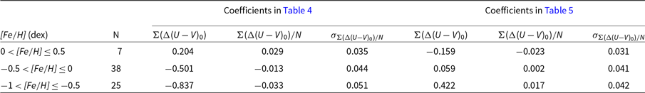
Statistical results based on the comparison of the observed and calculated  ${{(U-V)_0}}$
colours according to the coefficients in Tables 4 and 5 (sum of differences (
${{(U-V)_0}}$
colours according to the coefficients in Tables 4 and 5 (sum of differences ( ${\Sigma(\Delta (U-V)_0)}$
), means of differences (
${\Sigma(\Delta (U-V)_0)}$
), means of differences ( ${\Sigma(\Delta (U-V)_0)/N}$
), and standard deviations of differences
${\Sigma(\Delta (U-V)_0)/N}$
), and standard deviations of differences  ${\sigma_{\Sigma(\Delta (U-V)_0)/N}}$
) for 70 main sequence stars.
${\sigma_{\Sigma(\Delta (U-V)_0)/N}}$
) for 70 main sequence stars.
Acknowledgements
The authors thank the anonymous referee for her/his suggestions that helped improve the quality of the paper. This research has made use of NASA’s (National Aeronautics and Space Administration) Astrophysics Data System and the SIMBAD Astronomical Database, operated at CDS, Strasbourg, France, and NASA/IPAC Infrared Science Archive, which is operated by the Jet Propulsion Laboratory, California Institute of Technology, under contract with the National Aeronautics and Space Administration. This work has made use of data from the European Space Agency (ESA) mission Gaia (https://www.cosmos.esa.int/gaia), processed by the Gaia Data Processing and Analysis Consortium (DPAC, https://www.cosmos.esa.int/web/gaia/dpac/consortium ). Funding for the DPAC has been provided by national institutions, in particular the institutions participating in the Gaia Multilateral Agreement.
Corner plot showing a comparison of  ${T_{\rm eff}}$
for overlapping stars in 14 research groups. The numbers indicate the research groups: Boesgaard et al. (Reference Boesgaard2011), (2) Nissen & Schuster (Reference Nissen and Schuster2011), (3) Ishigaki et al. (Reference Ishigaki, Chiba and Aoki2012), (4) Mishenina et al. (Reference Mishenina, Pignatari, Korotin, Soubiran, Charbonnel, Thielemann, Gorbaneva and Basak2013), (5) Molenda-Zakowicz et al. (Reference Molenda-Zakowicz2013), (6) Bensby et al. (Reference Bensby, Feltzing and Oey2014), (7) da Silva et al. (Reference da Silva, Milone and Rocha-Pinto2015), (8) Sitnova et al. (Reference Sitnova2015), (9) Jofré et al. (Reference Jofré2015), (10) Brewer et al. (Reference Brewer, Fischer, Valenti and Piskunov2016), (11) Kim et al. (Reference Kim2016), (12) Maldonado & Villaver (Reference Maldonado and Villaver2016), (13) Luck (Reference Luck2017), (14) Delgado Mena et al. (Reference Delgado Mena, Tsantaki, Adibekyan, Sousa, Santos, Gonzalez Hernandez and Israelian2017).
${T_{\rm eff}}$
for overlapping stars in 14 research groups. The numbers indicate the research groups: Boesgaard et al. (Reference Boesgaard2011), (2) Nissen & Schuster (Reference Nissen and Schuster2011), (3) Ishigaki et al. (Reference Ishigaki, Chiba and Aoki2012), (4) Mishenina et al. (Reference Mishenina, Pignatari, Korotin, Soubiran, Charbonnel, Thielemann, Gorbaneva and Basak2013), (5) Molenda-Zakowicz et al. (Reference Molenda-Zakowicz2013), (6) Bensby et al. (Reference Bensby, Feltzing and Oey2014), (7) da Silva et al. (Reference da Silva, Milone and Rocha-Pinto2015), (8) Sitnova et al. (Reference Sitnova2015), (9) Jofré et al. (Reference Jofré2015), (10) Brewer et al. (Reference Brewer, Fischer, Valenti and Piskunov2016), (11) Kim et al. (Reference Kim2016), (12) Maldonado & Villaver (Reference Maldonado and Villaver2016), (13) Luck (Reference Luck2017), (14) Delgado Mena et al. (Reference Delgado Mena, Tsantaki, Adibekyan, Sousa, Santos, Gonzalez Hernandez and Israelian2017).
Corner plot showing a comparison of  ${\log g}$
for overlapping stars in 14 research groups. The numbers indicate the research groups as in Figure A1.
${\log g}$
for overlapping stars in 14 research groups. The numbers indicate the research groups as in Figure A1.
Corner plot showing a comparison of [Fe/H] for overlapping stars in 14 research groups. The numbers indicate the research groups as in Figure A1.