


1. Introduction
Many populations worldwide have experienced significant mortality improvements throughout the last decades, and human mortality has shifted to later ages (see Vaupel et al. Reference Vaupel, Villavicencio and Bergeron-Boucher2021). The advancement of the longevity frontier implies compelling financial challenges for individuals aiming to manage their post-retirement income, as well as for annuity providers. Individuals living longer face the risk of outliving their wealth, and at least theoretically, they should look at the standard life annuity as an optimal vehicle for insuring against the individual longevity risk (Yaari Reference Yaari1965). But in reality, the voluntary annuity market remains thin because of rational and behavioural individual reasons driving the life annuities demand (see, e.g., Brown Reference Brown2001; Reference Brown2009). The downward trend in mortality rates, jointly with the uncertainty of financial markets and the evolving demographic structure of many populations, has led social security schemes and pension funds to revise pension benefits downwards. The shift from Defined Benefit to Defined Contribution plans has also taken hold. Consequently, individuals remain exposed to both individual investment and longevity risks; transferring such risks to a private annuity provider should be perceived as a beneficial strategy for building a suitable and stable retirement income. However, on their side, life insurers suffer the cost of financial and longevity guarantees traditionally embedded in life annuities, and they have become averse to offering non-adjustable longevity guarantees. The aggregate longevity risk cannot be diversified through risk pooling strategies and could require considerable equity capital backing due to risk-based solvency regulations. Then, academics and practitioners have examined alternative longevity risk management solutions. For instance, Blake et al. (Reference Blake, Cairns and Dowd2006) discuss how annuity providers can use mortality/longevity-linked securities to handle the risk of uncertain aggregate mortality. Even with great potential, the demand for the capital market securities proposed over the last decade has been very low, and annuity providers mainly relied on insurance-based solutions, such as buy-outs, buy-ins and insurance-based longevity swaps (Blake et al. Reference Blake, Cairns, Dowd and Kessler2019). Non-financial longevity reinsurance may also be considered, but it is usually costly and ultimately has to be funded by higher insurance premiums. As a workable alternative, longevity-linked arrangements have been proposed in the literature (see, e.g, Olivieri and Pitacco Reference Olivieri and Pitacco2020). Beyond the specific design of these products, the underlying idea is that the insurer shares the risk with the policyholder by linking the life annuity benefits, directly or indirectly, to the mortality experience of a reference population. If unexpected mortality improvements occur, the insurer can mitigate its longevity risk exposure, but in the meantime, the benefits amount would decrease, likely hurting the demand for such insurance products.
Each longevity risk management solution has drawbacks, and insurers are motivated to modify their products by partially shifting risks to the policyholder. In the recent actuarial literature, notable attention has been given to pooling designs as innovative risk-sharing mechanisms to support the post-retirement income of individuals. Their common feature consists of grouping individuals to create a fund, from which each participant will receive periodical benefits adjusted according to the investment returns and mortality experienced by the pool, with no guarantee embedded. As a result, pool participants share among themselves the financial and longevity risk, and the insurer could play the role of administrator, not a guarantor (Dhaene and Milevsky Reference Dhaene and Milevsky2024). Different pooling structures have been proposed in the literature, such as the pooled annuity funds (see, e.g., Donnelly et al., Reference Donnelly, Montserrat and Nielsen2014; Donnelly, Reference Donnelly2015), and tontine annuities (see, e.g., Milevsky and Salisbury, Reference Milevsky and Salisbury2015; Chen et al., Reference Chen, Hieber and Klein2019; Weinert and Grüundl, 2021; Chen et al., Reference Chen, Chen and Xu2022; Hieber and Lucas, Reference Hieber and Lucas2022) among others.
In the present work, we refer to one of the earlier pooling structures, namely the group self-annuitisation (GSA). Introduced by Piggott et al. (Reference Piggott, Valdez and Detzel2005), a GSA scheme is a mutual insurance plan wherein individuals are brought together to pool both their investment and longevity risks. Individuals joining the GSA scheme pay an initial contribution determined according to an annuity payout rate. Therefore, the benefits that GSA members receive periodically account for both the expected mortality dynamics and the expected return on investments. Considering that the pool is required to fully cover its liabilities with its own assets at all times, future benefits have to be adjusted if the actual mortality and/or the realised investments return diverge from their respective expectations. Qiao and Sherris (Reference Qiao and Sherris2013) further study the GSA plan by assessing its effectiveness when systematic longevity risk is also considered. Shedding light on the investment activity of GSA plans, Olivieri et al. (Reference Olivieri, Thirurajah and Ziveyi2022) propose a dynamic target volatility strategy to enhance the survival benefits of the pool participants. Kabuche et al. (Reference Kabuche, Sherris, Villegas and Ziveyi2024) expand the GSA structure, allowing group participants to share both longevity and health risks. To this end, a multi-state GSA plan is proposed to pool heterogeneous individuals and provide annuity benefits updated according to both realised health transitions and mortality experienced. Aragona et al. (Reference Aragona, Regis and Vigna2025) introduce a redistributive GSA fund aiming to optimally share benefits among heterogeneous participants belonging to different socio-economic classes.
There is a growing attention, both in the market and literature, towards annuity and pooling designs providing differentiated benefits by health status, as a lever to foster annuitisation. The background assumption is that individuals who feel to have a shorter life expectancy, due to illnesses or lifestyle habits, may be reluctant to opt into a standard plan, while they might find it convenient to join arrangements that pay higher benefits should a shorter life expectancy be ascertained. Special rate (or underwritten or substandard) annuities are designed to respond to such a preference (see, for example, Pitacco and Tabakova Reference Pitacco and Tabakova2022; Ramsay et al. Reference Ramsay, Oguledo and Krutto2025; de Andrés-Sánchez and González-Vila Puchades Reference de Andrés-Sánchez and González-Vila Puchades2025); in the context of self-insured plans, the pooling arrangement proposed by Kabuche et al. (Reference Kabuche, Sherris, Villegas and Ziveyi2024) is also suitable in this respect.
Against this background, we propose a multi-state framework that explicitly incorporates the mortality heterogeneity characterising GSA members, with the objective of defining a design admitting a benefit differentiation. Our focus, in particular, is on whether the GSA scheme should differentiate benefits so that frailer individuals (with shorter life expectancy and presumably greater current financial needs, due to higher healthcare or care-related expenses) receive higher payments than healthier individuals (who are expected to cash benefits for a longer time).
Individual mortality is influenced by various elements, such as current health status, lifestyles, socio-economic conditions and climate characteristics. Each of these elements could significantly reshape the lifespan of individuals, and in particular, the timing of their ageing. In this paper, we refer to ageing as a continuous-time deterioration process of the human physiological functions necessary for survival. Individuals could bear a series of ageing phases before dying, and the speed at which ageing progresses varies from person to person, generating heterogeneity in the mortality of a population. While in a traditional GSA scheme benefits are adjusted based on aggregate realised mortality, we aim to design a GSA in which benefit adjustments account for both realised ageing transitions and mortality. Accordingly, a mortality model that explicitly accounts for the ageing process must be considered.
Individual’s ageing does not necessarily move in lockstep with calendar time. The so-called biological age is an example of this, that is, the age indicating how old the human mechanism is at both the cellular and molecular levels (see, e.g., Jackson et al. Reference Jackson, Weale and Weale2003). Biological age is usually determined with a microscopic approach, that is, by collecting data concerning physiological and molecular variables for a large sample of people, and, through regression techniques, an increment or a reduction of the corresponding chronological age is inferred. We refer the interested reader to Li et al. (Reference Li, Zhang, Duan, Niu, Chen, Liu, Dong, Zheng, Chen, Feng, Wang, Zhao, Sun, Cai, Jiang and Chen2023) for a discussion on the methods proposed in the literature for calculating biological age; we also refer the reader to Milevsky (Reference Milevsky2020) for an actuarial view on using biological age in mortality analysis. The biological age measurement requires high data granularity, and it is subject to both data collection and processing times. In contrast, annuity providers, as well as the administrators of a pooling fund, usually have access to mortality data only at an aggregate level, without having the possibility to observe biological factors. When there are no detectable biological factors other than age, the ageing process can still be represented, with the so-called Markov ageing model (see Lin and Liu Reference Lin and Liu2007; Liu and Lin Reference Liu and Lin2012; Su and Sherris Reference Su and Sherris2012; Cheng et al. Reference Cheng, Jones, Liu and Ren2020). It is a finite-state continuous-time Markov process suitable for modelling the human ageing evolution. Each state of the Markov process identifies an ageing phase, and the overall ageing process is described through consecutive transitions from one ageing state to a higher one. An absorbing (death) state is also included, and the transition from any ageing state to the absorbing state represents the ageing process termination due to death. The Markov ageing model allows for linking directly the age-specific mortality pattern to the ageing process, and the intrinsic heterogeneity of a cohort can be expressed explicitly. In addition, the stochastic process has desirable analytical properties suitable for mortality analysis.
We define a pooling design, which we refer to as a Markov ageing GSA, in which individuals joining the pool are classified according to their initial ageing state, and their ageing trajectory is reassessed annually. Benefits are differentiated by state; upon transitioning to a higher ageing state, the individual’s benefit is topped up to the level associated with the new state. Each individual contributes an initial capital assessed accounting for the initial state, the expected transition to higher ageing states and to the death state, as well as for the expected investment return. For the sake of simplicity, we assume a deterministic financial setting and a constant return on investments. This enables us to isolate and examine the effects on the benefit profile of the uncertain mortality dynamics in a context of a heterogeneous population. Similarly to a plain GSA, to preserve the actuarial equivalence between benefits and available resources, benefits are adjusted annually if experience deviates from expectation. In our setting, we account for both the realised ageing process pattern and actual mortality. Benefit adjustments are state-specific; any deficit or surplus arising from deviations between expected and realised experience is allocated across states in a way that reflects both the relative value of obligations in each state and the potential severity of deviations within each state. In a first phase of the analysis, benefit differentiation and adjustments are defined so to ensure actuarial equivalence for each state. To this end, making cross-subsidy mechanisms between states explicit is crucial. However, as noted above, the ageing process is not directly observable at the individual level but must be inferred from proxy factors, such as the onset of disabling illnesses or the worsening of lifestyle behaviours. This is a critical issue, in respect of both suitability of the proxy risk factors and potential self-interested behaviours by individuals. Participants, in particular, may have specific targets regarding the degree of benefit differentiation, which are not necessarily ensured by an actuarially equivalent adjustment mechanism. In a second phase of the analysis, we explore the adoption of benefits that are differentiated by the states identified by proxy risk factors (rather than the ageing states) and that keep a predetermined scaling factor between them, chosen according to the desired level of differentiation. Both choices introduce solidarity mechanisms, which we can highlight by comparing the resulting benefits with the ones grounded on actuarial equivalence by ageing state. Our work differs from previous contributions on this topic, such as Kabuche et al. (Reference Kabuche, Sherris, Villegas and Ziveyi2024), in two regards. First, the use of a Markov ageing model allows us to incorporate latent heterogeneity that cannot be directly measured. Second, we address explicitly possible solidarity mechanisms, identifying their magnitude. Understanding the degree of solidarity built into the system is fundamental to ensure transparency and to make any redistribution a deliberate and justifiable design choice. We develop our proposal referring to a GSA closed to the entry of new cohorts. This allows us to understand the extent to which accounting for mortality heterogeneity leads to efficient mortality risk pooling within a single cohort. We test our theoretical framework through a numerical application using a 5-state Markov ageing model and referring to Australian mortality data for both genders. Our findings support that individual longevity risk can be effectively pooled under population heterogeneity, allowing for differentiated benefits reflecting differences in participants’ life expectancies. Our results also indicate that actuarial equivalence requires a sufficiently large population size, whereas implementing solidarity mechanisms may be justified. Indeed, the estimated benefits profile appears generally stable, apart from state-specific fluctuations when the cohort shrinks to a low size. The severity of ageing significantly drives the dynamics of benefits. The last ageing state’s benefit profile is increasing on average; conversely, the intermediate ageing states’ benefit profile, as well as the first, tends to decrease as the maximum duration of the scheme is approached. Such evidence bolsters the introduction of explicit solidarity mechanisms to avoid disincentivising the participation of individuals with better physiological statuses. Then, we numerically investigate the effect of solidarity rules on rearranging benefit levels and preserving the actuarial equivalence between benefits and available resources. Depending on the number of benefit levels the scheme would provide, the benefit profile may increase more or less marked over time and in a consistent way across states, while remaining reasonably differentiated among frailer and healthier individuals.
The paper is organised as follows. In Section 2, we describe in detail the Markov ageing model. In Section 3, we present the actuarial design of the multi-state GSA, in particular addressing cross-subsidies across states and the introduction of solidarity. In Section 4, a numerical application of the proposed theoretical framework is provided, as well as a discussion of the main findings. Finally, Section 5 concludes with some final remarks.
2. The Markov ageing model
Let $\left(A_t, \, t\geq0\right)$
be a finite-state continuous-time homogeneous Markov process describing the ageing evolution of a population, and let
$\left(A_t, \, t\geq0\right)$
be a finite-state continuous-time homogeneous Markov process describing the ageing evolution of a population, and let $E=\left\{1,2,\ldots,m\right\}$
, with
$E=\left\{1,2,\ldots,m\right\}$
, with $m \in \mathbb{N}_{\gt1}$
, be the set of transient states. Each of them identifies an ageing state or phase. The process takes values on the finite state-space
$m \in \mathbb{N}_{\gt1}$
, be the set of transient states. Each of them identifies an ageing state or phase. The process takes values on the finite state-space $\mathcal{S}=E\cup\{m+1\}$
, where
$\mathcal{S}=E\cup\{m+1\}$
, where $m+1$
represents the death (absorbing) state. The infinitesimal generator of
$m+1$
represents the death (absorbing) state. The infinitesimal generator of $\left(A_t, \, t\geq0\right)$
is
$\left(A_t, \, t\geq0\right)$
is
 \begin{equation} {} {} {} {}\boldsymbol{\Sigma} = \begin{pmatrix} {} {} {}\boldsymbol{\Lambda} \;\;\;\;\;& \boldsymbol{q} \\ {} {} {}\boldsymbol{0}\;\;\;\;\; & 0 {} {}\end{pmatrix} \in \mathbb{R}^{(m+1) \times (m+1)}, {}\end{equation}
where $\boldsymbol{\Lambda}$
is the
$\boldsymbol{\Lambda}$
is the $m\times m$
intensity matrix and
$m\times m$
intensity matrix and $\boldsymbol{q}=-\boldsymbol{\Lambda}\boldsymbol{e}$
is a m-dimensional column vector of transition intensities to the death state, with
$\boldsymbol{q}=-\boldsymbol{\Lambda}\boldsymbol{e}$
is a m-dimensional column vector of transition intensities to the death state, with $\boldsymbol{e}$
a column vector of ones.
$\boldsymbol{e}$
a column vector of ones.
Let $\boldsymbol{\pi}=\left(\pi_1,\pi_2,\ldots,\pi_m\right)$
be a probability vector stating the initial distribution of the process, with
$\boldsymbol{\pi}=\left(\pi_1,\pi_2,\ldots,\pi_m\right)$
be a probability vector stating the initial distribution of the process, with $\pi_i\;:\!=\;\mathbb{P}\left(A_0=i\right)\geq0, \, i \in E$
, and
$\pi_i\;:\!=\;\mathbb{P}\left(A_0=i\right)\geq0, \, i \in E$
, and $\mathbb{P}\left(A_0=m+1\right)=0$
. Since the Markov process has only one absorbing state, the time until death is defined as
$\mathbb{P}\left(A_0=m+1\right)=0$
. Since the Markov process has only one absorbing state, the time until death is defined as
 \begin{equation} {} {} {} {}\tau \;:\!=\; \inf\left\{t\gt0 \, : \, A_t=m+1\right\}, {}\end{equation}
and follows a phase-type (PH) distribution with representation $\left(\boldsymbol{\pi},\boldsymbol{\Lambda}\right)$
, that is,
$\left(\boldsymbol{\pi},\boldsymbol{\Lambda}\right)$
, that is, $\tau \sim \text{PH}\left(\boldsymbol{\pi},\boldsymbol{\Lambda}\right)$
. In particular, we deal with a generalised Coxian PH distribution so that the intensity matrix is written in the following form:
$\tau \sim \text{PH}\left(\boldsymbol{\pi},\boldsymbol{\Lambda}\right)$
. In particular, we deal with a generalised Coxian PH distribution so that the intensity matrix is written in the following form:
 \begin{equation} {} {} {} {}\renewcommand\arraystretch{1.5} {} {}\boldsymbol{\Lambda}=\begin{pmatrix} {} {} {}-\left(\lambda_1+q_1\right) & \quad \lambda_1 & \quad 0 & \quad \cdots & \quad 0 \\ {} {} {}0 & \quad -\left(\lambda_2+q_2\right) & \quad \lambda_2 & \quad \cdots & \quad 0 \\ {} {} {}0 & \quad 0 & \quad -\left(\lambda_3+q_3\right) & \quad \cdots & \quad 0 \\ {} {} {}\vdots & \quad \vdots & \quad \vdots & \quad \ddots & \quad \vdots \\ {} {} {}0 & \quad 0 & \quad 0 & \quad \cdots & \quad -q_m {} {}\end{pmatrix}, {}\end{equation}
being $\lambda_i\geq0$
the transition intensity from the ageing state i to the next ageing state, while
$\lambda_i\geq0$
the transition intensity from the ageing state i to the next ageing state, while $q_i\gt0$
is the transition rate into the absorbing state. The generalised Coxian PH distribution is particularly attractive due to its mathematical tractability and explainability. As shown by the phase diagram in Figure 1, the ageing process is described through a sequence of ageing phases, following a lexicographical order, and the death event may occur with a certain probability in the meantime. The sojourn time in the ageing phase i is exponentially distributed with rate
$q_i\gt0$
is the transition rate into the absorbing state. The generalised Coxian PH distribution is particularly attractive due to its mathematical tractability and explainability. As shown by the phase diagram in Figure 1, the ageing process is described through a sequence of ageing phases, following a lexicographical order, and the death event may occur with a certain probability in the meantime. The sojourn time in the ageing phase i is exponentially distributed with rate $\lambda_i+q_i$
, and, for
$\lambda_i+q_i$
, and, for $i=1,\ldots,m-1$
, the process moves to the ageing phase
$i=1,\ldots,m-1$
, the process moves to the ageing phase $i+1$
with probability
$i+1$
with probability $\frac{\lambda_i}{\lambda_i+q_i}$
; otherwise, the ageing process terminates due to the death occurrence with probability
$\frac{\lambda_i}{\lambda_i+q_i}$
; otherwise, the ageing process terminates due to the death occurrence with probability $\frac{q_i}{\lambda_i+q_i}$
. As ageing progresses, the physiological status of the population deteriorates, implying a greater probability of approaching the absorbing state. In particular, when
$\frac{q_i}{\lambda_i+q_i}$
. As ageing progresses, the physiological status of the population deteriorates, implying a greater probability of approaching the absorbing state. In particular, when $i=m$
, the probability of jumping to the death state is 1.
$i=m$
, the probability of jumping to the death state is 1.
Generalised Coxian distribution’s phase diagram.

A key issue in adopting a PH distribution concerns the dimension of $\boldsymbol{\Lambda}$
. The PH representation
$\boldsymbol{\Lambda}$
. The PH representation $\left(\boldsymbol{\pi},\boldsymbol{\Lambda}\right)$
is highly parameterised and non-uniqueness problems in parameter specifications could emerge (see, e.g., Asmussen et al. Reference Asmussen, Nerman and Olsson1996). As m increases, numerical issues may also arise in estimating parameters
$\left(\boldsymbol{\pi},\boldsymbol{\Lambda}\right)$
is highly parameterised and non-uniqueness problems in parameter specifications could emerge (see, e.g., Asmussen et al. Reference Asmussen, Nerman and Olsson1996). As m increases, numerical issues may also arise in estimating parameters $\lambda_i$
and
$\lambda_i$
and $q_i$
. Focusing on modelling the human mortality schedule, the PH distribution could require a high dimension of the intensity matrix. For instance, Lin and Liu (Reference Lin and Liu2007) adopt the Coxian distribution to fit the mortality schedule from age 0 to age 100, suggesting that 200–250 ageing phases are needed. Cheng et al. (Reference Cheng, Jones, Liu and Ren2020) impose specific structures on
$q_i$
. Focusing on modelling the human mortality schedule, the PH distribution could require a high dimension of the intensity matrix. For instance, Lin and Liu (Reference Lin and Liu2007) adopt the Coxian distribution to fit the mortality schedule from age 0 to age 100, suggesting that 200–250 ageing phases are needed. Cheng et al. (Reference Cheng, Jones, Liu and Ren2020) impose specific structures on $\lambda_i$
and
$\lambda_i$
and $q_i$
, finding that 100 phases are pretty reasonable in fitting mortality data. Conversely, Liu and Lin (Reference Liu and Lin2012) argue that if only part of the mortality schedule is relevant, for example, from age 65 onwards, a lower-dimensional PH distribution is enough to achieve an accurate fit. Such an approach could be suitable for our purposes, since we deal with ages falling within the post-retirement life of individuals. Further details concerning the Markov ageing model fitting will be provided in Section 4.
$q_i$
, finding that 100 phases are pretty reasonable in fitting mortality data. Conversely, Liu and Lin (Reference Liu and Lin2012) argue that if only part of the mortality schedule is relevant, for example, from age 65 onwards, a lower-dimensional PH distribution is enough to achieve an accurate fit. Such an approach could be suitable for our purposes, since we deal with ages falling within the post-retirement life of individuals. Further details concerning the Markov ageing model fitting will be provided in Section 4.
Denoting with $p^{i,j}_t = \mathbb{P}\left(A_t=j | A_0=i\right)$
the time-homogeneous transition probability from the ageing state i to the ageing state j, the transition probability matrix, namely
$p^{i,j}_t = \mathbb{P}\left(A_t=j | A_0=i\right)$
the time-homogeneous transition probability from the ageing state i to the ageing state j, the transition probability matrix, namely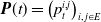 $\boldsymbol{P}(t)=\left(p^{i,j}_t\right)_{i,\, j \in E}$
, satisfies the following Kolmogorov forward equation:
$\boldsymbol{P}(t)=\left(p^{i,j}_t\right)_{i,\, j \in E}$
, satisfies the following Kolmogorov forward equation:
 \begin{equation} {} {} {} {}\displaystyle\frac{d}{dt} \boldsymbol{P}(t) =\boldsymbol{P}(t)\boldsymbol{\Lambda}, {}\end{equation}
with the initial condition $\boldsymbol{P}(0)=\boldsymbol{I}$
, where
$\boldsymbol{P}(0)=\boldsymbol{I}$
, where $\boldsymbol{I}$
is the identity matrix. Equation (2.4) admits a unique solution given by
$\boldsymbol{I}$
is the identity matrix. Equation (2.4) admits a unique solution given by
 \begin{equation} {} {}\boldsymbol{P}(t)=\exp(\boldsymbol{\Lambda} t), {}\end{equation}
where the exponential matrix is defined by series expansion, that is, $\exp\left(\boldsymbol{\Lambda}t\right)=\sum_{h=0}^{\infty}\frac{\left(t\boldsymbol{\Lambda}\right)^h}{h!}$
.
$\exp\left(\boldsymbol{\Lambda}t\right)=\sum_{h=0}^{\infty}\frac{\left(t\boldsymbol{\Lambda}\right)^h}{h!}$
.
Under the PH distributions, many quantities of interest concerning the future lifetime are available in closed form. For instance, the survival function for a newborn can be written as:
 \begin{equation} {} {} {} {}S_0(t) = \boldsymbol{\pi}^\top\exp\left(\boldsymbol{\Lambda}t\right)\boldsymbol{e}, \quad t\gt0. {}\end{equation}
Moreover, the conditional survival function given the survival at age $x\gt0$
is
$x\gt0$
is
 \begin{equation} {} {} {} {}S_x(t) = \frac{S_0(x+t)}{S_0(x)} = \frac{\boldsymbol{\pi}^\top\exp\left(\boldsymbol{\Lambda}(x+t)\right)\boldsymbol{e}}{\boldsymbol{\pi}^\top\exp\left(\boldsymbol{\Lambda}x\right)\boldsymbol{e}} = \boldsymbol{\pi}^\top_x\exp\left(\boldsymbol{\Lambda}t\right)\boldsymbol{e}, \quad t\gt0, {}\end{equation}
where $\boldsymbol{\pi}_x^\top = \frac{\boldsymbol{\pi}^\top\exp\left(\boldsymbol{\Lambda}x\right)}{\boldsymbol{\pi}^\top\exp\left(\boldsymbol{\Lambda}x\right)\boldsymbol{e}}$
represents the distribution of the ageing phases, given the survival at age x.
$\boldsymbol{\pi}_x^\top = \frac{\boldsymbol{\pi}^\top\exp\left(\boldsymbol{\Lambda}x\right)}{\boldsymbol{\pi}^\top\exp\left(\boldsymbol{\Lambda}x\right)\boldsymbol{e}}$
represents the distribution of the ageing phases, given the survival at age x.
Remark 2.1. In the Markov ageing model, once the process leaves an ageing state, it is impossible to return to it. In other words, the Markov ageing model keeps track of the ageing progression in the forward sense, and possible rejuvenations are not considered. Rejuvenation may be biologically possible only following various lifestyle interventions concerning nutrition, physical exercise and the social environment (see, e.g., Félix et al. Reference Félix, Martnez de Toda and Daz-Del Cerro2024). Detailed information at the individual level is crucial to assessing the significance of possible rejuvenation transitions. As explained in Section 1, such data granularity is often unavailable to annuity providers, and rejuvenation transitions cannot be estimated.
To assist the reader, notation adopted in the current section is resumed in Table 1.
Notation, and related meaning, adopted for describing the Markov ageing model.

3. The Markov ageing GSA arrangement
3.1 Pool structure
We consider a GSA scheme that provides post-retirement benefits to its members. Individuals pay an initial capital when joining the scheme; upon death, any residual amount is retained by the pool (i.e., no death benefit is included). In return for their initial contribution, members receive an annual lifetime income, whose amount is differentiated depending on the specific mortality profile of the individual. In fact, the GSA is structured with multiple levels of benefits, with higher benefit amounts provided to those with a shorter life expectancy. The individual’s mortality profile is first assessed at entry and then reviewed annually. Upon a change of the mortality profile, for example, following the onset of a disease, the individual will be assigned the level of benefit consistent with his(her) new status. However, similarly to a traditional GSA, annual amounts for the various benefit levels are not guaranteed but are subject to annual adjustment based on the investment and longevity experience of the pool. In the following, we focus on longevity only, and we propose an approach to define such adjustments, which is motivated by actuarial arguments.
Mortality is modelled adopting the Markov ageing setting described in Section 2. We first assume that it is possible to classify individuals according to the ageing states and to differentiate benefits based on such states. However, as already pointed out in Section 1, biological age (which is at the root of ageing states) is not directly measurable. In the second step of the discussion (in particular, in Section 3.5), we assume that individuals are classified according to proxy risk factors. It is unlikely that risk classes identified this way correspond exactly to the ageing states of the Markov model. The implications are discussed in Section 3.5; for the moment, we assume that both at entry and at any time, a risk classification based on the ageing states of the Markov model can be performed. In particular, we assume that it is possible to describe the dynamics of each individual’s mortality profile in terms of the transition to higher ageing states.
We consider a single cohort consisting of $L_x$
individuals who join the scheme at time
$L_x$
individuals who join the scheme at time $t=0$
, at chronological age x, with
$t=0$
, at chronological age x, with $L_x^i$
individuals placed in state i,
$L_x^i$
individuals placed in state i, $i\in E$
(clearly,
$i\in E$
(clearly, $\sum_{i=1}^m L_x^i=L_x$
). The maximum attainable age is
$\sum_{i=1}^m L_x^i=L_x$
). The maximum attainable age is $\omega$
for each individual; however, we assume that, to avoid the impact of major random fluctuations at later ages (when the cohort will shrink to low size), the scheme is committed to pay benefits up to time
$\omega$
for each individual; however, we assume that, to avoid the impact of major random fluctuations at later ages (when the cohort will shrink to low size), the scheme is committed to pay benefits up to time $t_{\max}$
(i.e., up to chronological age
$t_{\max}$
(i.e., up to chronological age $x_{\max}=x+t_{\max}\lt\omega$
). At time
$x_{\max}=x+t_{\max}\lt\omega$
). At time $t_{\max}$
, the available funds will be transferred to an insurer willing to take charge of the surviving participants and their funds and guarantee them a lifetime annuity. The price and optimal time of such a transfer (which undoubtedly constitute interesting research questions) are not addressed in this paper, as our aim for now is to define acceptable benefit adjustment rules when multiple levels of benefits are involved; addressing also the transfer at time
$t_{\max}$
, the available funds will be transferred to an insurer willing to take charge of the surviving participants and their funds and guarantee them a lifetime annuity. The price and optimal time of such a transfer (which undoubtedly constitute interesting research questions) are not addressed in this paper, as our aim for now is to define acceptable benefit adjustment rules when multiple levels of benefits are involved; addressing also the transfer at time $t_{\max}$
would excessively broaden the scope of the present study. Thus, in this paper, we simply assume that the scheme will pay an income to survivors at times
$t_{\max}$
would excessively broaden the scope of the present study. Thus, in this paper, we simply assume that the scheme will pay an income to survivors at times $t=0,1,\ldots,t_{\max}$
, for a chosen (reasonable)
$t=0,1,\ldots,t_{\max}$
, for a chosen (reasonable) $t_{\max}$
, and the scheme’s payout rate will not account for annuity costs concerning times
$t_{\max}$
, and the scheme’s payout rate will not account for annuity costs concerning times $t\gt t_{\max}$
.
$t\gt t_{\max}$
.
Let $B_0^{i}$
be the benefit set at time
$B_0^{i}$
be the benefit set at time $t=0$
for state
$t=0$
for state $i \in E$
. An individual entering the scheme in state i will initially get the benefit
$i \in E$
. An individual entering the scheme in state i will initially get the benefit $B_0^i$
; however, upon transition to a state
$B_0^i$
; however, upon transition to a state $j\gt i$
,
$j\gt i$
, $j\in E$
, (s)he is entitled to cash the benefit
$j\in E$
, (s)he is entitled to cash the benefit $B_0^{j}$
. Based on the usual actuarial arguments, the initial capital to be paid by an individual in state i at time
$B_0^{j}$
. Based on the usual actuarial arguments, the initial capital to be paid by an individual in state i at time $t=0$
is then assessed as follows:
$t=0$
is then assessed as follows:
 \begin{equation} {} {}V_0^{i} = \sum_{j\geq i}^{m} B_0^{j}\, \ddot{a}^{i,j}_{x}, {}\end{equation}
where $\ddot{a}^{i,j}_{x} = \sum_{h=0}^{t_{\max}}(1+r)^{-h} {_hp_x^{i,j}}$
is the actuarial value of the annuity paid when in state j, computed using the transition probabilities
$\ddot{a}^{i,j}_{x} = \sum_{h=0}^{t_{\max}}(1+r)^{-h} {_hp_x^{i,j}}$
is the actuarial value of the annuity paid when in state j, computed using the transition probabilities $_hp_x^{i,j}=\exp(\boldsymbol{\Lambda}h)_{i,j}$
predicted by the mortality model and a given (deterministic) discount rate r. We point out that no loading is embedded in the choice of parameters of (3.1), as it is natural for a GSA scheme. We note also that the differentiation by state concerns not only the benefits but, consistently, the initial capital too.
$_hp_x^{i,j}=\exp(\boldsymbol{\Lambda}h)_{i,j}$
predicted by the mortality model and a given (deterministic) discount rate r. We point out that no loading is embedded in the choice of parameters of (3.1), as it is natural for a GSA scheme. We note also that the differentiation by state concerns not only the benefits but, consistently, the initial capital too.
3.2 Pool funds
A GSA is grounded on the principle of funded liabilities. In other words, it is required that a balance be maintained at all times between available resources and the value of obligations. This is achieved by updating the benefit amount, upwards or downwards, depending on the experience with longevity and investments. We assume that the adjustment is applied annually, right before the benefit is paid at time t, $t\geq 1$
. Let
$t\geq 1$
. Let $B_0^i$
be the benefit set at time
$B_0^i$
be the benefit set at time $t=0$
for state
$t=0$
for state $i\in E$
; reasonably,
$i\in E$
; reasonably, $B_0^1\lt B_0^2\lt\ldots\lt B_0^m$
, since higher-indexed states correspond to lower life expectancy. Taking
$B_0^1\lt B_0^2\lt\ldots\lt B_0^m$
, since higher-indexed states correspond to lower life expectancy. Taking $B_0^1$
as the baseline benefit amount, it may be convenient to express the initial benefit amount for each state
$B_0^1$
as the baseline benefit amount, it may be convenient to express the initial benefit amount for each state $i, i\gt1$
, as a proportion of
$i, i\gt1$
, as a proportion of $B_0^1$
, as follows:
$B_0^1$
, as follows: $B_0^i=c^i B_0^1$
, where the
$B_0^i=c^i B_0^1$
, where the $c^i$
’s (
$c^i$
’s ( $1\lt c^2\lt c^3\lt\ldots\lt c^m$
) are chosen according to some target. We let
$1\lt c^2\lt c^3\lt\ldots\lt c^m$
) are chosen according to some target. We let $B_t^{i}$
denote the updated benefit amount at time t for state i, according to an adjustment rule which is described in Section 3.4. In the following, we understand
$B_t^{i}$
denote the updated benefit amount at time t for state i, according to an adjustment rule which is described in Section 3.4. In the following, we understand $i\in E$
and
$i\in E$
and $t=0,1,\ldots, t_{\max}$
, unless otherwise stated (the adjustment of the benefit at time
$t=0,1,\ldots, t_{\max}$
, unless otherwise stated (the adjustment of the benefit at time $t=0$
is, of course, not under consideration;
$t=0$
is, of course, not under consideration; $B_0^i$
is simply the starting chosen amount).
$B_0^i$
is simply the starting chosen amount).
Following the adjustment of the benefit, the value of the obligation to an individual in state i at time t can be assessed as follows:
 \begin{equation} {} {}V_{t}^i= \sum_{\substack{j\geq i}}^m B_{t}^j\, \ddot{a}_{x+t}^{i,j}, {}\end{equation}
with an obvious meaning of $\ddot{a}_{x+t}^{i,j}$
for
$\ddot{a}_{x+t}^{i,j}$
for $t\gt0$
. The total value of the obligations of the pool at time t is then
$t\gt0$
. The total value of the obligations of the pool at time t is then
 \begin{equation} {} {}F_t^{R} =\sum_{i=1}^m L_{x+t}^{i}V_t^{i}, {}\end{equation}
where $L_{x+t}^{i}$
is the (observed) number of individuals in state i at time t. We refer to
$L_{x+t}^{i}$
is the (observed) number of individuals in state i at time t. We refer to $F_t^{R}$
as the required pool fund at time t (in line with this, we will refer to
$F_t^{R}$
as the required pool fund at time t (in line with this, we will refer to $V_t^i$
as the individual fund required in state i at time t).
$V_t^i$
as the individual fund required in state i at time t).
The resources available to a GSA, which we call the available pool fund and denote as $F_t^{A}$
at time t, are the money contributed by members, net of the payments made so far, plus interest. We focus on longevity risk only and assume a deterministic financial setting; we take r as the annual deterministic return on investments. Starting from
$F_t^{A}$
at time t, are the money contributed by members, net of the payments made so far, plus interest. We focus on longevity risk only and assume a deterministic financial setting; we take r as the annual deterministic return on investments. Starting from $F_0^{A}=\sum_{i=1}^m L_x^{i} V_0^{i}$
, the dynamics of the available pool fund can be described recursively for
$F_0^{A}=\sum_{i=1}^m L_x^{i} V_0^{i}$
, the dynamics of the available pool fund can be described recursively for $t\gt0$
as follows:
$t\gt0$
as follows:
 \begin{equation} {} {}F_t^{A} = \left(F_{t-1}^{A}-\sum_{i=1}^m L_{x+t-1}^{i} B_{t-1}^{i}\right) (1+r). {}\end{equation}
The basic requirement for running the GSA can now be written as:
 \begin{equation} {} {} {} {}F_t^{R} = F_t^{A}, \quad t\geq0. {}\end{equation}
If benefits are undifferentiated (i.e., the same benefit amount is provided in all states), Equation (3.5) univocally defines the amount admitted for the benefit at time t (since, in such a case, there is only one unknown). When benefits are differentiated by state, Equation (3.5) admits an infinite number of solutions, as the number of unknowns is now m. The introduction of additional requirements is necessary to identify workable solutions. We point out that the benefit adjustment not necessarily will preserve the initial ratio between benefits, that is, not necessarily we find $B_t^i=c^i B_t^1$
. If preserving such a ratio is a priority, then we need to impose
$B_t^i=c^i B_t^1$
. If preserving such a ratio is a priority, then we need to impose $B_t^i=c^i B_t^1$
at all times t; in this case, Equation (3.5) has only one unknown, namely
$B_t^i=c^i B_t^1$
at all times t; in this case, Equation (3.5) has only one unknown, namely $B_t^1$
. It would follow that, at any time
$B_t^1$
. It would follow that, at any time $t\gt0$
, benefits would be differentiated by state, but they would all be adjusted in the same proportion.
$t\gt0$
, benefits would be differentiated by state, but they would all be adjusted in the same proportion.
At this point, it is convenient to examine the causes that may result in a mismatch between available and required pool funds. Disregarding financial risks, we may consider the following circumstances: mortality rates in the various states higher or lower than expected; ageing process (i.e., transition rates) higher or lower than expected. It should be taken into account that deviations between expected and observed rates may differ across states. Instead of adopting a common adjustment proportion, we may find it more appropriate to differentiate by state not only the benefits but also the adjustment coefficients. In the following, we investigate this solution. To this end, we split the available and required pool funds by state.
3.3 Splitting the pool funds by state
It is rather natural to identify
 \begin{equation} {} {}F_t^{i,R}=L_{x+t}^{i}\,V_t^{i} {}\end{equation}
as the pool fund required at time t for state i. Clearly, $\sum_{i=1}^m F_t^{i,R}=F_t^R$
.
$\sum_{i=1}^m F_t^{i,R}=F_t^R$
.
Let $F_t^{i,A}$
denote the pool fund made available to state i at time t, such that
$F_t^{i,A}$
denote the pool fund made available to state i at time t, such that $\sum_{i=1}^m F_t^{i,A}=F_t^A$
.
$\sum_{i=1}^m F_t^{i,A}=F_t^A$
.
We now require that the principle of funded liabilities is applied by state, that is, we impose
 \begin{equation} {} {} {} {}F_t^{i,R} = F_t^{i,A}, \quad t \geq 0,\quad i\in E. {}\end{equation}
Such a requirement clearly also satisfies (3.5). To proceed further with (3.7), it is useful to note that the amount of resources available per state is affected by cross-subsidy effects between states. Part of these cross-subsidies are embedded in the individual fund required (and available) in state i at time $t-1$
. To check this, we start by considering that
$t-1$
. To check this, we start by considering that
 \begin{equation*}\ddot{a}_{x+t-1}^{i,i}=1+(1+r)^{-1}\, p_{x+t-1}^{i,i}\,\ddot{a}_{x+t}^{i,i}, {}\end{equation*}
and
 \begin{equation*} {} {}\ddot{a}_{x+t-1}^{i,j}=(1+r)^{-1} \sum_{i\leq k\leq j}\,p_{x+t-1}^{i,k}\, \ddot{a}_{x+t}^{k,j}, \quad j\gt i. {}\end{equation*}
Then, we can write the following recursion for the individual fund in state i:
 \begin{equation} {} {}V_{t-1}^i=B_{t-1}^i+\sum_{j\geq i}p_{x+t-1}^{i,j}\, V_{t^-}^j\, (1+r)^{-1}, {}\end{equation}
where
 \begin{equation*} {} {}V_{t^-}^j= \sum_{\substack{k\geq j}}^m B_{t-1}^k\, \ddot{a}_{x+t}^{j,k} {}\end{equation*}
represents the amount of individual fund required in state j at time t, before the adjustment of the benefits at that time.
Let
 \begin{equation} {} {}F_{t^-}^{i,A} = \left(F_{t-1}^{i,A}-L_{x+t-1}^i B_{t-1}^i\right)(1+r) {}\end{equation}
denote the pool fund dragged to state i at time t, $t\gt0$
, by the pool fund available in such a state at time
$t\gt0$
, by the pool fund available in such a state at time $t-1$
, net of the benefits paid at time
$t-1$
, net of the benefits paid at time $t-1$
and credited with interest. Comparing Equation (3.9) with (3.4) it can be easily seen that
$t-1$
and credited with interest. Comparing Equation (3.9) with (3.4) it can be easily seen that $\sum_{i=1}^m F_{t^-}^{i,A}=F_t^A$
.
$\sum_{i=1}^m F_{t^-}^{i,A}=F_t^A$
.
Since because of (3.7) we have $F_{t-1}^{i,A}=F_{t-1}^{i,R}$
, using (3.8) we can rearrange (3.9) as:
$F_{t-1}^{i,A}=F_{t-1}^{i,R}$
, using (3.8) we can rearrange (3.9) as:
 \begin{eqnarray} {} {}F_{t^-}^{i,A} {} {}& = & L_{x+t-1}^{i}\, p_{x+t-1}^{i,i}\,V_{t^-}^i+ L_{x+t-1}^{i}\sum_{j\gt i}p_{x+t-1}^{i,j}\,V_{t^-}^j , {}\end{eqnarray}
that we can interpret as follows. Given $L_{x+t-1}^{i} $
, the quantity
$L_{x+t-1}^{i} $
, the quantity $L_{x+t-1}^{i}\, p_{x+t-1}^{i,i}$
represents the number of individuals expected to stay in state i during the year, while
$L_{x+t-1}^{i}\, p_{x+t-1}^{i,i}$
represents the number of individuals expected to stay in state i during the year, while $L_{x+t-1}^{i}\, p_{x+t-1}^{i,j}$
represents the number of individuals expected to be in state j at the end of the year. Equation (3.10) then shows that
$L_{x+t-1}^{i}\, p_{x+t-1}^{i,j}$
represents the number of individuals expected to be in state j at the end of the year. Equation (3.10) then shows that $F_{t^-}^{i, A}$
, that is,
$F_{t^-}^{i, A}$
, that is, $F_{t-1}^{i, A}$
net of the benefits paid at the beginning of the year in state i and credited with interest, consists of the resources required for those expected to remain alive, either in state i or in a higher state
$F_{t-1}^{i, A}$
net of the benefits paid at the beginning of the year in state i and credited with interest, consists of the resources required for those expected to remain alive, either in state i or in a higher state $j, j\gt i$
(we point out that for
$j, j\gt i$
(we point out that for $j=m+1$
, that is, for the dead state,
$j=m+1$
, that is, for the dead state, $V_{t^-}^j=0$
).
$V_{t^-}^j=0$
).
Since $p_{x+t-1}^{i,i}=1-\sum_{j\gt i}^{m+1} p_{x+t-1}^{i,j}$
, Equation (3.10) can be further rearranged as follows:
$p_{x+t-1}^{i,i}=1-\sum_{j\gt i}^{m+1} p_{x+t-1}^{i,j}$
, Equation (3.10) can be further rearranged as follows:
 \begin{equation} {} {}F_{t^-}^{i, A}=L_{x+t-1}^{i}\,\left(1-p_{x+t-1}^{i,m+1}\right)\,V_{t^-}^i+ L_{x+t-1}^{i}\sum_{j\gt i}^m \,p_{x+t-1}^{i,j}\,\left(V_{t^-}^j-V_{t^-}^i\right). {}\end{equation}
Equation (3.11) allows us to give a further useful interpretation to $F_{t^-}^{i,A}$
. Since
$F_{t^-}^{i,A}$
. Since $L_{x+t-1}^{i}\, p_{x+t-1}^{i,m+1}$
is the expected number of deaths reported by those in state i at time
$L_{x+t-1}^{i}\, p_{x+t-1}^{i,m+1}$
is the expected number of deaths reported by those in state i at time $t-1$
, the amount
$t-1$
, the amount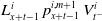 $L_{x+t-1}^{i}\, p_{x+t-1}^{i,m+1}\, V_{t^-}^i$
can be related to the expected mortality credits in such a state. Conversely,
$L_{x+t-1}^{i}\, p_{x+t-1}^{i,m+1}\, V_{t^-}^i$
can be related to the expected mortality credits in such a state. Conversely, $L_{x+t-1}^{i}\sum_{j\gt i}^m\, p_{x+t-1}^{i,j}$
is the number of individuals expected to move from state i to a living state
$L_{x+t-1}^{i}\sum_{j\gt i}^m\, p_{x+t-1}^{i,j}$
is the number of individuals expected to move from state i to a living state $j, j\gt i,$
and
$j, j\gt i,$
and $L_{x+t-1}^{i}\sum_{j\gt i} \,p_{x+t-1}^{i,j}\,\left(V_{t^-}^i-V_{t^-}^j\right)$
is a measure of the (total) net cross-subsidy ‘cost’ charged to state i for those expected to be alive, but in higher ageing states.
$L_{x+t-1}^{i}\sum_{j\gt i} \,p_{x+t-1}^{i,j}\,\left(V_{t^-}^i-V_{t^-}^j\right)$
is a measure of the (total) net cross-subsidy ‘cost’ charged to state i for those expected to be alive, but in higher ageing states.
The annual dynamics of the population of state i can be described for $t\gt0$
as follows:
$t\gt0$
as follows:
 \begin{equation} {} {} {} {}L_{x+t}^{i} = L_{x+t-1}^{i} + \sum_{j\lt i} L_{x+t-1}^{j,i} - \sum_{j\gt i}^{m+1} L_{x+t-1}^{i,j}, {}\end{equation}
where we use the notation $L_{x+t-1}^{j,i}$
(or
$L_{x+t-1}^{j,i}$
(or $L_{x+t-1}^{i,j}$
) to denote the observed number of individuals in state i (j) at time t being in state j (i) at time
$L_{x+t-1}^{i,j}$
) to denote the observed number of individuals in state i (j) at time t being in state j (i) at time $t-1$
. Equation (3.12) makes it clear that the number of individuals in state i at time t is the result of those who left state i (moving to a living state
$t-1$
. Equation (3.12) makes it clear that the number of individuals in state i at time t is the result of those who left state i (moving to a living state $j, \, i\lt j\leq m$
, or due to death,
$j, \, i\lt j\leq m$
, or due to death, $j=m+1$
) and those who have entered it from a state
$j=m+1$
) and those who have entered it from a state $j\lt i$
. Clearly,
$j\lt i$
. Clearly, $L_{x+t-1}^{j,i}=0$
for
$L_{x+t-1}^{j,i}=0$
for $i=1$
. Note that situations such as
$i=1$
. Note that situations such as $L_{x+t-1}^i=0$
and
$L_{x+t-1}^i=0$
and $L_{x+t}^i\gt0$
or
$L_{x+t}^i\gt0$
or $L_{x+t-1}^i\gt0$
and
$L_{x+t-1}^i\gt0$
and $L_{x+t}^i=0$
are possible, as a result of transitions into and out of state i. In the following, we use the notation
$L_{x+t}^i=0$
are possible, as a result of transitions into and out of state i. In the following, we use the notation $\widetilde{p}$
to denote the realised (observed) transition or permanence rates; for instance,
$\widetilde{p}$
to denote the realised (observed) transition or permanence rates; for instance, $\widetilde{p}_{x+t-1}^{\ i,j}=\frac{L_{x+t-1}^{i,j}}{L_{x+t-1}^{i}}$
. Such rates are obviously defined for states that are non-empty at time
$\widetilde{p}_{x+t-1}^{\ i,j}=\frac{L_{x+t-1}^{i,j}}{L_{x+t-1}^{i}}$
. Such rates are obviously defined for states that are non-empty at time $t-1$
, that is, for states i such that
$t-1$
, that is, for states i such that $L_{x+t-1}^{i}\gt0$
. Using this notation, Equation (3.12) can be rewritten as:
$L_{x+t-1}^{i}\gt0$
. Using this notation, Equation (3.12) can be rewritten as:
 \begin{equation} {} {}L_{x+t}^{i}= L_{x+t-1}^i \left(1-\widetilde{p}_{x+t-1}^{\ i,m+1}\right) +\sum_{j\lt i}L_{x+t-1}^{j}\, {}\widetilde{p}_{x+t-1}^{\ j,i}-\sum_{j\gt i}^{m}L_{x+t-1}^{i}\, \widetilde{p}_{x+t-1}^{\ i,j} . {}\end{equation}
Let us now compare $F_{t^-}^{i,A}$
to the pool fund required at time t for state i. As stated by (3.6), such a fund is proportional to
$F_{t^-}^{i,A}$
to the pool fund required at time t for state i. As stated by (3.6), such a fund is proportional to $L_{x+t}^{i} $
. Its amount before the adjustment of the benefits is represented by:
$L_{x+t}^{i} $
. Its amount before the adjustment of the benefits is represented by:
 \begin{equation} {} {}F_{t^-}^{i, R}=L_{x+t}^i\, V_{t^{-}}^i. {}\end{equation}
If we plug (3.13) into (3.14), we obtain the expression:
 \begin{equation} {} {}F_{t^-}^{i, R}= L_{x+t-1}^i \left(1-\widetilde{p}_{x+t-1}^{\ i,m+1}\right)\, V_{t^{-}}^i+\sum_{j\lt i}L_{x+t-1}^{j}\, \widetilde{p}_{x+t-1}^{\ j,i}\,V_{t^{-}}^{i}-\sum_{j\gt i}^{m}L_{x+t-1}^{i}\, \widetilde{p}_{x+t-1}^{\ i,j}\, V_{t^{-}}^{i}, {}\end{equation}
that we can compare with (3.11) for an interpretation. It is unlikely that $F_{t^-}^{i,A}=F_{t^-}^{i,R}$
, for a number of reasons:
$F_{t^-}^{i,A}=F_{t^-}^{i,R}$
, for a number of reasons:
-
• The realised number of deaths, $L_{x+t-1}^i\, \widetilde{p}_{x+t-1}^{\ i,m+1}$
, can be other than what expected,
$L_{x+t-1}^{i} \,p_{x+t-1}^{i,m+1}$
, and then the realised mortality credits in state i can be higher or lower than expected. We may consider it appropriate for any discrepancy to be absorbed by state i, given that this mismatch arises exclusively from mortality in state i.
$L_{x+t-1}^i\, \widetilde{p}_{x+t-1}^{\ i,m+1}$
, can be other than what expected,
$L_{x+t-1}^{i} \,p_{x+t-1}^{i,m+1}$
, and then the realised mortality credits in state i can be higher or lower than expected. We may consider it appropriate for any discrepancy to be absorbed by state i, given that this mismatch arises exclusively from mortality in state i. -
• In face of individuals entering state i during the year, it is required to hold in this state an additional amount
$\sum_{j\lt i}L_{x+t-1}^{j}\, \widetilde{p}_{x+t-1}^{\ j,i}\,V_{t^{-}}^{i}$
, which is not already included in
$F_{t^-}^{i,A}$
. This is an amount that should be cross-subsidised by the previous states
$j,j\lt i$
. -
• Individual funds
$V_{t^-}^j$
for those moving to a living state
$j,j\gt i$
are no longer required in state i and should be taken out from
$F_{t^-}^{i,A}$
, to cross-subsidise the next states. This is in line with what was discussed with regard to those entering state i (previous point). -
• Finally, we note that when
$L_{x+t}^i=0$
, then
$F_{t^-}^{i,R}=0$
; it can happen, instead, that
$F_{t^-}^{i,A}\gt0$
, given that this latter fund is assessed based on expected number of transitions, in contrast to
$F_{t^-}^{i,R}$
which considers realised transitions. In such a circumstance,
$F_{t^-}^{i,A}$
should be released to non-empty states.





Based on the above considerations, we define the pool fund available for state i at time t as follows:
 \begin{equation} {} {}F_{t}^{i, A}= \begin{cases} {} {} {}F_{t^-}^{i, A} +\displaystyle\sum_{j\lt i}L_{x+t-1}^{j}\, \widetilde{p}_{x+t-1}^{\ j,i}\,V_{t^{-}}^{i}-\sum_{j\gt i}^{m}L_{x+t-1}^{i}\, \widetilde{p}_{x+t-1}^{\ i,j}\, V_{t^{-}}^{j} +X_t^i & \text{if }L_{x+t}^i\gt0;\\ {} {} {}0 & \text{if }L_{x+t}^i=0. {} {}\end{cases} {}\end{equation}
With $X_t^i$
we denote the amount of resources left at time t by empty states, released to state i, so to ensure that
$X_t^i$
we denote the amount of resources left at time t by empty states, released to state i, so to ensure that $\sum_{i}F_t^{i, A}=F_t^A$
. We assume a redistribution proportional to the required funds before the adjustment of the benefits; more precisely, we assume (for non-empty states i):
$\sum_{i}F_t^{i, A}=F_t^A$
. We assume a redistribution proportional to the required funds before the adjustment of the benefits; more precisely, we assume (for non-empty states i):
 \begin{equation*} {} {}X_t^i=\left(F_t^A-\sum_{i:\,L^i_{x+t}\,\gt0} F_{t^-}^{i,A}\right)\,\frac{F_{t^-}^{i,R}}{F_{t^-}^R}. {}\end{equation*}
As already noted, definition (3.16) ensures $\sum_{i}F_t^{i,A}=F_t^A$
. The amounts
$\sum_{i}F_t^{i,A}=F_t^A$
. The amounts $\sum_{j\lt i}L_{x+t-1}^{j}\, \widetilde{p}_{x+t-1}^{\ j,i}\,V_{t^{-}}^{i}$
and
$\sum_{j\lt i}L_{x+t-1}^{j}\, \widetilde{p}_{x+t-1}^{\ j,i}\,V_{t^{-}}^{i}$
and $\sum_{j\gt i}^{m}L_{x+t-1}^{i}\, \widetilde{p}_{x+t-1}^{\ i,j}\, V_{t^{-}}^{j}$
measure the cross-subsidy, respectively, in favour of and released by state i. These amounts are also present in
$\sum_{j\gt i}^{m}L_{x+t-1}^{i}\, \widetilde{p}_{x+t-1}^{\ i,j}\, V_{t^{-}}^{j}$
measure the cross-subsidy, respectively, in favour of and released by state i. These amounts are also present in $F_t^A$
because, when we deal with multiple states, necessarily cross-subsidy effects between states are involved; however, such cross-subsidies are not explicit in (3.4) because they sum up to zero at the pool level.
$F_t^A$
because, when we deal with multiple states, necessarily cross-subsidy effects between states are involved; however, such cross-subsidies are not explicit in (3.4) because they sum up to zero at the pool level.
3.4 Adjustment of the benefits by state
Once the pool fund available for state i at time t, that is $F_t^{i, A}$
, is defined, we proceed to the adjustment of benefits imposing (3.7). We point out that this is a set of equations that must be solved backwards, from state m down to state 1. In particular, for
$F_t^{i, A}$
, is defined, we proceed to the adjustment of benefits imposing (3.7). We point out that this is a set of equations that must be solved backwards, from state m down to state 1. In particular, for $i=m$
, we have
$i=m$
, we have
 \begin{equation*} {} {} {}L_{x+t}^m B_{t}^m \ddot{a}_{x+t}^{m,m}=F_t^{m, A}, {} {}\end{equation*}
and the unknown $B_t^m$
straightforwardly follows:
$B_t^m$
straightforwardly follows:
 \begin{equation*} {} {} {}B_t^m=\frac{F_{t}^{m, A}}{L_{x+t}^{m}}\frac{1}{\ddot{a}^{m,m}_{x+t}}. {} {}\end{equation*}
For $i=m-1$
, by imposing
$i=m-1$
, by imposing
 \begin{equation*} {} {} {}L_{x+t}^m \left( B_{t}^{m-1} \ddot{a}_{x+t}^{m-1,m-1}+ B_{t}^m \ddot{a}_{x+t}^{m-1,m}\right)=F_t^{m-1, A} {} {}\end{equation*}
the unknown is $B_t^{m-1}$
, being
$B_t^{m-1}$
, being $B_t^{m}$
previously determined, and it holds that:
$B_t^{m}$
previously determined, and it holds that:
 \begin{equation*} {} {} {}B_t^{m-1}=\left(\frac{F_{t}^{m-1, A}}{L_{x+t}^{m-1}}-B_{t}^m \ddot{a}_{x+t}^{m-1,m}\right)\frac{1}{\ddot{a}^{m-1,m-1}_{x+t}}. {} {}\end{equation*}
Proceeding iteratively, for the non-empty states, we find
 \begin{equation} {} {} {}B_t^i=\left(\frac{F_{t}^{i, A}}{L_{x+t}^{i}}-\sum_{j\gt i}B_t^j\,{\ddot{a}^{i,j}_{x+t}} \right)\frac{1}{\ddot{a}^{i,j}_{x+t}}, {} {}\end{equation}
while we assume that if $L_{x+t}^i=0$
, then
$L_{x+t}^i=0$
, then $B_t^i=B_{t-1}^i$
(i.e., no adjustment is applied to benefits relating to empty states).
$B_t^i=B_{t-1}^i$
(i.e., no adjustment is applied to benefits relating to empty states).
An interesting interpretation of the adjustment can be found in terms of individual fund $V_t^i$
. For brevity, we develop it under the assumption
$V_t^i$
. For brevity, we develop it under the assumption $L_{x+t-1}^i\gt0$
and
$L_{x+t-1}^i\gt0$
and $X_t^i=0$
for all states i.
$X_t^i=0$
for all states i.
If we equate (3.6)–(3.16), and rearrange, we get
 \begin{equation} {} {}\begin{aligned} {} {} {}V_t^{i} \left(L_{x+t}^i-\sum_{j\lt i}L_{x+t-1}^{j}\, \widetilde{p}_{x+t-1}^{\ j,i}\right) & = L_{x+t-1}^{i}\,p_{x+t-1}^{i,i}\, V_{t^-}^{i}+ \sum_{j\lt i}L_{x+t-1}^{j}\, \widetilde{p}_{x+t-1}^{\ j,i}\,(V_{t^-}^{i}-V_{t}^{i})\\& \quad- L_{x+t-1}^{i}\sum_{j\gt i}^m\left(\widetilde{p}_{x+t-1}^{\ i,j}-p_{x+t-1}^{i,j}\right)\,V_{t^-}^j. {} {}\end{aligned} {}\end{equation}
Since (3.13) can also be written as
 \begin{equation*} {} {}L_{x+t}^i= L_{x+t-1}^{i}\, \widetilde{p}_{x+t-1}^{\ i,i}+\sum_{j\lt i}L_{x+t-1}^{j}\, \widetilde{p}_{x+t-1}^{\ j,i}, {}\end{equation*}
from (3.18) we obtain
 \begin{equation} {} {}V_t^{i} = \frac{p_{x+t-1}^{i,i}}{\widetilde{p}_{x+t-1}^{\, i,i}}\, V_{t^-}^{i}-\frac{\displaystyle\sum_{j\lt i}L_{x+t-1}^{j}\, \widetilde{p}_{x+t-1}^{\ j,i}}{L_{x+t-1}^{i}\, \widetilde{p}_{x+t-1}^{\ i,i}}\,(V_{t}^{i}-V_{t^-}^{i})-\frac{\displaystyle \sum_{j\gt i}^m\left(\widetilde{p}_{x+t-1}^{\, i,j}-p_{x+t-1}^{i,j}\right)}{\widetilde{p}_{x+t-1}^{\, i,i}}\, V_{t^{-}}^{j}. {}\end{equation}
When adjusting the benefits, clearly, we also need to adjust the individual required funds. Equation (3.19) suggests the following interpretation. The individual fund required at time t for state i must be adjusted because:
-
• The proportion of individuals remaining in state i differs from what was expected (see the first term of Equation (3.19));
-
• The cross-subsidy received for individuals entering state i from lower states
$j,j\lt i$
is based on
$V_{t^-}^i$
, but it must be updated to
$V_t^{i}$
after the adjustment (see the second term of Equation (3.19)); -
• The cross-subsidy transferred to higher states
$j,j\gt i$
is based on the realised transition rates, whereas the amount set aside in
$F_{t^-}^{i, A}$
is based on the expected transition rates (see the third term of Equation (3.19)).


We would like to emphasise that the first term recalls the mortality experience adjustment (MEA) factor introduced in Piggott et al. (Reference Piggott, Valdez and Detzel2005). It expresses the benefit update implied by the discrepancy between expected and realised mortality. In our multi-state framework, such an adjustment applies state-specific, accounting for ageing and mortality deviations. The second and third terms in Equation (3.19) correct the state-specific adjustment by accounting for, respectively, cross-subsidy inflows and outflows. Naturally, cross-subsidy cash flows can be defined in alternative ways; for instance, their amounts may be shaped based on the expected transition rates rather than realised values. Beyond the possible choices and consequent algebraic expressions, individual funds and benefits must be updated when experience differs from expectations, that is, realised cross-subsidies differ from those expected.
3.5 Smoothing benefits across states
The reasons that may lead an individual to prefer participation in a GSA scheme over the purchase of a life annuity are extensively discussed in the literature (see also Section 1); above all, cost savings, albeit at the expense of guarantees. When dealing with a multi-state GSA, one should additionally wonder why an individual should choose it, rather than one offering identical benefits across all states.
Similarly to a standard annuity, an individual who is aware of being in substandard health or maintaining unhealthy lifestyle patterns might feel disadvantaged by the use of undifferentiated annuity rates (see, e.g., Olivieri and Tabakova Reference Olivieri and Tabakova2024 for the case of annuities and Kabuche et al. Reference Kabuche, Sherris, Villegas and Ziveyi2024 for the case of a GSA). On the other hand, an individual currently in good health may feel better protected by a scheme that guarantees an upgrade in the benefit in the event of a deterioration in their health status. In this preference, one may recognise an interest akin to that observed for long-term care insurance products or disability income annuities.
Although GSA members are expected to accept benefit fluctuations across states depending on experience, they may reasonably expect a consistent and coherent ordering of those benefits, that is, $B_t^1\lt B_t^2\lt\ldots\lt B_t^m$
at all times
$B_t^1\lt B_t^2\lt\ldots\lt B_t^m$
at all times $t\geq0$
. At time
$t\geq0$
. At time $t=0$
, this is ensured by the initial choice of the benefit amounts; however, Equation (3.17) does not necessarily maintain such an ordering at later times (
$t=0$
, this is ensured by the initial choice of the benefit amounts; however, Equation (3.17) does not necessarily maintain such an ordering at later times ( $t\gt0$
), as it does not explicitly consider the relative differences among benefit levels. We also note that, even when the ordering of benefits is preserved, the distance between them may fall below desirable thresholds. These considerations suggest the introduction of corrective mechanisms to the adjustment rule described in Section 3.4.
$t\gt0$
), as it does not explicitly consider the relative differences among benefit levels. We also note that, even when the ordering of benefits is preserved, the distance between them may fall below desirable thresholds. These considerations suggest the introduction of corrective mechanisms to the adjustment rule described in Section 3.4.
There is a further circumstance that may require modifications to the adjustment rule. As we have discussed earlier (see Sections 1, 2 and 3.1), ageing states are usually not observable. The current mortality profile of an individual can reasonably be detected based on proxy risk factors, which may lead to a classification of individuals that does not precisely replicate the intended ageing states. Moreover, either by design or in connection with the available proxy risk factors, it could be considered more appropriate to structure benefits across $m^*$
classes, not necessarily matching the number of ageing states, that is,
$m^*$
classes, not necessarily matching the number of ageing states, that is, $m^*\leq m$
. In settings where m is large, adopting fewer benefit classes,
$m^*\leq m$
. In settings where m is large, adopting fewer benefit classes, $m^*\lt m$
, may offer a more practicable implementation. Illustrative proxy risk factors include medical events like the development of diabetes or a heart attack, as well as milder but indicative conditions such as hypertension, elevated glucose or cholesterol levels, or macular disease. They may also encompass functional or cognitive impairments, such as difficulties in performing activities of daily living or the onset of dementia. It should be noted that, given the absence of guarantees, the scheme may allow for a classification based on medical conditions or diseases that are typically excluded from standard insurance coverage. However, since more severe conditions result in access to a higher benefit class, safeguards must be anyhow in place to avoid potential misuse or fraud.
$m^*\lt m$
, may offer a more practicable implementation. Illustrative proxy risk factors include medical events like the development of diabetes or a heart attack, as well as milder but indicative conditions such as hypertension, elevated glucose or cholesterol levels, or macular disease. They may also encompass functional or cognitive impairments, such as difficulties in performing activities of daily living or the onset of dementia. It should be noted that, given the absence of guarantees, the scheme may allow for a classification based on medical conditions or diseases that are typically excluded from standard insurance coverage. However, since more severe conditions result in access to a higher benefit class, safeguards must be anyhow in place to avoid potential misuse or fraud.
In the following, we still refer to E as the set of ageing states and to $E^*=\{1,2,\ldots, m^*\}$
as the set of benefit classes. Benefits
$E^*=\{1,2,\ldots, m^*\}$
as the set of benefit classes. Benefits $B_t^i$
assessed as in Equation (3.17) ensure the actuarial equivalence between benefits and available resources by ageing state and for the whole pool, as discussed in Section 3.3. In the following, we refer to them as the notional benefits (or benefits by ageing state). We note that
$B_t^i$
assessed as in Equation (3.17) ensure the actuarial equivalence between benefits and available resources by ageing state and for the whole pool, as discussed in Section 3.3. In the following, we refer to them as the notional benefits (or benefits by ageing state). We note that
 \begin{equation} {} {}B_t^{TOT}=\sum_{i\in E} L_{x+t}^i\,B_t^i {}\end{equation}
measures the total payout admitted by the actuarial equivalence condition (3.7) at time $t,t\geq0$
. We denote with
$t,t\geq0$
. We denote with $\overline{B}_t^k$
the benefit for class
$\overline{B}_t^k$
the benefit for class $k\in E^*$
, and to keep the actuarial equivalence at the pool level, we require
$k\in E^*$
, and to keep the actuarial equivalence at the pool level, we require
 \begin{equation} {} {}\sum_{k\in E^*} l_{x+t}^k\,\overline{B}_t^k = B_t^{TOT} , {}\end{equation}
where $l_{x+t}^k$
is the number of survivors placed in benefit class k at time t (note that
$l_{x+t}^k$
is the number of survivors placed in benefit class k at time t (note that $\sum_{i\in E} L_{x+t}^i=\sum_{k\in E^*}l_{x+t}^k$
). We refer to
$\sum_{i\in E} L_{x+t}^i=\sum_{k\in E^*}l_{x+t}^k$
). We refer to $\overline{B}_t^k$
also as the actual benefits. Based on the motivations mentioned above, we introduce the further requirement:
$\overline{B}_t^k$
also as the actual benefits. Based on the motivations mentioned above, we introduce the further requirement:
 \begin{equation} {} {}\overline{B}_t^k = u^k\,\overline{B}_t^1 , {}\end{equation}
where $\overline{B}_t^1$
is the benefit amount for the lowest benefit class, and
$\overline{B}_t^1$
is the benefit amount for the lowest benefit class, and $u^k$
,
$u^k$
, $k=2,3,\ldots,m^*$
, is a coefficient chosen to achieve the desired differential between the benefit in class k and class 1. Reasonably,
$k=2,3,\ldots,m^*$
, is a coefficient chosen to achieve the desired differential between the benefit in class k and class 1. Reasonably, $1\lt u^2\lt u^3\lt\ldots \lt u^{m^*}$
. To avoid potential misunderstandings when comparing the coefficients
$1\lt u^2\lt u^3\lt\ldots \lt u^{m^*}$
. To avoid potential misunderstandings when comparing the coefficients $c^i$
’s introduced in Section 3.2 and the coefficients
$c^i$
’s introduced in Section 3.2 and the coefficients $u^k$
’s, we stress that, by design,
$u^k$
’s, we stress that, by design, $u^k$
measures the ratio at any time t between the actual benefit in class k in respect of class 1. The coefficient
$u^k$
measures the ratio at any time t between the actual benefit in class k in respect of class 1. The coefficient $c^i$
, instead, describes the initial level of differentiation across ageing-state benefits at time 0; at the following times
$c^i$
, instead, describes the initial level of differentiation across ageing-state benefits at time 0; at the following times $t,t=1,2,\ldots$
, it may turn out
$t,t=1,2,\ldots$
, it may turn out $B_t^i\gtreqless c^i B_t^1$
, as a result of the different benefit dynamics by ageing state. Based on (3.22), Equation (3.21) admits only one solution. After noting that requirement (3.22) introduces a kind of smoothing of benefits, we point out that benefits subjected to (3.22) bring us back to the solution discussed in Section 3.2 after Equation (3.5). Indeed, they may differ from that solution because of the number
$B_t^i\gtreqless c^i B_t^1$
, as a result of the different benefit dynamics by ageing state. Based on (3.22), Equation (3.21) admits only one solution. After noting that requirement (3.22) introduces a kind of smoothing of benefits, we point out that benefits subjected to (3.22) bring us back to the solution discussed in Section 3.2 after Equation (3.5). Indeed, they may differ from that solution because of the number $m^*$
of benefit classes (and the specific choice of the proportion among benefits), but basically, they follow the same idea. Yet, the analysis conducted in Sections 3.3 and 3.4 is not redundant, as it enables us to assess the extent of solidarity entailed by this choice.
$m^*$
of benefit classes (and the specific choice of the proportion among benefits), but basically, they follow the same idea. Yet, the analysis conducted in Sections 3.3 and 3.4 is not redundant, as it enables us to assess the extent of solidarity entailed by this choice.
As already noted, while actual benefits ensure actuarial equivalence at the pool level, the actuarial equivalence at the ageing state level will clearly be lost. This means that by adopting benefits $\overline{B}_t^k$
’s instead of
$\overline{B}_t^k$
’s instead of $B_t^i$
’s, solidarity mechanisms are introduced in the benefit design. With reference to an individual in ageing state i, placed in benefit class k, the size and direction of solidarity can be understood by comparing the actual benefit
$B_t^i$
’s, solidarity mechanisms are introduced in the benefit design. With reference to an individual in ageing state i, placed in benefit class k, the size and direction of solidarity can be understood by comparing the actual benefit $\overline{B}_t^k$
with the notional benefit
$\overline{B}_t^k$
with the notional benefit $B_t^i$
. Clearly, for some individuals
$B_t^i$
. Clearly, for some individuals $\overline{B}_t^k\lt B_t^i$
, meaning that they are contributing solidarity, whereas for others
$\overline{B}_t^k\lt B_t^i$
, meaning that they are contributing solidarity, whereas for others $\overline{B}_t^k\gt B_t^i$
, that is, they are receiving solidarity. We underline that this constitutes a design choice, albeit one that, in specific contexts, is imposed by the limited information available on individual mortality patterns. As pointed out in Section 1, understanding the solidarity effects introduced enables a rational justification and communication of design decisions, which is particularly important in arrangements where participants are exposed to the full range of shared risks. A numerical assessment is discussed in Section 4.2, which also clarifies why the introduction of solidarity effects may prove to be recommended.
$\overline{B}_t^k\gt B_t^i$
, that is, they are receiving solidarity. We underline that this constitutes a design choice, albeit one that, in specific contexts, is imposed by the limited information available on individual mortality patterns. As pointed out in Section 1, understanding the solidarity effects introduced enables a rational justification and communication of design decisions, which is particularly important in arrangements where participants are exposed to the full range of shared risks. A numerical assessment is discussed in Section 4.2, which also clarifies why the introduction of solidarity effects may prove to be recommended.
4. Numerical application
In the following, we delve into the proposed theoretical framework through a numerical application.
Mortality rates provided by the Human Mortality Database are used to fit the Markov ageing model, and different mortality experiences are selected to test the robustness of the fitting procedure. In particular, we refer to mortality rates of the 1920, 1930 and 1940 Australian cohorts, for both genders, considering ages 65 and above. We denote by $m_{x,c}$
the observed mortality rate at age x for the cohort c, with
$m_{x,c}$
the observed mortality rate at age x for the cohort c, with $c=1920,1930,1940$
. The age sets we deal with are
$c=1920,1930,1940$
. The age sets we deal with are $\mathcal{X}_{1920}=\{65,66, \ldots, 100\}$
,
$\mathcal{X}_{1920}=\{65,66, \ldots, 100\}$
, $\mathcal{X}_{1930}=\{65,66, \ldots, 90\}$
and
$\mathcal{X}_{1930}=\{65,66, \ldots, 90\}$
and $\mathcal{X}_{1940}=\{65,66, \ldots, 80\}$
for the 1920, 1930 and 1940 cohorts, respectively.
$\mathcal{X}_{1940}=\{65,66, \ldots, 80\}$
for the 1920, 1930 and 1940 cohorts, respectively.
In Section 4.1, the procedure adopted for fitting the Markov ageing model will be discussed, as well as the strategy employed to simulate transitions between the process’s states. The numerical implementation of the Markov ageing GSA will be exposed in Section 4.2. For the sake of conciseness, some numerical results are collected in the Supplementary Material accompanying the present manuscript.
4.1 Model fitting and simulation
To fit the Markov ageing model, both the initial distribution $\boldsymbol{\pi}$
and the intensity matrix
$\boldsymbol{\pi}$
and the intensity matrix $\boldsymbol{\Lambda}$
of the ageing process must be estimated, and the choice of fitting method may be affected by the data availability. At first glance, the maximum-likelihood estimation (MLE) approach represents a natural candidate for fitting the Markov ageing model. To perform the MLE procedure, independent trajectories of the ageing process must be completely observed up to the time of death. Each path should consist of the sequence
$\boldsymbol{\Lambda}$
of the ageing process must be estimated, and the choice of fitting method may be affected by the data availability. At first glance, the maximum-likelihood estimation (MLE) approach represents a natural candidate for fitting the Markov ageing model. To perform the MLE procedure, independent trajectories of the ageing process must be completely observed up to the time of death. Each path should consist of the sequence $\left\{\left(i_k,s_k\right), \, k=1,2,\ldots,n\right\}$
, where
$\left\{\left(i_k,s_k\right), \, k=1,2,\ldots,n\right\}$
, where $i_1,i_2,\ldots, i_n$
are the ageing states visited before death, and
$i_1,i_2,\ldots, i_n$
are the ageing states visited before death, and $s_1,s_2,\ldots,s_n$
are the corresponding sojourn times. However, due to the latent nature of the ageing states, trajectories of the ageing process are not detectable, and the likelihood function maximisation cannot be directly executed. Nonetheless, if realisations of i.i.d. times until death are accessible, the MLE can be carried out via the expectation-maximisation (EM) algorithm. Assuming that an underlying ageing process generates such absorption times, the conditional expected value of the log-likelihood function can be computed and then maximised w.r.t. model parameters. In case no information on the times until death is available, they could be randomly drawn from a valid PH distribution. The simulation exercise requires that several combinations of the initial probability vector and the intensity matrix must be tried, as well as different numbers of EM iterations should be considered. It could be computationally expensive, and there is no guarantee that the maximum of the likelihood function is achieved. Indeed, while the EM algorithm always converges, it does not necessarily converge to the ML estimator as it can be trapped in a local maximum. The EM algorithm can be exploited to its full effectiveness, for instance, when survival data are observable; however, this is not the case for the present analysis because only cohort mortality rates are available to us.
$s_1,s_2,\ldots,s_n$
are the corresponding sojourn times. However, due to the latent nature of the ageing states, trajectories of the ageing process are not detectable, and the likelihood function maximisation cannot be directly executed. Nonetheless, if realisations of i.i.d. times until death are accessible, the MLE can be carried out via the expectation-maximisation (EM) algorithm. Assuming that an underlying ageing process generates such absorption times, the conditional expected value of the log-likelihood function can be computed and then maximised w.r.t. model parameters. In case no information on the times until death is available, they could be randomly drawn from a valid PH distribution. The simulation exercise requires that several combinations of the initial probability vector and the intensity matrix must be tried, as well as different numbers of EM iterations should be considered. It could be computationally expensive, and there is no guarantee that the maximum of the likelihood function is achieved. Indeed, while the EM algorithm always converges, it does not necessarily converge to the ML estimator as it can be trapped in a local maximum. The EM algorithm can be exploited to its full effectiveness, for instance, when survival data are observable; however, this is not the case for the present analysis because only cohort mortality rates are available to us.
Given the above considerations, we opt for an alternative fitting method to MLE. For the sake of completeness, we refer the reader to the Section 1 of the Supplementary Material, where technical details on the EM-based fitting of the Markov ageing model are provided.
We proceed to fit the Markov ageing model by adopting a target approach, that is, a general procedure allowing for dealing directly with the observed mortality or survival curve. Let $\boldsymbol{\theta}_{c}=(\boldsymbol{\pi}_{c},\boldsymbol{\Lambda}_{c})$
be the parameter characterising the Markov ageing model for the cohort c. For each cohort, the deviations between the observed mortality data (the target) and the corresponding value provided by the ageing model are measured through a proper loss function
$\boldsymbol{\theta}_{c}=(\boldsymbol{\pi}_{c},\boldsymbol{\Lambda}_{c})$
be the parameter characterising the Markov ageing model for the cohort c. For each cohort, the deviations between the observed mortality data (the target) and the corresponding value provided by the ageing model are measured through a proper loss function $\mathcal{L}$
. We choose the mean squared error as the loss function, while our target is the t-year survival probability at age 65. Then, we have
$\mathcal{L}$
. We choose the mean squared error as the loss function, while our target is the t-year survival probability at age 65. Then, we have
 \begin{equation} {} {} {} {} {} {}\mathcal{L}(\boldsymbol{\theta}_c) = \dfrac{1}{\left\vert \mathcal{X}_{c} \right\vert} \sum_{t=1}^{\left\vert \mathcal{X}_{c} \right\vert} \left({}_t p_{65,c}-S_{65}\left(t;\;\boldsymbol{\theta}_{c}\right)\right)^2, {} {}\end{equation}
where ${}_t p_{65,c}$
is the t-year survival probability at age 65 for the cohort c and computed as
${}_t p_{65,c}$
is the t-year survival probability at age 65 for the cohort c and computed as ${}_t p_{65,c} = \prod_{h=0}^{t-1} \left(1-\frac{m_{65+h, c}}{1+0.5 \,m_{65+h, c}}\right)$
, while
${}_t p_{65,c} = \prod_{h=0}^{t-1} \left(1-\frac{m_{65+h, c}}{1+0.5 \,m_{65+h, c}}\right)$
, while $S_{65}\left(t;\;\boldsymbol{\theta}_{c}\right)$
is the survival function for the same cohort and its expression is given in Equation (2.7). We find the estimate
$S_{65}\left(t;\;\boldsymbol{\theta}_{c}\right)$
is the survival function for the same cohort and its expression is given in Equation (2.7). We find the estimate $\hat{\boldsymbol{\theta}}_{c}$
as the solution of the following constrained mean squared error minimisation problem:
$\hat{\boldsymbol{\theta}}_{c}$
as the solution of the following constrained mean squared error minimisation problem:
 \begin{equation} {} {} {} {} {} {}\min_{\boldsymbol{\theta}_{c}}\mathcal{L}(\boldsymbol{\theta}_c), \quad \text{s.t.} \quad \pi_{i, c} \in [0,1] \ \forall \, i \in E, \ \sum_{i \in E} \pi_{i, c} = 1, {} {}\end{equation}
which we solve numerically for each cohort and gender.
As mentioned in Section 2, two other aspects deserve consideration in fitting the Markov ageing model: the number of ageing phases, m, and possible non-uniqueness problems in parameter specifications. Concerning the latter, along the lines of Su and Sherris (Reference Su and Sherris2012), we impose the following specification for intensity matrix elements in (2.3):
 \begin{equation} {} {} {} {} {} {}\lambda_i = \lambda \quad \text{and} \quad q_i = \gamma + \alpha\,\text{e}^{\beta \, i}, \quad \forall \, i \in E, \, \gamma, \alpha, \beta \gt0. {} {}\end{equation}
A constant transition intensity between states means that, on average, a linear decline of various physiological functions is acknowledged. The transition towards the death state accounts for a background rate, namely $\gamma$
, and an ageing-dependent component,
$\gamma$
, and an ageing-dependent component, $\alpha\,\text{e}^{\beta \, i}$
. The former allows for the representation of ageing termination due to accidental death, while the latter describes an exponential increase in mortality as ageing proceeds. Regarding the number of ageing phases, an accurate fit of the entire mortality schedule could be attained for high values of m (see, e.g., Lin and Liu Reference Lin and Liu2007; Cheng et al. Reference Cheng, Jones, Liu and Ren2020); however, if only part of the mortality schedule is of interest, a low-dimensional PH distribution furnishes a satisfactory fit (see, e.g., Liu and Lin Reference Liu and Lin2012). Therefore, we select the number of phases empirically, starting with low m values and increasing them until the loss function reduces. In Table 2, mean squared error values are reported for different numbers of ageing phases, distinguishing by cohorts and genders. For the 1920 and 1930 Australian cohorts, we find that
$\alpha\,\text{e}^{\beta \, i}$
. The former allows for the representation of ageing termination due to accidental death, while the latter describes an exponential increase in mortality as ageing proceeds. Regarding the number of ageing phases, an accurate fit of the entire mortality schedule could be attained for high values of m (see, e.g., Lin and Liu Reference Lin and Liu2007; Cheng et al. Reference Cheng, Jones, Liu and Ren2020); however, if only part of the mortality schedule is of interest, a low-dimensional PH distribution furnishes a satisfactory fit (see, e.g., Liu and Lin Reference Liu and Lin2012). Therefore, we select the number of phases empirically, starting with low m values and increasing them until the loss function reduces. In Table 2, mean squared error values are reported for different numbers of ageing phases, distinguishing by cohorts and genders. For the 1920 and 1930 Australian cohorts, we find that $m=15$
ageing phases grant the best model fitting, for both genders; the same occurs for the 1940 cohorts with
$m=15$
ageing phases grant the best model fitting, for both genders; the same occurs for the 1940 cohorts with $m=7$
ageing phases. Figure 2 furnishes a graphical visualisation for the comparison between the observed t-years survival probabilities and the corresponding fitted values of the PH’s survival function. The latter are determined according to the m value providing the lowest mean squared error for each cohort and gender. We observe a satisfactory fit across all cohorts and both genders. The greater fitting accuracy is achieved for the younger cohorts, since their survival curve consists of a few observations outlining a non-complex trend over time.
$m=7$
ageing phases. Figure 2 furnishes a graphical visualisation for the comparison between the observed t-years survival probabilities and the corresponding fitted values of the PH’s survival function. The latter are determined according to the m value providing the lowest mean squared error for each cohort and gender. We observe a satisfactory fit across all cohorts and both genders. The greater fitting accuracy is achieved for the younger cohorts, since their survival curve consists of a few observations outlining a non-complex trend over time.
Mean squared error values by increasing the number of ageing phases, m, and distinguishing by cohorts and genders. The lowest mean squared error values are in bold.

Comparison between the observed t-years survival probabilities (red dots) and the corresponding fitted values of the PH’s survival function (blue triangles). The latter are determined according to the m value providing the lowest mean squared error for each cohort and gender (see Table 2).

For the sake of simplicity, from now on, we focus on the 5-state Markov ageing model for the 1920 Australian cohort, considering both genders. Using a low-dimensional Markov ageing model facilitates the readability of both the estimated parameters and the results of the Markov ageing GSA presented in Section 4.2. Comments we draw in the following discussions can be easily extended to high-dimensional Markov ageing models, as well as to the other cohorts. We refer the reader to Section 2 of the Supplementary Material for the parameters estimate concerning the befitting Markov ageing models.
Table 3 collects the 5-state Markov ageing mode’s parameters estimate concerning the 1920 Australian cohort. We note that, for both genders, the initial distribution of the process is mainly concentrated in the first ageing state, and it is residually located in the other states, in particular the last one. Then, 65-year-old individuals cannot be attributed to a unique ageing status; individuals differ in physiological state, even though they have the same chronological age. For the male gender, the probability of being in the first ageing state is lower than for the female gender; the opposite occurs if we consider the fifth state. Therefore, the physiological status of females chronologically aged 65 should be better than that of males. Such evidence is accompanied by the gender-based estimates of $\lambda$
. Females present a
$\lambda$
. Females present a $\lambda$
value lower than that for males, indicating a slower decline in their physiological functions. Considering the parameters embedded in the transition intensity to the death state, the background rate estimate appears negligible for both genders. Indeed, the background rate
$\lambda$
value lower than that for males, indicating a slower decline in their physiological functions. Considering the parameters embedded in the transition intensity to the death state, the background rate estimate appears negligible for both genders. Indeed, the background rate $\gamma$
measures the effects of accidental deaths, which mainly occur at adult ages, while we are referring to older ages. The
$\gamma$
measures the effects of accidental deaths, which mainly occur at adult ages, while we are referring to older ages. The $\beta$
parameter represents the rate at which the transition intensity to the death state varies as the ageing phases progress. The larger the value of
$\beta$
parameter represents the rate at which the transition intensity to the death state varies as the ageing phases progress. The larger the value of $\beta$
, the more likely the transition to the death state will be. As shown in Table 3, the female gender has a higher
$\beta$
, the more likely the transition to the death state will be. As shown in Table 3, the female gender has a higher $\beta$
than that for the male gender, but at the same time, there is a compensation with the respective
$\beta$
than that for the male gender, but at the same time, there is a compensation with the respective $\alpha$
parameter values. On the whole, we find that the female gender tends to experience a slower ageing process and a longer lifespan, compared to the male gender.
$\alpha$
parameter values. On the whole, we find that the female gender tends to experience a slower ageing process and a longer lifespan, compared to the male gender.
Estimate of the 5-state Markov ageing model’s parameters for the 1920 Australian cohort, both genders. We recall that: $\alpha$
is an ageing-related scale parameter,
$\alpha$
is an ageing-related scale parameter, $\beta$
denotes the rate of change of
$\beta$
denotes the rate of change of $q_i$
as ageing progresses,
$q_i$
as ageing progresses, $\gamma$
is the rate measuring the ageing termination due to accidental deaths,
$\gamma$
is the rate measuring the ageing termination due to accidental deaths, $\lambda$
is the transition intensity among states, and
$\lambda$
is the transition intensity among states, and $\pi_i$
is the probability that the process starts in the state i, for
$\pi_i$
is the probability that the process starts in the state i, for $i=1,\ldots, 5$
.
$i=1,\ldots, 5$
.

Following the model fitting, the evolution over time and by state of the initial population can be simulated. Similarly to Kabuche et al. (Reference Kabuche, Sherris, Villegas and Ziveyi2024), the realised number of individuals transitioning from state i to state j in the interval $(t-1,t]$
is randomly drawn from a multinomial distribution, that is,
$(t-1,t]$
is randomly drawn from a multinomial distribution, that is,
 \begin{equation} {} {} {} {}L_{x+t-1}^{i,j} \sim \text{Multinom}\left(L_{x+t-1}^i,p_{x+t-1}^{i,j}\right), \quad i \in E,\, j \in \mathcal{S}. {}\end{equation}
In (4.4), $L_{x+t-1}^i$
refers to the actual number of individuals belonging to the ageing state i at time
$L_{x+t-1}^i$
refers to the actual number of individuals belonging to the ageing state i at time $t-1$
, while
$t-1$
, while $p_{x+t-1}^{i,j}$
is the expected 1-year transition probability, from state i to state j, stemming from the calibrated Markov ageing model. At each time step, we run 10,000 simulations to generate population transitions among states. The total number of individuals attaining state j at time t is used for generating population transitions at time
$p_{x+t-1}^{i,j}$
is the expected 1-year transition probability, from state i to state j, stemming from the calibrated Markov ageing model. At each time step, we run 10,000 simulations to generate population transitions among states. The total number of individuals attaining state j at time t is used for generating population transitions at time $t+1$
. In addition, for each random draw, the simulated number
$t+1$
. In addition, for each random draw, the simulated number $L_{x+t-1}^{i,j}$
is used to compute the realised 1-year transition probabilities as
$L_{x+t-1}^{i,j}$
is used to compute the realised 1-year transition probabilities as $\widetilde{p}_{x+t-1}^{\, i,j}=\frac{L_{x+t-1}^{i,j}}{L_{x+t-1}^i}$
.
$\widetilde{p}_{x+t-1}^{\, i,j}=\frac{L_{x+t-1}^{i,j}}{L_{x+t-1}^i}$
.
4.2 Implementation of the Markov ageing GSA
4.2.1 Pool composition and population dynamics
We assume that at time $t=0$
the GSA scheme is joined by a cohort of
$t=0$
the GSA scheme is joined by a cohort of $L_x=10,000$
individuals (either females or males), chronological age
$L_x=10,000$
individuals (either females or males), chronological age $x=65$
; we further assume that the scheme closes upon reaching time
$x=65$
; we further assume that the scheme closes upon reaching time $t_{\max}=30$
. Consistent with the Markov ageing model calibrated as described in Section 4.1, individuals are distributed in five ageing states, with initial composition as in Table 4. We point out that such a composition (for both genders) naturally follows from the estimated initial distribution of the Markov process; see Table 3.
$t_{\max}=30$
. Consistent with the Markov ageing model calibrated as described in Section 4.1, individuals are distributed in five ageing states, with initial composition as in Table 4. We point out that such a composition (for both genders) naturally follows from the estimated initial distribution of the Markov process; see Table 3.
Initial pool composition, by gender.

Figure 3 plots the average number of survivors in the five ageing states across time, separately for females and males; this way, we have a representation of the population dynamics. The average paths of the five ageing states are similar for both genders: the decreasing pattern of state 1 is explained by the fact that individuals can only exit this state (either by jumping to a higher living state or because of death). The non-monotonic trajectories of the other states are driven by the net balance of transitions in and out of each state. States representing higher ageing levels reach their maximum size later than the others, and the peak population tends to decrease with increasing state severity. Nevertheless, at older chronological ages, and especially at the final time $t_{\max}$
, the higher ageing states are larger than the lower ones. In particular, state 1 exhibits a population size that almost disappears at later times, although for both genders, it does not die out by time
$t_{\max}$
, the higher ageing states are larger than the lower ones. In particular, state 1 exhibits a population size that almost disappears at later times, although for both genders, it does not die out by time $t_{\max}$
. When comparing these patterns between females and males, the greater average longevity of the former results in higher average sizes of the lower-index ageing states for females, at any given time.
$t_{\max}$
. When comparing these patterns between females and males, the greater average longevity of the former results in higher average sizes of the lower-index ageing states for females, at any given time.
Population dynamics (average value) by time (annual basis) and state for both genders. We refer the reader to the Section 3 of the Supplementary Material for the graphical representation of the population transitions among states, for both genders.

4.2.2 Available pool fund by state
The GSA scheme pays annual benefits to survivors at the beginning of the year, from time $t=0$
until time
$t=0$
until time $t_{\max}=30$
. We set
$t_{\max}=30$
. We set $B_0^1=1.00$
account unit and
$B_0^1=1.00$
account unit and $B_0^i=1.2^{i-1}\,B_0^1$
; Table 5 lists the initial benefit amounts by ageing state and the corresponding initial capital, assessed according to Equation (3.1). The discount rate is set to
$B_0^i=1.2^{i-1}\,B_0^1$
; Table 5 lists the initial benefit amounts by ageing state and the corresponding initial capital, assessed according to Equation (3.1). The discount rate is set to $r=0.02$
. For each gender, the higher initial capital required from members in ageing state 1 reflects their longer life expectancy, notwithstanding their lower initial benefit. Similarly, for a given state, higher initial capitals are charged to females as a consequence of their higher expected lifetime.
$r=0.02$
. For each gender, the higher initial capital required from members in ageing state 1 reflects their longer life expectancy, notwithstanding their lower initial benefit. Similarly, for a given state, higher initial capitals are charged to females as a consequence of their higher expected lifetime.
Initial notional benefit amount and capital, by gender.

Figure 4 shows the time profile of the average values of the pool fund available by state for females. The time profiles for males are similar and, for brevity, are not shown here, but they can be found in the Section 3 of the Supplementary Material.
Available fund (average value), and its components, by time (annual basis) and state for the female gender. y-axis values are on $10^{-4}$
scale. Since the fund value ranges differ significantly across the various states, we adopted separate y-axis scales to enhance the readability of the fund patterns for states
$10^{-4}$
scale. Since the fund value ranges differ significantly across the various states, we adopted separate y-axis scales to enhance the readability of the fund patterns for states $i \gt 1$
. For the male gender, refer to the Section 3 of the Supplementary Material.
$i \gt 1$
. For the male gender, refer to the Section 3 of the Supplementary Material.

The time profiles can be interpreted, in particular, considering the several components of the available pool fund by state, as defined in Equation (3.16). For each state, these components are included in the picture. In this regard, we point out that all quantities are plotted in absolute value; however, cross-subsidies may be either incoming or outgoing, depending on the states j considered in relation to state i.
In general, the time profile of each $F_t^{i, A}$
resembles that of survivors in the ageing state, that is,
$F_t^{i, A}$
resembles that of survivors in the ageing state, that is, $L_{65+t}^i$
, apart from scaling factors due to the benefit amounts. As the population ages, resources are shifted towards the more severe ageing states. In particular, cross-subsidy is prevalent between consecutive states. For instance, ageing state 2 receives people from state 1 increasing its heap of individual funds, that is,
$L_{65+t}^i$
, apart from scaling factors due to the benefit amounts. As the population ages, resources are shifted towards the more severe ageing states. In particular, cross-subsidy is prevalent between consecutive states. For instance, ageing state 2 receives people from state 1 increasing its heap of individual funds, that is, $L_{65+t}^{1,2}V_{t^-}^2$
, and transfers part of its individuals (and the relative funds) primarily to state 3, that is,
$L_{65+t}^{1,2}V_{t^-}^2$
, and transfers part of its individuals (and the relative funds) primarily to state 3, that is, $L_{65+t}^{2,3}V_{t^-}^3$
. In turn, ageing state 3 acquires people and funds from state 2, and part of its population is mainly relocated to ageing state 4, and so on. Both cross-subsidy inflows and outflows by state are reported in Table 6. It is worth noting that the cross-subsidy obtained by state 1 is null for every
$L_{65+t}^{2,3}V_{t^-}^3$
. In turn, ageing state 3 acquires people and funds from state 2, and part of its population is mainly relocated to ageing state 4, and so on. Both cross-subsidy inflows and outflows by state are reported in Table 6. It is worth noting that the cross-subsidy obtained by state 1 is null for every $t\gt0$
, as is the cross-subsidy offered by state 5. Since only forward ageing transitions are allowed in the Markov ageing model, the lowest ageing state subsidises all the next ones; conversely, the highest ageing state solely receives from the others. Given the initial population composition (see Table 4), the ageing state 1 brings individuals and related funds to subsequent states during the first year. Its cross-subsidy outflow at
$t\gt0$
, as is the cross-subsidy offered by state 5. Since only forward ageing transitions are allowed in the Markov ageing model, the lowest ageing state subsidises all the next ones; conversely, the highest ageing state solely receives from the others. Given the initial population composition (see Table 4), the ageing state 1 brings individuals and related funds to subsequent states during the first year. Its cross-subsidy outflow at $t=1$
is fully allocated among states
$t=1$
is fully allocated among states $j\gt1$
, corresponding to their respective inflows. As individuals age (or die), state 1 tends to empty, and fewer funds will be transferred. Meanwhile, ageing states
$j\gt1$
, corresponding to their respective inflows. As individuals age (or die), state 1 tends to empty, and fewer funds will be transferred. Meanwhile, ageing states $j\gt1$
experience an initial increase in incoming cross-subsidies, which then gives way to greater outflows as ageing progresses.
$j\gt1$
experience an initial increase in incoming cross-subsidies, which then gives way to greater outflows as ageing progresses.
Ingoing and outgoing cross-subsidies (average value) by state. Values refer to the female gender and, for conciseness, are reported for selected years. Note that, by means of Equation (3.16), the ingoing cross-subsidy for the state i at time $t\gt0$
is given by
$t\gt0$
is given by $\sum_{j\lt i}L_{x+t-1}^{j}\, \widetilde{p}_{x+t-1}^{\ j,i}\,V_{t^{-}}^{i}+X_t^i$
, while the outgoing cross-subsidy is quantified as
$\sum_{j\lt i}L_{x+t-1}^{j}\, \widetilde{p}_{x+t-1}^{\ j,i}\,V_{t^{-}}^{i}+X_t^i$
, while the outgoing cross-subsidy is quantified as $\sum_{j\gt i}^{m}L_{x+t-1}^{i}\, \widetilde{p}_{x+t-1}^{\ i,j}\, V_{t^{-}}^{j}$
. For the male gender, we refer the reader to the Section 3 of the Supplementary Material.
$\sum_{j\gt i}^{m}L_{x+t-1}^{i}\, \widetilde{p}_{x+t-1}^{\ i,j}\, V_{t^{-}}^{j}$
. For the male gender, we refer the reader to the Section 3 of the Supplementary Material.

Finally, we notice that $X_t^i$
is null over time and for all states. Such a result arises from state populations never becoming extinct; therefore, no state leaves resources to other states due to population depletion.
$X_t^i$
is null over time and for all states. Such a result arises from state populations never becoming extinct; therefore, no state leaves resources to other states due to population depletion.
4.2.3 Notional benefits
Figure 5 plots the time profile of the average value of the notional benefits by gender. For all states, benefits on average are quite stable; however, at higher chronological ages, they show either an increasing or decreasing path. Such a behaviour can be interpreted in view of cross-subsidy flows, arising from deaths, entries into the state and transitions to higher living states. We note, in particular, an increasing trend in state 5 (which can be exited only upon death) and a decreasing trend for the other states (which are likely to become thinnier, as a result of deaths and ageing). The effect of cross-subsidies for the various states can also be understood in light of the dynamics of the available pool funds by state (see Figure 4). We note that the male population in state 1 is the one that shrinks the most (due to deaths and ageing), see Figure 3; then, the average time profile of benefits in state 1 for males may suggest that cross-subsidies rooted in actuarial equivalence lead to undesirable benefit patterns when the number of participants becomes very low.
Individual notional benefits (average value) by time (annual basis) and ageing state, for both genders. For each ageing state, the black dashed line represents the initial benefit level, that is, $B_0^i$
for
$B_0^i$
for $i=1,\ldots,5$
, outlined in Table 5.
$i=1,\ldots,5$
, outlined in Table 5.

Indeed, the benefit dynamics in ageing state 1 deserves careful consideration. While it is true that individuals in this state are exposed to the risk of jumping to a higher state (where they would receive a higher benefit amount), it is also the case that those who remain in state 1 often do so as a result of healthier lifestyles and well-being-oriented behaviours (that may also prove to be more expensive than more passive, sedentary or unhealthy lifestyles). A reduction in benefits for state 1 (especially when, at the same time, benefits in the other states are increasing) may be perceived as a form of penalisation and a disincentive for behaviours that should instead be encouraged due to their social value. This is one of the reasons why it may be appropriate to introduce an adjustment to actuarially equivalent cross-subsidies, by admitting some kind of solidarity among states (see Section 3.5). Numerical results, in particular, suggest that the introduction of solidarity should be considered in favour of those in ageing state 1, that is, individuals with longer life expectancy, who spend their lives in better ageing conditions. This conclusion may appear counterintuitive, as we are naturally inclined to believe that financial support should be directed from healthier individuals to those in poorer health. Thanks to our modelling framework, we are able to gain deeper insight into this issue, so as to enable more informed decision-making with respect to the GSA design.
4.2.4 Actual benefits
Notional benefits can be repackaged into actual benefits in a number of ways, each of which implies some degree of solidarity that individuals may perceive as either acceptable or not. For instance, if we consider a plain GSA, that is, a scheme with undifferentiated benefits, it is not difficult to conclude from Figure 5 that the common benefit amount falls between the lowest and the highest notional benefit amounts. Individuals in lower ageing states would implicitly receive solidarity from those in higher ageing states. The difference between notional and actual benefits in this case can be significant enough to lead certain categories of people to opt out of the scheme (provided that participation is not mandatory).
We examine numerically some benefit smoothing solutions that may be seen as suitable by various population groups. We consider four cases:
-
•
$m^*=1$
, meaning that a unique benefit class is acknowledged. In other words, we look at a plain GSA wherein all the ageing states are grouped since the scheme provides undifferentiated benefits; -
•
$m^*=2$
, that is, two classes of benefit, assuming that
$u^2=1.5$
,
$l_{x+t}^1 = L_{x+t}^1 + L_{x+t}^2$
and
$l_{x+t}^2 = L_{x+t}^3 + L_{x+t}^4 + L_{x+t}^5$
. This way, ageing states 1 and 2, on the one side, and ageing states 3, 4, and 5, on the other, are grouped. These groupings are based on the assumption that individuals in adjacent ageing states are unlikely to clearly distinguish between their respective mortality characteristics; -
•
$m^*=3$
, that is, three classes of benefit, assuming that
$u^2=1.5$
,
$u^3=2$
,
$l_{x+t}^1 = L_{x+t}^1 + L_{x+t}^2$
,
$l_{x+t}^2 = L_{x+t}^3 + L_{x+t}^4$
and
$l_{x+t}^3 = L_{x+t}^5$
. In this case, ageing class 5 is kept by itself; -
•
$m^*=5$
, that is, five classes of benefit, assuming that
$u^2=1.25$
,
$u^3=1.5$
,
$u^4=1.75$
,
$u^5=2$
and
$l_{x+t}^k = L_{x+t}^i$
for every
$k,i =1,\ldots,5$
, with
$k=i$
. We point out that this case corresponds to the solution described in Section 3.2, after Equation (3.5).









The numerical results are plotted in Figure 6, for females (for males, see Section 3 of the Supplementary Material). The smoothing effect is apparent in all cases (as it can be easily seen when comparing Figure 5 with Figure 6); in particular, as a consequence of the imposed linking among the various benefit classes, the benefit trajectory is identical across all classes, apart from the chosen scaling factor. It should be noted that, in any case, the total payout of the pool remains the same (i.e., $B_t^{TOT}$
) at all times and is determined by requiring funded liabilities by ageing state (i.e., imposing (3.7)). Solidarity contributions can be understood by comparing the notional with the actual benefit for each ageing state. In Table 7, both notional and actual benefits are presented by considering different numbers of benefit classes. In general, higher ageing states offer solidarity to lower ones. The size of such contributions depends on the specific choice of the benefit classes and the chosen proportions among benefit amounts. For instance, if a unique benefit class is acknowledged (i.e.,
$B_t^{TOT}$
) at all times and is determined by requiring funded liabilities by ageing state (i.e., imposing (3.7)). Solidarity contributions can be understood by comparing the notional with the actual benefit for each ageing state. In Table 7, both notional and actual benefits are presented by considering different numbers of benefit classes. In general, higher ageing states offer solidarity to lower ones. The size of such contributions depends on the specific choice of the benefit classes and the chosen proportions among benefit amounts. For instance, if a unique benefit class is acknowledged (i.e., $m^\star=1$
), then lower ageing states receive solidarity from higher ageing states along the entire scheme duration. In particular, it holds that
$m^\star=1$
), then lower ageing states receive solidarity from higher ageing states along the entire scheme duration. In particular, it holds that $B_t^i\lt\overline{B}_t^1$
, for
$B_t^i\lt\overline{B}_t^1$
, for $i=1,2$
and for every
$i=1,2$
and for every $t\gt0$
, while ageing states 3 and 4 offer solidarity, respectively, until the end of the 10th and 25th year. State 5, instead, only contributes to solidarity each year. Now, let us consider
$t\gt0$
, while ageing states 3 and 4 offer solidarity, respectively, until the end of the 10th and 25th year. State 5, instead, only contributes to solidarity each year. Now, let us consider $m^\star=2$
benefit classes. We recall that individuals belonging to the first and second ageing states, that is,
$m^\star=2$
benefit classes. We recall that individuals belonging to the first and second ageing states, that is, $L_{x+t}^1$
and
$L_{x+t}^1$
and $L_{x+t}^2$
, are relocated into the first benefit class since
$L_{x+t}^2$
, are relocated into the first benefit class since $l_{x+t}^1= L_{x+t}^1+L_{x+t}^2$
. As emerges in Table 7, individuals in the first ageing state will earn solidarity, being
$l_{x+t}^1= L_{x+t}^1+L_{x+t}^2$
. As emerges in Table 7, individuals in the first ageing state will earn solidarity, being $B_t^i\lt\overline{B}_t^1$
for every
$B_t^i\lt\overline{B}_t^1$
for every $t\gt0$
; conversely, individuals in the ageing state 2 obtain an actual benefit lower than the corresponding notional ones until the twentieth year. The second benefit class pays the actual benefits
$t\gt0$
; conversely, individuals in the ageing state 2 obtain an actual benefit lower than the corresponding notional ones until the twentieth year. The second benefit class pays the actual benefits $\overline{B}_t^2$
to individuals residing in the states 3, 4 and 5. Comparing the actual benefits with the notional benefits
$\overline{B}_t^2$
to individuals residing in the states 3, 4 and 5. Comparing the actual benefits with the notional benefits $B_t^3$
,
$B_t^3$
, $B_t^4$
and
$B_t^4$
and $B_t^5$
, it is easy to see that states 4 and 5 give solidarity to state 3. By also inspecting
$B_t^5$
, it is easy to see that states 4 and 5 give solidarity to state 3. By also inspecting $m^\star=3$
and
$m^\star=3$
and $m^\star=5$
cases, we observe that as the number of benefit classes increases, the magnitude of the solidarity from higher ageing states to lower ones shrinks. Then, if the scheme aims to provide many benefit classes, a constraint to the solidarity mechanism between ageing states is implicitly introduced.
$m^\star=5$
cases, we observe that as the number of benefit classes increases, the magnitude of the solidarity from higher ageing states to lower ones shrinks. Then, if the scheme aims to provide many benefit classes, a constraint to the solidarity mechanism between ageing states is implicitly introduced.
Actual benefits (average value) by time (annual basis) for the female gender, by considering different numbers $m^\star$
of benefit classes. For the male gender, refer to Section 3 of the Supplementary Material.
$m^\star$
of benefit classes. For the male gender, refer to Section 3 of the Supplementary Material.

Notional benefits (average value), $B_t^i$
,
$B_t^i$
, $i=1,\ldots,5$
, and their related actual benefits,
$i=1,\ldots,5$
, and their related actual benefits, $\overline{B}_t^k$
,
$\overline{B}_t^k$
, $k=1,\ldots,m^\star$
, under different numbers
$k=1,\ldots,m^\star$
, under different numbers $m^\star$
of benefit classes. For conciseness, values are reported for every 5 years up to scheme maturity, and they refer to the female gender. For males, refer to Section 3 of the Supplementary Material.
$m^\star$
of benefit classes. For conciseness, values are reported for every 5 years up to scheme maturity, and they refer to the female gender. For males, refer to Section 3 of the Supplementary Material.

Once again, we note that the analysis of notional benefits allows us to assess both the magnitude and direction of solidarity effects, which would otherwise remain unspecified. Comparing actual with notional benefits can help identify the most workable smoothing rules, especially in light of the implied solidarity mechanisms.
Finally, we emphasise that in the case of a traditional GSA (i.e., $m^\star=1$
), the actual benefits are increasing over time, but they are undifferentiated. Then, individuals belonging to greater ageing phases perceive the same benefit as individuals in better health statuses, and in the meantime, they offer solidarity. However, if differentiated benefits are provided, more aged individuals continue to contribute solidarity, but they can access greater benefit levels.
$m^\star=1$
), the actual benefits are increasing over time, but they are undifferentiated. Then, individuals belonging to greater ageing phases perceive the same benefit as individuals in better health statuses, and in the meantime, they offer solidarity. However, if differentiated benefits are provided, more aged individuals continue to contribute solidarity, but they can access greater benefit levels.
5. Conclusions
Individuals face increasing exposure to financial and longevity risks in their post-retirement life, and compelling transfer solutions must be developed to support their post-retirement income. In this regard, longevity risk-sharing arrangements have been well accepted in some markets and have raised growing attention in the literature. Such mutual insurance plans can be preferable to traditional insurance designs, mainly because of cost savings and enhanced flexibility, although at the expense of guarantees (as all risks are borne by the group of the plan’s participants).
In this paper, we consider one of the earlier pooling structures described in the literature, that is, the GSA arrangement, and we focus on longevity risk. We are particularly concerned with the heterogeneity in mortality among individuals and the diverse financial needs this may generate regarding a suitable post-retirement income. This issue has been only partially explored in the literature.
Mortality heterogeneity stems from multiple risk factors leading individuals to age at different paces, although they are equally aged chronologically. If such risk factors are not measurable, human ageing must be managed as a latent process with a material impact on individuals’ observable time to death. To this end, we represent the ageing process through the Markov ageing model. Each process state represents a distinct ageing phase; transitions capture the random progression towards death. The multi-state structure of the ageing model is well-suited for allowing the design of differentiated benefits, and consequently for meeting the greater financial needs of frailer individuals; to our knowledge, the Markov ageing implementation in a risk-sharing context with multiple levels of benefit is new in the literature.
The Markov ageing GSA scheme, which we propose, provides differentiated benefits to participants based on their ageing profiles. Individuals in more vulnerable conditions (presumably with a lower life expectancy) are entitled to higher benefits than those with better physiological statuses (and likely a longer lifespan). In a multi-state model, each ageing state is associated with a specific benefit level. For each individual, benefits are updated dynamically in two respects. First, as an individual’s ageing trajectory evolves, (s)he moves to a new state; a different benefit level is provided accordingly. This is anticipated at entry, since the initial capital contributed by the individual is assessed to match the value of the sequence of benefits (s)he is expected to cash back. Second, state-specific benefits are adjusted depending on the possible discrepancy between the state experience and the related initial expectation. Such an adjustment is not anticipated when calculating the initial capital. It becomes necessary when the realised ageing and mortality trajectories deviate from those assumed in the calculation of the expected payout rate.
Similar to a plain GSA scheme, the management of a multi-state GSA relies on cross-subsidies. While in a plain scheme the cross-subsidy occurs between deceased and surviving members, in a multi-state framework it also applies to transitions between ageing states. Identifying these cross-subsidies is crucial for the formulation of appropriate benefit adjustment rules, an aspect that has so far received limited attention in the literature about GSAs. In this paper, we focus in-depth on the definition of cross-subsidies in a multi-state setting and discuss how this allows us to design benefit adjustment rules that are free from solidarity effects. We also address the introduction of solidarity mechanisms, which may be required in various contexts. For instance, risk classification must be based on proxy risk factors, and the resulting risk classes do not fully coincide with the real ones. Likewise, due to regulation or market expectations, it could be necessary to stick to a target level of benefit differentiation. We believe that, even when their inclusion is inevitable, the availability of a framework to quantify their magnitude can improve the transparency of the pooling arrangement and support a constructive communication of design choices to participants.
We test our theoretical framework on Australian data and find some interesting results. In particular, we identify circumstances that may require the introduction of solidarity mechanisms in the design of multi-state benefits. The analysis we develop allows us to characterise both the extent and the direction of these effects.
We stress that in the Markov ageing model, transitions are only admitted to higher states, that is, backwards transitions to lower states are excluded. Accordingly, the actuarial design of the GSA we propose only considers forward transitions; however, it can be extended to also account for backwards transitions. The algebraic expressions of the updated benefits and cross-subsidies would be different, but the same logic can be preserved. Similarly, the actuarial structure can be adapted to a multi-state mortality model accounting for observable risk factors only.
We believe that our paper offers stimulating insights for future research. A first step forward is generalising the actuarial design of the proposed Markov ageing GSA. For example, one could consider a pool open to multiple cohorts. Consequently, cross-subsidy and solidarity mechanisms must be studied even among different generations of participants. Furthermore, it would be interesting to test the impact of different risk-sharing rules on the benefits profile and possible alternative criteria for applying solidarity. From the perspective of mortality uncertainty modelling, the Markov ageing model can be boosted by considering a non-homogeneous Markov process (see, e.g., Albrecher et al. Reference Albrecher, Bladt, Bladt and Yslas2022) or a subordinated Markov process (see, e.g., Liu and Lin Reference Liu and Lin2012). In the latter case, the Markov ageing GSA could be assessed in the presence of systematic longevity risk.
Supplementary material
The supplementary material for this article can be found at https://doi.org/10.1017/asb.2026.10095
Acknowledgements
The authors sincerely thank Hansjöerg Albrecher for his valuable suggestions on using the Markov ageing-based mortality modelling.
Financial support
The authors acknowledge the support of MIUR-PRIN 2022 project ‘Building resilience to emerging risk in financial and insurance market, grant 2022FWZ2CR. R. Maggistro and M. Marino are grateful to the Society of Actuaries, Research Institute, for its support through the funded project: ‘A biological inspired perspective in longevity risk management: which implications for actuaries?’, grant N. KP199.
Dedication
This research is dedicated to Anna Rita Bacinello, who passed away prematurely during the early stages of this project. Her intellectual contribution, heartfelt friendship and unwavering support are deeply missed.
Competing interests
The authors have no potential competing or conflicting interests to declare.
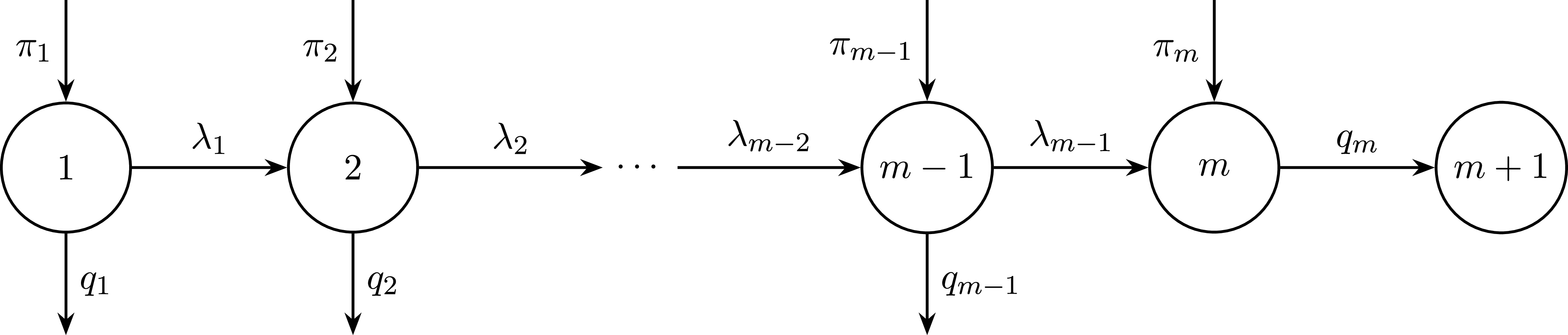
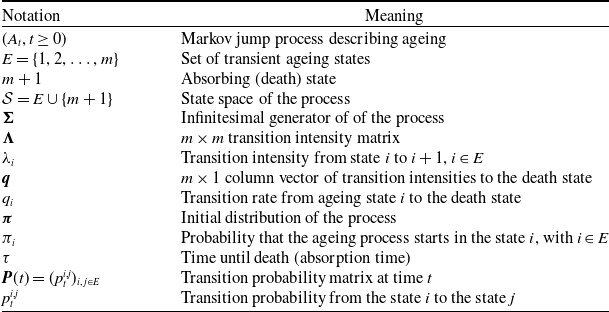
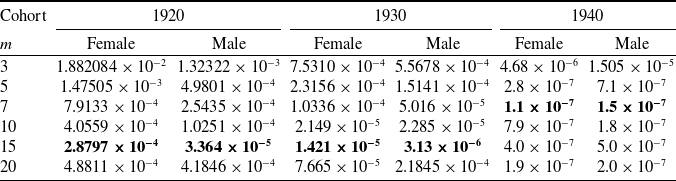
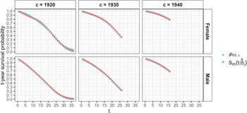
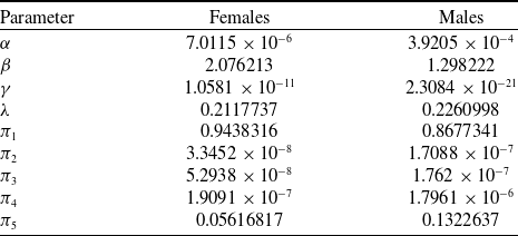




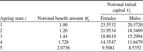


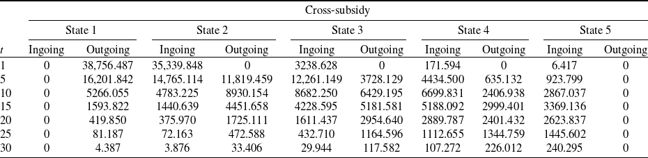


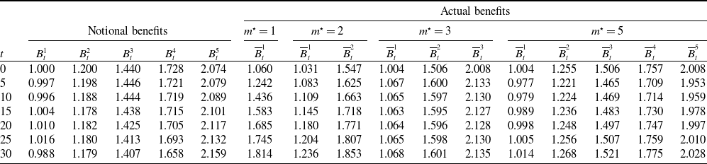


 Open access

