


1. Introduction
Over the past two decades the use of radiocarbon date frequencies to infer population history, referred to as the “dates-as-data” approach, has significantly reshaped archaeological studies. Prior to the adoption of this framework, demographic interpretations often rested on a priori assumptions drawn from population growth models such as logistic or Malthusian trajectories (e.g., Binford and Binford Reference Binford and Binford1969; Boserup Reference Boserup1965; Cohen Reference Cohen and Reed1977; Hassan Reference Hassan1981; Redman Reference Redman1978). Without empirical tools to reconstruct population histories, such studies tended to assume, rather than interrogate, demographic change over time. Although the core idea can be traced back to Rick (Reference Rick1987), the development and application of summed probability distributions (SPDs) catalyzed its integration into archaeology, prompting a broader rethinking of population dynamics in archaeology. Conventional demographic models are increasingly being challenged, as studies employing this approach have documented asynchronous fluctuations, abrupt demographic collapses, and regionally divergent, complicated trajectories (Shennan and Edinborough Reference Shennan and Edinborough2007; Shennan et al. Reference Shennan, Downey, Timpson, Edinborough, Colledge, Kerig, Manning and Thomas2013). It has also encouraged a departure from earlier reliance on typological sequences and the assumed durations of pottery phases (Bevan and Crema Reference Bevan and Crema2021). It is noteworthy that its extensive use has been attributed largely to the construction of large-scale radiocarbon databases across various regions, including AustArch (Williams et al. Reference Williams, Ulm, Smith and Reid2014), CARD (Gajewski et al. Reference Gajewski, Munoz, Peros, Viau, Morlan and Betts2011), EUROEVOL (Manning and Timpson Reference Manning and Timpson2014), NERD (Palmisano et al. Reference Palmisano, Bevan, Lawrence and Shennan2022), RADON (Hinz et al. Reference Hinz, Furholt, Müller, Rinne, Raetzel-Fabian, Sjögren and Wotzka2012), SCAR (Gayo et al. Reference Gayo, Latorre and Santoro2015), p3k14c (Bird et al. Reference Bird, Miranda, Vander Linden, Robinson, Bocinsky, Nicholson, Capriles, Finley, Gayo, Gil, d’Alpoim Guedes, Hoggarth, Kay, Loftus, Lombardo, Mackie, Palmisano, Solheim, Kelly and Freeman2022), MesoRad, as well as databases from Korea (Hwang Reference Hwang2021; Kim and Seong Reference Kim and Seong2022; Oh et al. Reference Oh, Conte, Kang, Kim and Hwang2017; Park et al. Reference Park, Wright and Kim2017; Seong and Kim Reference Seong and Kim2022; Wright et al. Reference Wright, Kim, Park, Yang and Kim2020) and Japan (Kudo Reference Kudo2018; Kudo et al. Reference Kudo, Sakamoto, Hakozaki, Stevens and Crema2023).
However, the dates-as-data approach and the application of SPDs have generated a range of conceptual and methodological challenges. Price et al. (Reference Price, Capriles, Hoggarth, Bocinsky, Ebert and Jones2020) categorize these issues into two groups: the “bias problem” and the “summary problem.” The bias problem was particularly emphasized in early critiques (e.g., Brown Reference Brown2015; Michczyńska and Pazdur Reference Michczyńska and Pazdur2004; Surovell et al. Reference Surovell, Finley, Smith, Brantingham and Kelly2009; Williams Reference Williams2012), which questioned the core assumptions of this method – the presumed correspondence between the frequency of dates and demographic trends. While recognizing its potential of the approach in general, they pointed out that the frequency of radiocarbon dates is critically affected by human behaviors of the past, taphonomic processes, differential preservation, recovery biases, and uneven sampling strategies.
More recent discussions tend to shift toward “summary problems” (e.g., Bamforth and Grund Reference Bamforth and Grund2012; Bronk Ramsey Reference Bronk Ramsey2017; Brown Reference Brown2015; Carleton Reference Carleton2021; Carleton and Groucutt Reference Carleton and Groucutt2021; Contreras and Meadows Reference Contreras and Meadows2014; Heaton Reference Heaton2022; Heaton et al. Reference Heaton, Al-assam and Bard2025; Kerr and McCormick Reference Kerr and McCormick2014; Timpson et al. Reference Timpson, Colledge, Crema, Edinborough, Kerig, Manning, Thomas and Shennan2014, Reference Timpson, Barberena, Thomas, Méndez and Manning2021). Despite their varied emphases, these studies center on two key issues in general: (1) the conceptual validity of SPDs as representations of population trends—because SPDs, the most widely employed tool to summarize radiocarbon datasets, are only sums of measurement uncertainty of discrete individual radiocarbon dates, they risk conflating statistical noise with empirical signals of genuine demographic change (Carleton Reference Carleton2021; Heaton Reference Heaton2022), and (2) the lack of well-defined inferential models and the inherent difficulty of interpreting SPD curves in a statistically formal way (Crema and Shoda Reference Crema and Shoda2021; Timpson et al. Reference Timpson, Barberena, Thomas, Méndez and Manning2021). In response, numerous studies have sought to improve the inferential foundations of analyzing date frequencies or to develop alternative methods. As Crema (Reference Crema2022) reviewed, these efforts include embedding the approach within null hypothesis testing, parametric model fitting, and other formal statistical procedures (Brown Reference Brown2017; Crema and Shoda Reference Crema and Shoda2021; DiNapoli et al. Reference DiNapoli, Crema, Lipo, Rieth and Hunt2021; Price et al. Reference Price, Capriles, Hoggarth, Bocinsky, Ebert and Jones2020; Timpson et al. Reference Timpson, Barberena, Thomas, Méndez and Manning2021). As radiocarbon datasets continue to grow in scale and computational tools improve, the refinement of these methods represents a welcome development.
Yet, over the last decade, the bias problem has received relatively less attention, compared to the intense efforts devoted to the summary problem. This disparity warrants attention, particularly as contemporary demographic research relies ever more heavily on large-scale radiocarbon databases. Although these databases have greatly facilitated archaeological research on population history, significant questions remain regarding the representativeness of the data they contain; data are usually compiled from independently conducted investigations with varying objectives and methodologies. One of the most persistent challenges is heterogeneity in sampling intensity (e.g., Crema Reference Crema2022), arising from disparities in research scope and interests, field methodologies, preservation conditions, and funding (e.g., Becerra-Valdivia et al. Reference Becerra-Valdivia, Leal-Cervantes, Wood and Higham2020; Davies et al. Reference Davies, Holdaway and Fanning2016; Downey et al. Reference Downey, Bocaege, Kerig, Edinborough and Shennan2014; Gayo et al. Reference Gayo, Latorre and Santoro2015; Kerr and McCormick Reference Kerr and McCormick2014; Rhode et al. Reference Rhode, Brantingham, Perreault and Madsen2014; Shennan et al. Reference Shennan, Downey, Timpson, Edinborough, Colledge, Kerig, Manning and Thomas2013; Surovell and Brantingham Reference Surovell and Brantingham2007; Timpson et al. Reference Timpson, Colledge, Crema, Edinborough, Kerig, Manning, Thomas and Shennan2014). Although binning strategies have been proposed to address some of these issues (e.g., Bevan et al. Reference Bevan, Colledge, Fuller, Fyfe, Shennan and Stevens2017; Codding et al. Reference Codding, Roberts, Eckerle, Brewer, Medina, Vernon and Spangler2024; Crema and Bevan Reference Crema and Bevan2021; Shennan et al. Reference Shennan, Downey, Timpson, Edinborough, Colledge, Kerig, Manning and Thomas2013; Timpson et al. Reference Timpson, Colledge, Crema, Edinborough, Kerig, Manning, Thomas and Shennan2014, Reference Timpson, Barberena, Thomas, Méndez and Manning2021), correcting for sampling biases embedded in legacy datasets remains an arduous task. Recent innovations in statistical modeling and hypothesis testing may offer limited inferential utility unless such biases are systematically accounted for.
This study addresses the issue of sampling heterogeneity across settlements/projects and proposes a method for adjusting inter-settlement variation—rescaling the frequency of radiocarbon dates per settlement using dwelling counts. Through simulations of hypothetical populations under diverse conditions, we generate random samples and apply rescaling via mathematical weighting and bootstrap resampling. We then compare the simulated populations, unadjusted samples, and rescaled datasets to assess how rescaling alters the resulting distributions and whether it offers a closer mathematical alignment with the known simulation inputs. Finally, we apply our method to a radiocarbon dataset from Korea to demonstrate how interpretations of demographic dynamics are significantly affected by whether or not rescaling is applied.
To summarize simulated data and visualize their distributions, this study employs SPDs while fully acknowledging their conceptual and methodological caveats (e.g., Bamforth and Grund Reference Bamforth and Grund2012; Bronk Ramsey Reference Bronk Ramsey2017; Brown Reference Brown2015; Carleton Reference Carleton2021; Carleton and Groucutt Reference Carleton and Groucutt2021; Contreras and Meadows Reference Contreras and Meadows2014; Heaton Reference Heaton2022; Heaton et al. Reference Heaton, Al-assam and Bard2025; Kerr and McCormick Reference Kerr and McCormick2014; Timpson et al. Reference Timpson, Colledge, Crema, Edinborough, Kerig, Manning, Thomas and Shennan2014, Reference Timpson, Barberena, Thomas, Méndez and Manning2021). Earlier studies sometimes treated SPD curves as direct reflections of demographic history and occasionally overinterpreted fluctuations without adequately accounting for uncertainties in the calibration process or biases in the underlying data. Today, few archaeologists approach SPDs in such a simplistic manner. In archaeological practice, SPDs remain among the accessible and widely used tools for visually summarizing radiocarbon datasets to explore long-term population trends. We suggest that the value of SPDs lies not in offering exact reconstructions of prehistoric population dynamics, but in serving as visual and heuristic devices for generating hypotheses and guiding further archaeological inquiry. In this study, we do not use SPDs to draw archaeological conclusions; instead, we use them to compare various sample sets and evaluate divergences between hypothetical populations, random sample sets, and adjusted datasets.
2. Sampling biases and the scale of archaeological research of population
Archaeological studies of demographic dynamics using radiocarbon dates span a wide range of spatial and temporal scales, depending on the research question at hand; from highly localized inquiries to continental-scale reconstructions, and from timeframes of several centuries to tens of millennia. Large-scale studies have addressed long-term population fluctuations and continental processes such as the spread of farming (Aurenche et al. Reference Aurenche, Galet, Régagnon-Caroline and Évin2001; Cortell-Nicolau et al. Reference Cortell-Nicolau, Rivas, Crema, Shennan, García-Puchol, Kolář, Staniuk and Timpson2025; Crema et al. Reference Crema, Stevens and Shoda2022; Downey et al. Reference Downey, Bocaege, Kerig, Edinborough and Shennan2014; Oh et al. Reference Oh, Conte, Kang, Kim and Hwang2017; Shennan Reference Shennan, Bocquet-Appel and Bar-Yosef2008; Shennan et al. Reference Shennan, Downey, Timpson, Edinborough, Colledge, Kerig, Manning and Thomas2013; Timpson et al. Reference Timpson, Colledge, Crema, Edinborough, Kerig, Manning, Thomas and Shennan2014; Vander Linden and Silva Reference Vander Linden and Silva2020) as well as supraregional reorganizations of hunter-gatherer populations (Blockley et al. Reference Blockley, Donahue and Pollard2000; Bocquet-Appel et al. Reference Bocquet-Appel, Demars, Noiret and Dobrowsky2005; Codding et al. Reference Codding, Roberts, Eckerle, Brewer, Medina, Vernon and Spangler2024; Crema et al. Reference Crema, Habu, Kobayashi and Madella2016; Freeman et al. Reference Freeman, Hard, Mauldin and Anderies2021; French Reference French2015; Jørgensen et al. Reference Jørgensen, Pesonen and Tallavaara2022; Kim and Seong Reference Kim and Seong2022; Kuzmin and Keates Reference Kuzmin and Keates2005; Schmidt et al. Reference Schmidt, Gehlen, Winkler, Arrizabalaga, Arts, Bicho, Crombé, Eriksen, Grimm, Kapustka, Langlais, Mevel, Naudinot, Nerudová, Niekus, Peresani, Riede, Sauer, Schön, Sobkowiak-Tabaka, Vandendriessche, Weber, Zander, Zimmermann and Maier2025; Schmidt and Zimmermann Reference Schmidt and Zimmermann2019; Seong and Kim Reference Seong and Kim2022; Tallavaara et al. Reference Tallavaara, Pesonen and Oinonen2010). At finer spatial scales, the dates-as-data approach has also proven useful in analyzing local-scale demographic dynamics, including aggregation and dispersion or the emergence and relocation of centers (Birch Reference Birch2012; Crema Reference Crema2013; Manning et al. Reference Manning, Lorentzen and Hart2021; Park et al. Reference Park, Wright and Kim2017; Popescu et al. Reference Popescu, Covătaru, Opriș, Bălășescu, Carozza, Radu, Haită, Sava, Barton and Lazăr2023; Ritchie et al. Reference Ritchie, Ritchie, Blake, Simons and Lepofsky2024; Ritchison Reference Ritchison2020; Ritchison et al. Reference Ritchison, Doubles and Meyers2025; Wright et al. Reference Wright, Kim, Park, Yang and Kim2020). Although sampling bias is a universal concern across all scales of research, the spatiotemporal scale and explanatory scope of a study inevitably influence how datasets are curated and how sampling biases, especially those related to heterogeneous sampling intensity, are addressed.
Among the most widely adopted strategies to control for sampling heterogeneity is the binning method. Introduced over a decade ago (Shennan et al. Reference Shennan, Downey, Timpson, Edinborough, Colledge, Kerig, Manning and Thomas2013), binning has become a standard technique in demographic reconstructions at multiple scales (e.g., Codding et al. Reference Codding, Roberts, Eckerle, Brewer, Medina, Vernon and Spangler2024; Crema et al. Reference Crema, Habu, Kobayashi and Madella2016; Palmisano et al. Reference Palmisano, Bevan and Shennan2017; Timpson et al. Reference Timpson, Colledge, Crema, Edinborough, Kerig, Manning, Thomas and Shennan2014, Reference Timpson, Barberena, Thomas, Méndez and Manning2021). Although the conceptual underpinnings of this method have been critiqued (e.g., Heaton et al. Reference Heaton, Al-assam and Bard2025), its limitations are widely acknowledged (Bevan and Crema Reference Bevan and Crema2021; Crema Reference Crema2022; Crema and Kobayashi Reference Crema and Kobayashi2020; Timpson et al. Reference Timpson, Colledge, Crema, Edinborough, Kerig, Manning, Thomas and Shennan2014). Binning first groups radiocarbon dates into spatial or temporal bins of fixed width. Within each bin, the probability distributions of individual dates are summed, and the result is normalized by dividing by the number of dates per bin. These normalized bin-level SPDs are then aggregated to construct the final SPD curve (Crema Reference Crema2022; Shennan et al. Reference Shennan, Downey, Timpson, Edinborough, Colledge, Kerig, Manning and Thomas2013). The equal weighting of bins reduces the impact of heavily dated loci or periods, thereby mitigating overrepresentation (Crema Reference Crema2022). While especially suited to large-scale studies, binning has also been applied successfully in smaller-scale contexts (e.g., Crema et al. Reference Crema, Habu, Kobayashi and Madella2016; Crema and Kobayashi Reference Crema and Kobayashi2020; Oh and Conte Reference Oh and Conte2022; Park and Kim Reference Park and Kim2024). However, when the objective is to reconstruct settlement-level dynamics particularly at finer scales where variation in site size and their relationships matters, the utility of binning becomes limited. By design, binning is less sensitive to variation in site size or occupation intensity, as it typically involves aggregating and averaging dates within a spatial or temporal bin, thereby equalizing the contribution of each bin regardless of the number of dates it contains.
In sedentary societies composed of multiple settlements, reconstructing spatiotemporal demographic dynamics requires first estimating the lifespans of individual settlements. Archaeologists have long wrestled with how to reliably estimate key parameters of settlement lifespans, such as the timing of initial occupation, the duration of habitation, and fluctuations in population size, and with how to integrate these parameters into broader models of regional settlement patterns. One of the most widely used proxies for estimating settlement-level population history has been dwelling count (Duff and Wilshusen Reference Duff and Wilshusen2000; Hassan Reference Hassan and Schiffer1978; Hill Reference Hill1970; Kirch and Rallu Reference Kirch and Rallu2007; Kolb Reference Kolb1985; Longacre Reference Longacre1975; Ortman and Coffey Reference Ortman and Coffey2017; Parton and Clark Reference Parton and Clark2022; Plog Reference Plog1975; Schacht Reference Schacht1984). Before radiocarbon dating became standard practice, changes in dwelling count were often correlated with ceramic typologies. However, as discussed above and as others have shown (Bevan and Crema Reference Bevan and Crema2021; Crema and Kobayashi Reference Crema and Kobayashi2020; Kolář et al. Reference Kolář, Macek, Tkáč and Szabó2016; Petrie and Lynam Reference Petrie and Lynam2020; Plog and Hantman Reference Plog and Hantman1990), such approaches imposed discrete population models and introduced interpretive uncertainties due to inconsistencies in ceramic phase durations. While some studies attempted to overcome these problems by assuming uniform or normal distributions of dwellings over time (Ortman Reference Ortman2016; Plog Reference Plog1974, Reference Plog1975; Porčić and Nikolić Reference Porčić and Nikolić2016; Roberts et al. Reference Roberts, Mills, Clark, Haas, Huntley and Trowbridge2012; Schacht Reference Schacht1980, Reference Schacht1984), continuous settlement histories remain difficult to reconstruct using pottery chronologies alone.
With the growing availability of radiocarbon data, we propose that the frequency distribution of dated dwellings within a settlement provides an empirically grounded proxy for inferring the settlement’s lifespan. When all (or a sufficiently representative sample of) dwellings are dated, the temporal distribution of those dates can plausibly reflect the duration and demographic trajectory of the settlement’s occupation. If SPDs are employed to summarize these distributions despite their known limitations (Heaton et al. Reference Heaton, Al-assam and Bard2025; Timpson et al. Reference Timpson, Barberena, Thomas, Méndez and Manning2021), then settlement-level SPDs may serve as a more informative proxy than conventional estimates based solely on ceramic phase durations. Within this framework, an overall SPD for a study area can be constructed as the normalized sum of individual settlement-level SPDs. Although cultural and behavioral variables—such as variation in dwelling longevity, the presence of multi-household structures, and degrees of residential mobility—introduce interpretive uncertainty, settlement-level SPDs can be an effective approximation for reconstructing local demographic histories and, in aggregate, broader spatiotemporal population patterns.
Nevertheless, as noted, the number of dated dwellings varies considerably across settlements, countries, and research projects. Without proper adjustment, such variation can distort interpretations by leading to over-or underestimation of settlement size or duration. To address this challenge, we propose a method for correcting inter-settlement variation in sampling intensity. Our approach leverages dwelling count data to rescale radiocarbon datasets, allowing for more proportionate representations of relative population sizes and occupational durations across settlements and presenting new insights into past population structure.
3. Methods
To control for heterogeneity in sampling intensity across settlements, we developed a rescaling approach applied at the settlement level. Our framework implements two closely related procedures: settlement-level weighting and bootstrap resampling. The underlying premise is that each settlement possesses a unique occupation span and demographic history, which can be probabilistically approximated if all dwellings are dated. When only a subset of dwellings is dated, rescaling the temporal distribution of those dates can offer a representative estimate of the full settlement lifespan. Applied systematically across all settlements within a study area, this approach mitigates distortions introduced by uneven sampling intensity.
To evaluate the performance of this rescaling framework in reducing bias, we conducted a series of simulations. Hypothetical populations were generated and subjected to random sampling. The random samples were then rescaled using weighting and bootstrap procedures proportional to settlement size. We compared the resulting SPDs of the sampled and rescaled datasets to those of the hypothetical populations, evaluating the extent to which rescaling improves representativeness.
3.1. Generating hypothetical populations and sampling
We begin by generating populations composed of $K$
dwellings, each of which has a radiocarbon date, distributed across
$K$
dwellings, each of which has a radiocarbon date, distributed across $M$
sedentary settlements. Each settlement,
$M$
sedentary settlements. Each settlement, ${S_i}\left( {i = 1, \ldots, M} \right)$
, contains
${S_i}\left( {i = 1, \ldots, M} \right)$
, contains ${k_i}\left( { \ge5} \right)$
dwellings,
${k_i}\left( { \ge5} \right)$
dwellings, $D_i^{\,j}\left( {j = 1, \ldots, {k_i}} \right)$
, thus
$D_i^{\,j}\left( {j = 1, \ldots, {k_i}} \right)$
, thus $\mathop \sum \nolimits_{i = 1}^M {k_i} = K$
. In this simulation,
$\mathop \sum \nolimits_{i = 1}^M {k_i} = K$
. In this simulation, $K = 1000$
and
$K = 1000$
and $M = 10$
, such that each hypothetical population consists of 1,000 dwellings distributed across 10 settlements (Settlement 1, Settlement 2, … and Settlement 10), with each settlement containing at least five dwellings.
$M = 10$
, such that each hypothetical population consists of 1,000 dwellings distributed across 10 settlements (Settlement 1, Settlement 2, … and Settlement 10), with each settlement containing at least five dwellings.
The simulated datasets—hereafter referred to as “hypothetical populations”—are generated under a range of conditions involving variations in settlement size and lifespan. To introduce variability, settlement sizes ( ${k_i}$
) were drawn from either normal or power-law distributions of dwelling count per settlement, commonly found in empirical data (Duffy Reference Duffy2015; Fletcher Reference Fletcher1986; Johnson Reference Johnson1980). Settlement lifespans were modeled using three distributions—uniform, normal, and skewed (beta distribution,
${k_i}$
) were drawn from either normal or power-law distributions of dwelling count per settlement, commonly found in empirical data (Duffy Reference Duffy2015; Fletcher Reference Fletcher1986; Johnson Reference Johnson1980). Settlement lifespans were modeled using three distributions—uniform, normal, and skewed (beta distribution, $\alpha \; = 2$
,
$\alpha \; = 2$
, $\beta \; = \;5$
). Each dwelling was assigned an uncalibrated radiocarbon date with a standard deviation of 40 years, in accordance with the given conditions.
$\beta \; = \;5$
). Each dwelling was assigned an uncalibrated radiocarbon date with a standard deviation of 40 years, in accordance with the given conditions.
We generate hypothetical populations for two timespans: 600 years (2200–1600 BP) and 1500 years (4500–3000 BP). These different intervals were selected to assess the effects of temporal density of dates (see below), and to avoid the calibration uncertainty associated with the “Hallstatt Plateau” (Pearson et al. Reference Pearson, Pilcher and Baillie1983; Stäuble and Hiller Reference Stäuble and Hiller1997; Wijma et al. Reference Wijma, Aerts, van der Plicht and Zondervan1996), which ranges between circa 2800 and 2400 cal BP. Within each interval, settlement occupation spans (the begin-and end-dates) were randomly assigned: 50–300 years for the 600-year cases and 100–500 years for the 1500-year cases. This yielded 12 hypothetical population models used as null references for comparison (Figures 1 and 2 in Supplementary 1).
Boxplots showing RMSE distances from the hypothetical populations, ${\rm{L}}\left( {\rm{t}} \right)$
, to random sample sets,
${\rm{L}}\left( {\rm{t}} \right)$
, to random sample sets, ${\rm{P}}\left( {\rm{t}} \right)$
: (a) 600 years and (b) 1500 years.
${\rm{P}}\left( {\rm{t}} \right)$
: (a) 600 years and (b) 1500 years.

Figure 1 Long description
Panel A: Boxplots showing RMSE distances from the hypothetical populations to random sample sets over 600 years. The x-axis represents maximum sample fractions in percent (20, 30, 40) and the y-axis represents RMSE. The plots are divided into three columns based on the type of hypothetical population: normal, skewed, and uniform. Each row represents a different type of random sample set: normal and power law. Panel B: Boxplots showing RMSE distances from the hypothetical populations to random sample sets over 1500 years. The x-axis represents maximum sample fractions in percent (20, 30, 40) and the y-axis represents RMSE. The plots are divided into three columns based on the type of hypothetical population: normal, skewed, and uniform. Each row represents a different type of random sample set: normal and power law.
Examples of SPD Comparisons: 600 years, Maximum Sample Fraction 30%, 25-year rolling mean applied.

We note that the probability distribution of calibrated radiocarbon date of dwelling $d_i^{\,j}\left( t \right)$
for each dwelling
$d_i^{\,j}\left( t \right)$
for each dwelling $D_i^{\,j}$
. Then, aggregated probability distribution of dates of each settlement can be defined as
$D_i^{\,j}$
. Then, aggregated probability distribution of dates of each settlement can be defined as
 $${L_i}\left( t \right) = {1 \over K}\sum \limits_{j = 1}^{{k_i}} d_i^{\,j}\left( t \right)\;,$$
and the normalized SPD of the population as
 $$L\left( t \right) = {1 \over K}\mathop \sum \limits_{i = 1}^M \mathop \sum \limits_{j = 1}^{{k_i}} d_i^{\,j}\left( t \right) = \mathop \sum \limits_{i = 1}^M {L_i}\left( t \right).$$
From each hypothetical population, we randomly sampled dwellings from each settlement. Each settlement had a minimum of five samples, and the maximum sampling fraction was set to 20%, 30%, or 40%. Sampling intensity per settlement was randomly determined within these bounds, simulating heterogeneous sampling intensity. Each combination of population model and sampling fraction was replicated 50 times.
Let $P\left( t \right)$
be the normalized SPD from the sampled dataset, where
$P\left( t \right)$
be the normalized SPD from the sampled dataset, where ${n_i}$
is the sample size for settlement
${n_i}$
is the sample size for settlement $i$
and
$i$
and $N = \mathop \sum \nolimits_{i = 1}^M {n_i}$
is the total number of sampled dwellings. The overall SPD and settlement-level SPDs from the sampled data are:
$N = \mathop \sum \nolimits_{i = 1}^M {n_i}$
is the total number of sampled dwellings. The overall SPD and settlement-level SPDs from the sampled data are:
 $$P\left( t \right) = {1 \over N}\mathop \sum \limits_{i = 1}^M \left[ {\mathop \sum \limits_{j = 1}^{{n_i}} d_i^{\,j}\left( t \right)} \right] = \mathop \sum \limits_{i = 1}^M {P_i}\left( t \right),$$
and
 $${P_i}\left( t \right) = {1 \over N}\mathop \sum \limits_{j = 1}^{{n_i}} d_i^{\,j}\left( t \right)$$
, respectively.
3.2. Rescaling: Weighting and bootstrap resampling
To address the issue of uneven sampling intensity across settlements, we propose two rescaling approaches, settlement-level weighting and bootstrap resampling, designed to adjust for disparities between the number of dated dwellings and the total dwelling counts. Both methods aim to approximate the population history that would be inferred if all dwellings within each settlement were dated, thereby mitigating distortions arising from heterogeneous sampling intensities. In the sections that follow, we outline the implementation of each method and describe how they are applied to construct adjusted SPDs.
3.2.1. Weighting
Suppose we have ${n_i}$
sampled dates from
${n_i}$
sampled dates from ${k_i}$
dwellings for each settlement
${k_i}$
dwellings for each settlement ${S_i}$
. The probability density function
${S_i}$
. The probability density function $d_i^{\,j}\left( t \right)$
for each sampled date can be aggregated and weighted at a settlement-level by defining
$d_i^{\,j}\left( t \right)$
for each sampled date can be aggregated and weighted at a settlement-level by defining ${W_i}\left( t \right)$
as
${W_i}\left( t \right)$
as
 $${W_i}\left( t \right) = {{{k_i}} \over K}\left[ {{1 \over {{n_i}}}\mathop \sum \limits_{j = 1}^{{n_i}} d_i^{\,j}\left( t \right)} \right] = \;{{{k_i}N} \over {{n_i}K}}{P_i}\left( t \right)$$
since
 $${P_i}\left( t \right) = {1 \over N}\mathop \sum \limits_{j = 1}^{{n_i}} d_i^{\,j}\left( t \right) = {{{n_i}} \over N}\left[ {{1 \over {{n_i}}}\mathop \sum \limits_{j = 1}^{{n_i}} d_i^{\,j}\left( t \right)} \right]$$
Then, the weighted overall SPD $W\left( t \right)\;$
is
$W\left( t \right)\;$
is $\mathop \sum \nolimits_{i = 1}^M {W_i}\left( t \right)$
.
$\mathop \sum \nolimits_{i = 1}^M {W_i}\left( t \right)$
.
3.2.2. Bootstrap resampling
The second rescaling approach applies the bootstrap method originally proposed by Efron (Reference Efron1979). Bootstrapping is a non-parametric resampling technique that draws samples with replacement from an observed dataset to estimate statistical parameters such as means, variances, and confidence intervals (Aczel Reference Aczel1995). This technique is particularly well suited to small samples with unknown or complex distributions and has been widely applied in archaeological research, including examination of prehistoric population histories (e.g., Downey et al. Reference Downey, Bocaege, Kerig, Edinborough and Shennan2014; Drennan et al. Reference Drennan, Berrey and Peterson2015; Eren et al. Reference Eren, Chao, Hwang and Colwell2012; McLaughlin Reference McLaughlin2019; Price et al. Reference Price, Wolfhagen and Otárola-Castillo2016; Rick Reference Rick1987; Robinson et al. Reference Robinson, Zahid, Codding, Haas and Kelly2019; but see Heaton et al. Reference Heaton, Al-assam and Bard2025 for a critique).
In our study, we employ a modified version of the bootstrap method. For each settlement, we perform resampling with replacement, drawing the number of dates equal to the total count of dwellings in that settlement, repeating this process $b$
times per settlement. With
$b$
times per settlement. With ${k_i}$
dwellings, we get the settlement-level aggregation of resampled data,
${k_i}$
dwellings, we get the settlement-level aggregation of resampled data, ${R_i}\left( t \right)$
,
${R_i}\left( t \right)$
,
 $${R_i}\left( t \right) = {{{k_i}} \over K}\left[ {{1 \over {b{k_i}}}\mathop \sum \limits_{j = 1}^{b{k_i}} d_{i}^{\,j}\left( t \right)} \right]$$
and overall SPD of resampled dataset $R\left( t \right)$
is
$R\left( t \right)$
is $\mathop \sum \nolimits_{i = 1}^M {R_i}\left( t \right)$
.
$\mathop \sum \nolimits_{i = 1}^M {R_i}\left( t \right)$
.
Bootstrap resampling is repeated 30 times per settlement (i.e., $b = 30$
). Unlike standard applications of bootstrapping aimed at estimating population parameters such as mean, standard deviation and confidence interval, our goal is to enhance sample representativeness for SPD generation. Therefore, we pooled the 30 resampled iterations and aggregated them to produce a rescaled probability density function proportional to the total dwelling count of each settlement. This results in a resampled dataset for each settlement that is 30 times larger than the original number of dwellings. The settlement-level probability density functions were then summed to construct an area-wide aggregated SPD reflecting overall demographic trends. For a hypothetical population of 1,000 dwellings across 10 settlements, the procedure generates 30,000 resampled dates per simulation. Then, the results are normalized.
$b = 30$
). Unlike standard applications of bootstrapping aimed at estimating population parameters such as mean, standard deviation and confidence interval, our goal is to enhance sample representativeness for SPD generation. Therefore, we pooled the 30 resampled iterations and aggregated them to produce a rescaled probability density function proportional to the total dwelling count of each settlement. This results in a resampled dataset for each settlement that is 30 times larger than the original number of dwellings. The settlement-level probability density functions were then summed to construct an area-wide aggregated SPD reflecting overall demographic trends. For a hypothetical population of 1,000 dwellings across 10 settlements, the procedure generates 30,000 resampled dates per simulation. Then, the results are normalized.
3.3. Comparison and evaluation
We assess the degree to which the SPDs of sampled and rescaled datasets approximate the hypothetical populations. Specifically, we examine how rescaling affects correspondence with both the overall population-level SPDs, $L\left( t \right)$
, and the individual settlement lifespans,
$L\left( t \right)$
, and the individual settlement lifespans, ${L_i}\left( t \right)$
, relative to random sample sets. We use root mean squared error (RMSE) for a quantitative measure of dissimilarity. It can be evaluated by the square root of the sum of squared differences between the corresponding function values across all time bins as
${L_i}\left( t \right)$
, relative to random sample sets. We use root mean squared error (RMSE) for a quantitative measure of dissimilarity. It can be evaluated by the square root of the sum of squared differences between the corresponding function values across all time bins as
 $$\left\| {f - g} \right\| = \sqrt {{1 \over n}\mathop \sum \limits_{i = 1}^n {{\left|\, {f\left( {{t_i}} \right) - g\left( {{t_i}} \right)} \right|}^2}} $$
where $n$
is the number of time bins, which is 1 year in this study.
$n$
is the number of time bins, which is 1 year in this study.
This metric provides a single scalar value reflecting the overall difference between two distributions. A lower RMSE score indicates a closer match to the reference population. It is particularly useful in our context because it is sensitive to both systematic bias (e.g., temporal shifts in peaks and dips) and stochastic noise (e.g., sampling variation), capturing overall fidelity of the sampled SPD to the target population curve (Scott Reference Scott2015). In each simulation, we calculate RMSE distances from the hypothetical population distributions ( $L\left( t \right)$
and
$L\left( t \right)$
and ${L_i}\left( t \right)$
) to the randomly sampled datasets (
${L_i}\left( t \right)$
) to the randomly sampled datasets ( $P\left( t \right)$
and
$P\left( t \right)$
and ${P_i}\left( t \right)$
), and the rescaled datasets (
${P_i}\left( t \right)$
), and the rescaled datasets ( $W\left( t \right)$
,
$W\left( t \right)$
, ${W_i}\left( t \right)$
,
${W_i}\left( t \right)$
, $R\left( t \right)$
, and
$R\left( t \right)$
, and ${R_i}\left( t \right)$
), respectively. This allows us to evaluate whether rescaling reduces deviation from the true population more effectively than unadjusted random sampling under a variety of conditions. To ensure comparability, all SPDs are normalized prior to RMSE calculation.
${R_i}\left( t \right)$
), respectively. This allows us to evaluate whether rescaling reduces deviation from the true population more effectively than unadjusted random sampling under a variety of conditions. To ensure comparability, all SPDs are normalized prior to RMSE calculation.
4. Results
4.1. Overall change in population size inferred from SPDs
Normalized SPDs derived from random sample sets, $P\left( t \right)$
, exhibit notable variation in shape across the 50 iterations and frequently deviate from the patterns observed in the hypothetical populations (
$P\left( t \right)$
, exhibit notable variation in shape across the 50 iterations and frequently deviate from the patterns observed in the hypothetical populations ( $L\left( t \right)$
), irrespective of the underlying parameters (Figures 3 and 4 in Supplementary 1). Increasing the maximum sampling fraction per settlement enlarges the overall sample size; on average, 122 dates (
$L\left( t \right)$
), irrespective of the underlying parameters (Figures 3 and 4 in Supplementary 1). Increasing the maximum sampling fraction per settlement enlarges the overall sample size; on average, 122 dates ( $s = 19$
) for the 20% cap, 175 (
$s = 19$
) for the 20% cap, 175 ( $s = 33$
) for 30%, and 218 (
$s = 33$
) for 30%, and 218 ( $s = 44$
) for 40%. But, as indicated in Figure 1, it does not consistently reduce variance or improve representativeness. Rather, higher maximum sampling fractions tend to amplify inter-settlement heterogeneity, suggesting that larger sample sizes alone do not necessarily yield closer approximations when sampling intensity is uneven across settlements.
$s = 44$
) for 40%. But, as indicated in Figure 1, it does not consistently reduce variance or improve representativeness. Rather, higher maximum sampling fractions tend to amplify inter-settlement heterogeneity, suggesting that larger sample sizes alone do not necessarily yield closer approximations when sampling intensity is uneven across settlements.
Examples of SPD Comparisons: 1500 years, Maximum Sample Fraction 30%, 50-year rolling mean applied.

Figure 3 Long description
The image contains four line graphs comparing probability density distributions of different sample types over a time span from 5500 to 3100 Cal BP. Each graph represents a different combination of sample types and seeds. Panel A: This line graph shows the probability density distribution for a power law - uniform combination with Seed: 45. The x-axis represents Cal BP (Calibrated Before Present) ranging from 5500 to 3100, and the y-axis represents Probability Density ranging from 0.0000 to 0.0020. The graph includes four lines: Hypothetical Population (gray), Random Sample (blue), Weighted (orange), and Bootstrapped (pink). Panel B: This line graph shows the probability density distribution for a power law - normal combination with Seed: 50. The x-axis represents Cal BP ranging from 5500 to 3100, and the y-axis represents Probability Density ranging from 0.0000 to 0.0030. The graph includes four lines: Hypothetical Population (gray), Random Sample (blue), Weighted (orange), and Bootstrapped (pink). Panel C: This line graph shows the probability density distribution for a power law - skewed combination with Seed: 4. The x-axis represents Cal BP ranging from 5500 to 3100, and the y-axis represents Probability Density ranging from 0.0000 to 0.0020. The graph includes four lines: Hypothetical Population (gray), Random Sample (blue), Weighted (orange), and Bootstrapped (pink). Panel D: This line graph shows the probability density distribution for a normal - uniform combination with Seed: 30. The x-axis represents Cal BP ranging from 5500 to 3100, and the y-axis represents Probability Density ranging from 0.0000 to 0.0030. The graph includes four lines: Hypothetical Population (gray), Random Sample (blue), Weighted (orange), and Bootstrapped (pink).
Comparisons of RMSE distances from the hypothetical populations, ${\rm{L}}\left( {\rm{t}} \right)$
, to random sample sets,
${\rm{L}}\left( {\rm{t}} \right)$
, to random sample sets, ${\rm{P}}\left( {\rm{t}} \right)$
, weighted sample sets,
${\rm{P}}\left( {\rm{t}} \right)$
, weighted sample sets, ${\rm{W}}\left( {\rm{t}} \right)$
, and bootstrap resampled datasets,
${\rm{W}}\left( {\rm{t}} \right)$
, and bootstrap resampled datasets, ${\rm{R}}\left( {\rm{t}} \right)$
.
${\rm{R}}\left( {\rm{t}} \right)$
.

Rescaling the random sample sets in proportion to the number of dwellings per settlement—whether via weighting ( $W\left( t \right)$
) or bootstrap resampling (
$W\left( t \right)$
) or bootstrap resampling ( $R\left( t \right)$
), which yield nearly identical results—consistently produces SPDs that better approximate the original hypothetical populations,
$R\left( t \right)$
), which yield nearly identical results—consistently produces SPDs that better approximate the original hypothetical populations, $L\left( t \right)$
. Figures 2 and 3 show eight representative cases—four from each of the datasets constructed with 600-and 1500-year intervals—selected to illustrate the effect of rescaling. For instance, as shown in Figure 2a, the SPD derived from the random sample set suggests overall population growth with a minor dip around 1900 cal BP. In contrast, both the hypothetical population and the rescaled dataset indicate a marked population decline following 2000 cal BP and a steady recovery from 1850 cal BP. Similarly, in Figure 2c, the rescaled and hypothetical SPDs exhibit a consistent growth trend punctuated by a dip near 1900 cal BP, while the random sample departs noticeably from this trajectory. Figure 3a likewise demonstrates that, whereas the sampled data show a declining trend after 3800 cal BP, the rescaled data better capture the shape of the hypothetical SPD, including another peak around 3400 cal BP.
$L\left( t \right)$
. Figures 2 and 3 show eight representative cases—four from each of the datasets constructed with 600-and 1500-year intervals—selected to illustrate the effect of rescaling. For instance, as shown in Figure 2a, the SPD derived from the random sample set suggests overall population growth with a minor dip around 1900 cal BP. In contrast, both the hypothetical population and the rescaled dataset indicate a marked population decline following 2000 cal BP and a steady recovery from 1850 cal BP. Similarly, in Figure 2c, the rescaled and hypothetical SPDs exhibit a consistent growth trend punctuated by a dip near 1900 cal BP, while the random sample departs noticeably from this trajectory. Figure 3a likewise demonstrates that, whereas the sampled data show a declining trend after 3800 cal BP, the rescaled data better capture the shape of the hypothetical SPD, including another peak around 3400 cal BP.
Figure 4 presents boxplots of RMSE scores across all experimental conditions. In nearly all cases, rescaled datasets show lower RMSE values and smaller variances, indicating not only improved fidelity to the target population but also reduced susceptibility to sampling noise. Table 1 summarizes the comparative performance of the rescaling approaches. Across 1,800 iterations, the rescaled datasets yielded lower RMSE scores in 1,704 cases (94.7%) for weighting and in 1,702 cases (94.6%) for resampling. Both two-sample t-tests and pairwise Wilcoxon signed-rank tests confirm the statistical significance of these differences (t-test, $p \lt 0.0001$
; Wilcoxon signed-rank test,
$p \lt 0.0001$
; Wilcoxon signed-rank test, $p \lt 0.0001$
). A closer look at Table 1 reveals that the efficacy of rescaling improves incrementally with higher maximum sampling fractions and longer temporal durations. In the 600-year simulations, rescaled datasets yield lower RMSE scores than random samples in 265 to 286 of 300 iterations for weighting and in 262 to 286 of 300 iterations for resampling. This becomes more pronounced in the 1500-year simulations, where the number of successful cases rises to between 292 and 295 for weighting and between 292 and 296 for resampling. For both durations, higher sampling fraction, which in general implies greater inter-settlement heterogeneity in sampling intensity, tends to result in rescaling more consistently reducing RMSE.
$p \lt 0.0001$
). A closer look at Table 1 reveals that the efficacy of rescaling improves incrementally with higher maximum sampling fractions and longer temporal durations. In the 600-year simulations, rescaled datasets yield lower RMSE scores than random samples in 265 to 286 of 300 iterations for weighting and in 262 to 286 of 300 iterations for resampling. This becomes more pronounced in the 1500-year simulations, where the number of successful cases rises to between 292 and 295 for weighting and between 292 and 296 for resampling. For both durations, higher sampling fraction, which in general implies greater inter-settlement heterogeneity in sampling intensity, tends to result in rescaling more consistently reducing RMSE.

4.2. Lifespans of individual settlements and inter-settlement relationships
The issue of heterogeneous sampling intensity presents a more serious challenge when interpreting the organization of settlements using radiocarbon datasets. Spatial analyses that aim to investigate demographic dynamics—such as inter-settlement relationships, aggregation and dispersion processes, and the emergence or relocation of central places—rely on reliable estimation of individual settlement size and duration.
Figure 5 presents selected cases from our simulation, illustrating aggregated probability distributions for ten individual settlements. In these cases, the probability distributions derived from random samples ( ${P_i}\left( t \right)$
) over-or underrepresent the size and occupation span of settlements. Figures 5 and 6 together reveal how such distortions in the temporal representation of individual settlements can mislead interpretations of both spatial dynamics and broader population trends. By contrast, rescaling the random samples in proportion to the number of dwellings per settlement,
${P_i}\left( t \right)$
) over-or underrepresent the size and occupation span of settlements. Figures 5 and 6 together reveal how such distortions in the temporal representation of individual settlements can mislead interpretations of both spatial dynamics and broader population trends. By contrast, rescaling the random samples in proportion to the number of dwellings per settlement, ${W_i}\left( t \right)$
and
${W_i}\left( t \right)$
and ${R_i}\left( t \right)$
, yields probability distributions that more closely approximate the actual temporal profiles of the simulated settlements,
${R_i}\left( t \right)$
, yields probability distributions that more closely approximate the actual temporal profiles of the simulated settlements, ${L_i}\left( t \right)$
.
${L_i}\left( t \right)$
.
Examples of Settlement SPDs: (a) Power-law & Normal distribution, (b) Power-law & Skewed distribution (600 years, Maximum Sample Fraction 30%, 25-year rolling mean applied). For details of settlements, see Table 2 in Supplementary 1.

Figure 5 Long description
Panel A: This panel contains four density plots comparing settlement SPDs for a power-law and normal distribution. The plots are labeled as Hypothetical Population, Random Sample, Weighted, and Bootstrapped. Each plot shows probability density on the vertical axis and Cal BP (calibrated years before present) on the horizontal axis. Different colored areas represent different settlements, with a legend indicating settlements 1 through 10. The Hypothetical Population plot shows multiple peaks, particularly around 2000 and 1500 Cal BP. The Random Sample plot also shows peaks around these times but with different distributions. The Weighted and Bootstrapped plots show similar patterns to the Hypothetical Population but with variations in peak heights and positions. Panel B: This panel contains four density plots comparing settlement SPDs for a power-law and skewed distribution. The plots are labeled similarly: Hypothetical Population, Random Sample, Weighted, and Bootstrapped. The axes and legend are the same as in Panel A. The Hypothetical Population plot shows prominent peaks around 2000 and 1500 Cal BP. The Random Sample plot shows similar peaks but with different distributions. The Weighted and Bootstrapped plots show variations in peak heights and positions, similar to the patterns observed in Panel A.

In Figure 5a (600-year timespan), the random sample set underrepresents Settlement 1 spanning roughly from 2200 to 1800 cal BP, and overrepresents Settlement 2 (see Figures 1 and 2 in Supplementary 1, for detailed information about simulated settlements). Figure 5b illustrates the considerable underrepresentation of Settlement 1, along with overrepresentation of Settlements 2 and 4 when an SPD is produced using the random sample set. A comparable pattern is observed in the 1500-year timespan. In Figure 6a, Settlement 1 (ca. 3500–3000 cal BP) is significantly underrepresented in the random sample, while Settlement 4 is overrepresented. In Figure 6b, Settlement 1 (spanning ca. 5000–4500 cal BP), the largest among the ten, is again underrepresented. In all cases, the rescaled datasets more faithfully reconstruct the original lifespans and relative size of the settlements. Figure 7 confirms this trend. Random sample sets consistently yield higher RMSE scores and greater variance compared to rescaled datasets across all settlements. Severe misrepresentation is most likely when small sample sizes are drawn from large settlements, or vice versa, particularly in power-law distribution of settlement size. Settlement 1 ( $n = 363$
) and Settlement 2 (
$n = 363$
) and Settlement 2 ( $n = 183$
), the largest settlements (Table 1 in Supplementary 1), show higher mean RMSE scores and greater variances, indicating heightened susceptibility to sampling bias. In contrast, rescaling consistently lowers both the average RMSE distances and their variability across all settlements.
$n = 183$
), the largest settlements (Table 1 in Supplementary 1), show higher mean RMSE scores and greater variances, indicating heightened susceptibility to sampling bias. In contrast, rescaling consistently lowers both the average RMSE distances and their variability across all settlements.
Comparisons of RMSE distances from the hypothetical populations, ${{\rm{L}}_{\rm{i}}}\left( {\rm{t}} \right)$
, to random sample sets,
${{\rm{L}}_{\rm{i}}}\left( {\rm{t}} \right)$
, to random sample sets, ${{\rm{P}}_{\rm{i}}}\left( {\rm{t}} \right)$
, weighted sample sets,
${{\rm{P}}_{\rm{i}}}\left( {\rm{t}} \right)$
, weighted sample sets, ${{\rm{W}}_{\rm{i}}}\left( {\rm{t}} \right)$
and bootstrapped datasets,
${{\rm{W}}_{\rm{i}}}\left( {\rm{t}} \right)$
and bootstrapped datasets, ${{\rm{R}}_{\rm{i}}}\left( {\rm{t}} \right)$
by settlement: (a) 600 years (b) 1500 years (Maximum Sample Fraction 30%)
${{\rm{R}}_{\rm{i}}}\left( {\rm{t}} \right)$
by settlement: (a) 600 years (b) 1500 years (Maximum Sample Fraction 30%)

5. Case study: Demographic dynamics in the proto- and early historical periods of Korea
Our experiments reveal that rescaling consistently produces SPDs that better approximate those of hypothetical populations, providing different interpretations of population history. We apply our rescaling method to radiocarbon datasets from archaeological sites in Korea dating to the proto- and early historical periods. Beginning in 1C BC, Korea witnessed a significant increase in social complexity, driven primarily by the introduction of iron technology from China, which was applied to agricultural tools and weaponry. This period, termed the Proto–Three Kingdoms period (1C BC–AD 3C), saw rapid population growth and the emergence of numerous competing polities. This shift eventually led to the formation of three ancient states by late AD 3C, inaugurating the Three Kingdoms period (AD 4–7C). According to both Korean and contemporaneous Chinese historical sources, Baekje—one of the three kingdoms—originated as a small polity in present-day Seoul. Historical texts suggest that it developed into a centralized state by expanding southward through military conquest and/or political consolidation (Kim Reference Kim1998 [1145]; Noh Reference Noh1987). This expansion is archaeologically supported by the spread of Baekje-style pottery and tomb types across central-western and southwestern Korea (Kim Reference Kim2007; Kwon Reference Kwon2001; Lee Reference Lee2022; Park Reference Park2001, Reference Park2007). By AD 6C, peripheral areas were increasingly incorporated into Baekje’s domain, though the timing and character of these processes remain subjects of debate (for a recent overview, see Kim Reference Kim2024). The southward advance of Baekje appears to have entailed reorganizations of settlement patterns in the peripheries, including the emergence and relocation of population concentrations (Park et al. Reference Park, Wright and Kim2017; Wright et al. Reference Wright, Kim, Park, Yang and Kim2020).
For this case study, we examine two areas: the upper-middle Yeongsan River Basin in the southwestern and the upper Geum River Basin in central-western Korea (Figure 8). Since the early 2000s, extensive archaeological surveys and excavations, largely prompted by government-led infrastructure development and river refurbishment projects, have uncovered a wide array of settlements in both areas, ranging from small hamlets to large villages with more than 1000 pit dwellings. While most excavations have been undertaken by cultural resource management (CRM) firms, the Bureau of Cultural Heritage of the South Korean government supervises all stages of investigation to ensure methodological consistency and reporting quality. By national regulation, excavation reports must be published and made publicly available within two years of completion. As of 2024, the number of published radiocarbon dates in South Korea stands at approximately 20,000, making it one of the most comprehensive and densely sampled radiocarbon databases globally (Hwang Reference Hwang2021; Kim and Seong Reference Kim and Seong2022; Oh et al. Reference Oh, Conte, Kang, Kim and Hwang2017; Park et al. Reference Park, Wright and Kim2017; Seong and Kim Reference Seong and Kim2022; Wright et al. Reference Wright, Kim, Park, Yang and Kim2020). In the dataset, 3561 dates from dwellings between 2100 and 1500 BP are reported from 481 sites across South Korea, which cover the period of interest in this study.
Study areas and sites: (a) Locations. (b) The Geum River Basin. (1. Bokryong-dong-1; 2. Bokryong-dong-2; 3. Bongmyeong-dong; 4. Daepyong-ri; 5. Juk-dong; 6. Naseong-ri; 7. Songjeol-dong; 8. Yonggye-dong; 9. Yongho-Hapgang-ri) (c) The Yeongsan River Basin. (1. Dongnim-dong; 2. Hanam-dong; 3. Heukseok-dong; 4. Oseon-dong; 5. Sanjeong-dong; 6. Seonam-dong; 7: Sinchang-dong; Taemok-ri; 9: Yeonsan-dong; 10. Yongdu-dong; 11. Yongsan-dong)

Figure 8 Long description
Panel A: A map of Korea highlighting the locations of the Geum River Basin and Yeongsan River Basin. The map includes a small inset showing the location of Korea in East Asia. Seoul is marked, and the surrounding bodies of water, the Yellow Sea and the East Sea, are labeled. Panel B: A detailed map of the Geum River Basin with numbered sites (1 to 9) marked within the basin. The basin boundaries are outlined in red, and elevation is indicated with shading. Panel C: A detailed map of the Yeongsan River Basin with numbered sites (1 to 11) marked within the basin. The basin boundaries are outlined in red, and elevation is indicated with shading.
We selected settlements with at least five dated dwellings from the study areas. Published radiocarbon dates were critically assessed and filtered to retain only those directly associated with dwellings attributable to the Proto- and Early Three Kingdoms periods. Anomalous or archaeologically questionable dates were excluded. In cases where multiple dates were obtained from a single dwelling, the results were statistically combined to avoid overrepresentation. We then applied our rescaling procedures to the filtered datasets for each area and produced SPD and spatiotemporal KDE analyses using the R package rcarbon (Crema and Bevan Reference Crema and Bevan2021). Details about the settlements selected for this study, including locations, number of dwellings, dates, and sample fractions, are provided in Supplementary 2.
5.1. The Yeongsan River Basin
In the Yeongsan River Basin, we analyze 142 filtered radiocarbon dates drawn from eleven settlements comprising a total of 3,287 dwellings. The proportion of dated dwellings varies widely between settlements, ranging from 1.34% to 76.92% (Table 2 in Supplementary 2). The overall SPDs of the original and rescaled datasets (Figure 9a) both depict a general trend of population growth from 2000 to 1750 cal BP, followed by a rapid increase peaking around 1700 cal BP and stabilization thereafter, with a minor dip near 1650 cal BP, which would be negligible.
Analytic result of the Yeongsan River Basin. (a) Overall SPD; (b) Probability Distributions of Settlements (Site numbers correspond to Figure 8); (c) KDE analyses over time.

However, when disaggregated to the level of individual settlements, the two datasets diverge remarkably (Figure 9b). The unrescaled data imply that, prior to 1700 cal BP, populations were relatively evenly distributed across small, similarly sized settlements, until the Yeonsan-dong settlement (No. 9) in the southern basin rapidly emerged as the dominant center. By contrast, the rescaled data indicate that the Taemok-ri (No. 8) in the north was the largest and most populous settlement until around 1700 cal BP, after which Yeonsan-dong and Oseon-dong (No. 4) expanded abruptly, giving rise to a coexistence of tripartite population centers.
These divergent reconstructions of the population history are also evident in the KDE analysis (Figure 9c). The unrescaled original dataset highlights the emergence of a new population concentration in the southern basin, with a southwestward shift beginning around 1800 cal BP. The rescaled dataset, however, suggests that the Taemok-ri settlement remained a major population center well after 1700 cal BP, coexisting with other concentrations in the middle basin.
5.2. The Geum River Basin
In the Geum River Basin, we analyze 195 filtered radiocarbon dates from nine settlements comprising a total of 1,442 dwellings. The overall sampling fraction was 13.6%, higher than that of the Yeongsan River Basin, but with considerable variation across individual settlements, ranging from 1.8% to 42.1% (Table 3 in Supplementary 2). Notably, 119 dates were reported from the Songjeol-dong settlement in the northern part of the basin.
At the aggregate level, the SPDs of the original and rescaled datasets both show general population growth until 1700 cal BP, followed by stabilization (Figure 10a). However, the growth trajectories and relative magnitudes differ between the datasets. The probability distributions of individual settlements diverge dramatically, yielding contrasting population histories (Figure 10b). The unrescaled original dataset portrays Songjeol-dong (No. 7) as a dominant population center from 1800 to 1650 cal BP. In contrast, the rescaled dataset indicates that Yonggye-dong (No. 8), located in the south, was the largest settlement from 1950 to 1800 cal BP, after which it dissolved rapidly as Songjeol-dong rose as the principal settlement. These differences are further underscored by the KDE analysis (Figure 10c). The unrescaled original data suggest that Songjeol-dong sustained the largest population throughout the period, whereas the rescaled data show high population density in the south (Yonggye-dong) prior to 1800 cal BP, followed by a sharp demographic shift toward the north (Songjeol-dong).
Analytic result of the Geum River Basin. (a) Overall SPD; (b) Probability Distributions of Settlements (Site numbers correspond to Figure 8); (c) KDE analyses over time.

Figure 10 Long description
Panel A: A line graph titled 'Total SPD Comparison' displays the normalized summed probability distribution (SPD) over time, with the x-axis labeled 'cal BP' ranging from 2200 to 1400 and the y-axis labeled 'Normalized SPD'. Three lines represent different data treatments: "Unrescaled original" in orange, 'Bootstrapped' in dashed black, and 'Weighted' in dotted black. The graph shows trends in SPD over time, with notable peaks around 1800 cal BP. Panel B: Three probability density graphs titled 'Unrescaled original', 'Bootstrapped', and 'Weighted' show the probability density of different settlements over time. Each graph has the x-axis labeled 'cal BP' ranging from 2200 to 1400 and the y-axis labeled 'Probability Density'. Different colored areas represent various settlements, with labels and corresponding colors listed in the legend. Notable peaks and overlaps in probability densities are visible. Panel C: Two sets of heat maps titled 'Unrescaled original' and 'Bootstrapped' show kernel density estimation (KDE) analyses over different years (2100, 2000, 1900, 1800, 1700, 1600, and 1500). Each heat map displays the density distribution across a geographical area, with color gradients indicating density levels.", "EDH": "
The disparities between the two reconstructions are largely attributed to differential sampling fractions (Supplementary 2). Yonggye-dong, which was occupied earlier, had a low sample fraction (eight dates from 448 dwellings; 1.8%), whereas the sample fraction of Songjeol-dong, the population of which increased substantially only after 1800 cal BP, is much higher (119 dates from 558 dwellings; 21.3%). These imbalances likely contribute to significant underrepresentation of the earlier-occupied Yonggye-dong (Figure 10b).
To summarize, the case studies of the Yeongsan and Geum River Basins demonstrate that the use of unadjusted radiocarbon datasets can lead to significantly different reconstructions of local population histories than those produced through rescaling. Although it is not possible to determine whether the rescaled SPDs better reflect past demographic realities, they provide reconstructions more consistent with the established ceramic chronology of the region (Cho Reference Cho2007; Kim Reference Kim2000, Reference Kim2007; Lee Reference Lee2011; Yun Reference Yun2014) than those generated by SPDs based on random sampling alone.
6. Discussion
Recent methodological developments of the dates-as-data approach (e.g., Carleton Reference Carleton2021; Crema Reference Crema2022; Heaton Reference Heaton2022; Heaton et al. Reference Heaton, Al-assam and Bard2025; Timpson et al. Reference Timpson, Barberena, Thomas, Méndez and Manning2021) have enhanced its statistical rigor. These studies advocate embedding demographic inference within formal modeling frameworks, including null hypothesis testing and model fitting. Moving beyond the direct application of unidirectional population growth models or null-hypothesis testing, more recent research (e.g., Crema and Shoda Reference Crema and Shoda2021; DiNapoli et al. Reference DiNapoli, Crema, Lipo, Rieth and Hunt2021; Price et al. Reference Price, Capriles, Hoggarth, Bocinsky, Ebert and Jones2020; Timpson et al. Reference Timpson, Barberena, Thomas, Méndez and Manning2021) has attempted to model population fluctuations. These represent important methodological advancements; however, several key issues warrant further consideration.
First, current methodological studies predominantly focus on changes in total population size over time at a macro-scale. While understanding such broad-scale trends is essential, we argue that, from an archaeological perspective, this captures only one dimension of past demographic dynamics. Many fundamental research questions in archaeological demography concern population reorganization, including processes such as relocations (Kim and Seong Reference Kim and Seong2022; Seong and Kim Reference Seong and Kim2022), community aggregation and dispersion (Barrier Reference Barrier2017; Birch Reference Birch2012; Feinman and Neitzel Reference Feinman and Neitzel2023; Gyucha Reference Gyucha2019; Haggis Reference Haggis and Birch2013; Kohler et al. Reference Kohler, VanBuskirk and Ruscavage-Barz2004; Whallon Reference Whallon2006), the emergence and decline of regional centers (Hill et al. Reference Hill, Clark, Doelle and Lyons2004; Kohler and Varien Reference Kohler and Varien2012; Ortman et al. Reference Ortman, Cabaniss, Sturm and Bettencourt2015; Ortman and Coffey Reference Ortman and Coffey2017; Park et al. Reference Park, Wright and Kim2017; Smith Reference Smith2023; Wright et al. Reference Wright, Kim, Park, Yang and Kim2020), and shifts in settlement hierarchies or heterarchies (Duffy Reference Duffy2015; Kowalewski Reference Kowalewski and Birch2014; Peterson and Drennan Reference Peterson and Drennan2005). These population dynamics are critical for understanding sociopolitical integration, economic interaction, and land-use strategies; yet they may occur with little or no net change in overall population size.
More importantly, the reliability of population reconstructions is not guaranteed by the application of statistically rigorous summary methods alone. While techniques such as null hypothesis testing and model fitting are valuable for evaluating the structure and potential biases of SPDs, they do not automatically transform biased datasets into explanatory models. A critical issue concerns the representativeness of radiocarbon data and the sampling biases inherent in legacy datasets, which significantly affect interpretive validity. As interest in past population dynamics has grown and the dates-as-data approach has become increasingly widespread, particularly alongside the construction of radiocarbon databases, greater attention must be devoted to addressing these limitations.
Given these challenges, an important question arises: how can known biases, particularly those arising from uneven sampling intensity, be managed? To address this issue, we developed and tested a rescaling method aimed at mitigating sampling heterogeneity at the level of individual settlements. We compared SPDs generated from hypothetical populations, randomly sampled datasets (the archaeologist’s practical analogue), and rescaled datasets. SPDs were used not as direct measures of population change but as heuristic tools to demonstrate how significantly summary results can diverge between actual populations and sampled data, and to evaluate whether rescaling can recover the original demographic signals.
Our simulations indicate that rescaled datasets, adjusted using dwelling counts of individual settlements, consistently yield SPDs that more closely approximate the demographic trajectories of hypothetical populations than do unadjusted random samples. The simulation results proved robust across a variety of conditions, including different settlement size distributions (normal vs. power-law), varied settlement lifespans (uniform, normal, skewed), and differing temporal spans (600 vs. 1500 years). Although rescaling can amplify distortions—as correctly noted by McLaughlin (Reference McLaughlin2019) and Heaton et al. (Reference Heaton, Al-assam and Bard2025) —especially when the original datasets are already highly biased, such instances were rare in our simulations: only 96 cases (5.3%) for weighting and 98 (5.4%) for resampling out of 1,800 total iterations (Table 1). In over 94% of cases, rescaling reduced RMSE scores between sample SPDs and reference populations, confirming its general effectiveness.
The benefits of rescaling become more pronounced as sampling heterogeneity across settlements increases. While increasing the maximum sample fraction per settlement raises total sample size, it does not necessarily improve demographic approximations unless inter-settlement sampling heterogeneity is addressed. Rescaling performs particularly well under conditions of low temporal density. In our 1500-year simulations, it achieved 97–98% improvement, compared to 87–95% in the 600-year simulations—suggesting that rescaling is especially effective when the temporal density of sampled radiocarbon dates is low.
These advantages are especially evident in reconstructing inter-settlement dynamics. As emphasized in prior studies (e.g., Bevan and Crema Reference Bevan and Crema2021; Birch-Chapman and Jenkins Reference Birch-Chapman and Jenkins2019; Brown et al. Reference Brown, Reed and Glowacki2013; Crown Reference Crown1991; Dewar Reference Dewar1991; Drennan et al. Reference Drennan, Berrey and Peterson2015; Petrie and Lynam Reference Petrie and Lynam2020; Plog Reference Plog1974, Reference Plog1975; Prentiss et al. Reference Prentiss, Lenert, Foor, Goodale and Schlegel2003; Schacht Reference Schacht1984; Shott Reference Shott1992; Varien et al. Reference Varien, Ortman, Kohler, Glowacki and Johnson2007), estimating the duration and intensity of occupation at individual settlements constitutes a crucial first step toward understanding regional population organization, including the formation, relocation, and dissolution of population centers. Our simulation suggests that SPDs based on radiocarbon dates from dwellings, particularly when rescaled relative to dwelling counts, can serve as reasonable proxies for reconstructing settlement occupation histories. They further show that even when only five radiocarbon dates are available per settlement, rescaling significantly reduces both RMSE values and variance in SPD-based reconstructions. This effect is especially critical for large settlements: without rescaling, they may be severely underrepresented, leading to misinterpretations of broader demographic organization (e.g., Settlements 1 and 2 in power-law distributions; see Figures 5 and 6). We do not claim that rescaling inherently “improves” the quality of radiocarbon datasets in reconstructing demographic dynamics that are ultimately unknowable. Rather, we suggest that controlling for sampling heterogeneity through rescaling may generate alternative hypotheses and pose new research questions for future archaeological investigation.
Our case study further demonstrates how sampling heterogeneity can skew empirical interpretations of demographic dynamics. The unrescaled original and rescaled datasets yielded markedly different reconstructions of population reorganization during Baekje’s expansion in proto- and early historical Korea. While they do not produce significantly different overall population trajectories for the Yeongsan and Geum River Basins, the spatial and temporal configurations of population concentrations diverge substantially (see above). These discrepancies are largely attributable to low sample fractions in the largest settlements: only 21 of 1043 dwellings in Taemok-ri (2.01%) and 8 of 448 in Yonggye-dong (1.8%) were dated (Table 1 in Supplementary 2), resulting in substantial underestimation of population size of these population concentrations. The apparent stability in population size reflected in the overall SPD for the Yeongsan River Basin (Figure 9a), despite the underrepresentation of Taemok-ri, is likely due to the relatively high sampling fractions in smaller contemporaneous settlements (for instance, Shinchang-dong, where 10 of 13 dwellings were dated) which inadvertently compensated for the deficit. Although definitive validation remains challenging, the patterns from the rescaled dataset align more closely with interpretations based on Korean pottery chronologies (Cho Reference Cho2007; Kim Reference Kim2000, Reference Kim2007; Lee Reference Lee2011; Yun Reference Yun2014). This highlights a critical point: even when overall SPDs appear consistent and robust, uncorrected inter-settlement sampling heterogeneity poses a significant risk of producing fundamentally incongruent archaeological interpretations of spatial reorganization.
Combining radiocarbon dates and dwelling counts to explore population history is not entirely new. Crema and Kobayashi (Reference Crema and Kobayashi2020), for example, analyzed a large dataset of pit dwellings from the central Japanese Jomon, using Bayesian models of ceramic phases. In their framework, dwelling counts served as an independent demographic proxy modeled in parallel with radiocarbon-based inference. Our approach, by contrast, differs in both rationale and implementation. We do not treat dwelling counts as a separate proxy but use them as a corrective factor to address inter-settlement sampling heterogeneity, thereby mitigating biases potentially inherent in given datasets. Where sampling intensity is heterogeneous and variation in settlement size and lifespan is central to the research question, rescaling can be applied to datasets prior to formal modeling. Thus, rescaling and modeling are complementary.
Conceptually, our rescaling method shares objectives with binning strategies, though it differs in emphasis (Crema Reference Crema2022; Shennan et al. Reference Shennan, Downey, Timpson, Edinborough, Colledge, Kerig, Manning and Thomas2013; Timpson et al. Reference Timpson, Colledge, Crema, Edinborough, Kerig, Manning, Thomas and Shennan2014). Binning seeks to equalize contributions of sites regardless of sample size, reducing overrepresentation of intensively dated loci or periods. It primarily addresses variation in site density (Crema Reference Crema2022; Shennan et al. Reference Shennan, Downey, Timpson, Edinborough, Colledge, Kerig, Manning and Thomas2013; Timpson et al. Reference Timpson, Colledge, Crema, Edinborough, Kerig, Manning, Thomas and Shennan2014), proving effective in large-scale studies. In contrast, our method targets relative population size, occupation duration, and historical trajectory at the settlement level. It is particularly suited to finer-scale demographic studies of sedentary societies, where inter-site population dynamics are critical. Despite differences in focus, rescaling and binning can serve distinct yet synergistic roles, with their applicability shaped by the specific research question and analytical scale.
Nonetheless, we acknowledge that rescaling has limitations. Its effectiveness depends on the assumption that dwelling counts are meaningfully related to population size and occupation span—an assumption vulnerable to taphonomic biases, incomplete excavation, multi-household structures, or variability in dwelling use duration. Moreover, the method may be infeasible where dwelling count data are unavailable. Expanding the applicability of rescaling will require alternative proxies, such as settlement area (Downey et al. Reference Downey, Bocaege, Kerig, Edinborough and Shennan2014; Drennan et al. Reference Drennan, Berrey and Peterson2015), total house floor area (Kuijt and Marciniak Reference Kuijt and Marciniak2024; Naroll Reference Naroll1956), artifact quantity or density (Gallivan Reference Gallivan2002; Kohler and Blinman Reference Kohler and Blinman1987; Ortman and Cooper Reference Ortman and Cooper2021), or integrated environmental and archaeological indicators—all of which pose interpretive challenges. While our method addresses inter-settlement or project-level sampling heterogeneity, it does not resolve broader structural biases. Differences in survey coverage, excavation strategy, reporting practices, and research agendas can introduce systematic and often invisible distortions (Crema et al. Reference Crema, Stevens and Shoda2022). Future research may incorporate such biases into rescaling frameworks.
7. Final remarks
The continued construction and use of large radiocarbon databases have created significant opportunities for investigating population dynamics in archaeology. However, because these datasets usually comprise samples submitted independently by numerous researchers with diverse aims, research strategies and focuses, they remain susceptible to various biases including heterogeneous sampling intensity across projects and sites. Despite commendable and ongoing efforts to improve data hygiene (Bevan and Crema Reference Bevan and Crema2021; Bird et al. Reference Bird, Miranda, Vander Linden, Robinson, Bocinsky, Nicholson, Capriles, Finley, Gayo, Gil, d’Alpoim Guedes, Hoggarth, Kay, Loftus, Lombardo, Mackie, Palmisano, Solheim, Kelly and Freeman2022; Fernández-López de Pablo et al. Reference Fernández-López de Pablo, Gutiérrez-Roig, Gómez-Puche, McLaughlin, Silva and Lozano2019; Palmisano et al. Reference Palmisano, Bevan, Lawrence and Shennan2022), it remains a practical challenge when working with aggregated legacy datasets.
In this study, we have proposed a simple, straightforward method for addressing this issue: rescaling radiocarbon data using settlement-level weighting and bootstrap resampling based on dwelling counts. Our approach aligns with multi-proxy frameworks (e.g., French Reference French2015; Lawrence et al. Reference Lawrence, Palmisano and de Gruchy2021; Schmidt et al. Reference Schmidt, Hilpert, Kretschmer, Peters, Broich, Schiesberg, Vogels, Wendt, Zimmermann and Maier2021; Schmidt and Zimmermann Reference Schmidt and Zimmermann2019), which incorporate diverse datasets and methodologies to assess and mitigate interpretive bias. While our method alone does not eliminate all sources of error, we hope it contributes to improving the reliability and resolution of demographic inferences drawn from radiocarbon dates. By integrating rescaling into broader analytical workflows, archaeologists can produce more robust reconstructions of past population dynamics at both local and regional scales.
Supplementary material
To view supplementary material for this article, please visit https://doi.org/10.1017/RDC.2026.10203
Data accessibility
Data and reproducible code for all analyses discussed in the paper can be found at https://github.com/s3jin33/RescalingRadiocarbonData
Acknowledgments
This work was supported by the Research Grant from Seoul National University (100–20230150). We thank Matthew Conte and an anonymous reviewer for valuable comments on earlier versions of this paper.
Author contributions
Jiyoung Park: writing-original draft, analysis, data curation, investigation.
Sejin Kim: writing-original draft, analysis, investigation, visualization.
Taechang Jo: writing-original draft, methodology, validation.
Jangsuk Kim: conceptualization, writing-original draft, methodology, funding acquisition, supervision.
Declarations of interest
The authors have no conflicts of interest to declare.

 L(t)
L(t) P(t)
P(t)


 L(t)
L(t) P(t)
P(t) W(t)
W(t) R(t)
R(t)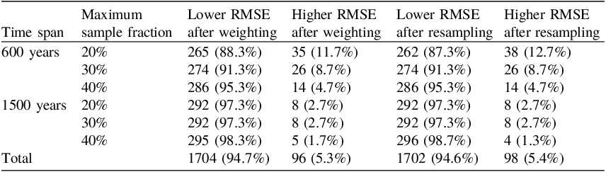


 Li(t)
Li(t) Pi(t)
Pi(t) Wi(t)
Wi(t) Ri(t)
Ri(t)


 Open access