





1. Introduction
Time-lapse cameras are often used to study dynamic environmental changes in remote areas (Brinley Buckley and others, Reference Brinley Buckley, Allen, Forsberg, Farrell and Caven2017; Winterl and others, Reference Winterl, Richter, Houstin, Nesterova and Bonadonna2020; Bongio and others, Reference Bongio, Arslan, Tanis and De Michele2021; Grenier and others, Reference Grenier, Decaulne and Bhiry2022). Some of the most prominent examples are processes of glacier ablation, landslides and coastal erosion events (van der Werff and others, Reference van der Werff, Meijde and Shafique2018; Pintado and Jackson, Reference Pintado and Jackson1106; Xin and others, Reference Xin, Pu, Liu and Liu2023; Dematteis and others, Reference Dematteis, Troilo, Scotti, Colombarolli, Giordan and Maggi2024). Here, we focus on the application of time-lapse imagery for studying iceberg calving—a process defined as a mechanical loss of ice from the marine margins of tidewater glaciers and ice shelves (e.g., van der Veen, Reference van der Veen1996; Benn and others, Reference Benn, Warren and Mottram2007). Calving combined with submarine melting defines the frontal ablation of marine-terminating glaciers (MTGs) (Alley and others, Reference Alley, Anandakrishnan, Christianson, Horgan, Muto and Parizek2015; Shepherd and others, Reference Shepherd, Ivins, Rignot, Smith, van den Broeke and Velicogna2020); however, determining the exact contribution of these two processes to overall ice loss is complicated (Motyka and others, Reference Motyka, Hunter, Echelmeyer and Connor2003; Straneo and Cenedese, Reference Straneo and Cenedese2015). As recently demonstrated by Wood and others (Reference Wood2021), the difficulty in incorporating realistic ice/ocean interactions in numerical simulations may lead to underestimates of the ice loss from Greenland by at least a factor of 2; one of the major reasons behind this issue is the complexity of the calving process.
1.1. Marine-terminating glaciers ice loss mechanics
The terminus position of an MTG is governed by the balance between mass loss through calving and melt (collectively referred to as frontal ablation) and the ice flux into the terminus region. Calving occurs when chunks of ice break off due to stress, buoyancy and melting at the ice-ocean interface (e.g., Post and others, Reference Post, O’Neel, Motyka and Streveler2011). This dynamic process maintains a state of equilibrium, though external factors like ocean warming and climate change can disrupt it, leading to accelerated retreat. During the colder months, snowfall accumulates and is compacted into ice, forming a cyclical process that is mostly in equilibrium (Motyka and others, Reference Motyka, Hunter, Echelmeyer and Connor2003; Mallalieu and others, Reference Mallalieu, Carrivick, Quincey and Smith2020). However, for a significant number of MTGs, this balance has been lost during the past few decades. The factors influencing the occurrence of calving events are not yet fully understood (Sikonia, Reference Sikonia1982; Zhu and others, Reference Zhu2024). One of the most common mechanisms by which iceberg calving events are explained is that warmer temperatures (during the summer season) cause ice in the glacier to melt, creating a warm stream that flows towards the glacier terminus. These streams, known as meltwater plumes, undercut the ice front of the glacier creating a structural weakness, allowing ice to fall (How and others, Reference How2019).
Calving rates and styles change greatly in space (geographically and along the glacier terminus) and time (daily and seasonal fluctuations and long-term trends). For example, ice shelves in Antarctica calve massive ( $\sim$10 $^6$ m $^3$) icebergs at multi-year intervals (e.g., MacKie and others, Reference MacKie, Millstein and Serafin2024), while typical calving rates at many tidewater glaciers in Greenland, Svalbard and Alaska reach hundreds of small-magnitude ( $\sim$10 $^3$ m $^3$) events per day (e.g., Bartholomaus and others, Reference Bartholomaus, Larsen, West, O’Neel, Pettit and Truffer2015); How and others (Reference How2019); Cook and others (Reference Cook, Christoffersen, Truffer, Chudley and Abellán2021). Moreover, a large heterogeneity of the calving flux has been observed along the termini of glaciers in Alaska (Wagner and others, Reference Wagner2019) and Greenland (Kneib-Walter and others, Reference Kneib-Walter, Lüthi, Funk, Jouvet and Vieli2023). Glaciers calve as a result of various mechanisms: longitudinal stretching, buoyancy forcing and melt undercutting (e.g., van der Veen, Reference van der Veen1996); Benn and others (Reference Benn, Warren and Mottram2007). Consequently, there are numerous drivers that influence calving rates and styles, including but not limited to the ice velocity, air and water temperature, precipitation, solar radiation, grounding depth and amount of ice mélange buttressing the terminus (e.g., van der Veen, Reference van der Veen1996; Benn and others, Reference Benn, Warren and Mottram2007; Luckman and others, Reference Luckman, Benn, Cottier, Bevan, Nilsen and Inall2015; How and others, Reference How2019; Mallalieu and others, Reference Mallalieu, Carrivick, Quincey and Smith2020; Ciepły and others, Reference Ciepły2023). Recent research (Kochtitzky and others, Reference Kochtitzky, Copland and Van Wychen2022) has confirmed that the spatial distribution of frontal ablation plays a pivotal role in determining the total mass balance of tidewater glaciers. The authors of the paper quantified frontal ablation across Northern Hemisphere MTGs using satellite observations from 2000 to 2020, revealing that frontal ablation—comprising both calving and submarine melt—accounts for approximately two-thirds of the total ice discharge from the region. Their results demonstrated substantial spatial variability, with regions of high calving fluxes coinciding with dynamically fast-flowing outlet glaciers. Additionally, it was observed that in all analysed regions there are some glaciers that contribute disproportionately to that loss and some that are more stable. Large spatio-temporal variability, the occurrence of different styles and the diversity of driving factors make it extremely challenging to study and fully understand calving based solely on satellite remote sensing. Different techniques are used to overcome the limitation associated with the analysis of iceberg calving with satellite image processing; examples include terrestrial laser scanning and radar interferometry (e.g., Pętlicki and Kinnard, Reference Pętlicki and Kinnard2016; Walter and others, Reference Walter, Lüthi and Vieli2020), passive cryoseismology and cryoacoustics (e.g., Podolskiy and Walter, Reference Podolskiy and Walter2016; Glowacki and Deane, Reference Glowacki and Deane2020) and observation of calving-driven mini-tsunami waves (Minowa and others, Reference Minowa, Podolskiy, Jouvet, Weidmann, Sakakibara and Tsutaki2019). However, these remote sensing techniques usually require specialised (and often very expensive) technology and high qualification of the user in terms of data collection and analysis (O’Neel and others, Reference O’Neel, Marshall, McNamara and Pfeffer2007a).
1.2. Time-lapse images acquisition and manual processing
Despite the inherent challenges of conducting research in remote areas, time-lapse images of glaciers have been collected since the late 1960s (Medrzycka and others, Reference Medrzycka, Benn, Box, Copland and Balog2016; Minowa and others, Reference Minowa, Podlasky, Sugiyama, Sakakibara and Skvarca2018) to improve understanding of glacier dynamics. The high sampling rate and resolution of this type of monitoring, compared with satellite imagery, enable the detection of smaller calving events and observations over much shorter timescales. The first pioneering studies focused on measuring ice velocities (Flotron, Reference Flotron1973; Krimmel and Rasmussen, Reference Krimmel and Rasmussen1986), but subsequent technical developments allowed more frequent image capture and, consequently, the observation of individual calving events at tidewater glaciers. The decline in camera costs and improvements in image quality have made this method of observation increasingly common. However, manual labelling (in computer vision, labelling involves marking specific features or elements within visual data and associating them with predefined classes or attributes, which are then used as training or validation data) of calving events from time-lapse imagery remains a time-consuming process, further complicated by the large volumes of data collected.
The use of time-lapse cameras for analysing and detecting calving events is limited by a few factors. It is usually impossible to constantly monitor camera operation due to lack of internet connection or LoRaWAN (Long Range Wide Area Network) network limitations. Lack of communication with the camera means it is not possible to intervene when a technical problem occurs, which can lead to a loss of data. Challenges include technical issues with powering, clock drift and unwanted movements caused by strong winds or animals; small changes in camera orientation may translate to large errors in estimates of location and size of real objects (Carvallo and others, Reference Carvallo, Llanos, Noceti and Casassa2017). In addition, variable weather and lighting conditions impact the usability of images; examples include the amount of sunshine, precipitation and the occurrence of the polar night. The system needs to be designed to operate without monitoring, and the user should be prepared for the possibility that data might not be retrievable. This is why many datasets cover only short periods of time, one season or part of it. Nevertheless, time-lapse cameras placed in remote areas typically capture at much higher temporal resolutions than satellite imagery but are still rarely at intervals shorter than 15 min, and, when they do, it is often for very limited durations (Minowa and others, Reference Minowa, Podlasky, Sugiyama, Sakakibara and Skvarca2018) and often for very specific applications. This, similarly as before, is due to the capacity of the memory cards and batteries and lack of maintenance on site that would ensure the long-life of the system (Medrzycka and others, Reference Medrzycka, Benn, Box, Copland and Balog2016). However, there are some notable long-time image time-lapse datasets (Welty and others, Reference Welty, O’Neel and Pfeffer2012; Moskalik and others, Reference Moskalik, Głowacki and Luks2022) available for the general public to use.
A few prominent examples of studies based on more frequently taken images have been conducted. For example, How and others (Reference How2019) analysed high-frequency (3 s intervals) time-lapse images of the terminus of Tunabreen in Svalbard to relate calving activity to different environmental factors, including air temperature, location of subglacial plumes, periodic changes in sea surface height (tidal cycle) and spatially varying ice velocity and bathymetry. The image analysis revealed patterns undetectable by satellite imagery, showing that most calving events occurred on the falling limb of the tide and were concentrated at or above the waterline. Similarly, calving rates and styles have been investigated with time-lapse imagery in many other regions where glaciers flow to the water; examples include Greenland (Kneib-Walter and others, Reference Kneib-Walter, Lüthi, Funk, Jouvet and Vieli2023), Alaska (O’Neel and others, Reference O’Neel, Echelmeyer and Motyka2003), Iceland (Tinder, Reference Tinder2012), Patagonia (Minowa and others, Reference Minowa, Podlasky, Sugiyama, Sakakibara and Skvarca2018) and Antarctica (Banwell and others, Reference Banwell2017). In several studies, time-lapse images were used to calibrate acoustic, seismic and other remote sensing techniques intended for long-term and continuous monitoring of calving (e.g., O’Neel and others, Reference O’Neel, Marshall, McNamara and Pfeffer2007b; Glowacki and others, Reference Glowacki, Deane, Moskalik, Blondel, Tegowski and Blaszczyk2015; Köhler and others, Reference Köhler, Pętlicki, Lefeuvre, Buscaino, Nuth and Weidle2019; Minowa and others, Reference Minowa, Podolskiy, Jouvet, Weidmann, Sakakibara and Tsutaki2019). Manual detection of calving events requires great effort in comparing image pairs; processing thousands of images from a single season (glacier cycle) may take weeks or even months. For this reason, the creation of automatic algorithms for image processing has become important to the glaciological community and is the main focus of this study.
1.3. Automatic pipelines for calving detection
Even if taking into account the difficulties with image acquisition described above, the pure volume of the images obtained and the varying quality of them make it hard to analyse data by manually sorting through them. This is why even though a large number of short-term analyses are being done manually (Glowacki and others, Reference Glowacki, Deane, Moskalik, Blondel, Tegowski and Blaszczyk2015; Messerli and Grinsted, Reference Messerli and Grinsted2015; Kneib-Walter and others, Reference Kneib-Walter, Lüthi, Moreau and Vieli2021). One of the large issues frequently observed with glacier time-lapse images is significant difference in light conditions or weather conditions leading to neighbouring images being significantly different in appearance (Vanrell and others, Reference Vanrell, Lumbreras, Pujol, Baldrich, Llados and Villanueva2001; Riabchenko and others, Reference Riabchenko, Lankinen, Buch, Kämäräinen and Krüger2013; Lymer, Reference Lymer2015). There are various methods available in the computer vision community (Buchsbaum, Reference Buchsbaum1980; Finlayson and others, Reference Finlayson, Schiele and Crowley1998) including comprehensive image normalisation algorithm that works by iteratively applying normalisation to the RGB channels until subsequent applications have no further effect. In environmental studies, unusable images are often automatically detected using criteria such as histogram analysis, image sharpness or colour count. Some attempts at establishing thresholds for the mean and standard deviation of colour distribution in specific image regions to identify low-visibility conditions have been made (Gabrieli and others, Reference Gabrieli, Corain and Vettore2016). In some cases, this is being done by textural features (Hadhri and others, Reference Hadhri, Vernier, Atto and Trouvé2019) or by RGB histograms (Lenzano and others, Reference Lenzano, Lannutti, Toth, Rivera and Lenzano2018). Authors employed a support vector machine to classify images based on visibility conditions and lighting type (direct or diffuse) (Lenzano and others, Reference Lenzano, Lannutti, Toth, Rivera and Lenzano2018).
In this section, we are going to describe calving events detection pipelines that base on vision data. Satellite-based iceberg detection studies vary between using data for counting already-calved icebergs originating from large glaciers (Podgórski and Pętlicki, Reference Podgórski and Pętlicki2020) using CNN (convolutional neural networks) to classify between glacier calving front icebergs and ice mélange (Marochov and others, Reference Marochov, Stokes and Carbonneau2021) or detection of glacier calving margins (Mohajerani and others, Reference Mohajerani, Wood, Velicogna and Rignot2019). How and others (Reference How2019) present an automatic way to detect calving events basing on ground-based time-lapse images. Other studies using ground-based images allow to detect the areas on the front when calving has occurred and to measure the volume (,103), Adinugroho and others, Reference Adinugroho, Vallot, Westrin and Strand2015. In particular, Vallot and others (Reference Vallot2019) method involved segmenting the glacier front from the rest of the glacier, detecting changes between both images and producing a mask to detect the calving region. While this method was shown to work well when the weather was favourable, it performed poorly when fog or high illumination was present in the images. This resulted in only 55% of test images being deemed usable hence missing a large number of calving events. The method relies on several carefully chosen parameters that are specific to the data meaning that it is not easily adaptable to a wider context. The quality of images captured in polar regions can vary significantly due to harsh weather conditions, necessitating preprocessing of the data and the removal of unusable images before analysis. Common issues affecting image quality include dense fog, low illumination angles and precipitation on the lens.
Environment change detection algorithms aim to detect any differences to the subjects in an image in reference to another image. Hussain and others () discussed a technique to detect changes across images, which involves comparing the pixel intensity values across frames to produce a residual image of changes and counting the number of pixels with changes. If the difference is greater than a particular threshold, we consider there to be a change. Selecting a suitable threshold is not easy and requires multiple values to be evaluated for accuracy. This method does not consider the spatial correlation between neighbouring pixels and requires both images to be very accurately aligned Brown ().
In this paper, we present a computer vision based method to filter out images rendered unusable due to weather effects such as fog and precipitation by calculating the number of salient key-points (distinct, invariant image features) detected in the image using the SIFT (Scale-Invariant Feature Transform) algorithm as an indicator of the visibility of the glacier front and discarding any image with fewer key-points than a defined threshold. We propose the use of SNN (Siamese neural network) and show that it is useful in detecting calving events since it allows to separately calculate features on two images and then merges them together in order to track differences between them thus detecting calving areas.
2. Methodology and implementation
2.1. Dataset selection
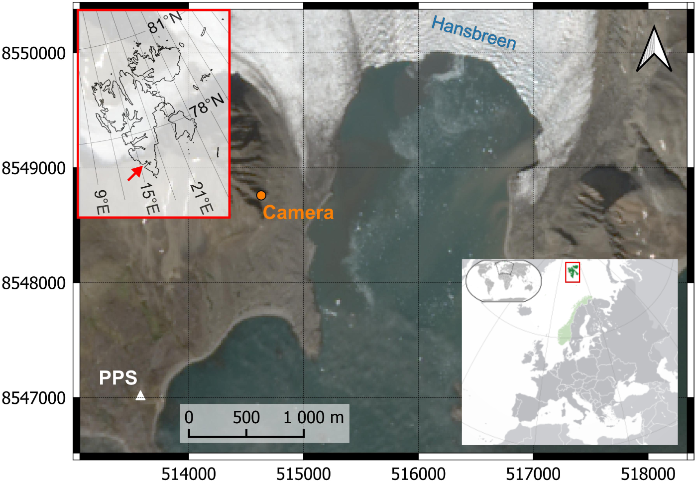
The time-lapse imagery used in this paper is of Hansbreen (Moskalik and others, Reference Moskalik, Głowacki and Luks2022), located in the Norwegian archipelago of Svalbard and was collected by the Polish Polar Station in Hornsund. Hansbreen has retreated by more than 2.7km since the end of the 19th century (Oerlemans and others, Reference Oerlemans, Jania and Kolondra2011). The dataset used in this study was acquired at 15 min intervals, yielding slightly fewer than 3000 images per month during the summer, when the sun does not set. Illumination differences between consecutive frames, resulting from changes in solar position and cloud cover, as well as environmental factors such as wind or occasional camera adjustments to improve glacier coverage, introduced minor displacements of the camera over longer time intervals.
The images were captured between 2015 and 2022 at 15 min intervals as part of the station’s monitoring programme. To simplify evaluation, we focused on a small subset of data and selected the images captured in July of 2016. The summer months experience a higher number of calving events and feature more favourable weather. This time range also provides a better viewpoint of the glacier, which has retreated significantly since 2020, causing the camera setup to be positioned further away from the glacier terminus.
As this paper presents a method for detecting calving events from this and similar datasets, we used a representative sample to demonstrate data preparation, pipeline construction and expected accuracies. We introduce a method for detecting significant ice loss from the glacier front between two consecutive images. The methods developed here are designed to be applicable to the remaining dataset with minimal modification.
Location of the study site and the time-lapse camera. Hansbreen location in relation to the Svalbard archipelago. The coordinate system used for the detailed map frame is UTM coordinates, WGS84 datum, Zone 33N (EPSG:32633), while the coordinate system used for the general Svalbard map is geographic coordinates.

2.2. Dataset pre-processing
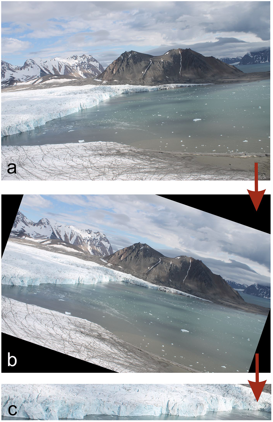
The images in the dataset captured a large landscape with mountains in the background and a bay at the front of the glacier. The glacier covered less than half of the image so the image would have to be cropped such that only the glacier front which is of interest in this paper would be seen. Rotation to align the waterfront to be horizontal would also have to be performed. This is done to ensure consistent perspective through all the pictures (see Fig. 2). These transformations were applied as a batch to all the images in our dataset with simple manually chosen parameters. For example, the July 2016 dataset was cropped from 4272 $\times$2848 pixels to 2000 $\times$270 pixels with a clockwise rotation of 19 degrees. Iceberg calving causes ice loss and the glacier front to retreat over time; hence, the images would have to be cropped in such a way that all the images in the batch would fit within the selected region. A more dynamic approach that crops and rotates the image based on an extracted mask (such as U-Net) of the glacier could have been deployed but this was not deemed necessary as re-calibration of parameters would only be required once per month (every 2880 images for 30 days, 2976 images for 31 days).
Transformations applied to the original image to extract the area of interest. (a) Original image sized 4272 $\times$2848 pixels. (b) Image rotated by 19 degrees clockwise. (c) Image rotated by 19 degrees followed by cropping to 2000 $\times$270 pixels.

2.3. Selection of usable images
An important barrier that needed to be overcome before attempting to automatically detect calving events was the filtering of any images where the glacier front was completely occluded or only partially visible, making it impossible to compare images.
In order to evaluate candidate solutions for filtering out unusable images, we first established a benchmark by manually labelling a subset of our data. Labelling was performed with a web-based image annotation tool named Computer Vision Annotation Tool (CVAT) (CVAT.ai Corporation, 2022). Using CVAT, we tagged images based on whether they were deemed usable with a substantial part of the glacier front being visible. 698 images out of the 2653 images in the dataset were labelled by this procedure. 627 images were labelled as usable, 32 as unusable and 39 as partially usable, meaning approximately 90% of the images were classified as usable. The number of usable images is expected to be much lower for other months with harsher weather conditions, further indicating the need for an automated procedure.
To frame the task as a binary classification problem, 39 partially usable images were excluded from the dataset. The remaining 659 labelled images were randomly divided into training and test subsets using an 80:20 split, which was selected as an appropriate balance between model learning capacity and reliable performance evaluation. The training subset was used during the model development phase, while the test subset served to assess performance on previously unseen data. Care was taken to ensure that the proportion of usable images in both subsets closely reflected that of the complete dataset, thereby maintaining representative data distribution.
We used SIFT algorithm which detects salient key-points in an image such as edges and high contrast points (Pratt, Reference Pratt1974; Lowe, Reference Lowe2004). When the glacier was visible and under normal lighting conditions, it would portray a large number of key-points due to the texture of the ice that could be identified by SIFT. The number of feature descriptors in an image was found to be a very good indicator of the visibility of the glacier as dense fog and harsh illumination would reduce the number of visible edges that could be detected. By this measure, we could compute and count the number of feature descriptors for each image and discard any images that had fewer key-points than a threshold.
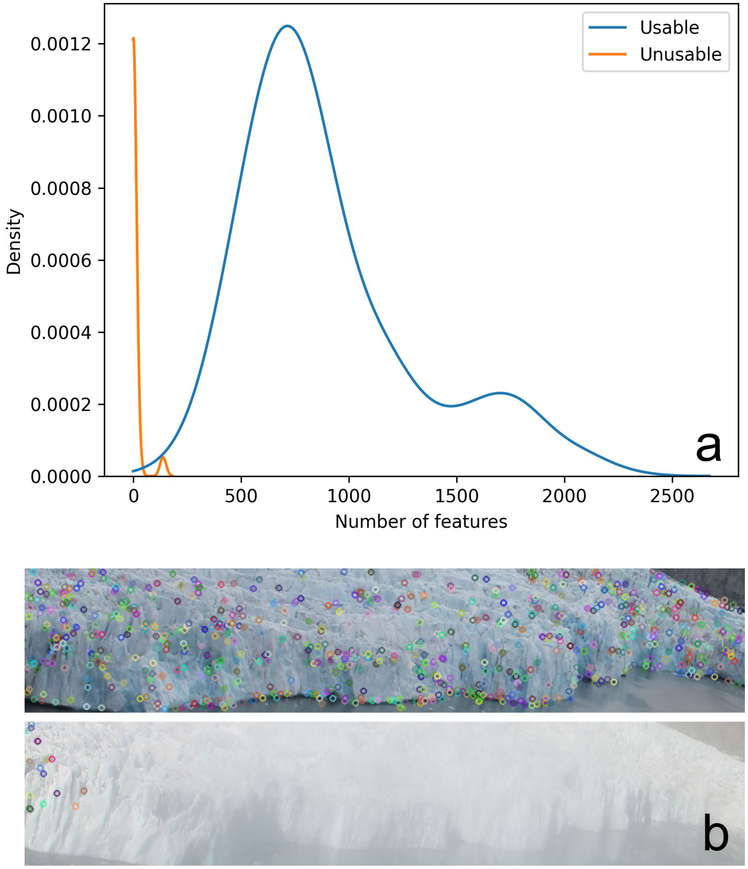
By plotting the number of key-points for usable and unusable images in the training dataset, as shown in Fig. 3, we see that they follow a pattern similar to Gaussian distribution. Usable images have a mean of 901 key-points, a standard deviation of 418 and a minimum of 54. The mean number of key-points for unusable images is six with a standard deviation of 27. Using this information, we determined 50 to be a suitable threshold for the minimum number of key-points to classify an image as usable.
SIFT key-points of images in the training dataset, (a) distribution of the number of SIFT key-points for usable and unusable images in the training dataset, (b) SIFT key-points of a usable image (top) and unusable image (bottom).

2.4. Calving detection for image pairs
Calving events also needed to be manually identified and annotated in the dataset for the purpose of evaluating our automated calving detection model. CVAT allowed us to compare subsequent image pairs and draw annotated boxes denoting calving locations. We labelled a total of 650 image pairs, with 72 displaying change and 578 showing none. Iceberg calving smaller than 50 $\times$50 pixels (representing about 0.5% of the 2000 $\times$270-pixel glacier front) were ignored as these were considered too small. Using a larger dataset that includes smaller calving events would require additional computation time and the use of a GPU cluster, which was not considered necessary at the experimental stage. As with the dataset used for detecting image usability, this dataset was randomly split into training and testing sets with an 80:20 ratio. Since the dataset is imbalanced, we verified that the split maintained approximately the same proportion of the two classes as the overall dataset.
2.4.1. Network architecture
CNNs are a type of neural network that works by applying a transformation using a convolution kernel to a small region of the image matrix defined by the kernel size (Krizhevsky and others, Reference Krizhevsky, Sutskever and Hinton2017). The kernel slides across the matrix, applying the transformation to that region. The resulting output is a feature map capturing edges and shapes in the input. Typically, a few convolutional layers are used in succession, followed by fully connected linear layers for image classification models such as the VGG model presented by Simonyan and Zisserman (), which was trained on the ImageNet dataset—a large public image repository with more than 14 million annotated images that is commonly used as a benchmark for classification model accuracy. The VGG model was also shown to generalise well to other datasets with minor modifications (Krizhevsky and others, Reference Krizhevsky, Sutskever and Hinton2017). We advocate the use of handcrafted (SIFT) key-points for detecting usable images because this is a straightforward task where we know in advance that blob-like features are indicative of a sharp image. However, for the more challenging and fine-grained task of calving detection, we believe a modern end-to-end machine learning based approach is required. Hence, we decided to use a modified version of VGG as a basis for our model.
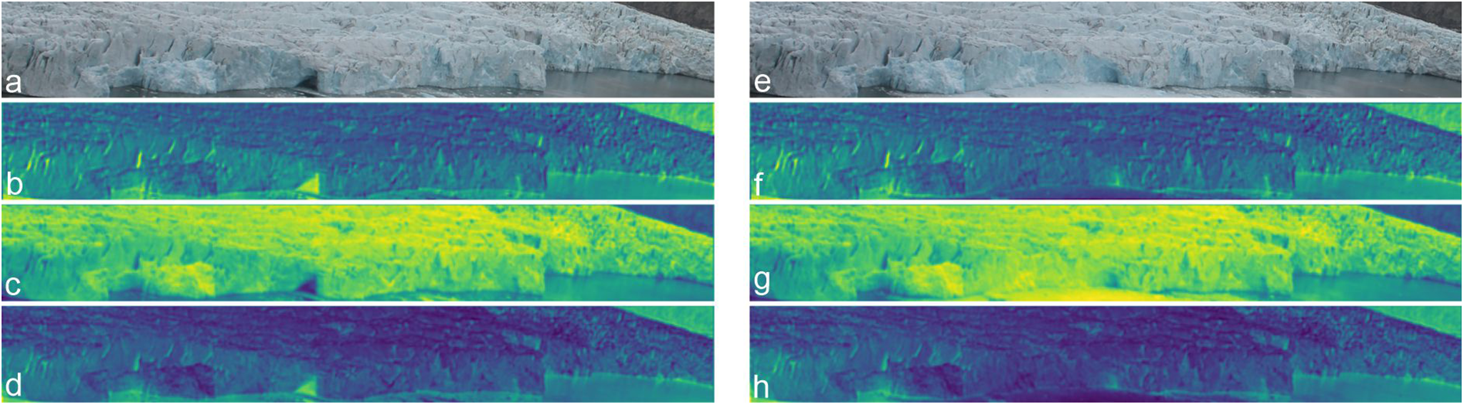
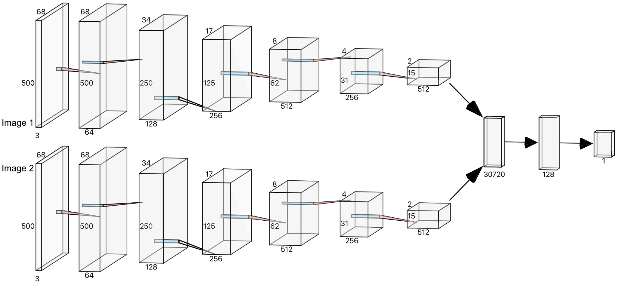
We chose to calculate the feature maps produced by the convolutional layers for each image in the pair and create a model to detect iceberg calving events by evaluating differences in the feature maps (see Fig. 4). As the model would have to take two inputs, a traditional classifier neural network architecture with one input and a number of outputs corresponding to the number of classes would not be adequate for our problem. But SNN (see Fig. 5) is a type of network architecture where two inputs are passed into the same network and their outputs are compared using a similarity function, typically the Euclidean distance (Bromley and others, Reference Bromley, Guyon, LeCun, Säckinger, Shah, Cowan, Tesauro and Alspector1993). We opted to use an adapted version of an SNN by passing both images through the convolutional layers of the VGG model, which are generalised to detect abstract features, while discarding the subsequent fully connected layers. The feature maps of both images are combined to form the input of two new fully connected layers with 30,720 inputs and one output. This model is a binary classifier where the output indicates whether the input image pair contains a calving.
Comparison of the original images (a) and (e) and feature maps (b)-(f) (c)-(g) (d)-(h) generated by the first layer of the VGG network for a pre-calving (b)(c)(d) and post-calving image (f)(g)(h) pair. The visualised feature maps are for the first three learned filters in the first VGG layer.

Siamese neural network architecture where VGG feature maps are computed separately for each input image and then combined as the input for linear layers to output a binary value indicating the occurrence of a calving event in the image pair.

Before the images were added into the network, they were resized such that the width and height were reduced by 75% to an image sized 500 $\times$68 pixels. This reduced the model complexity while preserving the image ratio and allowing key image features to remain visible (Vanrell and others, Reference Vanrell, Lumbreras, Pujol, Baldrich, Llados and Villanueva2001). Since we use pretrained convolutional layers from the VGG model, our input images must be normalised consistently with how the original training data for VGG was prepared. Accordingly, we first rescale the pixel intensity values from the range $0$–
$0$– $255$ to $0$–
$0$– $1$. We then subtract the mean of the VGG training data ( $R = 0.485$, $G = 0.456$, $B = 0.406$) to mean-centre the images, followed by division by the corresponding standard deviations ( $R = 0.229$, $G = 0.224$, $B = 0.225$), ensuring that the input intensities follow a standard normal distribution. The convolutional layers produced 512 features each with a size of $15\times2$ pixels. These features were flattened into a vector sized 15360 for each image in the pair and then combined together to form a vector of size 30720 before being used as inputs for the fully connected layers.
2.4.2. Data augmentation and class imbalance
Data augmentation techniques have been shown to greatly improve a model’s ability to generalise to unseen data (Shorten and Khoshgoftaar, Reference Shorten and Khoshgoftaar2019). Given the low amount of data and the significant class imbalance of calving events only composing 9% of the training dataset, it was necessary to take appropriate steps to mitigate the model overfitting to the majority data class. Specifically, we used weighted random sampling such that images were randomly chosen with probabilities proportional to the inverse of the class frequencies. This means that the minority calving class images were over-sampled. In order to ensure sufficient diversity in the over-sampled class and to avoid overfitting, we use data augmentations. Specifically, we used random horizontal flipping with  $p=0.5$, random perspective distortion with distortion scale 0.2 and $p=0.5$ and random rotations chosen uniformly from $\pm 6^\circ$. Additionally, images were paired across larger timescales to increase the number of pairs showing a calving event.
2.4.3. Model training
The loss function is used to evaluate how close the predicted value from a model is to its true value. Higher loss values indicate that the predicted value is further away from its true value. During training, the loss of the prediction is calculated and the parameters are adjusted, using backpropagation, to minimise the loss (Zaras and others, Reference Zaras, Passalis, Tefas, Iosifidis and Tefas2022).
The chosen loss function ( ${L}_{bce}(y, \hat{y})$ ) for training the model was the Binary Cross Entropy loss, which is often used for binary classification. This can be described by the following equation $\mathcal{L}_{bce}(y, \hat{y})=-{(y\log(\hat{y}) + (1 - y)\log(1 - \hat{y}))}$ where $y$ is the true value and $\hat{y}$ is the predicted value. It penalises predictions based on their confidence and the difference to the true value. For example, a high confidence positive class prediction with a true negative class, would be penalised more than a low confidence positive class prediction.
The Adam optimiser (Kingma and Ba, Reference Kingma and Ba2014) is an extension of the classical Stochastic Gradient Descent (SGD) algorithm that introduces adaptive learning rates for each parameter based on the magnitude of recent gradients. This means that the algorithm is less sensitive to noisy gradients through the use of momentum, and it has been shown to converge to optimal solutions faster than SGD. The model was trained using  $batch\ size=4$ and the Adam optimiser with the hyper-parameters $learning\ rate = 3\times10^{-4}$, $\beta_1=0.9$ and $\beta_2=0.999$, chosen after experimentation with various values. The learning rate dictates the step size that the optimiser takes to update weights. Large learning rates can cause the optimiser to overshoot the optimal solution, while small learning rates lead to slow convergence. The $\beta$ values are used to compute the running averages of gradients. During each epoch, the dataset is divided into batches, each containing a number of samples equal to the batch size, which are used iteratively optimise the model. Small batch sizes require less memory, however they can cause slow convergence rates. Large batch sizes require more memory and can lead to overfitting. Choosing appropriate hyper-parameters is essential to train a model to achieve good accuracy. The final architecture is shown on Fig. 5.
We leveraged transfer learning methods to use pre-trained weights of a VGG model trained on a subset of the ImageNet dataset. This is an approach that has been shown to reduce training times and the size of the training dataset (Weiss and others, Reference Weiss, Khoshgoftaar and Wang2016). We removed the final classification layer using the remaining layers as a pre-trained features extractor. We froze the weights of all of these layers and added two fully connected layers. During training only the weights of the new fully connected layers were trained. By ‘weights’ we refer to the adjustable parameters of the CNN model that must be learned in order to minimise the training loss. The number of parameters corresponds to the complexity of the model and its capacity to fit the data. However, when the model is too flexible (i.e., has too many parameters), it can overfit the training data and fail to generalise well to unseen data. In total, the network contained 13 152897 parameters but only the 3 932417 parameters in the fully connected layers needed to be optimised.
The model was developed and trained on an Apple MacBook Pro with an M2 Pro GPU and the Metal Performance Shaders backend, which provided faster training compared to CPU-only processing. Training was performed over 10 epochs, with the entire dataset processed once per epoch. After each epoch, the loss and accuracy were evaluated on the test dataset and the model from the epoch with the highest accuracy was chosen as the candidate solution.
2.5. Tooling
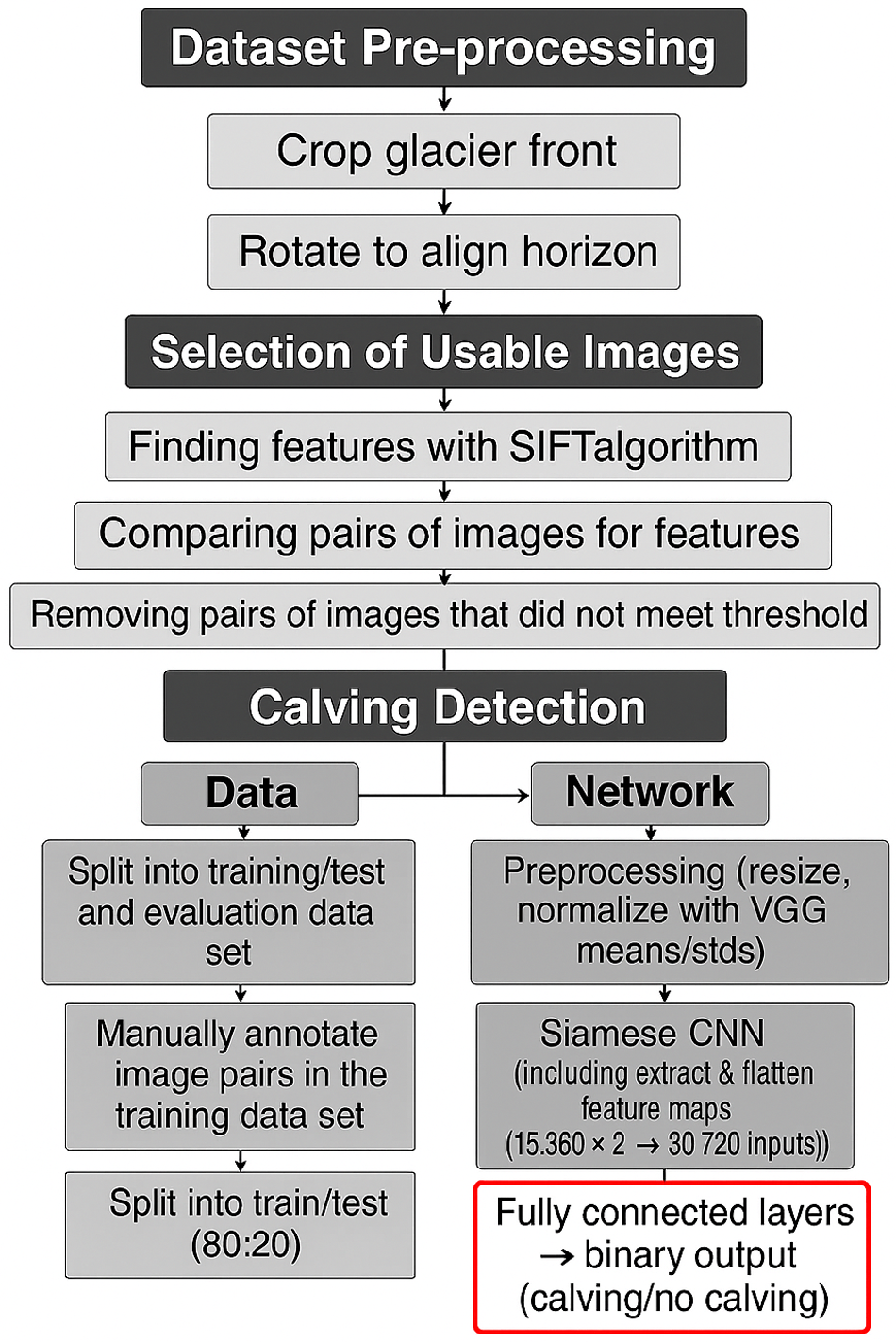
All of the code used in the paper was written in Python. Image pre-processing and SIFT keypoint extraction were performed using the CV2 library (Bradski, Reference Bradski2000). The neural network was implemented in PyTorch (Paszke and others, Reference Paszke, Gross, Massa, Lerer, Bradbury, Chanan, Wallach, Larochelle, Beygelzimer, d’Alché Buc, Fox and Garnett2019), which provided an intuitive interface and GPU acceleration to reduce training time. Figure 6 shows the final workflow of the pipeline used in this project.
The workflow of the final data processing pipeline.

2.6. Evaluation metrics
The performance of the two presented methods in this paper: (i) classification of usable images and (ii) detection of calving events from a pair of images–will be evaluated on both training and testing datasets using a range of standard metrics. To assess the method’s generalisability, we will also apply it to data from other time periods. Additionally, we will examine failure cases to better understand the limitations of the approach.
In order to understand how the model’s classification accuracy varies for each class, we will use a confusion matrix (Abeysinghe and others, Reference Abeysinghe, Welivita and Perera2019). Confusion matrices compare the predicted and true labels and display the number of correct and incorrect predictions for each class (see Fig. 11). Table 1 shows the template for a confusion matrix of a binary classification model. The values on the confusion matrix can also allow us to calculate other useful metrics.
Confusion matrix for binary classification used to illustrate the performance of the prediction model.

The  $F_1$ score is a metric that considers the harmonic mean of precision and recall. Precision is the proportion of true positive predictions to the total number of positive predictions, while recall is the proportion of true positive predictions to the total number of actual positives. The $F_1$ score provides a balanced measure that accounts for both false positives and false negatives:
 \begin{equation}
F_1 = \frac{2*Precision*Recall}{Precision+Recall} = \frac{2*TP}{2*TP+FP+FN},
\end{equation}
\begin{equation}
F_1 = \frac{2*Precision*Recall}{Precision+Recall} = \frac{2*TP}{2*TP+FP+FN},
\end{equation} where TP, FP and FN are defined as in Table 1. To understand the correlation between two variables, Pearson’s correlation coefficient can be calculated between them (see Fig. 9). The value ranges between -1, indicating a very strong negative correlation and 1, indicating a very strong positive correlation. 0 indicates that there is no correlation between the two variables. The formula for the rank coefficient between samples  $X$ and $Y$ each containing $n$ values with means $\overline{x}$ and $\overline{y}$ is given in Equation 2.
 \begin{equation}
r = \frac{{}\sum_{i=1}^{n} (x_i - \overline{x})(y_i - \overline{y})}{\sqrt{\sum_{i=1}^{n} (x_i - \overline{x})^2\sum_{i=1}^{n}(y_i - \overline{y})^2}}
\end{equation}
\begin{equation}
r = \frac{{}\sum_{i=1}^{n} (x_i - \overline{x})(y_i - \overline{y})}{\sqrt{\sum_{i=1}^{n} (x_i - \overline{x})^2\sum_{i=1}^{n}(y_i - \overline{y})^2}}
\end{equation}3. Results and analysis
3.1. Evaluation on primary dataset
3.1.1. Selection of usable images
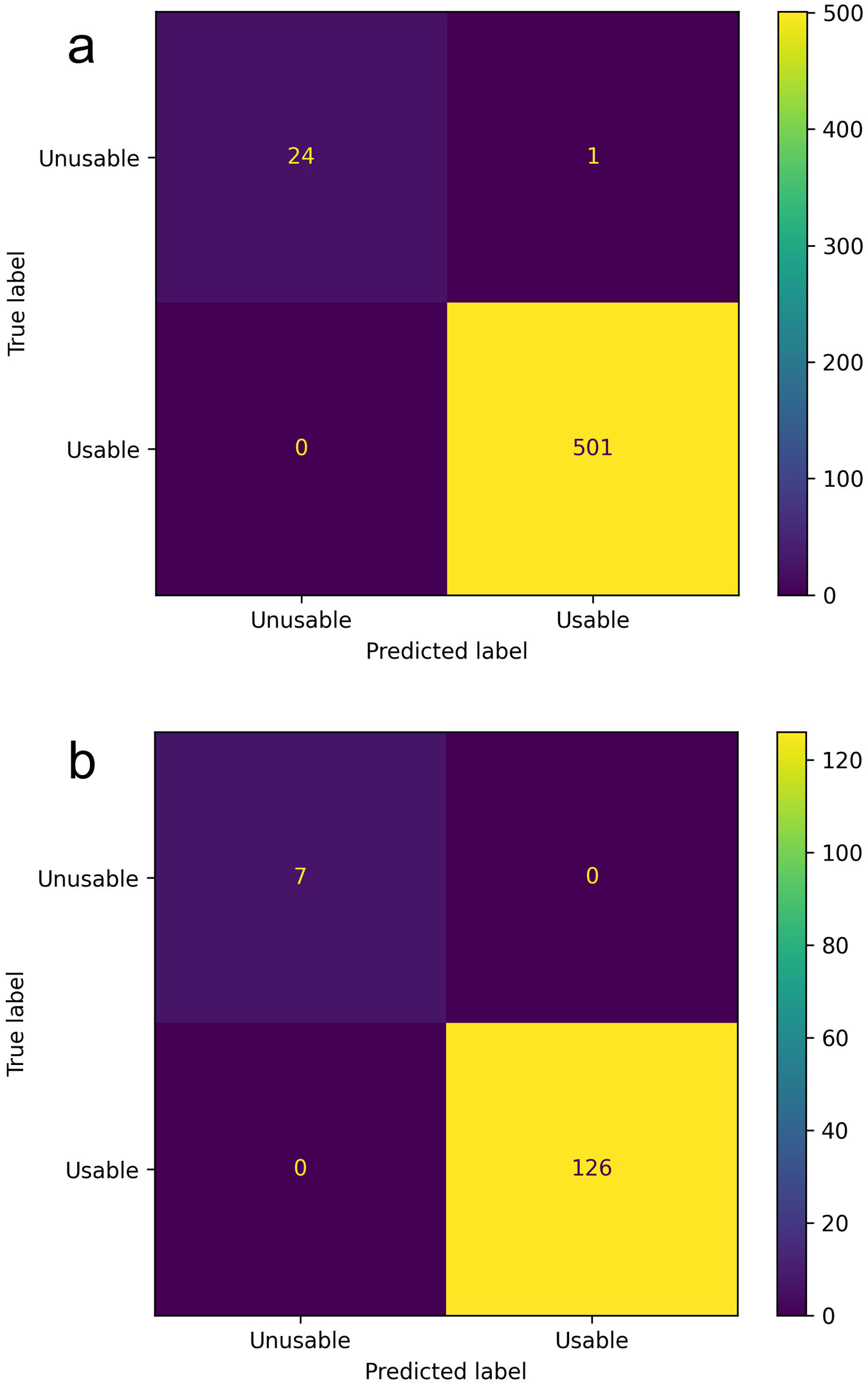
The selected method for classifying usable images achieved an overall classification accuracy of 99.8% on the training dataset with 100% of usable images correctly classified as usable, and 96% of unusable images correctly classified as unusable. On the test dataset, an overall accuracy of 100% was achieved. The selected threshold was able to correctly decide if an image was considered to be usable without any errors. The  $F_1$ score was calculated to be 1.0 for both the training and testing data indicating it is a perfect model on these data (see Fig. 7).
Confusion matrix for usability predictions of July 2016 on the training and testing data. The training data shows an overall accuracy of 99.8% with 100% of usable images correctly classified as usable, and 96% of unusable images correctly classified as unusable. On the test dataset, the model has an overall accuracy of 100%, (a) training data, (b) testing data.

Labelling of image usability was done manually using subjective measures based on significant details from the glacier being visible. This includes some cases with light fog that still allow for some key-points to remain visible. Depending on the required clarity of the glacier front, changing the threshold for the minimum number of key-points provides an intuitive and simple way to achieve this.
3.1.2. Detection of iceberg calving from image pairs
The calving detection model was trained for 10 epochs, and at the end of each epoch, the loss and accuracy on the test data were recorded. Each epoch took about 1 min to run and the training completed in 10 min. The use of transfer learning reduced the number of parameters that would require optimising, and subsequently reduced the training time required to find an optimal solution.
Once training was complete, the parameter weights from the epoch with the best performance on the test data were selected. We considered the percentage of correctly classified non-calving (true negatives) and calving (true positives), and selected the best epoch by weighing up the true positive and true negative accuracies with a ratio of 2:1. The reasoning behind this was that achieving a high accuracy on calving events was deemed to be more important than non-calving events.
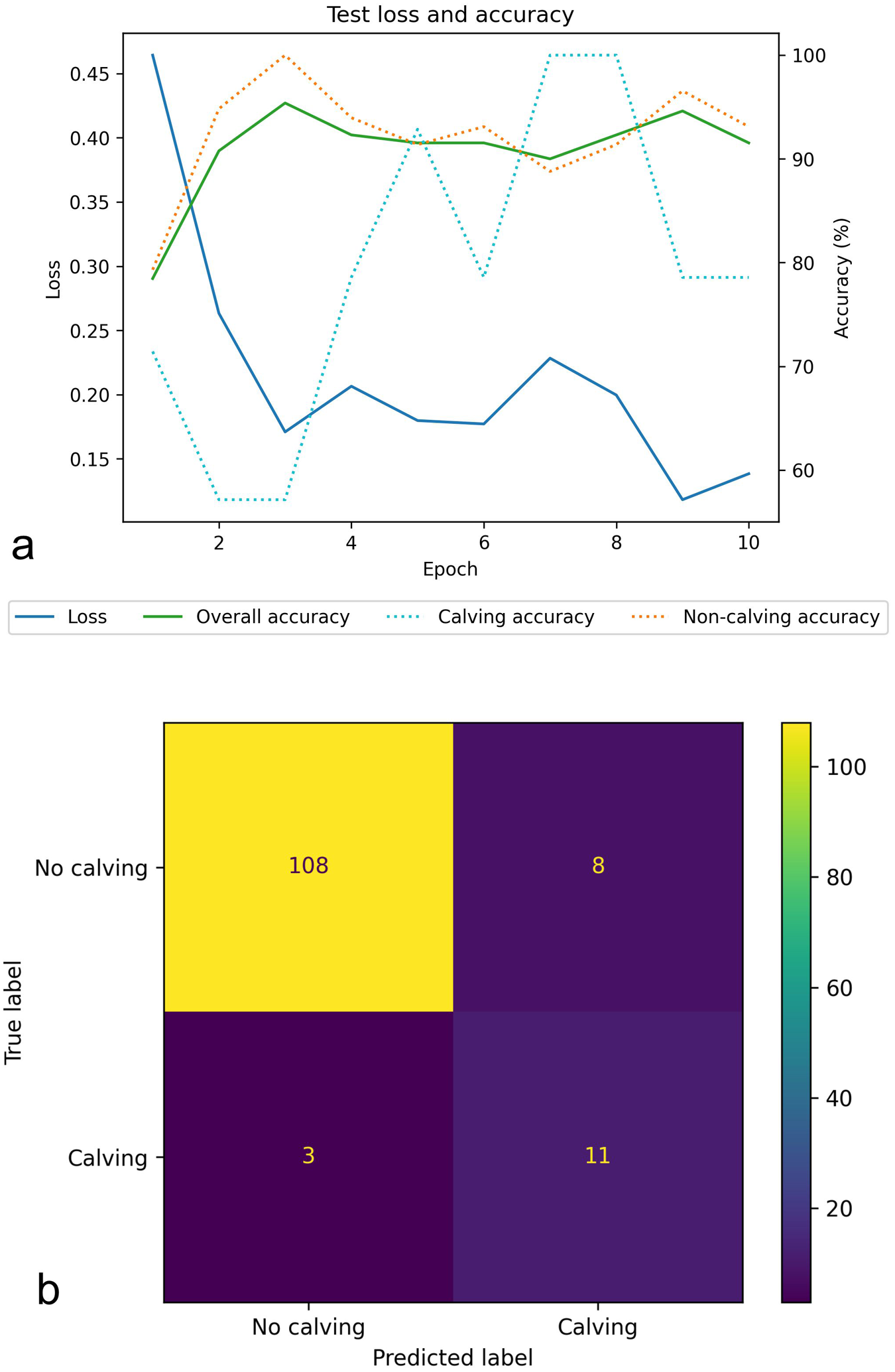
Figure 8(a) shows how the overall accuracy on the training data increased with the number of epochs before converging around 92% at the 3rd epoch and the loss minimised to 0.12 on the 9th epoch. The 8th epoch was chosen to be the candidate solution, based on training data accuracy. This achieved an overall accuracy of 92% on the training data with 100% of calving image pairs and 91% of non-calving pairs being correctly classified. On the unseen test data, the chosen epoch achieved an overall accuracy of 92% with 79% of calving pairs and 93% of non-calving pairs being correctly classified (see Fig. 8). Figure 7 depicts a confusion matrix for the test data, which shows the number of correct and incorrect classifications for each class. The  $F_1$ score on the test data was calculated to be 0.67 indicating that the model overall achieves a reasonable accuracy for classification but it is not a perfect model, with it achieving a much better accuracy on the non-calving image pairs compared to the calving image pairs.
Neural network training performance, (a) loss and accuracy for the training data at the end of each epoch, (b) candidate solution’s confusion matrix of its performance on the test data. The confusion matrix shows an overall accuracy rate of 92% with 79% of calving pairs and 93% of non-calving pairs being correctly classified.

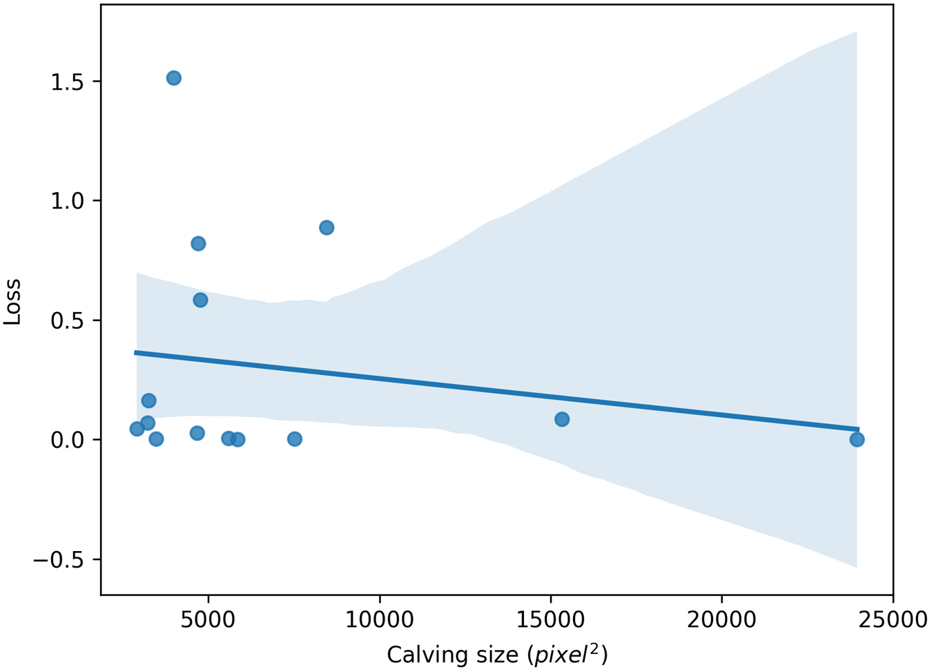
To understand the possible factors influencing the model’s predictions, we investigated the relationship between calving sizes (denoted by the pixel area of the annotation) and the prediction’s loss. It would be expected that larger iceberg calving is more apparent and would be less likely to be misclassified. The calving size and prediction loss were plotted for each of the 14 iceberg calving events in the test dataset, this is shown in Fig. 9. In the graph, we see that in general, higher losses are associated with smaller iceberg calving events. The Pearson correlation coefficient for this data is -0.19, meaning that there was a weak negative correlation but not significant enough to assert a relationship between calving size and loss, indicating that there might be other factors influencing the model’s accuracy. A larger test set would also be required to make any definite conclusions.
Graph plotting the calving size (denoted by the pixel area of the annotation) with the model’s prediction loss. The Pearson correlation coefficient for this graph is -0.19 indicating a weak negative correlation but it is not significant enough to draw conclusions about the model’s prediction ability with respect to the size of the calving. The shaded region is the 95% confidence interval of the regression line.

3.2. Model generalisation to other time periods
3.2.1. Selection of usable images
Further evaluation was performed on the transferability of this method to different time periods using the April 2016 dataset. This dataset was chosen because it features different weather conditions compared to the training and test data. The images were first pre-processed by cropping and rotating to the area of interest with manually chosen parameters specific to this dataset. The images were then manually labelled using CVAT based on their usability classification. Out of the 849 images, 783 images were labelled as usable and 66 as unusable. These steps are in line with the procedure performed on the July 2016 dataset so that a fair comparison could be drawn.
The method achieved an overall accuracy of 96% on the April 2016 dataset, with 97% of usable images and 88% of unusable images correctly classified. These results have comparable accuracy with the results for the July 2016 dataset. This suggests that the model is transferable to datasets for other time periods with minimal changes. Accuracy could possibly be improved by recalibrating the threshold when working with a new dataset by labelling a small number of images to find a more suitable value.
3.2.2. Detection of iceberg calving from image pairs
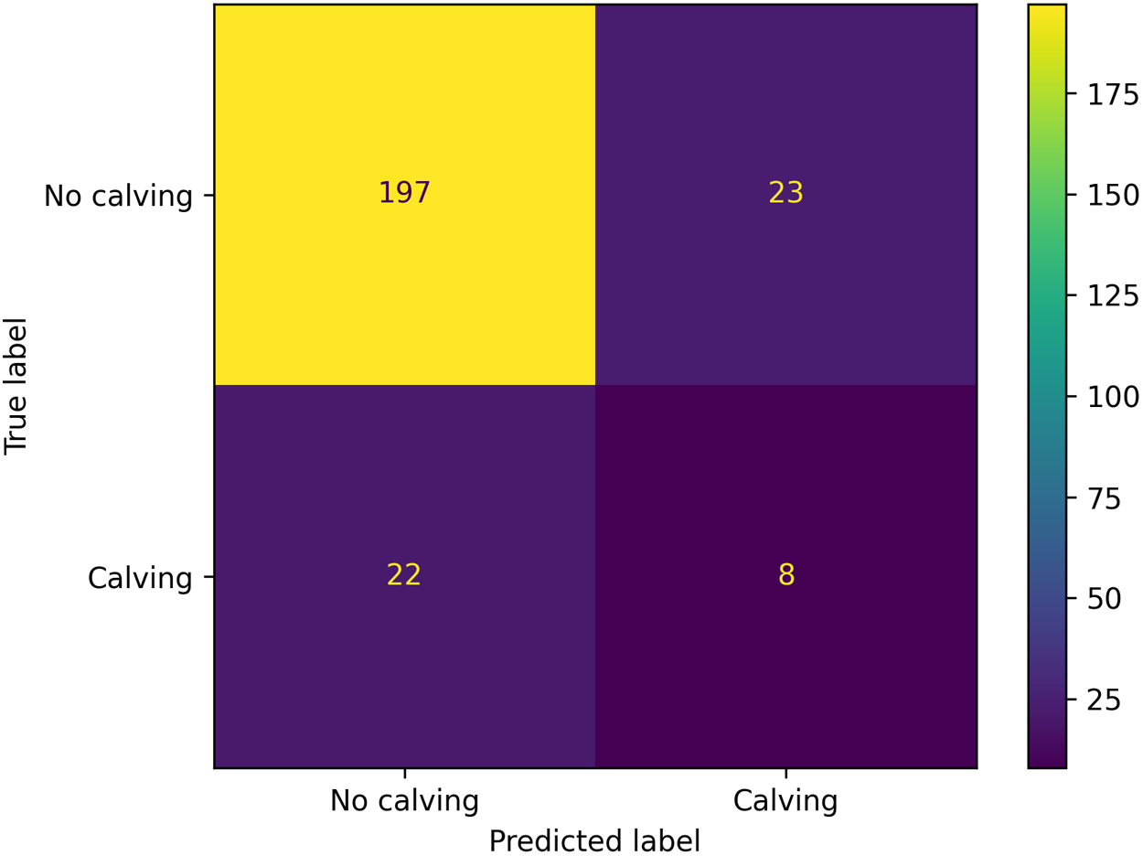
The model’s ability to generalise to other time periods was studied by annotating images from the August 2016 dataset for calving events. We used 250 image pairs, spanning two days, that were manually labelled in the same way as the training and testing data. Data from the month of August was chosen because it has a higher rate of iceberg calving events compared to other months. Then 220 image pairs were labelled to not have iceberg calving events and 30 were labelled to have calving events.
The model achieved an overall accuracy rate of 82% on the unseen data with 90% of non-calving and 27% of calving events being correctly classified. Although a high accuracy was achieved on non-calving, the results indicated that the trained model was not readily transferable to detect calving events in other time periods with an  $F_1$ score of 0.26 (see Fig. 10).
Confusion matrix for model predictions on the unseen August 2016 dataset. An overall accuracy rate of 82% was achieved with 90% of non-calving and 27% of calving events being correctly classified.

The most likely cause of this was that, during training, we used images from the same time period, allowing the neural network to learn features specific to the training data, thereby creating a bias towards it. Training with images from a variety of months could help eliminate this bias and improve the model’s overall accuracy. A gap of 22 days exists between the training and unseen data, which is significant enough that iceberg calving may have altered the appearance of the glacier front, making it less recognisable to the model.
3.3. Analysis of failure cases - methods constraints
3.3.1. Selection of usable images - limitations
In this manuscript, we provided evidence that counting the number of SIFT keypoints for an image is a good way to decide the image’s usability for detection of calving events. The method was shown to perform well on both training and testing data and demonstrated the ability to generalise to other time periods without any modifications, indicating a high degree of suitability for performing the task.
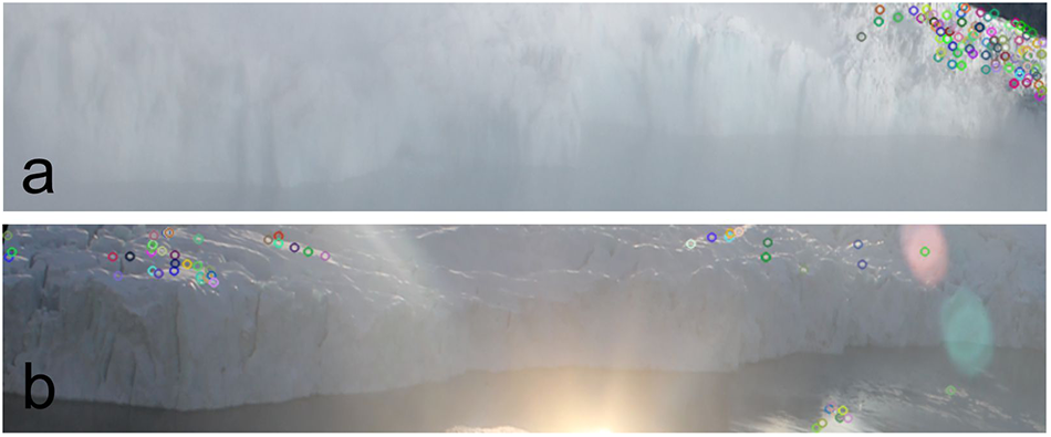
The limitation of this method is that it only counts the number of SIFT key-points in the images without regard for their spatial locations. This can cause images that are partially occluded to still be classified as usable as long as there is a good view for the rest of the glacier (see Fig. 11). Direct comparison of partially occluded images is difficult so the method could be improved to account for this limitation.
Detected SIFT keypoints for unusable images that were wrongly classified as usable, (a) 138 keypoints being detected in a small region but fog covers the rest of the image, (b) sun glare obscuring the centre of the image but the rest of the image retains enough visibility to detect 61 keypoints.

Given the relatively small dataset, it was possible to perform individual analysis on the incorrectly classified test data to understand reasons for the failure and model limitations. Figure 10(a) shows a training example with 138 key-points that was incorrectly classified by our method as usable since the number of key-points was above the threshold of 50. Upon inspection, we see that fog covers the majority of the image but a small section remains clearly visible and key-points can still be detected in that region.
A similar analysis was performed on the April 2016 dataset and it was found that a large number of the misclassified images were affected by sun glare obscuring parts of the glacier front; however, the glare was not spread across the entire image, allowing key-points to still be detected. Figure 10(b) shows one such example where 61 key-points were detected. With a large section of the glacier not clearly visible, we would not be able to properly detect calving events hence why these images were labelled as unusable. This highlights a limitation in our model where only the global count of key-points is considered, whereas the locality of the key-points is not considered.
Our evaluation of the model only included time periods during which the sun remained above the horizon throughout the day and night, ensuring sufficient illumination even under harsh weather conditions. Further analysis could assess the suitability of the developed methods for periods when the sun sets at night, as many images from these months would likely be too dark to detect calving events and would therefore need to be excluded. The results indicate that the model performed well, achieving high accuracy and generalising effectively to other time periods. Nonetheless, the method could be further improved through minor refinements, such as ensuring that key points are distributed across the entire image rather than clustered within a small region. Additionally, implementing dynamic, data-driven threshold selection methods based on statistical analysis could enhance accuracy and reduce the need for manual tuning.
3.3.2. Detection of iceberg calving event from image pairs
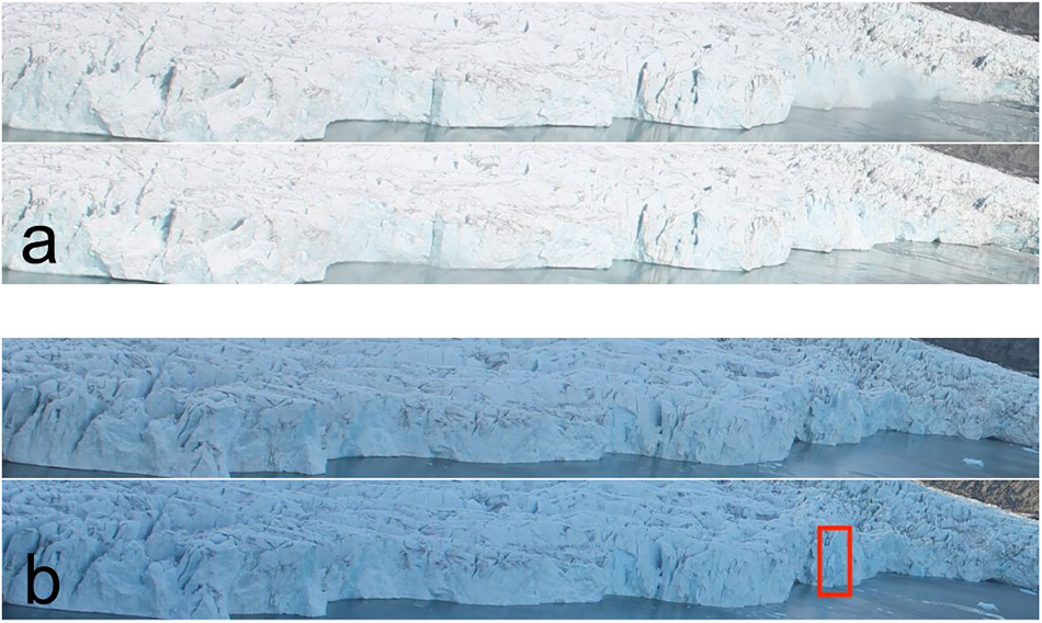
The most common observation for incorrect classification of non-calving events was significant changes in the environment between images. Changes in illumination angles and intensities caused some details to become less visible as they were obscured by shadows and other details would appear more visible. Figure 12 shows a pair of images where no calving occurred but was classified as a calving. Precipitation on the lens caused a distortion in the first image, which disappeared in the subsequent image. The change in the perception of the glacier front was significant enough to be categorised as a calving, when in fact it was not.
Analysis of incorrectly classified image pairs, (a) non-calving event incorrectly classified as a calving due to precipitation on the lens causing a distortion in the first image, which disappeared in the subsequent image. This resulted in a significant change in the appearance of the glacier front which was misattributed to a calving event, (b) calving event incorrectly classified as a non-calving due to the environment being dimly lit and the calving size is relatively small, leading to only a small change on the glacier front, making it harder for the model to detect the change.

Failures to correctly detect the occurrence of a calving accounted for 27% of failure cases and it was observed that most of these failures were characterised by small calving event or insufficient light, meaning that the features were likely not defined enough to be represented in the feature maps. Figure 12 shows one such example where the environment is dimly lit and the calving volume is relatively small. The calving did not create significant change in appearance between the images, making it harder to detect.
It is not surprising that most failures occurred due to non-calving events being attributed to calving, owing to dramatic differences between images caused by environmental factors. This was a challenge that was also noted during manual labelling where the occurrence of calving event was not imminently clear.
3.3.3. Methods limitation and future works
The method presented in this paper has proven to be successful when analysing the Hansbreen dataset. However, similar to other emerging methods, it has its limitations. In the described pipeline, we presented a method for removing unusable images that suffer from extreme weather conditions or other factors obscuring the area of interest. However, we did not address colour unification, which could become problematic when analysing a larger dataset, particularly due to the extreme lighting conditions often observed in spring and autumn. This can be addressed by some of the already existing methods (Vanrell and others, Reference Vanrell, Lumbreras, Pujol, Baldrich, Llados and Villanueva2001; Riabchenko and others, Reference Riabchenko, Lankinen, Buch, Kämäräinen and Krüger2013). Another significant limitation when attempting to automatically process large datasets is the lack of correction for image rotation. The Hansbreen dataset is known to exhibit some rotation between sets of images. This is due to the way the data are acquired from the camera, and occasionally because animals use the cameras as scratching posts. While there are existing methods that could address this issue, we have so far been unsuccessful in identifying a single, definitive solution suitable for this particular dataset. Also, the method in its current iteration does not calculate the volume or size of ice lost during each calving event. This is because, in the initial stages of the project, our focus was primarily on identifying the areas where calving occurred and tracking their movement over time. However, as the project has progressed, we recognise that estimating ice loss volume is an important objective. This aspect will need to be addressed in the future using methods similar to those applied in previous studies focused on volumetric analysis (Adinugroho and others, Reference Adinugroho, Vallot, Westrin and Strand2015; Vallot and others, Reference Vallot2019).
Future work will be divided into two stages. The first stage will focus on applying this and other similar methods to detect calving events across different datasets, with the goal of creating a suitable benchmark for future glacier calving detection studies. This will also include a human-in-the-loop approach to assess the accuracy of manually labelled training datasets. The second stage will concentrate on completing the processing of the entire Hansbreen dataset in order to enrich the existing data with pre-processed imagery for use in further research.
3.4. Conclusions
We have shown that the chosen neural network architecture (SNN architecture) and training method to be suitable for approaching the problem of detecting calving events. A reasonable accuracy rate is achieved on the test data with a low rate of false negatives, so calving events are rarely misclassified. A high number of false positives occurs due to the challenge involved in detecting the small changes of iceberg calving when the environment is variable. The accuracy of the presented model is good enough to be used as a first-pass tool to significantly reduce the number of images that would need to be manually sorted. Considering our test data, it reduced the dataset from 130 pairs to 19, equating to a reduction of 85% of the dataset.
The model required the removal of about 10% of images to detect calving events that means that it still detects the events on images that were not taken in perfect conditions. Other methods, for example Vallot and others (Reference Vallot2019), require up to 45% of images were discarded due to weather effects however they used a different data set thus this is not a direct comparison. However, this is still a high ratio of removed images to usable images. This is why the proposed model could not be trained on a generalised dataset, resulting in reduced performance on unseen data from a different month. Additional data would also help to improve overall accuracy as neural networks have been shown to benefit greatly from large training datasets (Shorten and Khoshgoftaar, Reference Shorten and Khoshgoftaar2019).
The chosen method is shown to be a good basis for a model to detect calving events from time-lapse imagery, with the use of transfer learning being a good approach to reducing training times. The method has the potential to increase its accuracy by exploring variations to the model such as changing the number of convolutional layers used before the linear layers or exploring other convolutional networks other than VGG.
Data availability
The code used in this paper is available online (https://github.com/waps101/calvingdetection/). All data is available online (https://dataportal.igf.edu.pl/organization/polar-and-marine-research).
Acknowledgements
This research has been supported by the National Science Centre, Poland (grant 2021/43/D/ST10/00616) and the Ministry of Science and Higher Education of Poland (subsidy for the Institute of Geophysics, Polish Academy of Sciences). We would like to thank Dr. Mateusz Moskalik for establishing the photographic monitoring of Hansbreen. We also express our gratitude to the crew of the Polish Polar Station Hornsund for the logistical support during data collection and to the reviewers and editors for publishing this paper.




 Open access

