


Impact Statement
This article provides a framework to reduce the global warming potential of civil structures such as bridges, dams, or buildings while satisfying constraints relating to structural efficiency. The framework combines mixture design and structural simulation in a joint workflow to enable optimization. Advanced optimization algorithm with appropriate extensions and heuristics are employed to account for stochasticity of workflow, nonlinear constraints, and lack of derivatives of the workflow. Some relations in the workflow are not known a priori in the literature. These are learned by employing advanced probabilistic machine learning algorithms trained using the fusion of noisy data and physical models. Various forms of uncertainty arising due to noise in the data or incompleteness of data are systematically incorporated into the framework. The big idea here is to create structures with a smaller environmental footprint without compromising their strength while being cost-efficient for the manufacturer. The proposed holistic approach is demonstrated on a specific design problem, but should serve as a template that can be readily adapted to other design problems.
1. Introduction
Precast concrete elements play a critical role in achieving efficient, low-cost, and sustainable structures. The controlled manufacturing environment allows for higher quality products and enables the mass production of such elements. In the standard design approach, engineers or architects select the geometry of a structure, estimate the loads, choose mechanical properties, and design the element accordingly. If the results are unsatisfactory, the required mechanical properties are iteratively adjusted, aiming to improve the design. This approach is adequate when the choice of mixtures is limited, and the expected concrete properties are well known. There are various published methods to automate this process and optimize the beam design at this level. Computer-aided beam design optimization dates back at least 50 years (e.g., Haung and Kirmser, Reference Haung and Kirmser1967).
Generally, the objective is to reduce costs, with the design variables being the beam geometry, the amount and location of the reinforcement, and the compressive strength of the concrete (Chakrabarty, Reference Chakrabarty1992; Coello et al., Reference Coello, Hernández and Farrera1997; Pierott et al., Reference Pierott, Hammad, Haddad, Garcia and Falcón2021; Shobeiri et al., Reference Shobeiri, Bennett, Xie and Visintin2023). Most publications focus on analytical functions based on well-known, empirical rules of thumb. In recent years, the use of alternative binders in the concrete mix design has increased, mainly to reduce the environmental impact and cost of concrete but also to improve and modify specific properties. This is a challenge as the concrete mix is no longer a constant and is itself subject to an optimization. Known heuristics might no longer apply to the new materials, and old design approaches might fail to produce optimal results. In addition, it is not desirable to choose from a predetermined set of possible mixes, as this would lead to either an overwhelming number of required experiments or a limiting subset of the possible design space.
In the existing literature on the optimization of the concrete mix design (Lisienkova et al., Reference Lisienkova, Shindina, Orlova and Komarova2021; Kondapally et al., Reference Kondapally, Chepuri, Elluri and Reddy2022; Forsdyke et al., Reference Forsdyke, Zviazhynski, Lees and Conduit2023), the objective is either to improve mechanical properties like durability within constraints or to minimize, for example, the amount of concrete while keeping other properties above a threshold. A first step to address these limitations is incorporating the compressive strength during optimization in the beam design phase. Higher compressive strength usually correlates with a larger amount of cement and, therefore, higher cost as well as a higher global warming potential (GWP). This approach has shown promising results in achieving improved structural efficiency while considering environmental impact (dos Santos et al., Reference dos Santos, Alves and Kripka2023). To be able to find a part specific optimum, individual data of the manufacturer and specific mix options must be integrated. Therefore, there is still a need for a comprehensive optimization procedure that can seamlessly integrate concrete mix design and structural simulations, ensuring structurally sound and buildable elements with minimized environmental impact for part specific data.
When designing elements subjected to various requirements, both on the material and structural levels, including workability of the fresh concrete, durability of the structure, maximum acceptable temperature, minimal cost, and GWP, the optimal solution is not apparent and will change depending on each individual project. In this article, we present a holistic optimization procedure that combines physics-based models and experimental data in order to enable the optimization of the concrete mix design in the presence of uncertainty, with an objective to minimize the GWP. In particular, we employ structural simulations as constraints to ensure structural integrity, limit the maximum temperature, and ensure an adequate time of demolding.
By integrating the concrete mixture optimization and structural design processes, engineers can tailor the concrete properties to meet the specific requirements of the customer and manufacturer. This approach opens up possibilities for performance prediction and optimization for new mixtures that fall outside the standard range of existing ones. To the best of our knowledge, there are no published works that combine the material and structural levels in one flexible optimization framework. In addition to changing the order of the design steps, the proposed framework allows to directly integrate experimental data and propagate the identified uncertainties. This allows a straightforward integration of new data and quantification of uncertainties regarding the predictions. The proposed framework consists of three main parts. The first part introduces an automated and reproducible probabilistic machine learning-based parameter identification method to calibrate the models by using experimental data. The second part focuses on a black-box optimization method for non-differentiable functions, including constraints. The third part presents a flexible workflow combining the models and functions required for the respective problem.
To carry out black-box optimization, we advocate the use of Variational Optimization (Staines and Barber, Reference Staines and Barber2013; Bird et al., Reference Bird, Kunze and Barber2018), which uses stochastic gradient estimators for black-box functions. We utilize this with appropriate enhancements in order to account for the stochastic, nonlinear constraints. Our choice is motivated by three challenges present in the workflow describing the physical process. First, we are limited by the availability of only black-box evaluations of the physical workflow. In many real-world cases involving physics-based solvers/simulators in the optimization process, one resorts to gradient-free optimization (Moré and Wild, Reference Moré and Wild2009; Snoek et al., Reference Snoek, Larochelle and Adams2012). However, the gradient-free methods perform poorly on high-dimensional parametric spaces (Moré and Wild, Reference Moré and Wild2009). Also, it requires more functional evaluations to reach the optimum as compared to gradient-based methods. Recently, stochastic gradient estimators (Mohamed et al., Reference Mohamed, Rosca, Figurnov and Mnih2020) have been used to estimate gradients of black-box functions and, hence, perform gradient-based optimization (Ruiz et al., Reference Ruiz, Schulter and Chandraker2018; Louppe et al., Reference Louppe, Hermans and Cranmer2019; Shirobokov et al., Reference Shirobokov, Belavin, Kagan, Ustyuzhanin and Baydin2020). However, they do not account for the constraints. Second, the presence of nonlinear constraints makes the optimization challenging. Popular gradient-free methods like constrained Bayesian optimization (cBO) (Gardner et al., Reference Gardner, Kusner, Xu, Weinberger and Cunningham2014) and COBYLA (Powell, Reference Powell1994) pose significant challenges when (non)linear constraints are involved (Audet and Kokkolaras, Reference Audet and Kokkolaras2016; Menhorn et al., Reference Menhorn, Augustin, Bungartz and Marzouk2017; Agrawal et al., Reference Agrawal, Ravi, Koutsourelakis and Bungartz2023). The third challenge is the stochasticity of the workflow, discussed in the following paragraph.
The physical workflow comprising physics-based models to link design variables with the objective and constraints poses an information flow-related challenge. Some links leading to the objective/constraints are not known a priori in the literature, thus hindering the optimization process. We propose a method to learn these missing links, parameterized by an appropriate neural network, with the help of (noisy) experimental data and physical models. The unavoidable noise in the data introduces aleatoric uncertainty, or its incompleteness introduces epistemic uncertainty. To account for the presence of these uncertainties, we advocate the links to be probabilistic. The learned probabilistic links tackle the information bottleneck; however, it introduces random parameters in the physical workflow, thus necessitating optimization under uncertainty (OUU) (Acar et al., Reference Acar, Bayrak, Jung, Lee, Ramu and Ravichandran2021; Martins and Ning, Reference Martins and Ning2021; Qiu et al., Reference Qiu, Wu, Elishakoff and Liu2021). Deterministic inputs can lead to a poor-performing design, which OUU tries to tackle by producing a robust and reliable design that is less sensitive to inherent variability. This paradigm of fusing data and physical models to train machine-learning models has been extensively used across engineering and physics in recent years (Koutsourelakis et al., Reference Koutsourelakis, Zabaras and Girolami2016; Fleming, Reference Fleming2018; Baker et al., Reference Baker, Alexander, Bremer, Hagberg, Kevrekidis, Najm, Parashar, Patra, Sethian, Wild and Willcox2019; Karniadakis et al., Reference Karniadakis, Kevrekidis, Lu, Perdikaris, Wang and Yang2021; Karpatne et al., Reference Karpatne, Kannan and Kumar2022; Lucor et al., Reference Lucor, Agrawal and Sergent2022; Agrawal and Koutsourelakis, Reference Agrawal and Koutsourelakis2023; Forsdyke et al., Reference Forsdyke, Zviazhynski, Lees and Conduit2023), colloquially referred to as scientific machine learning (SciML). In contrast to traditional machine learning areas where big data are generally available, engineering and physical applications generally suffer from a lack of data, further complicated by experimental noise. SciML has shown promise in addressing this lack of data. We summarize our key contributions below:
-
• We present an inverse design approach for the precast concrete industry to promote sustainable construction practices.
-
• To achieve the desired goals, we propose an algorithmic framework with two main components. (a) an optimization algorithm that accounts for the presence of various uncertainties, nonlinear constraints, and lack of derivatives and (b) a probabilistic machine learning algorithm that learns the missing relations to enable the optimization, by combining noisy, experimental data with physical models. The algorithmic framework is transferable to several other material, structural, and mechanical design problems.
-
• To assist the optimization procedure, we propose an automated workflow that combines concrete mixture design and structural simulation.
-
• We demonstrate the effectiveness of the algorithmic framework and the workflow, on a precast concrete beam element. We learn the missing probabilistic link between the mixture design variables and finite element (FE) model parameters describing the concrete hydration and homogenization procedure. Subsequently, we optimize mixture design and beam geometry in the presence of uncertainties, with the goal of reducing the GWP while employing structural simulations as constraints to ensure safe and reliable design.
The structure of the rest of this article is as follows. Section 2.1 describes the proposed design approach, and Section 2.2 describes the physical material models and the applied assumptions. Section 2.3 presents the details of the experimental data. Section 2.4 provides an overview of the aforementioned probabilistic links and the optimization procedure. Section 2.5 talks about the methodology employed to learn the probabilistic links based on the experimental data and the physical models. Then Section 2.6 describe the details of the proposed black-box optimization algorithm. In Section 3, we showcase and discuss the results of the numerical experiments combining all the parts, the experimental data, the physical models, the identification of the probabilistic links, and the optimization framework. Finally, in Section 4, we summarize our findings and discuss possible extensions.
1.1. Demonstration problem
In this work, a well-known example of a simply supported, reinforced, rectangular beam has been chosen. The design problem was originally published in Everard and Tanner (Reference Everard and Tanner1966) and illustrated in Figure 1.
Geometry of the design problem of a bending beam with a constant distributed load (dead load and live load with safety factors of 1.35 and 1.5) and a rectangular cross section. The design variable, beam height is denoted by $ h $
.
$ h $
.

It has been used to showcase different optimization schemes (e.g., Chakrabarty, Reference Chakrabarty1992; Coello et al., Reference Coello, Hernández and Farrera1997; Pierott et al., Reference Pierott, Hammad, Haddad, Garcia and Falcón2021). As opposed to the literature where the optimization is often related to costs, we aim to reduce the overall GWP of the part. This objective is particularly meaningful as the cement industry accounts for approximately 8% of the total anthropogenic GWP (Miller et al., Reference Miller, Horvath and Monteiro2016). Reducing the environmental impact of concrete production becomes crucial in the pursuit of sustainable construction practices. In addition, the reduction of the amount of cement in concrete is also correlated to the reduction of cost, as cement is generally the most expensive component of the concrete mix (Paya-Zaforteza et al., Reference Paya-Zaforteza, Yepes, Hospitaler and González-Vidosa2009). There are three direct ways to reduce the GWP of a given concrete part. First, replace the cement with a substitute with a lower carbon footprint. This usually changes mechanical properties and, in particular, their temporal evolution. Second, increase the amount of aggregates, therefore reducing the cement per volume. This also changes effective properties and needs to be balanced with the workability and the limits due to the applications. Third, decrease the overall volume of concrete by improving the topology of the part. In addition, when analyzing the whole life cycle of a structure, both cost and GWP can be reduced by increasing the durability and, therefore, extending its lifetime. To showcase the proposed method’s capability, two design variables have been chosen; the height of the beam and the ratio of ordinary Portland cement (OPC) to its replacement binder ground granulated blast furnace slag (BFS), a by-product of the iron industry. In addition to the static design according to the standard, the problem is extended to include a key performance indicator (KPI) related to the production process in a prefabrication factory that defines the time after which the removal of the formwork can be performed. To approximate this, the point in time when the beam can bear its own weight has been chosen a criterion. Reducing this time equates to being able to produce more parts with the same formwork.
2. Methods
2.1. Design approaches
The conventional method of designing reinforced concrete structures is depicted in Figure 2. The structural engineer starts by choosing a suitable material (e.g., strength class C40/50) and designs the structure, including the geometry (e.g., the height of a beam) and the reinforcement. In the second step, this design is handed over to the material engineer with the constraint that the material properties assumed by the structural engineer have to be met. This lack of coordination strongly restricts the set of potential solutions since structural design and concrete mix design are strongly coupled; for example, a lower strength can be compensated with a larger beam height.
Classical design approach, where the required minimum material properties are defined by the structural engineer which is then passed to the material engineer.

An alternative design workflow is illustrated in Figure 3, which entails inverting the classical design pipeline. The material composition is the input to the material engineer who predicts the corresponding mechanical properties of the material. This includes KPIs related to the material, for example, viscosity/slump test, or simply the water/cement ratio. In a second step, a structural analysis is performed with the material properties as input. This step outputs the structural KPIs such as the load-bearing capacity, the expected lifetime (for a structure susceptible to fatigue), or the GWP of the complete structure. These two (coupled) modules are used within an optimization procedure to estimate the optimal set of input parameters (both on the material level and on the structural level). One of the KPIs is chosen as the objective function (e.g., GWP) and others as constraints (e.g., load-bearing capacity larger than the load, cement content larger than a threshold, viscosity according to the slump test within a certain interval). Note that in order to use such an inverse-design procedure, the forward modeling workflow needs to be automated and subsequently the information needs to be efficiently back-propagated.
Proposed design approach to cast material and structural design into a forward model that is then integrated into a holistic optimization approach.

This article aims to present the proposed methodological framework as well as illustrate its capabilities in the design of a precast concrete element with the objective of reducing the GWP. The constraints employed are related to the structural performance after 28 days as well as the maximum time of demolding after 10 hours. The design/optimization variables are, on the structural level, the height of the beam, and on the material level, the composition of the binder as a mixture of Portland cement and slag. The complete workflow is illustrated in Figure 4.
Workflow to compute key performance indicators from input parameters.

2.2. Workflow for predicting key performance indicators
The workflow consists of four major steps. In the first step, the cement composition (blended cement and slag) defined in the mix composition is used to predict the mechanical properties of the cement paste. This is done using a data-driven approach as discussed in Section 2.4. In the second step, homogenization is used in order to compute the effective, concrete properties based on cement paste and aggregate data. An analytical function is applied for the homogenization based on the Mori–Tanaka scheme (Mori and Tanaka, Reference Mori and Tanaka1973). The third step involves a multi-physics, FE model with two complex constitutive models—a hydration model, which computes the evolution of the degree of hydration (DOH), considering the local temperature and the heat released during the reaction, and a mechanical model, which simulates the temporal evolution of the mechanical properties assuming that those depend on the DOH. The fourth and last model is based on a design code to estimate the amount of reinforcement and predict the load-bearing capacity after 28 days. Subsequent sections will provide insights into how these models function within the optimization framework.
2.2.1. Homogenized concrete parameters
Experimental data for estimating the compressive strength are obtained from concrete specimens measuring the homogenized response of cement paste and aggregates. The mechanical properties of aggregates are known, whereas the cement paste properties have to be inversely estimated. The calorimetry is directly performed for cement paste.
In order to relate macroscopic mechanical properties to the individual constituents (cement paste and aggregates), an analytical homogenization procedure is used. The homogenized effective concrete properties are the Young modulus $ E $
, the Poisson ratio
$ E $
, the Poisson ratio $ \nu $
, the compressive strength
$ \nu $
, the compressive strength $ {f}_c $
, the density
$ {f}_c $
, the density $ \rho $
, the thermal conductivity
$ \rho $
, the thermal conductivity $ \chi $
, the heat capacity
$ \chi $
, the heat capacity $ C $
, and the total heat release
$ C $
, and the total heat release $ {Q}_{\infty } $
. Depending on the physical meaning, these properties need slightly different methods to estimate the effective concrete properties. The elastic, isotropic properties
$ {Q}_{\infty } $
. Depending on the physical meaning, these properties need slightly different methods to estimate the effective concrete properties. The elastic, isotropic properties $ E $
and
$ E $
and $ \nu $
of the concrete are approximated using the Mori–Tanaka homogenization scheme (Mori and Tanaka, Reference Mori and Tanaka1973). The method assumes spherical inclusions in an infinite matrix and considers the interactions of multiple inclusions. Details are given in Appendix A.1.
$ \nu $
of the concrete are approximated using the Mori–Tanaka homogenization scheme (Mori and Tanaka, Reference Mori and Tanaka1973). The method assumes spherical inclusions in an infinite matrix and considers the interactions of multiple inclusions. Details are given in Appendix A.1.
The estimation of the concrete compressive strength $ {f}_{c,\mathrm{eff}} $
follows the ideas of Nežerka et al. (Reference Nežerka, Hrbek, Prošek, Somr, Tesárek and Fládr2018). The premise is that a failure in the cement paste will cause the concrete to crack. The approach is based on two main assumptions. First, the Mori–Tanaka method is used to estimate the average stress within the matrix material
$ {f}_{c,\mathrm{eff}} $
follows the ideas of Nežerka et al. (Reference Nežerka, Hrbek, Prošek, Somr, Tesárek and Fládr2018). The premise is that a failure in the cement paste will cause the concrete to crack. The approach is based on two main assumptions. First, the Mori–Tanaka method is used to estimate the average stress within the matrix material $ {\sigma}^{(m)} $
. Second, the von Mises failure criterion of the average matrix stress is used to estimate the uniaxial compressive strength (see Appendix A.1.1).
$ {\sigma}^{(m)} $
. Second, the von Mises failure criterion of the average matrix stress is used to estimate the uniaxial compressive strength (see Appendix A.1.1).
Table 1 gives an overview of the material properties of the constituents used in the subsequent sensitivity studies. The effective properties as a function of the aggregate content are plotted in Figure 5. Note that both extremes (0 [pure cement] and 1 [only aggregates]) are purely theoretical.
Properties of the cement paste and aggregates used in subsequent sensitivity studies

Influence of aggregate ratio on effective concrete properties.

For the considered example, the relations are close to linear. This can change when the difference between the matrix and the inclusion properties is more pronounced or more complex micromechanical mechanisms are incorporated, such as air pores or the interfacial transition zone. Though not done in this article, these could be considered within the chosen homogenization scheme by adding additional phases (cf. Nežerka and Zeman, Reference Nežerka and Zeman2012). Homogenization of the thermal conductivity is also based on the Mori–Tanaka method, following the ideas of Stránský et al. (Reference Stránský, Vorel, Zeman and Šejnoha2011) with details given in Appendix A.1.2. The density $ \rho $
, the heat capacity
$ \rho $
, the heat capacity $ C $
, and the total heat release
$ C $
, and the total heat release $ {Q}_{\infty } $
can be directly computed based on their volume average. As an example for the volume-averaged quantities, the heat release is shown in Figure 5 as it exemplifies the expected linear relation of the volume average as well as the zero heat output of a theoretical pure aggregate.
$ {Q}_{\infty } $
can be directly computed based on their volume average. As an example for the volume-averaged quantities, the heat release is shown in Figure 5 as it exemplifies the expected linear relation of the volume average as well as the zero heat output of a theoretical pure aggregate.
2.2.2. Hydration and evolution of mechanical properties
Due to a chemical reaction (hydration) of the binder with water, calcium-silicate hydrates form that lead to a temporal evolution of concrete strength and stiffness. The reaction is exothermal and the kinetics are sensitive to the temperature. The primary model simulates the hydration process and computes the temperature field $ T $
and the DOH
$ T $
and the DOH $ \alpha $
(see Eqs. (B1) and (B2) in Appendix B). The latter characterizes the DOH that condenses the complex chemical reactions into a single scalar variable. The thermal model depends on three material properties: the effective thermal conductivity
$ \alpha $
(see Eqs. (B1) and (B2) in Appendix B). The latter characterizes the DOH that condenses the complex chemical reactions into a single scalar variable. The thermal model depends on three material properties: the effective thermal conductivity $ \lambda $
, the specific heat capacity
$ \lambda $
, the specific heat capacity $ C $
, and the heat release
$ C $
, and the heat release $ \frac{\partial Q}{\partial t} $
. The latter is governed by the hydration model, characterized by six parameters:
$ \frac{\partial Q}{\partial t} $
. The latter is governed by the hydration model, characterized by six parameters: $ {B}_1,{B}_2,\eta, {T}_{\mathrm{ref}},{E}_a $
, and
$ {B}_1,{B}_2,\eta, {T}_{\mathrm{ref}},{E}_a $
, and $ {\alpha}_{\mathrm{max}} $
. The first three
$ {\alpha}_{\mathrm{max}} $
. The first three $ {B}_1,{B}_2 $
, and
$ {B}_1,{B}_2 $
, and $ \eta $
are parameters characterizing the shape of the evolution of the heat release.
$ \eta $
are parameters characterizing the shape of the evolution of the heat release. $ {T}_{\mathrm{ref}} $
is the reference temperature for which the first three parameters are calibrated. (Based on the difference between the actual and the reference temperature, the heat released is scaled.) The sensitivity to the temperature is characterized by the activation energy
$ {T}_{\mathrm{ref}} $
is the reference temperature for which the first three parameters are calibrated. (Based on the difference between the actual and the reference temperature, the heat released is scaled.) The sensitivity to the temperature is characterized by the activation energy $ {E}_a $
.
$ {E}_a $
. $ {\alpha}_{\mathrm{max}} $
is the maximum DOH that can be reached. Following Mills (Reference Mills1966), the maximum DOH is estimated based on the water to binder ratio
$ {\alpha}_{\mathrm{max}} $
is the maximum DOH that can be reached. Following Mills (Reference Mills1966), the maximum DOH is estimated based on the water to binder ratio $ {r}_{\mathrm{wc}} $
, as
$ {r}_{\mathrm{wc}} $
, as $ {\alpha}_{\mathrm{max}}=\frac{1.031\hskip0.1em {r}_{\mathrm{wc}}}{0.194+{r}_{\mathrm{wc}}} $
.
$ {\alpha}_{\mathrm{max}}=\frac{1.031\hskip0.1em {r}_{\mathrm{wc}}}{0.194+{r}_{\mathrm{wc}}} $
.
By assuming the DOH to be the fraction of the currently released heat with respect to its theoretical potential $ {Q}_{\infty } $
, the current DOH is estimated as
$ {Q}_{\infty } $
, the current DOH is estimated as $ \alpha (t)=\frac{Q(t)}{Q_{\infty }} $
. As the potential heat release is also difficult to measure as it takes a long time to fully hydrate and will only do so under perfect conditions, we identify it as an additional parameter in the model parameter estimation. For a detailed model description, see Appendix B. In addition to influencing the reaction speed, the computed temperature is used to verify that the maximum temperature during hydration does not exceed a limit of
$ \alpha (t)=\frac{Q(t)}{Q_{\infty }} $
. As the potential heat release is also difficult to measure as it takes a long time to fully hydrate and will only do so under perfect conditions, we identify it as an additional parameter in the model parameter estimation. For a detailed model description, see Appendix B. In addition to influencing the reaction speed, the computed temperature is used to verify that the maximum temperature during hydration does not exceed a limit of $ {T}_{\mathrm{limit}}=60{}^{\circ}\mathrm{C} $
. Above a certain temperature, the hydration reaction changes (e.g., secondary ettringite formation) and, additionally, volumetric changes in the cooling phase correlate with cracking and reduced mechanical properties. The maximum temperature is implemented as a constraint for the optimization problem (see Eq. (B19)).
$ {T}_{\mathrm{limit}}=60{}^{\circ}\mathrm{C} $
. Above a certain temperature, the hydration reaction changes (e.g., secondary ettringite formation) and, additionally, volumetric changes in the cooling phase correlate with cracking and reduced mechanical properties. The maximum temperature is implemented as a constraint for the optimization problem (see Eq. (B19)).
The evolution of the Young modulus $ E $
of a linear-elastic material model is modeled as a function of the DOH (details in Eq. (B17)). In a similar way, the compressive strength evolution is computed (see Eq. (B15)), which is utilized to determine a failure criterion based on the computed local stresses (Eq. (B20)) related to the time when the formwork can be removed. For a detailed description of the parameter evolution as a function of the DOH, see Appendix B.2. Figure 6 shows the influence of the different parameters. In addition to the formulations given in Carette and Staquet (Reference Carette and Staquet2016) which depend on a theoretical value of parameters for fully hydrated concrete at
$ E $
of a linear-elastic material model is modeled as a function of the DOH (details in Eq. (B17)). In a similar way, the compressive strength evolution is computed (see Eq. (B15)), which is utilized to determine a failure criterion based on the computed local stresses (Eq. (B20)) related to the time when the formwork can be removed. For a detailed description of the parameter evolution as a function of the DOH, see Appendix B.2. Figure 6 shows the influence of the different parameters. In addition to the formulations given in Carette and Staquet (Reference Carette and Staquet2016) which depend on a theoretical value of parameters for fully hydrated concrete at $ \alpha =1 $
, this work reformulates the equations, to depend on the 28 day values
$ \alpha =1 $
, this work reformulates the equations, to depend on the 28 day values $ {E}_{28} $
and
$ {E}_{28} $
and $ {f}_{c28} $
as well as the corresponding
$ {f}_{c28} $
as well as the corresponding $ {\alpha}_{28} $
which is obtained via a simulation. This allows us to directly use the experimental values as input. In Figure 6,
$ {\alpha}_{28} $
which is obtained via a simulation. This allows us to directly use the experimental values as input. In Figure 6, $ {\alpha}_{28} $
is set to
$ {\alpha}_{28} $
is set to $ 0.8 $
.
$ 0.8 $
.
Influence of parameters $ {\alpha}_t,{a}_E $
, and
$ {\alpha}_t,{a}_E $
, and $ {a}_{f_c} $
on the evolution the Young modulus and the compressive strength with respect to the degree of hydration
$ {a}_{f_c} $
on the evolution the Young modulus and the compressive strength with respect to the degree of hydration $ \alpha $
. Parameters:
$ \alpha $
. Parameters: $ {E}_{28}=50\hskip0.22em \mathrm{GPa} $
,
$ {E}_{28}=50\hskip0.22em \mathrm{GPa} $
, $ {a}_E=0.5 $
,
$ {a}_E=0.5 $
, $ {\alpha}_t=0.2 $
,
$ {\alpha}_t=0.2 $
, $ {a}_{f_c}=0.5 $
,
$ {a}_{f_c}=0.5 $
, $ {f}_{c28}=30\hskip0.22em \mathrm{N}/{\mathrm{mm}}^2 $
,
$ {f}_{c28}=30\hskip0.22em \mathrm{N}/{\mathrm{mm}}^2 $
, $ {\alpha}_{28}=0.8 $
.
$ {\alpha}_{28}=0.8 $
.

2.2.3. Beam design according to EC2
The design of the reinforcement and the computation of the load-bearing capacity is performed based on DIN EN 1992-1-1 (2011) according to Eq. (C7) with a detailed explanation in the Appendix C. To ensure that the design is realistic, the continuous cross section is transformed into a discrete number of bars with a diameter chosen from a list. This is visible in Figure 7 by the stepwise increase in cross sections. The admissible results are restricted by two constraints. One is coming from a minimal required compressive strength (Eq. (C8)), visualized as a dashed line. The other, based on the available space to place bars with admissible spacing (Eq. (C13)), visualized as the dotted line. Further details on the computation are given in Appendix C. A sensitivity study for the mutual interaction and the constraints is visualized in Figure 7. The parameters for the sensitivity study are given in Table D1 in Appendix D.
Influence of beam height, concrete compressive strength, and load in the center of the beam on the required steel. The dashed lines represent the minimum compressive strength constraint (Eq. (C8)), and the dotted lines represent the geometrical constraint from the spacing of the bars (Eq. (C13)).

2.2.4. Computation of GWP
The computation of the GWP is performed by multiplying the volume content of each individual material by its specific GWP. The values used in this study are extracted from Braga et al. (Reference Braga, Silvestre and de Brito2017) and listed in Table 2.
Specific global warming potential of the raw materials used in the design

We note that the question of what exactly to include in the GWP computation is largely open. For example, the transport of materials, while non-negligible, is difficult in general to include. Furthermore, there are always local conditions (e.g., the GWP of the energy sources used in the cement production depends on the amount of green energy in that country). In addition, the time span (complete life cycle analysis vs. production) is a point of debate and finally the usage of by-products (slag is currently a by-product of steel manufacturing and thus its GWP is considered to be small). There are currently efforts, both at the national and international levels, to standardize the computation of the GWP or similar quantities. Once these are available, they can be readily integrated into the proposed approach. Such a standardized computation of the GWP can lead either to taxing GWP or to introducing a sustainability limit state, though this is an ongoing discussion in standardization committees.
2.3. Experimental data
This section describes the data used for learning the missing (probabilistic) links (detailed in Section 2.5) between the slag–binder mass ratio $ {r}_{\mathrm{sb}} $
and physical model parameters. The slag–binder mass ratio
$ {r}_{\mathrm{sb}} $
and physical model parameters. The slag–binder mass ratio $ {r}_{\mathrm{sb}} $
is the mass ratio between the amount of BFS and the binder (sum of BFS and OPC). The data are sourced from Gruyaert (Reference Gruyaert2011). In particular, we are concerned about the parameter estimation for the concrete homogenization discussed in Section 2.2.1 and the hydration model in Section 2.2.2.
$ {r}_{\mathrm{sb}} $
is the mass ratio between the amount of BFS and the binder (sum of BFS and OPC). The data are sourced from Gruyaert (Reference Gruyaert2011). In particular, we are concerned about the parameter estimation for the concrete homogenization discussed in Section 2.2.1 and the hydration model in Section 2.2.2.
For concrete homogenization, six different tests for varying ratios $ {r}_{\mathrm{sb}}=\left\{\mathrm{0.0,0.15,0.3,0.5,0.7,0.85}\right\} $
are available for the concrete compressive strength
$ {r}_{\mathrm{sb}}=\left\{\mathrm{0.0,0.15,0.3,0.5,0.7,0.85}\right\} $
are available for the concrete compressive strength $ {f}_c $
after 28 days. For the concrete hydration, we utilize isothermal calorimetry data at
$ {f}_c $
after 28 days. For the concrete hydration, we utilize isothermal calorimetry data at $ 20{}^{\circ}\mathrm{C} $
. We have temporal evolution data of cumulative heat of hydration
$ 20{}^{\circ}\mathrm{C} $
. We have temporal evolution data of cumulative heat of hydration $ \hat{\boldsymbol{Q}} $
for four different values of
$ \hat{\boldsymbol{Q}} $
for four different values of $ {r}_{\mathrm{sb}}=\left\{\mathrm{0.0,0.30,0.50,0.85}\right\} $
. For details on other material parameters and phenomenological values used to obtain the data, the reader is directed to Gruyaert (Reference Gruyaert2011).
$ {r}_{\mathrm{sb}}=\left\{\mathrm{0.0,0.30,0.50,0.85}\right\} $
. For details on other material parameters and phenomenological values used to obtain the data, the reader is directed to Gruyaert (Reference Gruyaert2011).
2.3.1. Young’s modulus E based on fc
The dataset does not encompass information about the Young modulus. Given its significance for the FEM simulation, we resort to a phenomenological approximation derived from ACI Committee 363 (2010). This approximation relies on the compressive strength $ {f}_c $
and the density
$ {f}_c $
and the density $ \rho $
to estimate the Young modulus
$ \rho $
to estimate the Young modulus
 $$ E=3,320\sqrt{f_c}+6,895{\left(\frac{\rho }{2,320}\right)}^{1.5}, $$
with $ \rho $
in kilogram per cubic meter and
$ \rho $
in kilogram per cubic meter and $ {f}_c $
and
$ {f}_c $
and $ E $
in megapascals.
$ E $
in megapascals.
2.4. Model learning and optimization
The workflow illustrated in Figure 4, which builds the link between the parameters relevant to the concrete mix design and the KPIs involving the environmental impact and the structural performance, can be represented in terms of the probabilistic graph (Koller and Friedman, Reference Koller and Friedman2009) shown in Figure 8. As discussed in the Introduction (Section 1), the goal of the present study is to find the value of the design variables $ \boldsymbol{x} $
(concrete mix design and beam geometry) which minimizes the objective
$ \boldsymbol{x} $
(concrete mix design and beam geometry) which minimizes the objective $ \mathcal{O} $
(environmental impact), while satisfying a given set of constraints
$ \mathcal{O} $
(environmental impact), while satisfying a given set of constraints $ {\mathcal{C}}_i $
(beam design criterion, structural performance, etc.). This necessitates forward and backward information flow in the presented graph. The forward information flow is necessary to compute the KPIs for given values of the design variables and the backward information is essentially the sensitivities of the objective and the constraints with respect to the design variables that enable gradient-based optimization. Establishing the information flow poses challenges, which we attempt to tackle with the methods proposed as follows:
$ {\mathcal{C}}_i $
(beam design criterion, structural performance, etc.). This necessitates forward and backward information flow in the presented graph. The forward information flow is necessary to compute the KPIs for given values of the design variables and the backward information is essentially the sensitivities of the objective and the constraints with respect to the design variables that enable gradient-based optimization. Establishing the information flow poses challenges, which we attempt to tackle with the methods proposed as follows:
-
• Data-based model learning: The physics-based models discussed in Sections 2.2.1 and 2.2.2 are used to compute various KPIs (discussed in Figure 8). These depend on some model parameters denoted by $ b $
which are unobserved (latent) in the experiments performed. The model parameters need not only be inferred on the basis of experimental data but also their dependence on the design variables
$ \boldsymbol{x} $
is required in order to be integrated into the optimization framework. In addition, the noise in the data (aleatoric) or the incompleteness of data (epistemic) introduces uncertainty. To this end, we propose learning probabilistic links by employing experimental data as discussed in detail in Section 2.5.
$ b $
which are unobserved (latent) in the experiments performed. The model parameters need not only be inferred on the basis of experimental data but also their dependence on the design variables
$ \boldsymbol{x} $
is required in order to be integrated into the optimization framework. In addition, the noise in the data (aleatoric) or the incompleteness of data (epistemic) introduces uncertainty. To this end, we propose learning probabilistic links by employing experimental data as discussed in detail in Section 2.5. -
• Optimization under uncertainty: The aforementioned uncertainties as well as additional randomness that might be present in the associated links necessitate reformulating the optimization problem (i.e., objectives/constraints) as one of OUU. In turn, this gives rise to new challenges in order to compute the needed derivatives of the KPIs with respect to the design variables which are discussed in Section 2.6.


Stochastic computational graph for the constrained optimization problem for performance-based concrete design: The circles represent stochastic nodes and rectangles deterministic nodes. The design variables are denoted by $ \boldsymbol{x}=\left({x}_1,{x}_2\right) $
. The vector
$ \boldsymbol{x}=\left({x}_1,{x}_2\right) $
. The vector $ b $
represents the unobserved model parameters which are needed in order to link the key performance indicators (KPIs)
$ b $
represents the unobserved model parameters which are needed in order to link the key performance indicators (KPIs) $ \boldsymbol{y}=\left({y}_o,{\left\{{y}_{c_i}\right\}}_{i=1}^I\right) $
with the design variables
$ \boldsymbol{y}=\left({y}_o,{\left\{{y}_{c_i}\right\}}_{i=1}^I\right) $
with the design variables $ \boldsymbol{x} $
. Here,
$ \boldsymbol{x} $
. Here, $ {y}_o $
represents the model output appearing in the optimization objective and
$ {y}_o $
represents the model output appearing in the optimization objective and $ {y}_{c_i} $
represents the model output appearing in the
$ {y}_{c_i} $
represents the model output appearing in the $ i\mathrm{th} $
constraint. The objective function is given by
$ i\mathrm{th} $
constraint. The objective function is given by $ \mathcal{O} $
and the
$ \mathcal{O} $
and the $ i\mathrm{th} $
constraint by
$ i\mathrm{th} $
constraint by $ {\mathcal{C}}_i $
. They are not differentiable with respect to
$ {\mathcal{C}}_i $
. They are not differentiable with respect to $ {x}_1,{x}_2 $
. (Hence,
$ {x}_1,{x}_2 $
. (Hence, $ {x}_1 $
and
$ {x}_1 $
and $ {x}_2 $
are dotted.) The variables
$ {x}_2 $
are dotted.) The variables $ \boldsymbol{\theta} $
are auxiliary and are used in the context of Variational Optimization discussed in Section 2.6.2. Several other deterministic nodes are present between the random variables
$ \boldsymbol{\theta} $
are auxiliary and are used in the context of Variational Optimization discussed in Section 2.6.2. Several other deterministic nodes are present between the random variables $ \boldsymbol{b} $
and the KPIs
$ \boldsymbol{b} $
and the KPIs $ \boldsymbol{y} $
, but they are omitted for brevity. The physical meaning of the variables used is detailed in Table 3.
$ \boldsymbol{y} $
, but they are omitted for brevity. The physical meaning of the variables used is detailed in Table 3.

2.5. Probabilistic links based on data and physical models
This section deals with learning a (probabilistic) model linking the design variables $ \boldsymbol{x} $
and the input parameters of the physics-based models, that is, concrete hydration and concrete homogenization. A graphical representation is contained in Figure 9. Therein,
$ \boldsymbol{x} $
and the input parameters of the physics-based models, that is, concrete hydration and concrete homogenization. A graphical representation is contained in Figure 9. Therein, $ {\left\{{\hat{\boldsymbol{x}}}^{(i)},{\hat{\boldsymbol{z}}}^{(i)}\right\}}_{i=1}^N $
denote the observed data pairs and
$ {\left\{{\hat{\boldsymbol{x}}}^{(i)},{\hat{\boldsymbol{z}}}^{(i)}\right\}}_{i=1}^N $
denote the observed data pairs and $ \boldsymbol{b} $
denotes a vector of unknown and unobserved parameters of the physics-based models and
$ \boldsymbol{b} $
denotes a vector of unknown and unobserved parameters of the physics-based models and $ \boldsymbol{z}\left(\boldsymbol{b}\right) $
the model outputs. The latter relate to an experimental observation
$ \boldsymbol{z}\left(\boldsymbol{b}\right) $
the model outputs. The latter relate to an experimental observation $ {\hat{\boldsymbol{z}}}^{(i)} $
as
$ {\hat{\boldsymbol{z}}}^{(i)} $
as $ {\hat{\boldsymbol{z}}}^{(i)}=\boldsymbol{z}\left({\boldsymbol{b}}^{(i)}\right)+\mathrm{noise} $
, which gives rise to a likelihood
$ {\hat{\boldsymbol{z}}}^{(i)}=\boldsymbol{z}\left({\boldsymbol{b}}^{(i)}\right)+\mathrm{noise} $
, which gives rise to a likelihood $ p\left({\hat{\boldsymbol{z}}}^{(i)}|\boldsymbol{z}\left({\boldsymbol{b}}^{(i)}\right)\right) $
. We further postulate a probabilistic relation between
$ p\left({\hat{\boldsymbol{z}}}^{(i)}|\boldsymbol{z}\left({\boldsymbol{b}}^{(i)}\right)\right) $
. We further postulate a probabilistic relation between $ \hat{\boldsymbol{x}} $
and
$ \hat{\boldsymbol{x}} $
and $ \boldsymbol{b} $
that is expressed by the conditional
$ \boldsymbol{b} $
that is expressed by the conditional $ p\left(\boldsymbol{b}|\boldsymbol{x};\varphi \right) $
, which depends on unknown parameters
$ p\left(\boldsymbol{b}|\boldsymbol{x};\varphi \right) $
, which depends on unknown parameters $ \boldsymbol{\varphi} $
. The physical meaning of the aforementioned variables and model links, as well as of the relevant data, is presented in Table 4. The elements introduced above suggest a Bayesian formulation that can quantify inferential uncertainties in the unknown parameters and propagate it in the model predictions (Koutsourelakis et al., Reference Koutsourelakis, Zabaras and Girolami2016), as detailed in the next section.
$ \boldsymbol{\varphi} $
. The physical meaning of the aforementioned variables and model links, as well as of the relevant data, is presented in Table 4. The elements introduced above suggest a Bayesian formulation that can quantify inferential uncertainties in the unknown parameters and propagate it in the model predictions (Koutsourelakis et al., Reference Koutsourelakis, Zabaras and Girolami2016), as detailed in the next section.
Probabilistic graph for the data and physical model-based model learning. The shaded nodes are the observed and unshaded are the unobserved (latent) nodes.

2.5.1. Expectation–maximization
Given $ N $
data pairs
$ N $
data pairs $ {\mathcal{D}}_N={\left\{{\hat{\boldsymbol{x}}}^{(i)},{\hat{\boldsymbol{z}}}^{(i)}\right\}}_{i=1}^N $
consisting of different concrete mixes and corresponding outputs, we would like to infer the corresponding
$ {\mathcal{D}}_N={\left\{{\hat{\boldsymbol{x}}}^{(i)},{\hat{\boldsymbol{z}}}^{(i)}\right\}}_{i=1}^N $
consisting of different concrete mixes and corresponding outputs, we would like to infer the corresponding $ {\boldsymbol{b}}^{(i)} $
, but more importantly the relation between
$ {\boldsymbol{b}}^{(i)} $
, but more importantly the relation between $ \boldsymbol{x} $
and
$ \boldsymbol{x} $
and $ \boldsymbol{b} $
which would be of relevance for downstream, optimization tasks discussed in Section 2.6.
$ \boldsymbol{b} $
which would be of relevance for downstream, optimization tasks discussed in Section 2.6.
We postulate a probabilistic relation between $ \boldsymbol{x} $
and
$ \boldsymbol{x} $
and $ \boldsymbol{b} $
in the form of a conditional density
$ \boldsymbol{b} $
in the form of a conditional density $ p\left(\boldsymbol{b}|\boldsymbol{x};\boldsymbol{\varphi} \right) $
parametrized by
$ p\left(\boldsymbol{b}|\boldsymbol{x};\boldsymbol{\varphi} \right) $
parametrized by $ \boldsymbol{\varphi} $
. For example,
$ \boldsymbol{\varphi} $
. For example,
 $$ p\left(\boldsymbol{b}|\boldsymbol{x};\boldsymbol{\varphi} \right)=\mathcal{N}\left(\boldsymbol{b}|\hskip0.15em {\boldsymbol{f}}_{\varphi}\left(\boldsymbol{x}\right),\hskip0.35em {\boldsymbol{S}}_{\varphi}\left(\boldsymbol{x}\right)\right), $$
where $ {\boldsymbol{f}}_{\varphi}\left(\boldsymbol{x}\right) $
represents a fully connected, feed-forward neural network parametrized by
$ {\boldsymbol{f}}_{\varphi}\left(\boldsymbol{x}\right) $
represents a fully connected, feed-forward neural network parametrized by $ \boldsymbol{w} $
(further details discussed in Section 3) and
$ \boldsymbol{w} $
(further details discussed in Section 3) and $ {\boldsymbol{S}}_{\varphi}\left(\boldsymbol{x}\right)={\boldsymbol{LL}}^T $
denotes the covariance matrix where
$ {\boldsymbol{S}}_{\varphi}\left(\boldsymbol{x}\right)={\boldsymbol{LL}}^T $
denotes the covariance matrix where $ \boldsymbol{L} $
is lower-triangular. Hence, the parameters
$ \boldsymbol{L} $
is lower-triangular. Hence, the parameters $ \boldsymbol{\varphi} $
to be learned correspond to
$ \boldsymbol{\varphi} $
to be learned correspond to $ \boldsymbol{\varphi} =\left\{\boldsymbol{w},\boldsymbol{L}\right\} $
. We assume that the observations
$ \boldsymbol{\varphi} =\left\{\boldsymbol{w},\boldsymbol{L}\right\} $
. We assume that the observations $ {\hat{\boldsymbol{z}}}^{(i)} $
are contaminated with Gaussian noise, which gives rise to the likelihood:
$ {\hat{\boldsymbol{z}}}^{(i)} $
are contaminated with Gaussian noise, which gives rise to the likelihood:
 $$ p\left({\hat{\boldsymbol{z}}}^{(i)}|\boldsymbol{z}\left({\boldsymbol{b}}^{(i)}\right)\right)=\mathcal{N}\left({\hat{\boldsymbol{z}}}^{(i)}|\boldsymbol{z}\left({\boldsymbol{b}}^{(i)}\right),\hskip0.35em ,{\boldsymbol{\Sigma}}_{\mathrm{\ell}}\right). $$
The covariance $ {\boldsymbol{\Sigma}}_{\mathrm{\ell}} $
depends on the data used and is discussed in Section 3.
$ {\boldsymbol{\Sigma}}_{\mathrm{\ell}} $
depends on the data used and is discussed in Section 3.
Given Eqs. (2) and (3), one can observe that $ {\boldsymbol{b}}^{(i)} $
(i.e., the unobserved model inputs for each concrete mix
$ {\boldsymbol{b}}^{(i)} $
(i.e., the unobserved model inputs for each concrete mix $ i $
) and
$ i $
) and $ \boldsymbol{\varphi} $
would need to be inferred simultaneously. In the following, we obtain point estimates
$ \boldsymbol{\varphi} $
would need to be inferred simultaneously. In the following, we obtain point estimates $ {\boldsymbol{\varphi}}^{\ast } $
for
$ {\boldsymbol{\varphi}}^{\ast } $
for $ \boldsymbol{\varphi} $
, by maximizing the marginal log-likelihood
$ \boldsymbol{\varphi} $
, by maximizing the marginal log-likelihood $ p\left({\mathcal{D}}_N|\boldsymbol{\varphi} \right) $
(also known as log-evidence), that is, the probability that the observed data arose from the model postulated. Hence, we get
$ p\left({\mathcal{D}}_N|\boldsymbol{\varphi} \right) $
(also known as log-evidence), that is, the probability that the observed data arose from the model postulated. Hence, we get
 $$ {\boldsymbol{\varphi}}^{\ast }=\arg \underset{\boldsymbol{\varphi}}{\max}\log \hskip0.35em p\left({\mathcal{D}}_N|\boldsymbol{\varphi} \right). $$
As this is analytically intractable, we propose employing variational Bayesian expectation–maximization (VB-EM) (Beal and Ghahramani, Reference Beal and Ghahramani2003) according to which a lower bound $ \mathrm{\mathcal{F}} $
to the log-evidence (called evidence lower bound [ELBO]) is constructed with the help of auxiliary densities
$ \mathrm{\mathcal{F}} $
to the log-evidence (called evidence lower bound [ELBO]) is constructed with the help of auxiliary densities $ {h}_i\left({\boldsymbol{b}}^{(i)}\right) $
on the unobserved variables
$ {h}_i\left({\boldsymbol{b}}^{(i)}\right) $
on the unobserved variables $ {\boldsymbol{b}}^{(i)} $
:
$ {\boldsymbol{b}}^{(i)} $
:
 $$ \log \hskip0.35em p\left({\mathcal{D}}_N|\varphi \right)\ge \underset{=\mathrm{\mathcal{F}}\left({h}_{1:N},\boldsymbol{\varphi} \right)}{\underbrace{\sum \limits_{i=1}^N{\unicode{x1D53C}}_{h_i\left({\boldsymbol{b}}^{(i)}\right)}\left[\log \frac{p\left({\hat{\boldsymbol{z}}}^{(i)}|\boldsymbol{z}\left({\boldsymbol{b}}^{(i)}\right)\right)p\left({\boldsymbol{b}}^{(i)}|{\boldsymbol{x}}^{(i)};\boldsymbol{\varphi} \right)}{h_i\left({\boldsymbol{b}}^{(i)}\right)}\right]}}, $$
where $ {\unicode{x1D53C}}_{h_i\left({\boldsymbol{b}}^{(i)}\right)}\left[\cdot \right] $
denote the expectation with respect to the auxiliary densities
$ {\unicode{x1D53C}}_{h_i\left({\boldsymbol{b}}^{(i)}\right)}\left[\cdot \right] $
denote the expectation with respect to the auxiliary densities $ {h}_i\left({\boldsymbol{b}}^{(i)}\right) $
on the unobserved variables
$ {h}_i\left({\boldsymbol{b}}^{(i)}\right) $
on the unobserved variables $ {\boldsymbol{b}}^{(i)} $
. Eq. (5) suggests the following iterative scheme where one alternates between the steps:
$ {\boldsymbol{b}}^{(i)} $
. Eq. (5) suggests the following iterative scheme where one alternates between the steps:
-
• E-step: Fix
$ \boldsymbol{\varphi} $
and maximize
$ \mathrm{\mathcal{F}} $
with respect to
$ {h}_i\left({\boldsymbol{b}}^{(i)}\right) $
. It can be readily shown (Bishop and Nasrabadi, Reference Bishop and Nasrabadi2006) that optimality is achieved by the conditional posterior, that is,


 $$ {h}_i^{opt}\left({\boldsymbol{b}}^{(i)}\right)=p\left({\boldsymbol{b}}^{(i)}|{\mathcal{D}}_N,\boldsymbol{\varphi} \right)\propto \hskip0.35em p\left({\hat{\boldsymbol{z}}}^{(i)}|{\boldsymbol{b}}^{(i)}\right)p\left({\boldsymbol{b}}^{(i)}|{\boldsymbol{x}}^{(i)},\boldsymbol{\varphi} \right), $$
which makes the inequality in Eq. (5) tight. Since the likelihood is not tractable as it involves a physics-based solver, we have used Markov chain Monte Carlo (MCMC) to sample from the conditional posterior (see Section 3).
-
• M-step: Given
$ {\left\{{h}_i\left({\boldsymbol{b}}^{(i)}\right)\right\}}_{i=1}^N $
, maximize
$ \mathrm{\mathcal{F}} $
with respect to
$ \boldsymbol{\varphi} $
.


 $$ {\boldsymbol{\varphi}}^{n+1}=\arg \underset{\boldsymbol{\varphi}}{\max}\mathrm{\mathcal{F}}\left({h}_{1:N},{\boldsymbol{\varphi}}^n\right). $$
This requires derivatives of $ \mathrm{\mathcal{F}} $
, that is,
$ \mathrm{\mathcal{F}} $
, that is,
 $$ \frac{\mathrm{\partial \mathcal{F}}}{\partial \boldsymbol{\varphi}}=\sum \limits_{i=1}^N{\unicode{x1D53C}}_{h_i}\left[\frac{\partial \log p\left({\boldsymbol{b}}^{(i)}|{\boldsymbol{x}}^{(i)};\boldsymbol{\varphi} \right)}{\partial \boldsymbol{\varphi}}\right]. $$
Given the MCMC samples $ {\left\{{\boldsymbol{b}}_m^{(i)}\right\}}_{m=1}^M $
from the E-step, these can be approximated as
$ {\left\{{\boldsymbol{b}}_m^{(i)}\right\}}_{m=1}^M $
from the E-step, these can be approximated as
 $$ \frac{\mathrm{\partial \mathcal{F}}}{\partial \varphi}\approx \sum \limits_{i=1}^N\frac{1}{M}\sum \limits_{m=1}^M\frac{\partial \log \hskip0.35em p\left({\boldsymbol{b}}_m^{(i)}|{\boldsymbol{x}}^{(i)};\varphi \right)}{\partial \varphi }. $$
Due to the Monte Carlo noise in these estimates, a stochastic gradient ascent algorithm is utilized. In particular, the ADAM optimizer (Kingma and Ba, Reference Kingma and Ba2014) was used from the PyTorch (Paszke et al., Reference Paszke, Gross, Massa, Lerer, Bradbury, Chanan, Killeen, Lin, Gimelshein, Antiga, Desmaison, Kopf, Yang, DeVito, Raison, Tejani, Chilamkurthy, Steiner, Fang, Bai and Chintala2019) library to capitalize on its auto-differentiation capabilities.
The major elements of the method are summarized in Algorithm 1. We note here that training complexity grows linearly with the number of training samples $ N $
due to the densities
$ N $
due to the densities $ {h}_i $
associated with each data point (for-loop of Algorithm 1), but this can be embarrassingly parallelizable.Footnote 1
$ {h}_i $
associated with each data point (for-loop of Algorithm 1), but this can be embarrassingly parallelizable.Footnote 1
Algorithm 1 Data-based model learning.
1: Input: Data $ {\mathcal{D}}_N={\left\{{\hat{\boldsymbol{x}}}^{(i)},{\hat{\boldsymbol{z}}}^{(i)}\right\}}_{i=1}^N $
, model form
$ {\mathcal{D}}_N={\left\{{\hat{\boldsymbol{x}}}^{(i)},{\hat{\boldsymbol{z}}}^{(i)}\right\}}_{i=1}^N $
, model form $ p\left(\boldsymbol{b}|\boldsymbol{x};\boldsymbol{\varphi} \right) $
, likelihood noise
$ p\left(\boldsymbol{b}|\boldsymbol{x};\boldsymbol{\varphi} \right) $
, likelihood noise $ {\boldsymbol{\Sigma}}_l $
,
$ {\boldsymbol{\Sigma}}_l $
, $ \hskip0.5em n=0 $
2: Output: Learned parameter $ {\boldsymbol{\varphi}}^{\ast } $
3: Initialize the parameters $ \boldsymbol{\varphi} $
4: while ELBO not converged do
Expectation Step (E-step):
5: for $ i=1 $
to
$ i=1 $
to $ N $
do
$ N $
do
6: MCMC to get the posterior probability $ p\left({\boldsymbol{b}}^{(i)}|{\mathcal{D}}_N,{\boldsymbol{\varphi}}^n\right) $
using current
$ p\left({\boldsymbol{b}}^{(i)}|{\mathcal{D}}_N,{\boldsymbol{\varphi}}^n\right) $
using current $ {\boldsymbol{\varphi}}^n $
⊳ Eq. (6)
$ {\boldsymbol{\varphi}}^n $
⊳ Eq. (6)
7: end for
Maximization Step (M-step):
8: Monte Carlo gradient estimate ⊳ Eq. (9)
9: $ {\boldsymbol{\varphi}}^{n+1}=\arg {\max}_{\boldsymbol{\varphi}}\;\mathrm{\mathcal{F}}\left({h}_{1:N},{\boldsymbol{\varphi}}^n\right) $
10: $ n\leftarrow n+1 $
11: end while
Model Predictions: The VB-EM based model learning scheme discussed above can be carried out in an offline phase. Once the model is learned, we are interested in the proposed model’s ability to produce probabilistic predictions (online stage) that reflect the various sources of uncertainty discussed previously. For learnt parameters $ {\boldsymbol{\varphi}}^{\ast } $
, the predictive posterior density
$ {\boldsymbol{\varphi}}^{\ast } $
, the predictive posterior density $ {p}_{\mathrm{pred}}\left(\boldsymbol{z}|\mathcal{D},{\boldsymbol{\varphi}}^{\ast}\right) $
on the solution vector
$ {p}_{\mathrm{pred}}\left(\boldsymbol{z}|\mathcal{D},{\boldsymbol{\varphi}}^{\ast}\right) $
on the solution vector $ \boldsymbol{z} $
of a physical model is as follows:
$ \boldsymbol{z} $
of a physical model is as follows:
 $$ {\displaystyle \begin{array}{l}{p}_{\mathrm{pred}}\left(\boldsymbol{z}|\mathcal{D},{\boldsymbol{\varphi}}^{\ast}\right)=\int p\left(\boldsymbol{z},\boldsymbol{b}|\mathcal{D},{\boldsymbol{\varphi}}^{\ast}\right)\mathrm{d}\boldsymbol{b}\\ {}\hskip8.9em =\int p\left(\boldsymbol{z}|\boldsymbol{b}\right)p\left(\boldsymbol{b}|\mathcal{D},{\boldsymbol{\varphi}}^{\ast}\right)\mathrm{d}\boldsymbol{b}\end{array}} $$
 $$ \approx \frac{1}{K}\sum \limits_{k=1}^K\boldsymbol{z}\left({\boldsymbol{b}}^{(k)}\right). $$
The second of the densities is the conditional (Eq. (2)) substituted with the learned $ {\boldsymbol{\varphi}}^{\ast } $
and the first of the densities is simply a Dirac-delta that corresponds to the solution of the physical model, that is,
$ {\boldsymbol{\varphi}}^{\ast } $
and the first of the densities is simply a Dirac-delta that corresponds to the solution of the physical model, that is, $ \boldsymbol{z}\left(\boldsymbol{b}\right) $
. The intractable integral can be approximated by Monte Carlo using
$ \boldsymbol{z}\left(\boldsymbol{b}\right) $
. The intractable integral can be approximated by Monte Carlo using $ K $
samples of
$ K $
samples of $ \boldsymbol{b} $
drawn from
$ \boldsymbol{b} $
drawn from $ p\left(\boldsymbol{b}|\mathcal{D},{\boldsymbol{\varphi}}^{\ast}\right) $
.
$ p\left(\boldsymbol{b}|\mathcal{D},{\boldsymbol{\varphi}}^{\ast}\right) $
.
2.6. Optimization under uncertainty
With the relevant missing links identified as detailed in the previous section, the optimization can be performed on the basis of Figure 8. We seek to optimize the objective function $ \mathcal{O} $
subject to constraints
$ \mathcal{O} $
subject to constraints $ \mathcal{C}=\left({\mathcal{C}}_1,\dots, {\mathcal{C}}_I\right) $
that are dependent on uncertain parameters
$ \mathcal{C}=\left({\mathcal{C}}_1,\dots, {\mathcal{C}}_I\right) $
that are dependent on uncertain parameters $ \boldsymbol{b} $
, which in turn are dependent on the design variables
$ \boldsymbol{b} $
, which in turn are dependent on the design variables $ \boldsymbol{x} $
. In this setting, the general parameter-dependent nonlinear constrained optimization problem can be stated as
$ \boldsymbol{x} $
. In this setting, the general parameter-dependent nonlinear constrained optimization problem can be stated as
 $$ {\displaystyle \begin{array}{l}\underset{\boldsymbol{x}}{\min}\;\mathcal{O}\left({y}_o\left(\boldsymbol{x},\boldsymbol{b}\right)\right),\\ {}\mathrm{s}.\mathrm{t}.\hskip0.35em {\mathcal{C}}_i\left({y}_{c_i}\left(\boldsymbol{x},\boldsymbol{b}\right)\right)\le 0,\hskip0.35em \forall i\in \left\{1,\dots, I\right\},\end{array}} $$
where $ \boldsymbol{x} $
is a
$ \boldsymbol{x} $
is a $ d $
-dimensional vector of design variables and
$ d $
-dimensional vector of design variables and $ \mathbf{b} $
are the model parameter discussed in the previous section. It can be observed that the optimization problem is nontrivial because of three main reasons: (a) the presence of the constraints (Section 2.6.1), (b) the presence of random variables
$ \mathbf{b} $
are the model parameter discussed in the previous section. It can be observed that the optimization problem is nontrivial because of three main reasons: (a) the presence of the constraints (Section 2.6.1), (b) the presence of random variables $ \boldsymbol{b} $
in the objective and the constraint(s) (Section 2.6.1), and (c) non-differentiability of
$ \boldsymbol{b} $
in the objective and the constraint(s) (Section 2.6.1), and (c) non-differentiability of $ {y}_o,{y}_{c_i} $
and therefore of
$ {y}_o,{y}_{c_i} $
and therefore of $ \mathcal{O} $
and
$ \mathcal{O} $
and $ {\mathcal{C}}_i $
.
$ {\mathcal{C}}_i $
.
2.6.1. Handling stochasticity and constraints
Since the solution of Eq. (12) depends on the random variables $ \boldsymbol{b} $
, the objective and constraints are random variables as well and we have to take their random variability into account. We do this by reverting to a robust optimization problem (Ben-Tal and Nemirovski, Reference Ben-Tal and Nemirovski1999; Bertsimas et al., Reference Bertsimas, Brown and Caramanis2011), with expected values denoted by
$ \boldsymbol{b} $
, the objective and constraints are random variables as well and we have to take their random variability into account. We do this by reverting to a robust optimization problem (Ben-Tal and Nemirovski, Reference Ben-Tal and Nemirovski1999; Bertsimas et al., Reference Bertsimas, Brown and Caramanis2011), with expected values denoted by $ \unicode{x1D53C}\left[\cdot \right] $
being the robustness measure to integrate out the uncertainties. In this manner, the optimization problem in Eq. (12) is reformulated as
$ \unicode{x1D53C}\left[\cdot \right] $
being the robustness measure to integrate out the uncertainties. In this manner, the optimization problem in Eq. (12) is reformulated as
 $$ {\displaystyle \begin{array}{l}\underset{\boldsymbol{x}}{\min}\;{\unicode{x1D53C}}_{\boldsymbol{b}}\left[\mathcal{O}\left({y}_o\left(\boldsymbol{x},\boldsymbol{b}\right)\right)\right],\\ {}\mathrm{s}.\mathrm{t}.\hskip0.35em {\unicode{x1D53C}}_{\mathbf{b}}\left[{\mathcal{C}}_i\left({y}_{c_i}\left(\boldsymbol{x},\boldsymbol{b}\right)\right)\right]\le 0,\hskip0.35em \forall i\in \left\{1,\dots, I\right\}.\end{array}} $$
The expected objective value will yield a design that performs best on average, while the reformulated constraints imply feasibility on average.
One can cast this constrained problem to an unconstrained one using penalty-based methods (Nocedal and Wright, Reference Nocedal and Wright1999; Wang and Spall, Reference Wang and Spall2003). In particular, we define an augmented objective function $ \mathrm{\mathcal{L}} $
as follows:
$ \mathrm{\mathcal{L}} $
as follows:
 $$ \mathrm{\mathcal{L}}\left(\boldsymbol{x},\boldsymbol{b},\boldsymbol{\lambda} \right)=\mathcal{O}\left({y}_o\left(\boldsymbol{x},\boldsymbol{b}\right)\right)+\sum \limits_i{\lambda}_i\max \left({\mathcal{C}}_i\left({y}_{c_i}\left(\boldsymbol{x},\boldsymbol{b}\right)\right),0\right), $$
where $ {\lambda}_i>0 $
is the penalty parameter for the
$ {\lambda}_i>0 $
is the penalty parameter for the $ i\mathrm{th} $
constraint. The larger the
$ i\mathrm{th} $
constraint. The larger the $ {\lambda}_i $
’s are, the more strictly the constraints are enforced. Incorporating the augmented objective (Eq. (14)) in the reformulated optimization problem (Eq. (13)), one can arrive at the following penalized objective:
$ {\lambda}_i $
’s are, the more strictly the constraints are enforced. Incorporating the augmented objective (Eq. (14)) in the reformulated optimization problem (Eq. (13)), one can arrive at the following penalized objective:
 $$ {\unicode{x1D53C}}_{\boldsymbol{b}}\left[\mathrm{\mathcal{L}}\left(\boldsymbol{x},\boldsymbol{b},\boldsymbol{\lambda} \right)\right]=\int \mathrm{\mathcal{L}}\left(\boldsymbol{x},\boldsymbol{b},\boldsymbol{\lambda} \right)p\left(\boldsymbol{b}|\boldsymbol{x},\boldsymbol{\varphi} \right)\mathrm{d}\boldsymbol{b}, $$
leading to the following equivalent, unconstrained optimization problem:
 $$ \underset{\boldsymbol{x}}{\min}\;{\unicode{x1D53C}}_{\boldsymbol{b}}\left[\mathrm{\mathcal{L}}\left(\boldsymbol{x},\boldsymbol{b},\boldsymbol{\lambda} \right)\right]. $$
The expectation above is approximated by Monte Carlo which induces noise and necessitates the use of stochastic optimization methods (discussed in detail in the sequel). Furthermore, we propose to alleviate the dependence on the penalty parameters $ \lambda $
by using the sequential unconstrained minimization technique algorithm (Fiacco and McCormick, Reference Fiacco and McCormick1990), which has been shown to work with nonlinear constraints (Liuzzi et al., Reference Liuzzi, Lucidi and Sciandrone2010). The algorithm considers a strictly increasing sequence
$ \lambda $
by using the sequential unconstrained minimization technique algorithm (Fiacco and McCormick, Reference Fiacco and McCormick1990), which has been shown to work with nonlinear constraints (Liuzzi et al., Reference Liuzzi, Lucidi and Sciandrone2010). The algorithm considers a strictly increasing sequence $ \left\{{\boldsymbol{\lambda}}_n\right\} $
with
$ \left\{{\boldsymbol{\lambda}}_n\right\} $
with $ {\boldsymbol{\lambda}}_n\to \infty $
. Fiacco and McCormick (Reference Fiacco and McCormick1990) proved that when
$ {\boldsymbol{\lambda}}_n\to \infty $
. Fiacco and McCormick (Reference Fiacco and McCormick1990) proved that when $ {\boldsymbol{\lambda}}_n\to \infty $
, then the sequence of corresponding minima, say
$ {\boldsymbol{\lambda}}_n\to \infty $
, then the sequence of corresponding minima, say $ \left\{{\boldsymbol{x}}_n^{\ast}\right\} $
, converges to a global minimizer
$ \left\{{\boldsymbol{x}}_n^{\ast}\right\} $
, converges to a global minimizer $ {\boldsymbol{x}}^{\ast } $
of the original constrained problem. This adaptation of the penalty parameters helps to balance the need to satisfy the constraints with the need to make progress toward the optimal solution.
$ {\boldsymbol{x}}^{\ast } $
of the original constrained problem. This adaptation of the penalty parameters helps to balance the need to satisfy the constraints with the need to make progress toward the optimal solution.
2.6.2. Non-differentiable objective and constraints
We note that the approximation of the objective in Eq. (16) with Monte Carlo requires multiple runs of the expensive, forward, physics-based models involved, at each iteration of the optimization algorithm. In order to reduce the number of iterations required, especially when the dimension of the design space is higher, derivatives of the objective would be needed. In cases where the dimension of the design vector $ \boldsymbol{x} $
is high, gradient-based methods are necessary. In turn, the computation of derivatives of
$ \boldsymbol{x} $
is high, gradient-based methods are necessary. In turn, the computation of derivatives of $ \mathrm{\mathcal{L}} $
would necessitate derivatives of the outputs of the forward models with respect to the optimization variables
$ \mathrm{\mathcal{L}} $
would necessitate derivatives of the outputs of the forward models with respect to the optimization variables $ \boldsymbol{x} $
. The latter are, however, unavailable due to the non-differentiability of the forward models. This is a common, restrictive feature of several physics-based simulators which in most cases of engineering practice are implemented in legacy codes that are run as black boxes. This lack of differentiability has been recognized as a significant roadblock by several researchers in recent years (Beaumont et al., Reference Beaumont, Zhang and Balding2002; Marjoram et al., Reference Marjoram, Molitor, Plagnol and Tavaré2003; Louppe et al., Reference Louppe, Hermans and Cranmer2019; Cranmer et al., Reference Cranmer, Brehmer and Louppe2020; Shirobokov et al., Reference Shirobokov, Belavin, Kagan, Ustyuzhanin and Baydin2020; Lucor et al., Reference Lucor, Agrawal and Sergent2022; Oliveira et al., Reference Oliveira, Scalzo, Kohn, Cripps, Hardman, Close, Taghavi and Lemckert2022; Agrawal and Koutsourelakis, Reference Agrawal and Koutsourelakis2023). In this work, we advocate Variational Optimization (Staines and Barber, Reference Staines and Barber2013; Bird et al., Reference Bird, Kunze and Barber2018), which employs a differentiable bound on the non-differentiable objective. In the context of the current problem, we can write
$ \boldsymbol{x} $
. The latter are, however, unavailable due to the non-differentiability of the forward models. This is a common, restrictive feature of several physics-based simulators which in most cases of engineering practice are implemented in legacy codes that are run as black boxes. This lack of differentiability has been recognized as a significant roadblock by several researchers in recent years (Beaumont et al., Reference Beaumont, Zhang and Balding2002; Marjoram et al., Reference Marjoram, Molitor, Plagnol and Tavaré2003; Louppe et al., Reference Louppe, Hermans and Cranmer2019; Cranmer et al., Reference Cranmer, Brehmer and Louppe2020; Shirobokov et al., Reference Shirobokov, Belavin, Kagan, Ustyuzhanin and Baydin2020; Lucor et al., Reference Lucor, Agrawal and Sergent2022; Oliveira et al., Reference Oliveira, Scalzo, Kohn, Cripps, Hardman, Close, Taghavi and Lemckert2022; Agrawal and Koutsourelakis, Reference Agrawal and Koutsourelakis2023). In this work, we advocate Variational Optimization (Staines and Barber, Reference Staines and Barber2013; Bird et al., Reference Bird, Kunze and Barber2018), which employs a differentiable bound on the non-differentiable objective. In the context of the current problem, we can write
 $$ \underset{\boldsymbol{x}}{\min}\int \left(\mathrm{\mathcal{L}}\left(\boldsymbol{x},\boldsymbol{b},\boldsymbol{\lambda} \right)\right)\hskip0.35em p\left(\boldsymbol{b}|\boldsymbol{x},\boldsymbol{\varphi} \right)\mathrm{d}\boldsymbol{b}\le \underset{U\left(\boldsymbol{\theta} \right)}{\underbrace{\int \left(\mathrm{\mathcal{L}}\left(\boldsymbol{x},\boldsymbol{b},\boldsymbol{\lambda} \right)\right)p\left(\boldsymbol{b}|\boldsymbol{x},\boldsymbol{\varphi} \right)q\left(\boldsymbol{x}|\boldsymbol{\theta} \right)\hskip0.35em \mathrm{d}\boldsymbol{b}\hskip0.35em \mathrm{d}\boldsymbol{x}}}, $$
where $ q\left(\boldsymbol{x}|\boldsymbol{\theta} \right) $
is a density over the design variables
$ q\left(\boldsymbol{x}|\boldsymbol{\theta} \right) $
is a density over the design variables $ \boldsymbol{x} $
with parameters
$ \boldsymbol{x} $
with parameters $ \boldsymbol{\theta} $
. If
$ \boldsymbol{\theta} $
. If $ {\boldsymbol{x}}^{\ast } $
yields the minimum of the objective
$ {\boldsymbol{x}}^{\ast } $
yields the minimum of the objective $ {\unicode{x1D53C}}_{\boldsymbol{b}}\left[\mathrm{\mathcal{L}}\right] $
, then this can be achieved with a degenerate
$ {\unicode{x1D53C}}_{\boldsymbol{b}}\left[\mathrm{\mathcal{L}}\right] $
, then this can be achieved with a degenerate $ q $
that collapses to a Dirac-delta, that is, if
$ q $
that collapses to a Dirac-delta, that is, if $ q\left(\boldsymbol{x}|\boldsymbol{\theta} \right)=\delta \left(\boldsymbol{x}-{\boldsymbol{x}}^{\ast}\right) $
. For all other densities
$ q\left(\boldsymbol{x}|\boldsymbol{\theta} \right)=\delta \left(\boldsymbol{x}-{\boldsymbol{x}}^{\ast}\right) $
. For all other densities $ q $
or parameters
$ q $
or parameters $ \boldsymbol{\theta} $
, the inequality above would in general be strict. Hence, instead of minimizing
$ \boldsymbol{\theta} $
, the inequality above would in general be strict. Hence, instead of minimizing $ {\unicode{x1D53C}}_{\boldsymbol{b}}\left[\mathrm{\mathcal{L}}\right] $
with respect to
$ {\unicode{x1D53C}}_{\boldsymbol{b}}\left[\mathrm{\mathcal{L}}\right] $
with respect to $ \boldsymbol{x} $
, we can minimize the upper bound
$ \boldsymbol{x} $
, we can minimize the upper bound $ U $
with respect to
$ U $
with respect to $ \boldsymbol{\theta} $
. Under mild restrictions outlined by Staines and Barber (Reference Staines and Barber2012), the bound
$ \boldsymbol{\theta} $
. Under mild restrictions outlined by Staines and Barber (Reference Staines and Barber2012), the bound $ U\left(\boldsymbol{\theta} \right) $
is differential with respect to
$ U\left(\boldsymbol{\theta} \right) $
is differential with respect to $ \boldsymbol{\theta} $
, and using the log-likelihood trick, its gradient can be rewritten as (Williams, Reference Williams1992)
$ \boldsymbol{\theta} $
, and using the log-likelihood trick, its gradient can be rewritten as (Williams, Reference Williams1992)
 $$ {\displaystyle \begin{array}{c}{\nabla}_{\boldsymbol{\theta}}U\left(\boldsymbol{\theta} \right)={\unicode{x1D53C}}_{\boldsymbol{x},\boldsymbol{b}}\hskip0.35em \left[{\nabla}_{\boldsymbol{\theta}}\log q\left(\boldsymbol{x}|\boldsymbol{\theta} \right)\mathrm{\mathcal{L}}\Big(\boldsymbol{x},\boldsymbol{b},\boldsymbol{\lambda} \Big)\right]\\ {}\approx \frac{1}{S}\sum \limits_{i=1}^S\;\mathrm{\mathcal{L}}\left({\boldsymbol{x}}_i,{\boldsymbol{b}}_i,\boldsymbol{\lambda} \right)\frac{\partial }{\partial \boldsymbol{\theta}}\log q\left({\boldsymbol{x}}_i|\boldsymbol{\theta} \right).\end{array}} $$
Both terms in the integrand can be readily evaluated which opens the door for a Monte Carlo approximation of the aforementioned expression by drawing samples $ {\boldsymbol{x}}_i $
from
$ {\boldsymbol{x}}_i $
from $ q\left(\boldsymbol{x}|\boldsymbol{\theta} \right) $
and subsequently
$ q\left(\boldsymbol{x}|\boldsymbol{\theta} \right) $
and subsequently $ {\boldsymbol{b}}_i $
from
$ {\boldsymbol{b}}_i $
from $ p\left(\boldsymbol{b}|{\boldsymbol{x}}_i,{\varphi}^{\ast}\right) $
.
$ p\left(\boldsymbol{b}|{\boldsymbol{x}}_i,{\varphi}^{\ast}\right) $
.
2.6.3. Implementation considerations and challenges
While the Monte Carlo estimation of the gradient of the new objective $ U\left(\boldsymbol{\theta} \right) $
also requires running the expensive, forward models multiple times, it can be embarrassingly parallelized.
$ U\left(\boldsymbol{\theta} \right) $
also requires running the expensive, forward models multiple times, it can be embarrassingly parallelized.
Obviously, convergence is impeded by the unavoidable Monte Carlo errors in the aforementioned estimates. In order to reduce them, we advocate the use of the baseline estimator proposed in Kool et al. (Reference Kool, van Hoof and Welling2019), which is based on the following expression:
 $$ \frac{\partial U}{\partial \theta}\approx \frac{1}{S-1}\sum \limits_{i=1}^S\frac{\partial }{\partial \boldsymbol{\theta}}\log q\left({\boldsymbol{x}}_i|\boldsymbol{\theta} \right)\left(\mathrm{\mathcal{L}}\left({\boldsymbol{x}}_i,{\boldsymbol{b}}_i,\boldsymbol{\lambda} \right)-\frac{1}{S}\sum \limits_{j=1}^S\mathrm{\mathcal{L}}\Big({\boldsymbol{x}}_j,{\boldsymbol{b}}_j,\boldsymbol{\lambda} \Big)\right). $$
The estimator above is also unbiased as the one in Eq. (18); it does not imply any additional cost beyond the $ S $
samples and in addition exhibits lower variance as shown in Kool et al. (Reference Kool, van Hoof and Welling2019).
$ S $
samples and in addition exhibits lower variance as shown in Kool et al. (Reference Kool, van Hoof and Welling2019).
To efficiently compute the gradient estimators, we make use of the auto-differentiation capabilities of modern machine learning libraries. In the present study, PyTorch (Paszke et al., Reference Paszke, Gross, Massa, Lerer, Bradbury, Chanan, Killeen, Lin, Gimelshein, Antiga, Desmaison, Kopf, Yang, DeVito, Raison, Tejani, Chilamkurthy, Steiner, Fang, Bai and Chintala2019) was utilized. For the stochastic gradient descent, the ADAM optimizer was used (Kingma and Ba, Reference Kingma and Ba2014). In the present study, $ q\left(\boldsymbol{x}|\boldsymbol{\theta} \right) $
was a Gaussian distribution with parameters
$ q\left(\boldsymbol{x}|\boldsymbol{\theta} \right) $
was a Gaussian distribution with parameters $ \boldsymbol{\theta} =\left\{\boldsymbol{\mu}, \boldsymbol{\Sigma} \right\} $
representing mean and diagonal covariance, respectively. We say we have arrived at an optimal
$ \boldsymbol{\theta} =\left\{\boldsymbol{\mu}, \boldsymbol{\Sigma} \right\} $
representing mean and diagonal covariance, respectively. We say we have arrived at an optimal $ {\boldsymbol{x}}^{\ast } $
when the
$ {\boldsymbol{x}}^{\ast } $
when the $ q $
almost degenerates to a Dirac-delta, or colloquially, when the variance of
$ q $
almost degenerates to a Dirac-delta, or colloquially, when the variance of $ q $
has converged and is considerably small. For completeness, the algorithm for the proposed optimization scheme is given in Algorithm 2. A schematic overview of the methods discussed in Sections 2.5 and 2.6 is presented in Figure 10.
$ q $
has converged and is considerably small. For completeness, the algorithm for the proposed optimization scheme is given in Algorithm 2. A schematic overview of the methods discussed in Sections 2.5 and 2.6 is presented in Figure 10.
A schematic of the probabilistic model learning (left block) and the optimization under uncertainty (OUU; right block). The left block illustrates how the information from experimental data and physical models are fused together to learn the missing probabilistic link. This learned probabilistic link subsequently becomes a linchpin in predictive scenarios, particularly in downstream optimization tasks. The right block illustrates querying the learned probabilistic model to complete the missing link and interfacing the workflow describing the design variables, the physical models, and the key performance indicators. Subsequently, this integrated approach facilitates the execution of OUU as per the proposed methodology.

Possible alternatives to the presented optimization scheme could be the popular gradient-free methods (Audet and Kokkolaras, Reference Audet and Kokkolaras2016) like cBO and the extensions (Gardner et al., Reference Gardner, Kusner, Xu, Weinberger and Cunningham2014) with appropriate adjustments to handle stochasticity, genetic algorithms (Banzhaf et al., Reference Banzhaf, Nordin, Keller and Francone1998), COBYLA (Powell, Reference Powell1994), and evolution strategies (Wierstra et al., Reference Wierstra, Schaul, Glasmachers, Sun, Peters and Schmidhuber2014), to name a few. The gradient-free methods are known to perform poorly in high-dimensions (Moré and Wild, Reference Moré and Wild2009). Since we use the approximate gradient information to move in the parametric space in the presented method, higher-dimensional optimization is feasible, as reported in Staines and Barber (Reference Staines and Barber2012) and Bird et al. (Reference Bird, Kunze and Barber2018). The computational cost naturally scales exponentially with the number of design variables $ d $
, as the number of samples
$ d $
, as the number of samples $ S $
per iteration is usually of the order
$ S $
per iteration is usually of the order $ \mathcal{O}(d) $
(Salimans et al., Reference Salimans, Ho, Chen, Sidor and Sutskever2017). Additionally, if a very expensive simulator is involved in the workflow, the core hours needed would naturally increase as generating each sample would become expensive. Fortunately, as the optimization scheme is embarrassingly parallelizable, physical time would be approximately equal to the time needed for one run of simulator times the number of optimization steps.
$ \mathcal{O}(d) $
(Salimans et al., Reference Salimans, Ho, Chen, Sidor and Sutskever2017). Additionally, if a very expensive simulator is involved in the workflow, the core hours needed would naturally increase as generating each sample would become expensive. Fortunately, as the optimization scheme is embarrassingly parallelizable, physical time would be approximately equal to the time needed for one run of simulator times the number of optimization steps.
The presented optimization scheme has the following limitations, which we will attempt to address in the future. (1) Even after applying the baseline trick, one might observe some oscillations in $ \boldsymbol{\theta} $
space near the optima. As suggested in Wierstra et al. (Reference Wierstra, Schaul, Glasmachers, Sun, Peters and Schmidhuber2014), these can potentially be eased by using natural gradients. (2) The proposed method can get trapped in local optima in highly multimodal surfaces. Casting the objective as
$ \boldsymbol{\theta} $
space near the optima. As suggested in Wierstra et al. (Reference Wierstra, Schaul, Glasmachers, Sun, Peters and Schmidhuber2014), these can potentially be eased by using natural gradients. (2) The proposed method can get trapped in local optima in highly multimodal surfaces. Casting the objective as $ U\left(\boldsymbol{\theta} \right) $
can be seen as a Gaussian blurred version of the original objective, the degree of smoothing being contingent upon the choice of initial
$ U\left(\boldsymbol{\theta} \right) $
can be seen as a Gaussian blurred version of the original objective, the degree of smoothing being contingent upon the choice of initial $ \mathtt{\varSigma} $
. This smoothening essentially helps escape the local optima (also one of the strengths of the method). Still, for a highly multimodal surface (e.g., Ackley function), the smoothening might not be enough, leading to an early convergence to local optima. A safe bet would be to choose “large enough”
$ \mathtt{\varSigma} $
. This smoothening essentially helps escape the local optima (also one of the strengths of the method). Still, for a highly multimodal surface (e.g., Ackley function), the smoothening might not be enough, leading to an early convergence to local optima. A safe bet would be to choose “large enough” $ \mathtt{\varSigma} $
, but this, in turn, might add to the computational cost (Wolpert and Macready, Reference Wolpert and Macready1997). (3) The method might struggle for an objective surface with valleys (e.g., Rosenbrock function). If the dimension is not very high, a full
$ \mathtt{\varSigma} $
, but this, in turn, might add to the computational cost (Wolpert and Macready, Reference Wolpert and Macready1997). (3) The method might struggle for an objective surface with valleys (e.g., Rosenbrock function). If the dimension is not very high, a full $ \mathtt{\varSigma} $
matrix instead of the diagonal might help. (4) The applicability of the proposed workflow for multi-objective optimization is not explored in the present work, but since evolutionary strategies are a class of Variational Optimization and evolutionary strategies are known to work with multi-objective optimization problems (e.g., Deb et al., Reference Deb, Pratap, Agarwal and Meyarivan2002), this might be an interesting research direction.
$ \mathtt{\varSigma} $
matrix instead of the diagonal might help. (4) The applicability of the proposed workflow for multi-objective optimization is not explored in the present work, but since evolutionary strategies are a class of Variational Optimization and evolutionary strategies are known to work with multi-objective optimization problems (e.g., Deb et al., Reference Deb, Pratap, Agarwal and Meyarivan2002), this might be an interesting research direction.
Algorithm 2 Black-box stochastic constrained optimization.
1: Input: distribution $ q\left(\boldsymbol{x}|\boldsymbol{\theta} \right) $
for the design variable
$ q\left(\boldsymbol{x}|\boldsymbol{\theta} \right) $
for the design variable $ \boldsymbol{x} $
,
$ \boldsymbol{x} $
, $ n=0 $
, learning rate
$ n=0 $
, learning rate $ \eta $
2: $ {\boldsymbol{\theta}}_0^0,{\boldsymbol{\lambda}}_1\leftarrow $
choose starting point
$ {\boldsymbol{\theta}}_0^0,{\boldsymbol{\lambda}}_1\leftarrow $
choose starting point
3: for $ k=1,2,\dots $
do
$ k=1,2,\dots $
do
4: while $ {\boldsymbol{\theta}}_k $
not converged do
$ {\boldsymbol{\theta}}_k $
not converged do
5: Sample design variables and model parameters $ {\boldsymbol{x}}_i\sim q\left(\boldsymbol{x}|{\boldsymbol{\theta}}_k^n\right),\hskip1em {\boldsymbol{b}}_i\sim p\left(\boldsymbol{b}|{\boldsymbol{x}}_i,\boldsymbol{\varphi} \right) $
6: Farm the workflow with physics-based solvers for the samples in different machines and compute updated objective $ \mathrm{\mathcal{L}}\left({\boldsymbol{x}}_i,{\boldsymbol{b}}_i,{\boldsymbol{\lambda}}_k\right) $
for each of them ⊳ Eq. (14)
$ \mathrm{\mathcal{L}}\left({\boldsymbol{x}}_i,{\boldsymbol{b}}_i,{\boldsymbol{\lambda}}_k\right) $
for each of them ⊳ Eq. (14)
7: Compute baseline
8: Monte-Carlo gradient estimate $ {\nabla}_{\boldsymbol{\theta}}U $
⊳ Eq. (19)
$ {\nabla}_{\boldsymbol{\theta}}U $
⊳ Eq. (19)
9: $ {\boldsymbol{\theta}}_k^{n+1}\leftarrow {\boldsymbol{\theta}}_k^n+\eta {\nabla}_{\boldsymbol{\theta}}U $
⊳ Stochastic Gradient Descent
$ {\boldsymbol{\theta}}_k^{n+1}\leftarrow {\boldsymbol{\theta}}_k^n+\eta {\nabla}_{\boldsymbol{\theta}}U $
⊳ Stochastic Gradient Descent
10: $ n\leftarrow n+1 $
11: end while
12: if $ \parallel {\boldsymbol{\theta}}_k^n-{\boldsymbol{\theta}}_{k-1}^n\parallel \le \varepsilon $
then ⊳ Convergence condition
$ \parallel {\boldsymbol{\theta}}_k^n-{\boldsymbol{\theta}}_{k-1}^n\parallel \le \varepsilon $
then ⊳ Convergence condition
13: break
14: end if
15: $ {\boldsymbol{\lambda}}_{k+1}\leftarrow {\boldsymbol{\lambda}}_k $
⊳ Update penalty parameter
$ {\boldsymbol{\lambda}}_{k+1}\leftarrow {\boldsymbol{\lambda}}_k $
⊳ Update penalty parameter
16: $ {\boldsymbol{\theta}}_{k+1}^0\leftarrow {\boldsymbol{\theta}}_k^n $
⊳ Update parameters of distribution
$ {\boldsymbol{\theta}}_{k+1}^0\leftarrow {\boldsymbol{\theta}}_k^n $
⊳ Update parameters of distribution $ q $
$ q $
17: end for
18: return $ {\boldsymbol{\theta}}_k^n $
3. Numerical experiments
This section presents the results of the data-based model learning (Section 3.1) and optimization (Section 3.2) methodological frameworks for the coupled workflow describing the concrete mix-design and structural performance as discussed in Figure 4.
3.1. Model-learning results
We report on the results obtained upon application of the method presented in Section 2.5 on the hydration and homogenization models (Table 4) along with the experimental data (Section 2.3).
Implementation details: We note that for the likelihood model (Eq. (3)) corresponding to the hydration model, the observed output $ \hat{\boldsymbol{z}} $
in the observed data
$ \hat{\boldsymbol{z}} $
in the observed data $ \mathcal{D}={\left\{{\hat{\boldsymbol{x}}}^{(i)},{\hat{\boldsymbol{z}}}^{(i)}\right\}}_{i=1}^N $
is the cumulative heat
$ \mathcal{D}={\left\{{\hat{\boldsymbol{x}}}^{(i)},{\hat{\boldsymbol{z}}}^{(i)}\right\}}_{i=1}^N $
is the cumulative heat $ \hat{\boldsymbol{Q}} $
and the covariance matrix
$ \hat{\boldsymbol{Q}} $
and the covariance matrix $ {\Sigma}_{\mathrm{\ell}}={3}^2{\boldsymbol{I}}_{\dim \left(\hat{\boldsymbol{Q}}\right)\times \dim \left(\hat{\boldsymbol{Q}}\right)} $
. The particular choice was made to account for the cumulative heat sensor noise of
$ {\Sigma}_{\mathrm{\ell}}={3}^2{\boldsymbol{I}}_{\dim \left(\hat{\boldsymbol{Q}}\right)\times \dim \left(\hat{\boldsymbol{Q}}\right)} $
. The particular choice was made to account for the cumulative heat sensor noise of $ \pm 4.5\hskip0.1em \mathrm{J}/\mathrm{g} $
as reported in Gruyaert (Reference Gruyaert2011). For the homogenization model, the
$ \pm 4.5\hskip0.1em \mathrm{J}/\mathrm{g} $
as reported in Gruyaert (Reference Gruyaert2011). For the homogenization model, the $ \hat{\boldsymbol{z}}={\left[{E}_c,{f}_c\right]}^T $
where
$ \hat{\boldsymbol{z}}={\left[{E}_c,{f}_c\right]}^T $
where $ {E}_c $
is the Young Modulus and
$ {E}_c $
is the Young Modulus and $ {f}_c $
is the compressive strength of the concrete. The covariance matrix
$ {f}_c $
is the compressive strength of the concrete. The covariance matrix $ {\Sigma}_{\mathrm{\ell}}=\operatorname{diag}\left(4\times {10}^{18},2\times {10}^{12}\right)\hskip0.1em {\mathrm{Pa}}^2 $
. For both of the above,
$ {\Sigma}_{\mathrm{\ell}}=\operatorname{diag}\left(4\times {10}^{18},2\times {10}^{12}\right)\hskip0.1em {\mathrm{Pa}}^2 $
. For both of the above, $ \hat{\boldsymbol{x}} $
in the observed data
$ \hat{\boldsymbol{x}} $
in the observed data $ \mathcal{D} $
is the slag–binder mass ratio
$ \mathcal{D} $
is the slag–binder mass ratio $ {r}_{\mathrm{sb}} $
.
$ {r}_{\mathrm{sb}} $
.
For both cases, a fully connected neural network is used to parameterize the mean of the conditional of model parameters $ \boldsymbol{b} $
(Eq. (2)). The optimum number of hidden layers and nodes per layer was determined to be 1 and 30, respectively. The Tanh was chosen as the activation function for all layers. The
$ \boldsymbol{b} $
(Eq. (2)). The optimum number of hidden layers and nodes per layer was determined to be 1 and 30, respectively. The Tanh was chosen as the activation function for all layers. The $ {L}_2 $
weight regularization was employed to prevent over-fitting. We employed a learning rate of
$ {L}_2 $
weight regularization was employed to prevent over-fitting. We employed a learning rate of $ {10}^{-2} $
for all the results reported here.
$ {10}^{-2} $
for all the results reported here.
Owing to the intractability of the conditional posterior given in Eq. (6), we approximate it with MCMC, in particular we used the delayed rejection adaptive metropolis (DRAM) (Haario et al., Reference Haario, Laine, Mira and Saksman2006; Shahmoradi and Bagheri, Reference Shahmoradi and Bagheri2020). The specific selection was motivated by two primary considerations. First, a gradient-free sampling strategy is imperative due to the absence of gradients in the physics-based models employed in this context. Second, we aim to introduce automation to the tuning of free parameters in the MCMC methods, ensuring a streamlined and efficient convergence process. In the DRAM sampler, we bound the target acceptance rate to be between 0.1 and 0.3.
Results: Figure 11 shows the learned probabilistic relation between the latent model parameters of the homogenization model and the slag–binder mass ratio $ {r}_{\mathrm{sb}} $
. Out of the six available noisy datasets (Section 2.3), five were used for training and the dataset corresponding to
$ {r}_{\mathrm{sb}} $
. Out of the six available noisy datasets (Section 2.3), five were used for training and the dataset corresponding to $ {r}_{\mathrm{sb}}=0.5 $
was used for testing. We access the predictive capabilities of the learned model by propagating the uncertainties forward via the homogenization model and analyzing the predictive density
$ {r}_{\mathrm{sb}}=0.5 $
was used for testing. We access the predictive capabilities of the learned model by propagating the uncertainties forward via the homogenization model and analyzing the predictive density $ {p}_{\mathrm{pred}} $
(Figure 10) as illustrated in Figure 12. We observe that the mechanical properties of concrete obtained by the homogenization model with learned probabilistic model predictions as the input envelops the ground truth.
$ {p}_{\mathrm{pred}} $
(Figure 10) as illustrated in Figure 12. We observe that the mechanical properties of concrete obtained by the homogenization model with learned probabilistic model predictions as the input envelops the ground truth.
Learned probabilistic relation between the homogenization model parameters and the slag–binder ratio $ {r}_{\mathrm{sb}} $
. The solid line denotes the mean, and the shaded area denotes
$ {r}_{\mathrm{sb}} $
. The solid line denotes the mean, and the shaded area denotes $ \pm 2 $
times standard deviation.
$ \pm 2 $
times standard deviation.
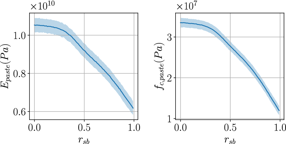
Predictive performance of the learned model corresponding to the homogenization process. The solid line is the predictive mean, and the shaded area is $ \pm 2 $
times standard deviation. The crosses correspond to the noisy observed data.
$ \pm 2 $
times standard deviation. The crosses correspond to the noisy observed data.

Similarly, for the hydration model, Figure 13 shows the learned probabilistic relation between the latent model parameters $ \left({B}_1,{B}_2,\eta, {Q}_{\mathrm{pot}}\right) $
and the ratio
$ \left({B}_1,{B}_2,\eta, {Q}_{\mathrm{pot}}\right) $
and the ratio $ {r}_{\mathrm{sb}} $
. Out of the four available noisy datasets (Section 2.3) for
$ {r}_{\mathrm{sb}} $
. Out of the four available noisy datasets (Section 2.3) for $ T=20{}^{\circ}\mathrm{C} $
, three were used for training and the dataset corresponding to
$ T=20{}^{\circ}\mathrm{C} $
, three were used for training and the dataset corresponding to $ {r}_{\mathrm{sb}}=0.5 $
was used for testing. The value of
$ {r}_{\mathrm{sb}}=0.5 $
was used for testing. The value of $ {E}_a $
was taken from Gruyaert (Reference Gruyaert2011). Figure 15 compares the experimental heat of hydration for different
$ {E}_a $
was taken from Gruyaert (Reference Gruyaert2011). Figure 15 compares the experimental heat of hydration for different $ {r}_{\mathrm{sb}} $
with the probabilistic predictions made using the learned probabilistic model as an input to the hydration model. We observe that the predictions entirely envelop the ground truth data while accounting for the aleatoric noise present in the experimental data. Figure 14a shows the evolution of the entries of the covariance matrix of the conditional on the hydration model latent parameters
$ {r}_{\mathrm{sb}} $
with the probabilistic predictions made using the learned probabilistic model as an input to the hydration model. We observe that the predictions entirely envelop the ground truth data while accounting for the aleatoric noise present in the experimental data. Figure 14a shows the evolution of the entries of the covariance matrix of the conditional on the hydration model latent parameters $ p\left(\boldsymbol{b}|\boldsymbol{x};\boldsymbol{\varphi} \right) $
. It serves as an indicator for the convergence of the VB-EM algorithm. The converged value of the covariance matrix is given by Figure 14b. It confirms the intricate correlation among the hydration model parameters, also reported in Figure B1. This is a general challenge with most physical models that are often overparameterized (at least for a given dataset) leading to multiple configurations of parameters with similar likelihood (see Figure 6).
$ p\left(\boldsymbol{b}|\boldsymbol{x};\boldsymbol{\varphi} \right) $
. It serves as an indicator for the convergence of the VB-EM algorithm. The converged value of the covariance matrix is given by Figure 14b. It confirms the intricate correlation among the hydration model parameters, also reported in Figure B1. This is a general challenge with most physical models that are often overparameterized (at least for a given dataset) leading to multiple configurations of parameters with similar likelihood (see Figure 6).
Learned probabilistic relation between the hydration model parameters and the slag–binder mass ratio $ {r}_{\mathrm{sb}} $
. The solid line denotes the mean, and the shaded area denotes
$ {r}_{\mathrm{sb}} $
. The solid line denotes the mean, and the shaded area denotes $ \pm 2 $
times standard deviation.
$ \pm 2 $
times standard deviation.

(a) Evolution of the entries $ {\phi}_{ij} $
of the lower-triangular matrix
$ {\phi}_{ij} $
of the lower-triangular matrix $ \boldsymbol{L} $
of the covariance matrix (Eq. (2)) with respect to EM iterations. (b) Heat map of the converged value of the covariance matrix
$ \boldsymbol{L} $
of the covariance matrix (Eq. (2)) with respect to EM iterations. (b) Heat map of the converged value of the covariance matrix $ {\boldsymbol{LL}}^T $
of the probabilistic model corresponding to concrete hydration.
$ {\boldsymbol{LL}}^T $
of the probabilistic model corresponding to concrete hydration.

Predictive performance of the learned model corresponding to the hydration process. The solid line is the predictive mean, and the shaded area is $ \pm 2 $
times standard deviation. The crosses correspond to the noisy observed data.
$ \pm 2 $
times standard deviation. The crosses correspond to the noisy observed data.
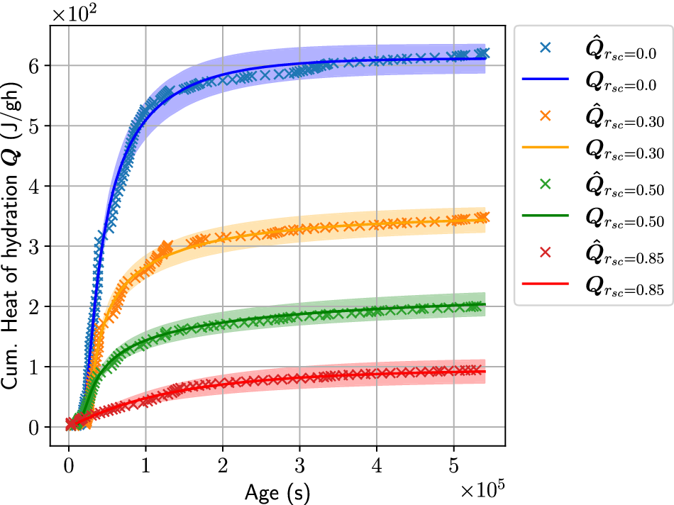
(a) Evolution of the expected objective $ {\unicode{x1D53C}}_{\boldsymbol{b}}\left[\mathcal{O}\right] $
versus the number of iterations. The objective is the GWP of the beam. (b) Evolution of the expected constraints
$ {\unicode{x1D53C}}_{\boldsymbol{b}}\left[\mathcal{O}\right] $
versus the number of iterations. The objective is the GWP of the beam. (b) Evolution of the expected constraints $ {\unicode{x1D53C}}_{\boldsymbol{b}}\left[{\mathcal{C}}_i\right] $
(which should all be negative) versus the number of iterations.
$ {\unicode{x1D53C}}_{\boldsymbol{b}}\left[{\mathcal{C}}_i\right] $
(which should all be negative) versus the number of iterations. $ {\mathcal{C}}_1 $
represents the beam design constraint,
$ {\mathcal{C}}_1 $
represents the beam design constraint, $ {\mathcal{C}}_2 $
represents the temperature constraint, and
$ {\mathcal{C}}_2 $
represents the temperature constraint, and $ {\mathcal{C}}_3 $
gives the demolding time constraint. (c) Trajectory of the design variables (slag–binder mass ratio
$ {\mathcal{C}}_3 $
gives the demolding time constraint. (c) Trajectory of the design variables (slag–binder mass ratio $ {r}_{\mathrm{sb}} $
and the beam height
$ {r}_{\mathrm{sb}} $
and the beam height $ h $
). The red cross represents the optimal value identified upon convergence.
$ h $
). The red cross represents the optimal value identified upon convergence.

Evolution of the standard deviations $ \sigma $
of the design variables to highlight the convergence of the optimization process. We note that the design variables are transformed and scaled in the optimization procedure.
$ \sigma $
of the design variables to highlight the convergence of the optimization process. We note that the design variables are transformed and scaled in the optimization procedure.

At this point, it is crucial to (re)state that the training is performed using indirect, noisy data. It is encouraging to note that the learned models are able to account for the aleatoric uncertainty arising from the noise in the observed data and the epistemic uncertainty due to the finite amount of training data. The probabilistic model is able to learn relationships which were otherwise unavailable in literature, with the aid of physical models and (noisy) data. In this study, the training and validation of the model were somewhat constrained by the limited availability of data, a common challenge in engineering and physics applications. However, this limitation does not detract from the demonstration of our algorithmic framework. In future iterations of this work, an extensive set of experiments can be performed for a larger dataset.
3.2. Optimization results
With the learned probabilistic links as discussed in the previous section, we overcame the issue of forward and backward information flow bottleneck in the workflow connecting the design variables and KPIs relevant for constraints/objective (as discussed in Section 2.4). In this section, we report on the results obtained by performing OUU as discussed in Section 2.6 for the performance-based concrete design workflow. The design variables, objectives, and the constraints are detailed in Table 3. For the temperature constraint, we choose $ {T}_{\mathrm{limit}}=60{}^{\circ}\mathrm{C} $
and for the demolding time constraint, we choose 10 hours. To improve the numerical stability, we scale the variables, constraints, and objectives to make them of the order 1. To demonstrate the optimization scheme proposed, a simply supported beam is used as discussed in Section 1.1, with parameters given in Table D1. Colloquially, we aim to find the value(s) of slag–binder mass ratio
$ {T}_{\mathrm{limit}}=60{}^{\circ}\mathrm{C} $
and for the demolding time constraint, we choose 10 hours. To improve the numerical stability, we scale the variables, constraints, and objectives to make them of the order 1. To demonstrate the optimization scheme proposed, a simply supported beam is used as discussed in Section 1.1, with parameters given in Table D1. Colloquially, we aim to find the value(s) of slag–binder mass ratio $ {r}_{\mathrm{sb}} $
and beam height
$ {r}_{\mathrm{sb}} $
and beam height $ h $
that minimize the objective, on average, while satisfying, on average, the aforementioned constraints.
$ h $
that minimize the objective, on average, while satisfying, on average, the aforementioned constraints.
Physical meaning of the variables used in Figure 8

Physical meaning of the variables/links used in Figure 9

Note. $ \hat{\boldsymbol{x}} $
is the slag–binder mass ratio
$ \hat{\boldsymbol{x}} $
is the slag–binder mass ratio $ {r}_{sb} $
for the all the cases presented above.
$ {r}_{sb} $
for the all the cases presented above.
As discussed, the workflow for estimating the gradient is embarrassingly parallelizable. Hence, for each value considered in the design space, we call the ensemble of the workflows in parallel machines and collect the results. For the subsequent illustrations, a step size of $ 0.05 $
is utilized in the ADAM optimizer and
$ 0.05 $
is utilized in the ADAM optimizer and $ S=100 $
was the number of samples for gradient estimation. We set
$ S=100 $
was the number of samples for gradient estimation. We set $ {\lambda}_i=1\forall i\in \left\{1,\dots, I\right\} $
as the starting value. Figure 16 shows the optimization results. In the design space, we start from values of design variables that violate the beam design constraints
$ {\lambda}_i=1\forall i\in \left\{1,\dots, I\right\} $
as the starting value. Figure 16 shows the optimization results. In the design space, we start from values of design variables that violate the beam design constraints $ {\mathcal{C}}_1 $
as evident from Figure 16b. This activates the corresponding penalty term in the augmented objective (Eq. (14)), thus driving the design variables to satisfy the constraint (around iteration 40). Physically, this implies that the beam is not able to withstand the applied load for the given slag–binder ratio, beam height, and other material parameters (which are kept constant in the optimization procedure). As a result, the optimizer suggests to increase the beam height
$ {\mathcal{C}}_1 $
as evident from Figure 16b. This activates the corresponding penalty term in the augmented objective (Eq. (14)), thus driving the design variables to satisfy the constraint (around iteration 40). Physically, this implies that the beam is not able to withstand the applied load for the given slag–binder ratio, beam height, and other material parameters (which are kept constant in the optimization procedure). As a result, the optimizer suggests to increase the beam height $ h $
in order to satisfy the constraint while also simultaneously increasing the slag–binder mass ratio
$ h $
in order to satisfy the constraint while also simultaneously increasing the slag–binder mass ratio $ {r}_{\mathrm{sb}} $
, owing to the influence of the GWP objective (see Figure 16c). As it can be seen in Figure 16a, this leads to a reduction of the GWP because with the increase of the slag ratio, the Portland cement content, which is mainly responsible for the
$ {r}_{\mathrm{sb}} $
, owing to the influence of the GWP objective (see Figure 16c). As it can be seen in Figure 16a, this leads to a reduction of the GWP because with the increase of the slag ratio, the Portland cement content, which is mainly responsible for the $ {\mathrm{CO}}_2 $
emission, is ultimately reduced. In theory, the optimum value of the slag–binder mass ratio
$ {\mathrm{CO}}_2 $
emission, is ultimately reduced. In theory, the optimum value of the slag–binder mass ratio $ {r}_{\mathrm{sb}} $
approaches one (meaning only slag in the mix) if only the GWP objective with no constraints were to be used in the optimization. But the demolding time constraint
$ {r}_{\mathrm{sb}} $
approaches one (meaning only slag in the mix) if only the GWP objective with no constraints were to be used in the optimization. But the demolding time constraint $ {\mathcal{C}}_3 $
penalizes the objective to limit the slag–binder
$ {\mathcal{C}}_3 $
penalizes the objective to limit the slag–binder $ {r}_{\mathrm{sb}} $
ratio to be around
$ {r}_{\mathrm{sb}} $
ratio to be around $ 0.8 $
(see Figure 16c), since the evolution of mechanical properties is both much faster for Portland cement than for slag and at the same time the absolute values for strength and Young’s modulus are higher. This s also evident in Figure 16b, when around iteration 80, the constraint violation line is crossed thus activating the penalty from
$ 0.8 $
(see Figure 16c), since the evolution of mechanical properties is both much faster for Portland cement than for slag and at the same time the absolute values for strength and Young’s modulus are higher. This s also evident in Figure 16b, when around iteration 80, the constraint violation line is crossed thus activating the penalty from $ {\mathcal{C}}_3 $
. This also stops the nearly linear descent of the GWP objective. In the present illustrations, a value of
$ {\mathcal{C}}_3 $
. This also stops the nearly linear descent of the GWP objective. In the present illustrations, a value of $ 10 $
hours is chosen as the demolding time to demonstrate the procedure. In real-world settings, a manufacturer would be inclined to remove the formwork earlier so that it can be reused. But the lower the requirement of the demolding time, the higher the ratio of cement content required in the mix, leading to an increased hydration heat which in effect accelerates the reaction.
$ 10 $
hours is chosen as the demolding time to demonstrate the procedure. In real-world settings, a manufacturer would be inclined to remove the formwork earlier so that it can be reused. But the lower the requirement of the demolding time, the higher the ratio of cement content required in the mix, leading to an increased hydration heat which in effect accelerates the reaction.
The oscillations in the objective and the constraints as seen in Figure 16a,b are due to the Monte Carlo noise in the gradient estimation. As per Eq. (17), the design variables are treated as random variables following a normal distribution. As discussed in Algorithm 2, the optimization procedure is assumed to converge when the standard deviations $ \sigma $
of the normal distribution attain small values (Figure 17), that is, when the normal degenerates to a Dirac-delta. The
$ \sigma $
of the normal distribution attain small values (Figure 17), that is, when the normal degenerates to a Dirac-delta. The $ \sigma $
values stabilizing to relatively small values points toward the convergence of the algorithm.
$ \sigma $
values stabilizing to relatively small values points toward the convergence of the algorithm.
The performance increase (in terms of GWP) is difficult to evaluate in the current setting. This is due to the fact that the constraint $ {\mathcal{C}}_1 $
is not fulfilled for the initial value of the design variables chosen for the optimization. It is to be highlighted that this is actually an advantage of the method—the user can start with a reasonable design that still violates the constraints. In order to make a reasonable comparison, a design using only Portland cement (i.e.,
$ {\mathcal{C}}_1 $
is not fulfilled for the initial value of the design variables chosen for the optimization. It is to be highlighted that this is actually an advantage of the method—the user can start with a reasonable design that still violates the constraints. In order to make a reasonable comparison, a design using only Portland cement (i.e., $ {r}_{\mathrm{sb}}=0 $
) with only the load-bearing capacity as a constraint (beam design constraint
$ {r}_{\mathrm{sb}}=0 $
) with only the load-bearing capacity as a constraint (beam design constraint $ {\mathcal{C}}_1 $
) and the free parameter being the height of the beam was computed. This minimum height was found to be 77.5 cm with a corresponding GWP of the beam of 1,455
$ {\mathcal{C}}_1 $
) and the free parameter being the height of the beam was computed. This minimum height was found to be 77.5 cm with a corresponding GWP of the beam of 1,455 $ \hskip0.1em {\mathrm{kgCO}}_2\mathrm{eq} $
. Note that this design does not fulfill the temperature constraint
$ \hskip0.1em {\mathrm{kgCO}}_2\mathrm{eq} $
. Note that this design does not fulfill the temperature constraint $ {\mathcal{C}}_2 $
with a maximum temperature of 81°C. Another option for comparison is the first iteration number in the optimization procedure that fulfills all the constraints in expectation, which is the iteration number
$ {\mathcal{C}}_2 $
with a maximum temperature of 81°C. Another option for comparison is the first iteration number in the optimization procedure that fulfills all the constraints in expectation, which is the iteration number $ 30 $
with a GWP of 1,050
$ 30 $
with a GWP of 1,050 $ \hskip0.1em {\mathrm{kgCO}}_2\mathrm{eq} $
. In the subsequent iteration steps, this is further reduced to 900
$ \hskip0.1em {\mathrm{kgCO}}_2\mathrm{eq} $
. In the subsequent iteration steps, this is further reduced to 900 $ \hskip0.1em {\mathrm{kgCO}}_2\mathrm{eq} $
for the optimum value of the design variables obtained in the present study. This reduction in GWP is achieved by increasing the height of the beam to 100
$ \hskip0.1em {\mathrm{kgCO}}_2\mathrm{eq} $
for the optimum value of the design variables obtained in the present study. This reduction in GWP is achieved by increasing the height of the beam to 100 $ \hskip0.1em \mathrm{cm} $
while replacing Portland cement with BFS so that the mass fraction of slag–binder
$ \hskip0.1em \mathrm{cm} $
while replacing Portland cement with BFS so that the mass fraction of slag–binder $ {r}_{\mathrm{sb}} $
is 0.8. The addition of slag to the mixture decreases the strength of the material as illustrated in Figure 12, while at the same time, this decrease is compensated by an increased height. It is also informative to study the evolution of the (expected) constraints shown in Figure 16b. One observes that
$ {r}_{\mathrm{sb}} $
is 0.8. The addition of slag to the mixture decreases the strength of the material as illustrated in Figure 12, while at the same time, this decrease is compensated by an increased height. It is also informative to study the evolution of the (expected) constraints shown in Figure 16b. One observes that $ {\mathcal{C}}_3 $
(green line) associated with the demolding time is the most critical. Thus, in the current example, the GWP could be decreased even further when the time of demolding is extended (depending on the production process of removing the formwork).
$ {\mathcal{C}}_3 $
(green line) associated with the demolding time is the most critical. Thus, in the current example, the GWP could be decreased even further when the time of demolding is extended (depending on the production process of removing the formwork).
4. Conclusion and outlook
We introduced a systematic design approach for the precast concrete industry in the pursuit of sustainable construction practices. It makes use of a holistic optimization framework which combines concrete mixture design with the structural simulation of the precast concrete element within an automated workflow. In this manner, various objectives and constraints, such as the environmental impact of the concrete element or its structural efficiency, can be considered.
The proposed holistic approach is demonstrated on a specific design problem, but should serve as a template that can be readily adapted to other design problems. The advocated black-box stochastic optimization procedure is able to deal with the challenges presented by general workflows, such as the presence of black-box models without derivatives, the effect of uncertainties, and nonlinear constraints. Furthermore, to complete the forward and backward information flow that is essential in the optimization procedure, a method to learn missing (probabilistic) links between the concrete mix design variables and model parameters from experimental data is presented. We note that, to the best of our knowledge, such a link is not available in the literature.
We demonstrated on the precast concrete element the integration of material and structural design in a joint workflow and showcased that this has the potential to decrease the objective, that is, the GWP. For the structural design, semi-analytical models based on the Eurocode are used, whereas the manufacturing process is simulated using a complex FE model. This illustrates the ability of the proposed procedure to combine multiple simulation tools of varying complexity, accounting for different parts of the life cycle. Hence, extending this in order to include, for example, additional load configurations, materials, or life cycle models, is straightforward. The present approach to treat the design process as a workflow, learning the missing links from data/models, and finally using this workflow in a global optimization is transferable to several other material, structural, and mechanical problems. Such extensions could readily include more complex design processes with an increased number of parameters and constraints (the latter due to multiple load configurations or limit states in a real structure). Furthermore, this procedure could be applied to problems involving a complete structure (e.g., bridge and building) instead of a single-element and potentially entailing advanced modeling features that include multiscale models to link material composition to material properties or improve the computation of the GWP using a complete life cycle analysis.
Data availability statement
The code and the data of this study are openly available at the project repository: https://github.com/BAMresearch/LebeDigital.
Acknowledgements
We acknowledge the support of David Alos Shepherd (Building Materials Technology, Karlsruhe Institute of Technology) for digitizing the experimental data. We thank Jonas Nitzler (TUM) for his advice on algorithmic implementations. Our sincere gratitude is extended to the reviewers, whose insightful feedback greatly enhanced the quality of our manuscript.
Author contribution
Conceptualization: P.-S.K., J.F.U.; Software: A.A., E.T.; Visualization: A.A., E.T.; Writing and reviewing code and paper: A.A., E.T., J.F.U.; Writing and reviewing paper: P.-S.K. All authors approved the final submitted draft.
Funding statement
The authors gratefully acknowledge the support of VDI Technologiezentrum GmbH and the Federal Ministry for Education and Research (BMBF) within the collaborative project “Lebenszyklus von Beton—Ontologieentwicklung für die Prozesskette der Betonherstellung.” A.A. and P.-S.K. received support through the subproject “Probabilistic machine learning for the calibration and validation of physics-based models of concrete” (FKZ-13XP5125B). E.T. and J.F.U. received support through the subproject “Ontologien und Workflows für Prozesse, Modelle und Abbildung in Datenbanken” (FKZ-13XP5125B).
Competing interest
The authors declare no competing interests.
Ethical standard
The research meets all ethical guidelines, including adherence to the legal requirements of the study country.
A. Homogenization
A.1. Approximation of elastic properties
The chosen method to homogenize the elastic, isotropic properties $ E $
and
$ E $
and $ \nu $
is the Mori–Tanaka homogenization scheme (Mori and Tanaka, Reference Mori and Tanaka1973). It is a well-established, analytical homogenization method. The formulation uses bulk and shear moduli
$ \nu $
is the Mori–Tanaka homogenization scheme (Mori and Tanaka, Reference Mori and Tanaka1973). It is a well-established, analytical homogenization method. The formulation uses bulk and shear moduli $ K $
and
$ K $
and $ G $
. They are related to
$ G $
. They are related to $ E $
and
$ E $
and $ \nu $
as
$ \nu $
as $ K=\frac{E}{3\left(1-2\nu \right)} $
and
$ K=\frac{E}{3\left(1-2\nu \right)} $
and $ G=\frac{E}{2\left(1+\nu \right)} $
. The used Mori–Tanaka method assumes spherical inclusions in an infinite matrix and considers the interactions of multiple inclusions. The applied formulations follow the notation published in Nežerka and Zeman (Reference Nežerka and Zeman2012) where this method is applied to successfully model the effective concrete stiffness for multiple types of inclusions. The general idea of this analytical homogenization procedure is to describe the overall stiffness of a body
$ G=\frac{E}{2\left(1+\nu \right)} $
. The used Mori–Tanaka method assumes spherical inclusions in an infinite matrix and considers the interactions of multiple inclusions. The applied formulations follow the notation published in Nežerka and Zeman (Reference Nežerka and Zeman2012) where this method is applied to successfully model the effective concrete stiffness for multiple types of inclusions. The general idea of this analytical homogenization procedure is to describe the overall stiffness of a body $ \Omega $
, based on the properties of the individual phases, that is, the matrix and the inclusions. Each of the
$ \Omega $
, based on the properties of the individual phases, that is, the matrix and the inclusions. Each of the $ n $
phases is denoted by the index
$ n $
phases is denoted by the index $ r $
, where
$ r $
, where $ r=0 $
is defined as the matrix phase. The volume fraction of each phase is defined as
$ r=0 $
is defined as the matrix phase. The volume fraction of each phase is defined as
 $$ {c}^{(r)}=\frac{\left\Vert {\Omega}^{(r)}\right\Vert }{\left\Vert \Omega \right\Vert}\hskip1em \mathrm{for}\hskip0.35em r=0,\dots, n. $$
The inclusions are assumed to be spheres, defined by their radius $ {R}^{(r)} $
. The elastic properties of each homogeneous and isotropic phase is given by the material stiffness matrix
$ {R}^{(r)} $
. The elastic properties of each homogeneous and isotropic phase is given by the material stiffness matrix $ {\boldsymbol{L}}^{(r)} $
, here written in terms of the bulk and shear moduli
$ {\boldsymbol{L}}^{(r)} $
, here written in terms of the bulk and shear moduli $ K $
and
$ K $
and $ G $
,
$ G $
,
 $$ {\boldsymbol{L}}^{(r)}=3{K}^{(r)}{\boldsymbol{I}}_{\mathrm{V}}+2{G}^{(r)}{\boldsymbol{I}}_{\mathrm{D}}\hskip1em \mathrm{for}\hskip0.35em r=0,\dots, n, $$
where $ {\boldsymbol{I}}_{\mathrm{V}} $
and
$ {\boldsymbol{I}}_{\mathrm{V}} $
and $ {\boldsymbol{I}}_{\mathrm{D}} $
are the orthogonal projections of the volumetric and deviatoric components.
$ {\boldsymbol{I}}_{\mathrm{D}} $
are the orthogonal projections of the volumetric and deviatoric components.
The method assumes that the micro-heterogeneous body $ \Omega $
is subjected to a macroscale strain
$ \Omega $
is subjected to a macroscale strain $ \boldsymbol{\varepsilon} $
. It is considered that for each phase a concentration factor
$ \boldsymbol{\varepsilon} $
. It is considered that for each phase a concentration factor $ {\boldsymbol{A}}^{(r)} $
can be defined such that
$ {\boldsymbol{A}}^{(r)} $
can be defined such that
 $$ {\boldsymbol{\varepsilon}}^{(r)}={\boldsymbol{A}}^{(r)}\boldsymbol{\varepsilon} \hskip1em \mathrm{for}\hskip0.35em r=0,\dots, n, $$
which computes the average strain $ {\boldsymbol{\varepsilon}}^{(r)} $
within a phase, based on the overall strains. This can then be used to compute the effective stiffness matrix
$ {\boldsymbol{\varepsilon}}^{(r)} $
within a phase, based on the overall strains. This can then be used to compute the effective stiffness matrix $ {\boldsymbol{L}}_{\mathrm{eff}} $
as a volumetric sum over the constituents weighted by the corresponding concentration factor
$ {\boldsymbol{L}}_{\mathrm{eff}} $
as a volumetric sum over the constituents weighted by the corresponding concentration factor
 $$ {\boldsymbol{L}}_{\mathrm{eff}}=\sum \limits_{r=0}^n{c}^{(r)}{\boldsymbol{L}}^{(r)}{\boldsymbol{A}}^{(r)}\hskip1em \mathrm{for}\hskip0.35em r=0,\dots, n. $$
The concentration factors $ {\boldsymbol{A}}^{(r)} $
,
$ {\boldsymbol{A}}^{(r)} $
,
 $$ {\boldsymbol{A}}^{(0)}={\left({c}^{(0)}\boldsymbol{I}+\sum \limits_{r=1}^n{c}^{(r)}{\boldsymbol{A}}_{\mathrm{dil}}^{(r)}\right)}^{-1}, $$
 $$ {\boldsymbol{A}}^{(r)}={\boldsymbol{A}}_{\mathrm{dil}}^{(r)}{\boldsymbol{A}}^{(0)}\hskip1em \mathrm{for}\hskip0.35em r=1,\dots, n, $$
are based on the dilute concentration factors $ {\boldsymbol{A}}_{\mathrm{dil}}^{(r)} $
, which need to be obtained first. The dilute concentration factors are based on the assumption that each inclusion is subjected to the average strain in the matrix
$ {\boldsymbol{A}}_{\mathrm{dil}}^{(r)} $
, which need to be obtained first. The dilute concentration factors are based on the assumption that each inclusion is subjected to the average strain in the matrix $ {\boldsymbol{\varepsilon}}^{(0)} $
; therefore,
$ {\boldsymbol{\varepsilon}}^{(0)} $
; therefore,
 $$ {\boldsymbol{\varepsilon}}^{(r)}={\boldsymbol{A}}_{\mathrm{dil}}^{(r)}{\boldsymbol{\varepsilon}}^{(0)}\hskip1em \mathrm{for}\hskip0.35em r=1,\dots, n. $$
The dilute concentration factors neglect the interaction among phases and are only defined for the inclusion phases $ r=1,\dots, n $
. The applied formulation uses an additive volumetric–deviatoric split, where
$ r=1,\dots, n $
. The applied formulation uses an additive volumetric–deviatoric split, where
 $$ {\boldsymbol{A}}_{\mathrm{dil}}^{(r)}={A}_{\mathrm{dil},\mathrm{V}}^{(r)}{\boldsymbol{I}}_{\mathrm{V}}+{A}_{\mathrm{dil},\mathrm{D}}^{(r)}{\boldsymbol{I}}_{\mathrm{D}}\hskip1em \mathrm{for}\hskip0.35em r=1,\dots, n,\hskip1em \mathrm{with} $$
 $$ {A}_{\mathrm{dil},\mathrm{V}}^{(r)}=\frac{K^{(0)}}{K^{(0)}+{\alpha}^{(0)}\left({K}^{(r)}-{K}^{(0)}\right)}, $$
 $$ {A}_{\mathrm{dil},\mathrm{D}}^{(r)}=\frac{G^{(0)}}{G^{(0)}+{\beta}^{(0)}\left({G}^{(r)}-{G}^{(0)}\right)}. $$
The auxiliary factors follow from the Eshelby solution as
 $$ {\alpha}^{(0)}=\frac{1+{\nu}^{(0)}}{3\left(1+{\nu}^{(0)}\right)}\hskip1em \mathrm{and}\hskip1em {\beta}^{(0)}=\frac{2\left(4-5{\nu}^{(0)}\right)}{15\left(1-{\nu}^{(0)}\right)}, $$
where $ {\nu}^{(0)} $
refers to the Poission ratio of the matrix phase. The effective bulk and shear moduli can be computed based on a sum over the phases
$ {\nu}^{(0)} $
refers to the Poission ratio of the matrix phase. The effective bulk and shear moduli can be computed based on a sum over the phases
 $$ {K}_{\mathrm{eff}}=\frac{c^{(0)}{K}^{(0)}+{\sum}_{r=1}^n{c}^{(r)}{K}^{(r)}{A}_{\mathrm{dil},\mathrm{V}}^{(r)}}{c^{(0)}+{\sum}_{r=1}^n{c}^{(r)}{A}_{\mathrm{dil},\mathrm{V}}^{(r)}}, $$
 $$ {G}_{\mathrm{eff}}=\frac{c^{(0)}{G}^{(0)}+{\sum}_{r=1}^n{c}^{(r)}{G}^{(r)}{A}_{\mathrm{dil},\mathrm{D}}^{(r)}}{c^{(0)}+{\sum}_{r=1}^n{c}^{(r)}{A}_{\mathrm{dil},\mathrm{D}}^{(r)}}. $$
Based on the concept of Eq. (A3), with the formulations (Eqs. (A2), (A4), and (A5)), the average matrix stress is defined as
 $$ {\boldsymbol{\sigma}}^{(0)}={\boldsymbol{L}}^{(0)}{\boldsymbol{A}}^{(0)}{{\boldsymbol{L}}_{\mathrm{eff}}}^{-1}\boldsymbol{\sigma} . $$
A.1.1. Approximation of compressive strength
The estimation of the concrete compressive strength $ {f}_c $
follows the ideas of Nežerka et al. (Reference Nežerka, Hrbek, Prošek, Somr, Tesárek and Fládr2018). The procedure here is taken from the code provided in the link in Nežerka and Zeman (Reference Nežerka and Zeman2012). The assumption is that a failure in the cement paste will cause the concrete to crack. The approach is based on two main assumptions. First, the Mori–Tanaka method is used to estimate the average stress within the matrix material
$ {f}_c $
follows the ideas of Nežerka et al. (Reference Nežerka, Hrbek, Prošek, Somr, Tesárek and Fládr2018). The procedure here is taken from the code provided in the link in Nežerka and Zeman (Reference Nežerka and Zeman2012). The assumption is that a failure in the cement paste will cause the concrete to crack. The approach is based on two main assumptions. First, the Mori–Tanaka method is used to estimate the average stress within the matrix material $ {\boldsymbol{\sigma}}^{(m)} $
. The formulation is given in Eq. (A14). Second, the von Mises failure criterion of the average matrix stress is used to estimate the uniaxial compressive strength
$ {\boldsymbol{\sigma}}^{(m)} $
. The formulation is given in Eq. (A14). Second, the von Mises failure criterion of the average matrix stress is used to estimate the uniaxial compressive strength
 $$ {f}_c=\sqrt{3{J}_2}, $$
with $ {J}_2\left(\boldsymbol{\sigma} \right)=\frac{1}{2}{\boldsymbol{\sigma}}_{\mathrm{D}}:{\boldsymbol{\sigma}}_{\mathrm{D}} $
and
$ {J}_2\left(\boldsymbol{\sigma} \right)=\frac{1}{2}{\boldsymbol{\sigma}}_{\mathrm{D}}:{\boldsymbol{\sigma}}_{\mathrm{D}} $
and $ {\boldsymbol{\sigma}}_{\mathrm{D}}=\boldsymbol{\sigma} -\frac{1}{3}\mathrm{trace}\left(\boldsymbol{\sigma} \right)\boldsymbol{I} $
. It is achieved by finding a uniaxial macroscopic stress
$ {\boldsymbol{\sigma}}_{\mathrm{D}}=\boldsymbol{\sigma} -\frac{1}{3}\mathrm{trace}\left(\boldsymbol{\sigma} \right)\boldsymbol{I} $
. It is achieved by finding a uniaxial macroscopic stress $ \boldsymbol{\sigma} ={\left[\begin{array}{cccccc}-{f}_{c,\mathrm{eff}}& 0& 0& 0& 0& 0\end{array}\right]}^{\mathrm{T}} $
, which exactly fulfills the von Mises failure criterion (Eq. (A15)) for the average stress within the matrix
$ \boldsymbol{\sigma} ={\left[\begin{array}{cccccc}-{f}_{c,\mathrm{eff}}& 0& 0& 0& 0& 0\end{array}\right]}^{\mathrm{T}} $
, which exactly fulfills the von Mises failure criterion (Eq. (A15)) for the average stress within the matrix $ {\boldsymbol{\sigma}}^{(m)} $
. The procedure here is taken from the code provided in the link in Nežerka and Zeman (Reference Nežerka and Zeman2012). First, a
$ {\boldsymbol{\sigma}}^{(m)} $
. The procedure here is taken from the code provided in the link in Nežerka and Zeman (Reference Nežerka and Zeman2012). First, a $ {J}_2^{\mathrm{test}} $
is computed for a uniaxial test stress
$ {J}_2^{\mathrm{test}} $
is computed for a uniaxial test stress $ {\boldsymbol{\sigma}}^{\mathrm{test}}={\left[\begin{array}{cccccc}{f}^{\mathrm{test}}& 0& 0& 0& 0& 0\end{array}\right]}^{\mathrm{T}} $
. Then the matrix stress
$ {\boldsymbol{\sigma}}^{\mathrm{test}}={\left[\begin{array}{cccccc}{f}^{\mathrm{test}}& 0& 0& 0& 0& 0\end{array}\right]}^{\mathrm{T}} $
. Then the matrix stress $ {\boldsymbol{\sigma}}^{(m)} $
is computed based on the test stress following Eq. (A14). This is used to compute the second deviatoric stress invariant
$ {\boldsymbol{\sigma}}^{(m)} $
is computed based on the test stress following Eq. (A14). This is used to compute the second deviatoric stress invariant $ {J}_2^{(m)} $
for the average matrix stress. Finally, the effective compressive strength is estimated as
$ {J}_2^{(m)} $
for the average matrix stress. Finally, the effective compressive strength is estimated as
 $$ {f}_{\mathrm{c}, eff}=\frac{J_2^{\mathrm{test}}}{J_2^{(m)}}{f}^{\mathrm{test}}. $$
A.1.2. Approximation of thermal conductivity
Homogenization of the thermal conductivity is based on the Mori–Tanaka method as well. The formulation is similar to Eqs. (A12) and (A13). The expressions are taken from Stránský et al. (Reference Stránský, Vorel, Zeman and Šejnoha2011). The thermal conductivity $ {\chi}_{\mathrm{eff}} $
is computed as
$ {\chi}_{\mathrm{eff}} $
is computed as
 $$ {\chi}_{\mathrm{eff}}=\frac{c^{(m)}{\chi}^{(m)}+{c}^{(i)}{\chi}^{(i)}{A}_{\chi}^{(i)}}{c^{(m)}+{c}^{(i)}{A}_{\chi}^{(i)}}\hskip1em \mathrm{and} $$
 $$ {A}_{\chi}^{(i)}=\frac{3{\chi}^{(m)}}{2{\chi}^{(m)}+{\chi}^{(i)}}. $$
B. FE concrete model
B.1. Modeling of the temperature field
The temperature distribution is generally described by the heat equation as
 $$ \rho C\frac{\partial T}{\partial t}=\nabla \cdot \left(\lambda \nabla T\right)+\frac{\partial Q}{\partial t} $$
with $ \lambda $
the effective thermal conductivity,
$ \lambda $
the effective thermal conductivity, $ C $
the specific heat capacity,
$ C $
the specific heat capacity, $ \rho $
the density, and
$ \rho $
the density, and $ \rho C $
the volumetric heat capacity. The volumetric heat
$ \rho C $
the volumetric heat capacity. The volumetric heat $ Q $
due to hydration is also called the latent heat of hydration, or the heat source. In this article, the density, the thermal conductivity, and the volumetric heat capacity to be constants are assumed to be sufficiently accurate for our purpose, even though there are more elaborate models taking into account the effects of temperature, moisture, and/or the hydration.
$ Q $
due to hydration is also called the latent heat of hydration, or the heat source. In this article, the density, the thermal conductivity, and the volumetric heat capacity to be constants are assumed to be sufficiently accurate for our purpose, even though there are more elaborate models taking into account the effects of temperature, moisture, and/or the hydration.
B.1.1.
Degree of hydration
$ \alpha $

The DOH $ \alpha $
is defined as the ratio between the cumulative heat
$ \alpha $
is defined as the ratio between the cumulative heat $ Q $
at time
$ Q $
at time $ t $
and the total theoretical volumetric heat by complete hydration
$ t $
and the total theoretical volumetric heat by complete hydration $ {Q}_{\infty } $
:
$ {Q}_{\infty } $
:
 $$ \alpha (t)=\frac{Q(t)}{Q_{\infty }}, $$
assuming a linear relation between the DOH and the heat development. Therefore, the time derivative of the heat source $ \dot{Q} $
can be rewritten in terms of
$ \dot{Q} $
can be rewritten in terms of $ \alpha $
,
$ \alpha $
,
 $$ \frac{\partial Q}{\partial t}=\frac{\partial \alpha }{\partial t}{Q}_{\infty }. $$
Approximated values for the total potential heat range between 300 and 600 J/g for binders of different cement types, for example, OPC $ {Q}_{\infty }=375\hbox{--} 525\hskip0.1em \mathrm{J}/\mathrm{g} $
or Pozzolanic cement
$ {Q}_{\infty }=375\hbox{--} 525\hskip0.1em \mathrm{J}/\mathrm{g} $
or Pozzolanic cement $ {Q}_{\infty }=315\hbox{--} 420\hskip0.22em $
J/g.
$ {Q}_{\infty }=315\hbox{--} 420\hskip0.22em $
J/g.
B.1.2. Affinity
The heat release can be modeled based on the chemical affinity $ A $
of the binder. The hydration kinetics are defined as a function of affinity at a reference temperature
$ A $
of the binder. The hydration kinetics are defined as a function of affinity at a reference temperature $ \tilde{A} $
and a temperature dependent scale factor
$ \tilde{A} $
and a temperature dependent scale factor $ a $
$ a $
 $$ \dot{\alpha}=\tilde{A}\left(\alpha \right)a(T). $$
The reference affinity, based on the DOH, is approximated by
 $$ \tilde{A}\left(\alpha \right)={B}_1\left(\frac{B_2}{\alpha_{\mathrm{max}}}+\alpha \right)\left({\alpha}_{\mathrm{max}}-\alpha \right)\exp \left(-\eta \frac{\alpha }{\alpha_{\mathrm{max}}}\right), $$
where $ {B}_1 $
and
$ {B}_1 $
and $ {B}_2 $
are coefficients depending on the binder. The scale function is given as
$ {B}_2 $
are coefficients depending on the binder. The scale function is given as
 $$ a=\exp \left(-\frac{E_a}{R}\left(\frac{1}{T}-\frac{1}{T_{\mathrm{ref}}}\right)\right). $$
An example function to approximate the maximum DOH based on the water to cement mass ratio $ {r}_{\mathrm{wc}} $
, by Mills (Reference Mills1966), is the following:
$ {r}_{\mathrm{wc}} $
, by Mills (Reference Mills1966), is the following:
 $$ {\alpha}_{\mathrm{max}}=\frac{1.031{r}_{\mathrm{wc}}}{0.194+{r}_{\mathrm{wc}}}. $$
This refers to Portland cement. Figure B1 shows the influence of the three numerical parameters $ {B}_1 $
,
$ {B}_1 $
, $ {B}_2 $
,
$ {B}_2 $
, $ \eta $
and the potential heat release
$ \eta $
and the potential heat release $ {Q}_{\infty } $
on the heat release rate as well as on the cumulative heat release.
$ {Q}_{\infty } $
on the heat release rate as well as on the cumulative heat release.
Influence of the hydration parameters on the heat release rate and the cumulative heat release.
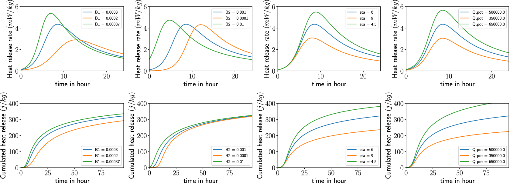
B.1.3. Discretization and solution
Using Eq. (B3) in Eq. (B1), the heat equation is given as
 $$ \rho C\frac{\partial T}{\partial t}=\nabla \cdot \left(\lambda \nabla T\right)+{Q}_{\infty}\frac{\partial \alpha }{\partial t}. $$
Now we apply a backward Euler scheme
 $$ \dot{T}=\frac{T^{n+1}-{T}^n}{\Delta t}\hskip1em \mathrm{and} $$
 $$ \dot{\alpha}=\frac{\Delta \alpha }{\Delta t}\hskip1em \mathrm{with}\hskip1em \Delta \alpha ={\alpha}^{n+1}-{\alpha}^n $$
and drop the index $ n+1 $
for readability to obtain
$ n+1 $
for readability to obtain
 $$ \rho CT-\Delta t\nabla \cdot \left(\lambda \nabla T\right)-{Q}_{\infty}\Delta \alpha =\rho {CT}^n. $$
Using Eqs. (B10) and (B4), a formulation for $ \Delta \alpha $
is obtained:
$ \Delta \alpha $
is obtained:
 $$ \Delta \alpha =\Delta t\tilde{A}\left(\alpha \right)a(T). $$
We define the affinity in terms of $ {\alpha}^n $
and
$ {\alpha}^n $
and $ \Delta \alpha $
to solve for
$ \Delta \alpha $
to solve for $ \Delta \alpha $
on the quadrature point level
$ \Delta \alpha $
on the quadrature point level
 $$ \tilde{A}={B}_1\exp \left(-\eta \frac{\Delta \alpha +{\alpha}^n}{\alpha_{\mathrm{max}}}\right)\left(\frac{B_2}{\alpha_{\mathrm{max}}}+\Delta \alpha +{\alpha}^n\right)\cdot \left({\alpha}_{\mathrm{max}}-\Delta \alpha -{\alpha}^n\right). $$
Now we can solve the nonlinear function
 $$ f\left(\Delta \alpha \right)=\Delta \alpha -\Delta t\tilde{A}\left(\Delta \alpha \right)a(T)=0 $$
using an iterative Newton–Raphson solver.
B.2. Coupling material properties to degree of hydration
B.2.1. Compressive strength
The compressive strength in terms of the DOH can be approximated using an exponential function (cf. Carette and Staquet, Reference Carette and Staquet2016):
 $$ {f}_{\mathrm{c}}\left(\alpha \right)=\alpha {(t)}^{a_{f_{\mathrm{c}}}}{f}_{\mathrm{c}\infty }. $$
This model has two parameters, $ {f}_{\mathrm{c}\infty } $
, the compressive strength of the parameter at full hydration,
$ {f}_{\mathrm{c}\infty } $
, the compressive strength of the parameter at full hydration, $ \alpha =1 $
, and
$ \alpha =1 $
, and $ {a}_{f_{\mathrm{c}}} $
the exponent, which is a material parameter that characterizes the temporal evolution.
$ {a}_{f_{\mathrm{c}}} $
the exponent, which is a material parameter that characterizes the temporal evolution.
The first parameter could theoretically be obtained through experiments. However, the total hydration can take years. Therefore, we can compute it using the 28 days values of the compressive strength and the corresponding DOH:
 $$ {f}_{\mathrm{c}\infty }=\frac{f_{\mathrm{c}28}}{{\alpha_{28}}^{a_{f_{\mathrm{c}}}}}. $$
B.2.2. Young’s modulus
The publication (Carette and Staquet, Reference Carette and Staquet2016) proposes a model for the evolution of the Young modulus assuming an initial linear increase of the Young modulus up to a DOH $ {\alpha}_t $
:
$ {\alpha}_t $
:
 $$ E\left(\alpha \right)=\left\{\begin{array}{ll}{E}_{\infty}\frac{\alpha (t)}{\alpha_t}{\alpha_t}^{a_E}& \mathrm{for}\hskip0.35em \alpha <{\alpha}_t\\ {}{E}_{\infty}\alpha {(t)}^{a_E}& \mathrm{for}\hskip0.35em \alpha \ge {\alpha}_t.\end{array}\right. $$
Contrary to other publications, no dormant period is assumed. Similarly to the strength standardized testing of the Young modulus is done after 28 days, $ {E}_{28} $
. To effectively use these experimental values,
$ {E}_{28} $
. To effectively use these experimental values, $ {E}_{\infty } $
is approximated as
$ {E}_{\infty } $
is approximated as
 $$ {E}_{\infty }=\frac{E_{28}}{{\alpha_{28}}^{a_E}}, $$
using the approximated DOH.
B.3. Constraints
The FEM simulation is used to compute two practical constraints relevant to the precast concrete industry. At each time step, the worst point is chosen to represent the part, therefore ensuring that the criterion is fulfilled in the whole domain. The first constraint limits the maximum allowed temperature. The constraint is computed as the normalized difference between the maximum temperature reached $ {T}_{\mathrm{max}} $
and the temperature limit
$ {T}_{\mathrm{max}} $
and the temperature limit $ {T}_{\mathrm{limit}} $
 $$ {\mathcal{C}}_{\mathrm{T}}=\frac{T_{\mathrm{max}}-{T}_{\mathrm{limit}}}{T_{\mathrm{limit}}}, $$
where $ {\mathcal{C}}_{\mathrm{T}}>0 $
is not admissible, as the temperature limit 60°C has been exceeded.
$ {\mathcal{C}}_{\mathrm{T}}>0 $
is not admissible, as the temperature limit 60°C has been exceeded.
The second constraint is the estimated time of demolding. This is critical, as the manufacturer has a limited number of forms. The faster the part can be demolded, the faster it can be reused, increasing the output capacity. On the other hand, the part must not be demolded too early, as it might get damaged while being moved. To approximate the minimal time of demolding, a constraint is formulated based on the local stresses $ {\mathcal{C}}_{\sigma } $
. It evaluates the Rankine criterion for the principal tensile stresses, using the yield strength of steel
$ {\mathcal{C}}_{\sigma } $
. It evaluates the Rankine criterion for the principal tensile stresses, using the yield strength of steel $ {f}_{\mathrm{yk}} $
and a simplified Drucker–Prager criterion, based on the evolving compressive strength of the concrete
$ {f}_{\mathrm{yk}} $
and a simplified Drucker–Prager criterion, based on the evolving compressive strength of the concrete $ {f}_c $
,
$ {f}_c $
,
 $$ {\mathcal{C}}_{\sigma }=\max \left\{\begin{array}{l}{\mathcal{C}}_{\mathrm{RK}}=\frac{\parallel {\sigma}_t^{\prime}\parallel -{f}_{\mathrm{yk}}}{f_{\mathrm{yk}}}\\ {}{\mathcal{C}}_{\mathrm{DP}}=\frac{\sqrt{\frac{1}{2}{I}_1^2-{I}_2}-\frac{f_c^3}{\sqrt{3}}}{f_c}\end{array}\right., $$
where $ {\mathcal{C}}_{\sigma }>0 $
is not admissible. In contrast to standard yield surfaces, the value is normalized, to be unit less. This constraint aims to approximate the compressive failure often simulated with plasticity and the tensile effect of reinforcement steel. As boundary conditions, a simply supported beam under its own weight has been chosen to approximate possible loading conditions while the part is moved. This constraint is evaluated for each time step in the simulation. The critical point in time is approximated where
$ {\mathcal{C}}_{\sigma }>0 $
is not admissible. In contrast to standard yield surfaces, the value is normalized, to be unit less. This constraint aims to approximate the compressive failure often simulated with plasticity and the tensile effect of reinforcement steel. As boundary conditions, a simply supported beam under its own weight has been chosen to approximate possible loading conditions while the part is moved. This constraint is evaluated for each time step in the simulation. The critical point in time is approximated where $ {\mathcal{C}}_{\sigma}\left({t}_{\mathrm{crit}}\right)=0 $
. This is normalized with the prescribed time of demolding to obtain a dimensionless constraint.
$ {\mathcal{C}}_{\sigma}\left({t}_{\mathrm{crit}}\right)=0 $
. This is normalized with the prescribed time of demolding to obtain a dimensionless constraint.
C. Beam design
We follow the design code (DIN EN 1992-1-1, 2011) for a singly reinforced beam, which is a reinforced concrete beam with reinforcement only at the bottom. The assumed cross-section is rectangular.
C.1. Maximum bending moment
Assuming a simply supported beam with a given length $ l $
in millimeters, a distributed load
$ l $
in millimeters, a distributed load $ q $
in Newton per millimeters and a point load
$ q $
in Newton per millimeters and a point load $ F $
in Newton per millimeters, the maximum bending moment
$ F $
in Newton per millimeters, the maximum bending moment $ {M}_{\mathrm{max}} $
in Newton per square millimeter is computed as
$ {M}_{\mathrm{max}} $
in Newton per square millimeter is computed as
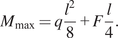 $$ {M}_{\mathrm{max}}=q\frac{l^2}{8}+F\frac{l}{4}. $$
The applied loads already incorporate any required safety factors.
C.2. Computing the minimal required steel reinforcement
Given a beam with the height $ h $
in millimeters, a concrete cover of
$ h $
in millimeters, a concrete cover of $ c $
in millimeters, a steel reinforcement diameter of
$ c $
in millimeters, a steel reinforcement diameter of $ d $
in millimeters for the longitudinal bars, and a bar diameter of
$ d $
in millimeters for the longitudinal bars, and a bar diameter of $ d $
in millimeters for the transversal reinforcement also called stirrups,
$ d $
in millimeters for the transversal reinforcement also called stirrups,
 $$ {h}_{\mathrm{eff}}=h-c-{d}_{\mathrm{st}}-\frac{1}{2}d. $$
According to the German norm standard safety factors are applied, $ {\alpha}_{\mathrm{cc}}=0.85 $
,
$ {\alpha}_{\mathrm{cc}}=0.85 $
, $ {\gamma}_c=1.5 $
, and
$ {\gamma}_c=1.5 $
, and $ {\gamma}_s=1.15 $
, leading to the design compressive strength for concrete
$ {\gamma}_s=1.15 $
, leading to the design compressive strength for concrete $ {f}_{\mathrm{cd}} $
and the design tensile yield strength
$ {f}_{\mathrm{cd}} $
and the design tensile yield strength $ {f}_{\mathrm{ywd}} $
for steel
$ {f}_{\mathrm{ywd}} $
for steel
 $$ {f}_{\mathrm{c}\mathrm{d}}={\alpha}_{\mathrm{c}\mathrm{c}}\frac{f_{\mathrm{c}}}{\gamma_{\mathrm{c}}}, $$
 $$ {f}_{\mathrm{ywd}}=\frac{f_{\mathrm{yk}}}{\gamma_{\mathrm{s}}}, $$
where $ {f}_c $
denotes the concrete compressive strength and
$ {f}_c $
denotes the concrete compressive strength and $ {f}_{\mathrm{yk}} $
the steel’s tensile yield strength.
$ {f}_{\mathrm{yk}} $
the steel’s tensile yield strength.
To compute the force applied in the compression zone, the lever arm of the applied moment $ z $
is given by
$ z $
is given by
 $$ z={h}_{\mathrm{eff}}\left(0.5+\sqrt{0.25-0.5\mu}\right),\hskip1em \mathrm{with} $$
 $$ \mu =\frac{M_{\mathrm{max}}}{bh_{\mathrm{eff}}^2{f}_{\mathrm{cd}}}. $$
The minimum required steel $ {A}_{s,\mathrm{req}} $
is then computed based on the lever arm, the design yield strength of steel and the maximum bending moment, as
$ {A}_{s,\mathrm{req}} $
is then computed based on the lever arm, the design yield strength of steel and the maximum bending moment, as
 $$ {A}_{s,\mathrm{req}}=\frac{M_{\mathrm{max}}}{f_{\mathrm{ywd}}z}. $$
C.3. Optimization constraints
C.3.1. Compressive strength constraint
Based on Eq. (C6), we define the compressive strength constraint as
 $$ {\mathcal{C}}_{\mathrm{fc}}=\mu -0.5, $$
where $ {\mathcal{C}}_{\mathrm{fc}}>0 $
is not admissible, as there is no solution for Eq. (C6).
$ {\mathcal{C}}_{\mathrm{fc}}>0 $
is not admissible, as there is no solution for Eq. (C6).
C.3.2. Geometrical constraint
The geometrical constraint checks that the required steel area $ {A}_{s,\mathrm{req}} $
does not exceed the maximum steel area
$ {A}_{s,\mathrm{req}} $
does not exceed the maximum steel area $ {A}_{s,\max } $
that fits inside the design space. For our example, we assume the steel reinforcement is only arranged in a single layer. This limits the available space for rebars in two ways, by the required minimal spacing
$ {A}_{s,\max } $
that fits inside the design space. For our example, we assume the steel reinforcement is only arranged in a single layer. This limits the available space for rebars in two ways, by the required minimal spacing $ {s}_{\mathrm{min}} $
between the bars, to allow concrete to pass, and by the required space on the outside, the concrete cover
$ {s}_{\mathrm{min}} $
between the bars, to allow concrete to pass, and by the required space on the outside, the concrete cover $ c $
, and stirrups diameter
$ c $
, and stirrups diameter $ {d}_{\mathrm{st}} $
. To compute
$ {d}_{\mathrm{st}} $
. To compute $ {A}_{s,\max } $
, the maximum number for steel bars
$ {A}_{s,\max } $
, the maximum number for steel bars $ {n}_{s,\max } $
and the maximum diameter
$ {n}_{s,\max } $
and the maximum diameter $ {d}_{\mathrm{max}} $
from a given list of admissible diameters are determined that fulfill
$ {d}_{\mathrm{max}} $
from a given list of admissible diameters are determined that fulfill
 $$ s\ge {s}_{\mathrm{min}},\hskip1em \mathrm{with} $$
 $$ s=\frac{b-2c-2{d}_{\mathrm{st}}-{n}_{s,\max }{d}_{\mathrm{max}}}{n_{s,\max }-1}\hskip1em \mathrm{and} $$
 $$ {n}_{s,\max}\ge 2. $$
According to DIN1992-1-1 (2011), the minimum spacing between two bars $ {s}_{\mathrm{min}} $
is given by the minimum of the concrete cover (2.5 cm) and the rebar diameter. The maximum possible reinforcement is given by
$ {s}_{\mathrm{min}} $
is given by the minimum of the concrete cover (2.5 cm) and the rebar diameter. The maximum possible reinforcement is given by
 $$ {A}_{s,\max }={n}_s\pi {\left(\frac{d}{2}\right)}^2. $$
The geometry constraint is computed as
 $$ {\mathcal{C}}_g=\frac{A_{s,\mathrm{req}}-{A}_{s,\max }}{A_{s,\max }}, $$
where $ {\mathcal{C}}_g>0 $
is not admissible, as the required steel area exceeds the available space.
$ {\mathcal{C}}_g>0 $
is not admissible, as the required steel area exceeds the available space.
C.3.3. Combined beam constraint
To simplify the optimization procedure, the two constraints are combined into a single one by using the maximum value:
 $$ {\mathcal{C}}_{\mathrm{beam}}=\max \left({\mathcal{C}}_g,{\mathcal{C}}_{\mathrm{fc}}\right). $$
Evidently, this constraint is also defined as: $ {\mathcal{C}}_{\mathrm{beam}}>0 $
is not admissible.
$ {\mathcal{C}}_{\mathrm{beam}}>0 $
is not admissible.
D. Parameter tables
This is the collection of the used parameters for the various example calculations.
Parameters of the simply supported beam for the computation of the steel reinforcement


 Open access
Comments
No Comments have been published for this article.