




Introduction
Radiocarbon 14C is a radioactive isotope produced by cosmic rays in the Earth’s atmosphere and used to determine the age of carbon-based samples, which forms a basis for precise archaeology. Initially, it was assumed that the production rate of radiocarbon is constant in time, and the so-called 14C age represents the true calendar age. However, it was soon found that the 14C production rate and its relative concentration vary over time, as modulated by geomagnetic shielding, solar activity, and climate. To account for that, a calibrationcurve approach has been developed as presented in a community consensus IntCal dataset (Reimer et al. Reference Reimer, Austin, Bard, Bayliss, Blackwell, Ramsey, Butzin, Cheng, Edwards, Friedrich, Grootes, Guilderson, Hajdas, Heaton, Hogg, Hughen, Kromer, Manning, Muscheler and Talamo2020). Since these changes are assumed to be slow, the IntCal curve presents a slightly smoothed 14C dataset with a 5–10-year time resolution. However, it may sometimes lead to somewhat ambiguous and not very precise dating. To account for the variable production of 14C, a carbon-cycle model needs to be applied to relate the production rate to the measured concentrations. Radiocarbon production and transport in the atmosphere are typically modeled by applying a box model with fixed geometry, which works well for slow changes (e.g., Bard et al. Reference Bard, Raisbeck, Yiou and Jouzel1997; Büntgen et al. Reference Büntgen, Wacker, Galván, Arnold, Arseneault, Baillie, Beer, Bernabei, Bleicher, Boswijk, Bräuning, Carrer, Ljungqvist, Cherubini, Christl, Christie, Clark, Cook, D’Arrigo and Young2018; Oeschger et al. Reference Oeschger, Siegenthaler, Schotterer and Gugelmann1975).
As discovered by Miyake et al. (Reference Miyake, Nagaya, Masuda and Nakamura2012), very rarely, radiocarbon concentration can exhibit strong, well-identifiable spikes in Δ14C corresponding to a nearly instant production of a large amount of 14C in the atmosphere. Such spikes, commonly called “Miyake events,” offer unique time stamps, making the absolute dating of samples covering the corresponding time periods possible (Heaton et al. Reference Heaton, Bard, Bayliss, Blaauw, Bronk Ramsey, Reimer, Turney and Usoskin2024). Accordingly, it is crucially important to study the Miyake events with the highest possible precision and to understand their nature (Usoskin et al. Reference Usoskin, Miyake, Baroni, Brehm, Dalla, Hayakawa, Hudson, Jull, Knipp, Koldobskiy, Maehara, Mekhaldi, Notsu, Poluianov, Rozanov, Shapiro, Spiegl, Sukhodolov, Uusitalo and Wacker2023).
Here we present a new approach to model fast changes of radiocarbon production and transport in the atmosphere, by utilizing a full and precise 3D plus time modeling of the atmospheric dynamics, by using the chemistry-climate SOCOL:14C-Ex model (Golubenko et al. Reference Golubenko, Usoskin, Rozanov and Bard2025). We describe the model and its application to the known Miyake events to demonstrate its accuracy.
Miyake events as manifestations of extreme solar particle events
Miyake et al. (Reference Miyake, Nagaya, Masuda and Nakamura2012) discovered a sudden strong increase of about 12‰ (subsequent studies refined this estimate of about 18–20‰ [2023]), in Δ14C corresponding to the year AD 775 (1175 BP). Miyake discussed both a supernova explosion and a solar origin as possible causes of the event; however, they did not identify either as the definitive source. They concluded that, with the present knowledge, the cause of the event cannot be specified. Only gamma-ray emission from a supernova explosion can produce such a short spike (Pavlov et al. Reference Pavlov, Blinov, Konstantinov, Ostryakov, Vasilyev, Vdovina and Volkov2013), while a cosmic-ray signal would have been diluted over centuries or millennia due to the diffusive cosmic-ray transport in the interstellar medium. However, it was soon demonstrated (Usoskin et al. Reference Usoskin, Kromer, Ludlow, Beer, Friedrich, Kovaltsov, Solanki and Wacker2013) that the enhanced production of 14C was likely caused by an enormous burst of solar energetic particles, named ESPE (extreme solar particle event). As discussed by Pavlov et al. (Reference Pavlov, Blinov, Konstantinov, Ostryakov, Vasilyev, Vdovina and Volkov2013), while a gamma-ray pulse from a supernova or a galactic gamma-ray burst can potentially produce radiocarbon in the Earth’s atmosphere, it cannot create a measurable amount of another cosmogenic isotope 10Be there. Clear detection of a 10Be spike, dated to AD 775 (1175 BP), in both Greenland and Antarctic ice cores (e.g., Mekhaldi et al. Reference Mekhaldi, Muscheler, Adolphi, Aldahan, Beer, McConnell, Possnert, Sigl, Svensson, Synal, Welten and Woodruff2015; Sukhodolov et al. Reference Sukhodolov, Usoskin, Rozanov, Asvestari, Ball, Curran, Fischer, Kovaltsov, Miyake, Peter, Plummer, Schmutz, Severi and Traversi2017; Usoskin et al. Reference Usoskin, Kromer, Ludlow, Beer, Friedrich, Kovaltsov, Solanki and Wacker2013) excluded gamma-rays as a potential source of the Miyake event. Other non-solar sources, such as a cometary impact on Earth (Liu et al. Reference Liu, Zhang, Peng, Ling, Shen, Liu, Sun, Shen, Liu and Sun2014), have also been excluded by a careful analysis of available data (Usoskin and Kovaltsov, Reference Usoskin and Kovaltsov2015). More such cosmogenic isotope spikes have been discovered since (e.g., Bard et al. Reference Bard, Miramont, Capano, Guibal, Marschal, Rostek, Tuna, Fagault and Heaton2023; Miyake et al. Reference Miyake, Masuda and Nakamura2013; O’Hare et al. Reference O’Hare, Mekhaldi, Adolphi, Raisbeck, Aldahan, Anderberg, Beer, Christl, Fahrni, Synal, Park, Possnert, Southon, Bard and Muscheler2019), implying that such events are rare but not exceptional, further invalidating their non-solar origins. They are collectively called the “Miyake events” now. Presently, five such events are fully confirmed by multi-proxy data, and four remain as candidates (Usoskin et al. Reference Usoskin, Miyake, Baroni, Brehm, Dalla, Hayakawa, Hudson, Jull, Knipp, Koldobskiy, Maehara, Mekhaldi, Notsu, Poluianov, Rozanov, Shapiro, Spiegl, Sukhodolov, Uusitalo and Wacker2023). Thus, the current consensus paradigm is that the Miyake events are caused by ESPEs, either single ones or a short sequence of events (Cliver et al. Reference Cliver, Schrijver, Shibata and Usoskin2022; Usoskin et al. Reference Usoskin, Miyake, Baroni, Brehm, Dalla, Hayakawa, Hudson, Jull, Knipp, Koldobskiy, Maehara, Mekhaldi, Notsu, Poluianov, Rozanov, Shapiro, Spiegl, Sukhodolov, Uusitalo and Wacker2023; Usoskin, Reference Usoskin2023). We note that there is no other known feasible source of Miyake events but ESPEs.
The use of different cosmogenic isotopes with different production energy thresholds, viz. 14C in tree rings, as well as 10Be and 36Cl in polar ice cores, for the analysis of ESPEs, allows for a parametric reconstruction of the energy spectra of solar energetic particles (SEPs) responsible for them. Energy spectra of ESPEs, as reconstructed using such multi-proxy analysis, appear fairly similar to those of the directly measured strong SEP events during the space era, but several orders of magnitude stronger (e.g., Koldobskiy et al. Reference Koldobskiy, Mekhaldi, Kovaltsov and Usoskin2023; Mekhaldi et al. Reference Mekhaldi, Muscheler, Adolphi, Aldahan, Beer, McConnell, Possnert, Sigl, Svensson, Synal, Welten and Woodruff2015; O’Hare et al. Reference O’Hare, Mekhaldi, Adolphi, Raisbeck, Aldahan, Anderberg, Beer, Christl, Fahrni, Synal, Park, Possnert, Southon, Bard and Muscheler2019; Paleari et al. Reference Paleari, Mekhaldi, Adolphi, Christl, Vockenhuber, Gautschi, Beer, Brehm, Erhardt, Synal, Wacker, Wilhelms and Muscheler2022). The similarity of the spectral shapes confirms the solar origin of the Miyake events. Because of the soft energy spectra of ESPEs production of 14C is limited mostly to the polar stratosphere, in contrast to the ‘normal’ production by galactic cosmic rays (Golubenko et al. Reference Golubenko, Rozanov, Kovaltsov and Usoskin2022).
Reference ESPE
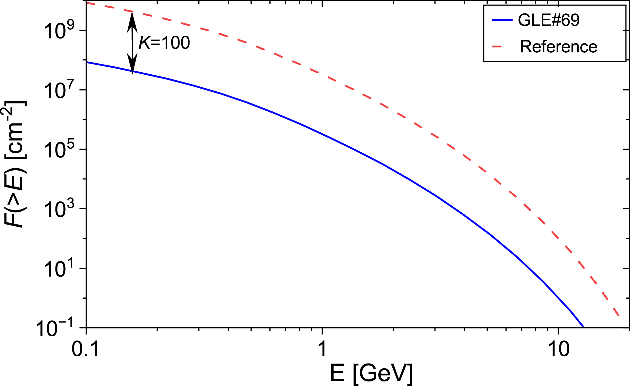
As a reference ESPE energy spectrum for this work, we used that of a recent hard-spectrum Ground Level Enhancement (GLE) #69 (20-Jan-2005), which was well measured by a multitude of ground-based and space-based instruments. That solar particle event was the second largest (≈4500 % instant count rate increase at ground-level polar neutron monitors) and one of the best studied events (e.g., Bieber et al. Reference Bieber, Clem, Evenson, Pyle, Sáiz and Ruffolo2013). Its energy spectrum was shown to correspond to the ESPE spectral characteristics (Koldobskiy et al. Reference Koldobskiy, Mekhaldi, Kovaltsov and Usoskin2023; Mekhaldi et al. Reference Mekhaldi, Adolphi, Herbst and Muscheler2021; Paleari et al. Reference Paleari, Mekhaldi, Adolphi, Christl, Vockenhuber, Gautschi, Beer, Brehm, Erhardt, Synal, Wacker, Wilhelms and Muscheler2022). The spectral shape was taken following a recent full reconstruction (Koldobskiy et al. Reference Koldobskiy, Raukunen, Vainio, Kovaltsov and Usoskin2021), but the intensity was scaled by a freely adjustable scaling factor K, as illustrated in Figure 1. This approach has been validated previously (Golubenko et al. Reference Golubenko, Usoskin, Rozanov and Bard2025). As the reference ESPE, we have considered GLE #69, scaled up by a factor of K = 100 (Figure 1), which roughly corresponds to the sensitivity of the ESPE detection by cosmogenic isotopes (Mekhaldi et al. Reference Mekhaldi, Adolphi, Herbst and Muscheler2021; Usoskin et al. Reference Usoskin, Koldobskiy, Kovaltsov, Rozanov, Sukhodolov, Mishev and Mironova2020). The omnidirectional
Integral omnidirectional fluence of solar energetic particles, F(>E) for the GLE #69 (20-Jan-2005) as reconstructed from ground-based and space-borne data (blue curve—Koldobskiy et al. Reference Koldobskiy, Raukunen, Vainio, Kovaltsov and Usoskin2021). The red dashed curve is scaled up by a factor K=100, representing the reference ESPE spectrum used here.

integral fluence of SEPs with energy above 200 MeV for the reference event is F 200 = 2.78·109 cm−2. We note that the exact spectral shape may only slightly affect the altitude and latitude profile of radiocarbon production, while the total amount of 14C produced by SEPs is defined by the fluence of SEPs with energy above 200 MeV, F 200 (Koldobskiy et al. Reference Koldobskiy, Usoskin and Kovaltsov2022).
The modeling of the Δ14C response was performed by the SOCOL:14C-Ex model (see below) for the Holocene conditions with the CO2 concentration set as 287 ppmv, and the geomagnetic dipole moment M = (9.5 ± 1.0) · 1022 A m2 as corresponding to the end of the preindustrial epoch (Panovska et al. Reference Panovska, Poluianov, Gao, Korte, Mishev, Shprits and Usoskin2023). The total amount of 14C atoms produced by this reference event in the Earth’s atmosphere for this value of M is 3.68·1026, which are produced mostly in the polar stratosphere (Golubenko et al. Reference Golubenko, Rozanov, Kovaltsov and Usoskin2022). This would correspond to an additional global 14C production rate of 2.3 atoms cm−2 s−1, uniformly distributed over one year. This production is superimposed on the normal GCR-related background of about 1.6–2 atoms cm−2 s−1 (Masarik and Beer, Reference Masarik and Beer2009; Poluianov et al. Reference Poluianov, Kovaltsov, Mishev and Usoskin2016), resulting in a total global production rate of about 4 atoms cm−2 s−1 during the event year, i.e., nearly doubling of the annual 14C production.
3D dynamical chemistry—climate model SOCOL:14C-Ex
To model the atmospheric transport of radiocarbon for a very fast and spatially limited 14C production typical for the Miyake events, we use a full dynamical atmospheric chemistry–climate model SOCOL:14C-Ex, specifically adapted for 14C tracing (Golubenko et al. Reference Golubenko, Usoskin, Rozanov and Bard2025; Uusitalo et al. Reference Uusitalo, Golubenko, Arppe, Brehm, Hackman, Hayakawa, Helama, Mizohata, Miyake, Mäkinen, Nöjd, Tanskanen, Tokanai, Rozanov, Wacker, Usoskin and Oinonen2024). The model couples a general circulation model MA-ECHAM (European Centre/HAMburg climate model), with a detailed atmospheric chemistry module, enabling a fully interactive representation of dynamics and chemistry of the low and middle atmosphere. The model’s grid is based on horizontal resolution of 2.8º × 2.8º (spectral truncation T42), corresponding to 128 longitude and 64 latitude grid points. The vertical domain comprises 39 hybrid σ–pressure levels, extending from the surface to about 80 km altitude (0.01 hPa), covering the troposphere, stratosphere, and mesosphere.
SOCOL:14C-Ex is a chemistry-climate model of the SOCOL family, built on SOCOLv3 (SOlar Climate Ozone Links, version 3—Stenke et al. Reference Stenke, Schraner, Rozanov, Egorova, Luo and Peter2013) with the AER aerosol microphysics module (Sheng et al. Reference Sheng, Weisenstein, Luo, Rozanov, Stenke, Anet and Peter2015; Weisenstein et al. Reference Weisenstein, Yue, Ko, Sze, Rodriguez and Scott1997), the MA–ECHAM5 atmospheric dynamics core (Hommel et al. Reference Hommel, Timmreck and Graf2011), and the MEZON chemistry module (Egorova et al. Reference Egorova, Rozanov, Zubov and Karol2003). Aerosol processes and atmospheric chemistry are interactively coupled with circulation, with information exchange between modules every two model hours. For 14C transport, the isotope is treated as a passive gaseous tracer subject to source and sink terms.
The production of 14C is calculated using the CRAC:14C production model (Poluianov et al. Reference Poluianov, Kovaltsov, Mishev and Usoskin2016) for SEPs. Radiocarbon produced by galactic cosmic rays (GCRs) is assumed to be a constant background upon which the SEP-related 14C is added, because the 11-yr solar-cycle related variability in Δ14C is small (about 2‰—e.g., Brehm et al. Reference Brehm, Bayliss, Christl, Synal, Adolphi, Beer, Kromer, Muscheler, Solanki, Usoskin, Bleicher, Bollhalder, Tyers and Wacker2021), and its phase is unknown for ancient periods.
Climatic boundary conditions, such as sea surface temperature, sea-ice cover, and atmospheric CO2 concentration (Marcott et al. Reference Marcott, Bauska, Buizert, Steig, Rosen, Cuffey and Brook2014), are chosen to match the exact epoch for the event under consideration (e.g., Late Glacial), and are consistently simulated within the SOCOL framework. For the analyzed events, full simulations were conducted under realistic atmospheric conditions. Each simulation run consisted of six years of spin-up followed by seven years of post-event simulation.
The carbon sink scheme is simplified to include only biospheric uptake and exchange with surface ocean waters, parameterised according to surface albedo, seasonality, and land–ocean distribution (Golubenko et al. Reference Golubenko, Usoskin, Rozanov and Bard2025). Ice-covered surfaces (albedo ≥ 0.7) are considered inert. Oceanic sinks operate year-round in ice-free regions with an exchange time of 8.29 years (Güttler et al. Reference Güttler, Adolphi, Beer, Bleicher, Boswijk, Christl, Hogg, Palmer, Vockenhuber, Wacker and Wunder2015). Terrestrial sinks operate during the vegetation growth season according to the Leaf Area Index (LAI—Verger et al. Reference Verger, Sánchez-Zapero, Weiss, Descals, Camacho, Lacaze and Baret2023), defined as (i) year-round in the tropics, (ii) six months centred on the summer solstice in mid-latitudes, and (iii) absent beyond the polar circles.
Return flux from the surface ocean to the atmosphere is neglected during the short time window considered. This modeling approach assumes a steady-state carbon cycle, including the oceanic reservoirs, and is designed to isolate the effect of a hypothesized extra source of very young carbon on the atmospheric Δ14C peak. While recent carbon-cycle studies show that the oceanic feedback can influence atmospheric carbon on decadal timescales (e.g., Miller et al. Reference Miller, Lehman and Lindsay2025), transient simulations show that even strong perturbations of ocean circulation translate into relatively modest atmospheric Δ14C changes over the first decades. As underlined by Bard et al. Reference Bard, Miramont, Capano, Guibal, Marschal, Rostek, Tuna, Fagault and Heaton2023, steady-state estimates based on multi-box models suggest that halving the meridional overturning circulation could increase atmospheric Δ14C by 35–40‰ (Bard et al. Reference Bard, Raisbeck, Yiou and Jouzel1997), whereas transient simulations over a century yield only about an 8‰ increase (Goslar et al. Reference Goslar1995; Hughen et al. Reference Hughen, Overpeck, Lehman, Kashgarian, Southon, Peterson, Alley and Sigman1998). Transients of similar magnitude were obtained with more sophisticated 2D-3D carbon cycle models (Delaygue et al. Reference Delaygue, Stocker, Joos and Plattner2003; Singarayer et al. Reference Singarayer, Richards, Ridgwell, Valdes, Austin and Beck2008). Therefore, oceanic feedbacks alone are too slow to explain the magnitude and abruptness of the observed Δ14C peak, and neglecting oceanic return fluxes is justified within the limited temporal scope of the present study. Furthermore, the main problem is that in order to explain even part of the atmospheric Δ14C peak requires an extra source of very young carbon, which is incompatible with oceanic or terrestrial sources (e.g. permafrost).
The resulting uncertainty (up to 2‰ in Δ14C—see Golubenko et al. Reference Golubenko, Usoskin, Rozanov and Bard2025) is taken into account in model-data fitting. Long-term decay and deep-ocean overturning of 14C are not simulated, as their influence on short-term post-event dynamics is negligible.
For robustness, each scenario was simulated as an ensemble of three independent runs with identical boundary conditions. The inter-run variability was found to be very small (below 1% in 14C concentration, corresponding to < 0.4‰ in Δ14C peak amplitude), and therefore only a single median representative realisation is presented for each event.
In SOCOL:14C-Ex, the simulated output for the near-surface atmosphere is the absolute concentration of 14C, denoted henceforth as C, expressed in 14C atoms per cubic meter of air (atoms/m3). For comparison with observational Δ14C datasets, these values are transformed into per mil (‰) units (Stuiver and Polach Reference Stuiver and Polach1977): ${\Delta ^{14}}{\rm{C}} = \left( {{{{A_{\rm{S}}}} \over {{A_{{\rm{abs}}}}}} - 1} \right) \cdot 1000,$
where A abs = 226 Bq/kgC and A S denotes the specific activity of radiocarbon in near-surface air. Assuming the standard air density at sea level, ρ = 1236 g m−3, this corresponds to d = 0.123 grams of carbon per cubic meter of air. The number of 14C atoms per kilogram of carbon is then obtained as C/d. The computed concentration can be converted to activity using the mean lifetime of 14C, τ = 2.62 · 1011 s as ${A_{\rm{S}}} = {C \over {d\tau }}[{\rm{Bq/kgC}}].$
Finally, the concentration can be directly converted into the corresponding Δ14C value as ${\Delta ^{14}}{\rm{C}} = 3.305 \cdot {10^{ - 5}} \times {C \over \nu },$
where ν is CO2 concentration (in ppmv) for the period of interest.
Modeled Δ14C response to an ESPE
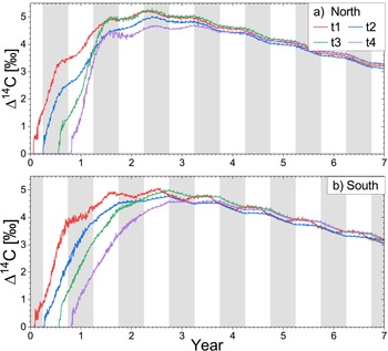
The modeled daily Δ14C response to the reference ESPE is exemplified in Figure 2 for four dates of the event occurrence: 20-Jan, 01-Apr, 20-Jul, and 20-Oct, denoted as t1– t4, respectively. The responses are shown for the end of the preindustrial era (zero time corresponds to 01-Jan-1865, CO2 concentration ν = 287 ppmv), for two nearly antipodal locations: Central Europe (44.31ºN, 5.52ºE), and Patagonia (41.9ºS, 72.67ºW). For the computations, the production was modeled as a δ-function (instant production). In case of prolonged production, e.g., a series of events separated by days–months, as produced by a long-living solar active region, a superposition of response functions can be used.
Examples of the time response functions of Δ14C to the reference ESPE (Figure 1) for two geographical locations: Central Europe (44.31ºN, 5.52ºE—panel a), and Patagonia (41.9ºS, 72.67ºW—panel b). Different curves correspond to different dates of the ESPE occurrence, as indicated in the legend: 20-Jan, 01-Apr, 20-Jul, and 20-Oct of year zero (1865 in the simulation), denoted as t1–t4, respectively. Shaded areas approximately indicate the tree growth periods. The results are shown with daily resolution, depicting, in particular, meteorological noise on the synoptic scale.

The modeled Δ14C profiles depict a weak annual cycle caused by the stratosphere-troposphere exchange in the spring season, and the seasonality of the carbon sinks. The more pronounced annual cycle in the Southern Hemisphere reflects the stronger and more stable Antarctic polar vortex compared to the Northern Hemisphere. Such a strong vortex retains the isotopic signal longer at high latitudes and leads to sharper “pulsations” in the exchange with lower latitudes. In the Northern Hemisphere, the circulation is more ragged, due to frequent stratospheric sudden warmings (SSWs) and vortex breakdowns, leading to better smoothing of the annual cycle in Δ14C. It can also be seen that the response is slightly weaker in the Southern Hemisphere, because of the larger sink area in the ocean.
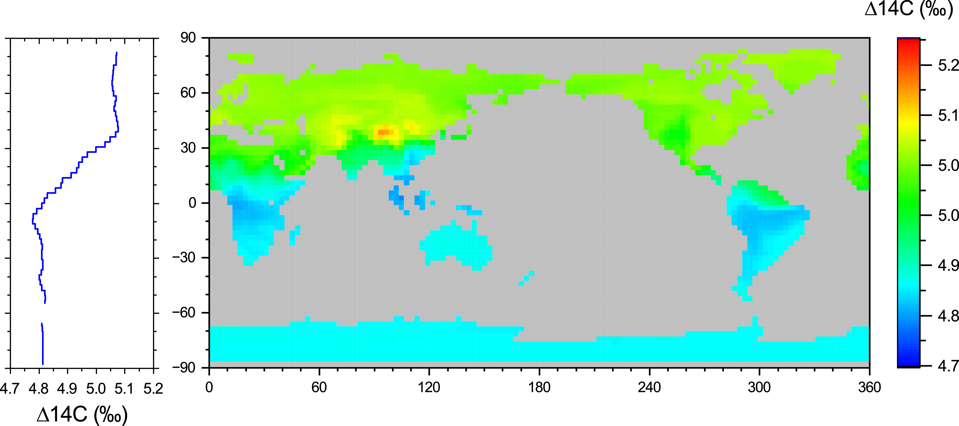
The above curves were shown for the prescribed geographical locations, but the model results are defined for all locations on Earth. As an example, Figure 3 shows a snapshot of the modeled Δ14C geographical distribution over land for the day of 20-Jul-1867, viz. 2.5 years after the reference event occurred on 20-Jan-1865. The distribution appears uneven, with several distinct features. First, there is a significant hemispheric difference with the Δ14C signal being 0.2–0.3‰ higher in the Northern Hemisphere. This is partly related to the fact that mid-July is mid-boreal-summer, after the stratosphere-troposphere exchange event, which brings radiocarbon from the stratosphere down to the surface level. On the contrary, the polar stratospheric radiocarbon is blocked by the polar vortex in the Southern Hemisphere. This pattern may change during the boreal winter. Another interesting feature is the tropical dip in Δ14C, which is caused by the ascending flow of the Brewer-Dobson circulation. The third feature is regional and observed as a slightly enhanced Δ14C signal in the Himalaya and Gobi desert region, caused by the high altitude and the absence of a carbon sink. Such features cannot be modeled by a standard box model and require full dynamic modeling.
Geographical distribution of modeled near-ground overland Δ14C values caused by the reference ESPE, which took place on 20-Jan-1865. The distribution is shown for the day of 20-Jul-1867. The LHS panel depicts the latitudinal zonal (over land) mean.Panel A: A line graph depicting the latitudinal zonal mean over land. The x-axis represents delta 14C values ranging from 4.7 to 5.2 percent, and the y-axis represents latitude ranging from –90 to 90 degrees. The line graph shows a trend with variations in delta 14C values across different latitudes. Panel B: A heat map showing the geographical distribution of modeled near-ground overland delta 14C values. The x-axis represents longitude ranging from 0 to 360 degrees, and the y-axis represents latitude ranging from –90 to 90 degrees. The color scale on the right indicates delta 14C values ranging from 4.7 to 5.2 percent. Higher values are associated with lighter colors, and lower values are associated with darker colors. The heat map shows a concentration of higher delta 14C values in certain regions, particularly in the northern hemisphere.

The modeled Δ14C response curves are provided with daily resolution, but they need to be compared to the annual Δ14C data measured in tree rings. Accordingly, we have computed annual Δ14C values averaged over the local tree growth period, separately for Northern and Southern Hemispheres as illustrated by shaded stripes in Figure 2. The averaging was done individually for each location (see Golubenko et al. Reference Golubenko, Usoskin, Rozanov and Bard2025 for details). This accounting for the tree growing season is crucially important to define the timing of the production event as discussed later.
A set of the response time profiles
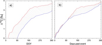
Only four response curves, corresponding to different seasons, were computed with the full SOCOL model simulation for each hemisphere (Figure 2). Doing it with a higher cadence would be unfeasible because of the large computational time of ≈10 wall-clock days for each curve. To produce daily response curves, we linearly interpolated between the fully computed curves as illustrated in Figure 4, assuming that the difference on the short timescale is gradual. First, the modeled curves were slightly smoothed with a 27-day low-pass filter to remove the meteorological noise—see red and blue curves in Figure 4a. Next, the smoothed modeled curves were joined in time to start on the event day, as shown in Figure 4b (the event day is day 0). Then the daily response curves were calculated as a linear interpolation between the nearest fully modeled ones, as shown by gray curves in panel b (every tenth gray curve is shown).
An example of interpolating the response curves for the first year of the ESPE. Panel a: full-model calculated responses for 20-Jan (red) and 01-Apr (blue) in the Northern Hemisphere—similar to Figure 2, along with interpolated curves (gray) shown for every tenth day. Panel b: Similar to panel a, but all the curves start on the event’s date.

Finally, the interpolated curves were detouched again to start on the exact event day, as shown by the gray curves in panel a. These response curves with a daily cadence were further used in the data fitting, as described below.
Interesting in Figure 4b is that the modeled curves for the 20-Jan and 01-Apr event occurrence dates coincide for the first hundred days and then start diverging. This can be interpreted so that the first Δ14C response is to radiocarbon produced in the troposphere, with its fast transport for all seasons, on the one hand. On the other hand, the vertical transport, which brings the stratospheric radiocarbon down, differs between seasons and makes the red curve rise faster due to the fast stratosphere-troposphere exchange in midSpring.
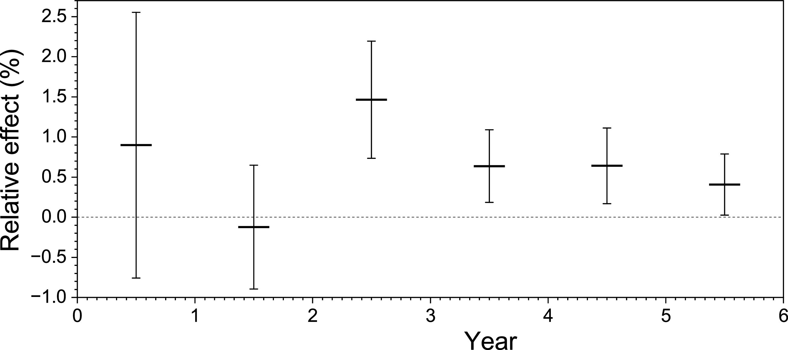
The model computations were focused on the Holocene period, but one of the analyzed events, of 12,351 BC, took place during the late Glacial period. This may affect our analysis in two ways, via the atmospheric transport and the carbon sinks, which could be different during the Glacial. The former difference was shown to be negligibly small (Golubenko et al. Reference Golubenko, Usoskin, Rozanov and Bard2025). The carbon sink to the ocean is modeled, explicitly considering the ice cover, and thus is adaptive to climate change. The sink of carbon to the biosphere might be overestimated by the model, since the model considers the Holocene-type vegetation pattern, while vegetation was suppressed during the Glacial (Jeltsch-Thömmes et al. Reference Jeltsch-Thömmes, Battaglia, Cartapanis, Jaccard and Joos2019; Prentice and Fung Reference Prentice and Fung1990). To evaluate this effect, we performed a modeling of the response curve for T = 20 DoY, switching off the biospheric sink in the regions identified as extreme deserts (Adams and Faure Reference Adams and Faure1998). The percentile difference between the reference event’s amplitude as reconstructed for model runs with and without considering the Glacial-type biosphere is shown in Figure 5. As seen, the effect is consistent with zero for the first two years, when the produced radiocarbon remains largely in the atmosphere, but the difference becomes systematically positive yet formally insignificant from year 3 onward, owing to the reduced biospheric sink. The effect is negligibly small, about 0.7% of the production signal, which translates, for the event of 12,351 BC, to ≈ 0.3‰. This exercise can serve as a conservative upper limit for the reduced biosphere’s effect. Accordingly, we neglected this effect in further analysis. The reference Δ14C response time profiles are presented in Appendix B.
Estimated effect of including a Glacial-type biosphere in the model. The plot shows the percentile difference between the near-ground air 14C concentrations in Southern Europe, averaged over April–September for years following a reference ESPE occurring at the zero date. The concentrations were computed by the SOCOL:14C-Ex model runs for the Glacial and Holocene vegetation types. The difference is shown as Glacial minus Holocene conditions. The error bars represent the statistical uncertainties between model runs.

Data analysis
Here, we demonstrate the ability of the new dynamical SOCOL:14C-Ex model to analyze the Miyake event and estimate the parameters of the parent ESPEs, including an assessment of the full uncertainties.
Miyake events analyzed here
We applied the model and methodology described above to analyze seven Miyake events recorded in radiocarbon for the past 14 millennia, from the Late Pleistocene (12,351 BC) to the first millennium AD, as summarized below and in Table 1. We collected available high-resolution data of Δ14C for these events from the literature. All records are based on annually resolved tree-ring chronologies, some offering earlywood/latewood separation or sub-annual precision. In such cases, early and late-wood data were subjected to a weighted average to produce annual data. We did not use the data with a temporal resolution > 1 year. An inventory of the used datasets and their sources is provided in Appendix A. When dating the event, we use the ESPE year as derived from our analysis, although the onset of the 14C response can be delayed by about one year (e.g., for AD 774/775). The historical date convention (no year zero) is used.
-
• 12,351 BC (14,300 BP) during late glacial period, transition to Holocene: The highest known ∼40‰ rise in Δ14C detected in sub-fossil Scots pines from the Italian and French Alps, during deglaciation (Bard et al. Reference Bard, Miramont, Capano, Guibal, Marschal, Rostek, Tuna, Fagault and Heaton2023).
-
• 7177 BC (9126 BP), Early Holocene, post-Younger Dryas: One of the strongest radiocarbon anomalies (∼15‰) over the Holocene, observed in several high-resolution datasets in the Northern hemisphere (Brehm et al. Reference Brehm, Christl, Knowles, Casanova, Evershed, Adolphi, Muscheler, Synal, Mekhaldi, Paleari, Leuschner, Bayliss, Nicolussi, Pichler, Schlüchter, Pearson, Salzer, Fonti, Nievergelt and Wacker2022).
-
• 5411 BC (7360 BP), Holocene climate optimum: A strong radiocarbon enhancement (∼8‰) observed in several high-resolution datasets from the Northern hemisphere (Miyake et al. Reference Miyake, Panyushkina, Jull, Adolphi, Brehm, Helama, Kanzawa, Moriya, Muscheler, Nicolussi, Oinonen, Salzer, Takeyama, Tokanai and Wacker2021).
-
• 5260 BC (7209 BP), Holocene climate optimum: One of the strongest Holocene ra-diocarbon anomalies (∼20‰), observed in several high-resolution datasets from the Northern hemisphere (Brehm et al. Reference Brehm, Christl, Knowles, Casanova, Evershed, Adolphi, Muscheler, Synal, Mekhaldi, Paleari, Leuschner, Bayliss, Nicolussi, Pichler, Schlüchter, Pearson, Salzer, Fonti, Nievergelt and Wacker2022).
-
• 664 BC (2613 BP), late Holocene: A strong ∼10‰ radiocarbon enhancement recorded in several Northern Hemisphere trees (Panyushkina et al. Reference Panyushkina, Jull and Molnár2024; Park et al. Reference Park, Southon, Fahrni, Creasman and Mewaldt2017; Rakowski et al. Reference Rakowski, Krąpiec, Huels, Pawlyta, Hamann and Wiktorowski2019; Sakurai et al. Reference Sakurai, Tokanai, Miyake, Horiuchi, Masuda, Miyahara, Ohyama, Sakamoto, Mitsutani and Moriya2020).
-
• AD 774 (1176 BP), Early Medieval period: One of the strongest radiocarbon anomalies (∼18‰), observed in several high-resolution datasets in the Northern hemisphere and Southern hemispheres. This is the best-studied ESPE (Büntgen et al. Reference Büntgen, Wacker, Galván, Arnold, Arseneault, Baillie, Beer, Bernabei, Bleicher, Boswijk, Bräuning, Carrer, Ljungqvist, Cherubini, Christl, Christie, Clark, Cook, D’Arrigo and Young2018; Güttler et al. Reference Güttler, Adolphi, Beer, Bleicher, Boswijk, Christl, Hogg, Palmer, Vockenhuber, Wacker and Wunder2015; Jull et al. Reference Jull, Panyushkina, Lange, Kukarskih, Myglan, Clark, Salzer, Burr and Leavitt2014; Miyake et al. Reference Miyake, Nagaya, Masuda and Nakamura2012; Park et al. Reference Park, Southon, Fahrni, Creasman and Mewaldt2017; Scifo et al. Reference Scifo, Kuitems and Neocleous2019; Usoskin et al. Reference Usoskin, Kromer, Ludlow, Beer, Friedrich, Kovaltsov, Solanki and Wacker2013; Walker et al. Reference Walker, Shobe, Andrea-Hayles, Dey, Suran, Baatarbileg and Hessl2025).
-
• AD 993 (957 BP), Early Medieval period: A strong ∼10‰ radiocarbon enhancement recorded in several trees in both Northern and Southern Hemispheres (Büntgen et al. Reference Büntgen, Wacker, Galván, Arnold, Arseneault, Baillie, Beer, Bernabei, Bleicher, Boswijk, Bräuning, Carrer, Ljungqvist, Cherubini, Christl, Christie, Clark, Cook, D’Arrigo and Young2018; Miyake et al. Reference Miyake, Masuda and Nakamura2013).
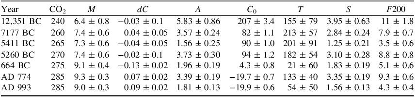
Summary of the analyzed Miyake events and ESPEs: year of the ESPE event; atmospheric CO2 concentrations in ppmv (Indermühle et al. Reference Indermühle, Stocker, Joos, Fischer, Smith, Wahlen, Deck, Mastroianni, Tschumi, Blunier, Meyer and Stauffer1999; Marcott et al. Reference Marcott, Bauska, Buizert, Steig, Rosen, Cuffey and Brook2014); VDM M in 1022 A m2 (Panovska et al. Reference Panovska, Poluianov, Gao, Korte, Mishev, Shprits and Usoskin2023); Δ14C trend dC in ‰ year−1; scaling of the reference response A (see Table 2); background level C0 in ‰ (Table 2); Estimated date of the event T in DoY (Table 2); ESPE strength S (Equation 6); and the estimated fluence of SEPs with energy >200 MeV F200 in 109 cm−2.

Data fitting
First, data from the modeled daily Δ14C curves were averaged over the tree/growth season for each location to represent the annual Δ14C values measured in tree rings as illustrated in Figure 2, similar to Golubenko et al. (Reference Golubenko, Usoskin, Rozanov and Bard2025). Thus computed annual modeled Δ14C were compared with the measured data by fitting the annual model curves into the measured data sets and finding the optimal parameters as described below. The parameters to be determined were: the start date of the event T, quantified as the day of year (DoY) of the prescribed year (negative DoY refers to the previous year), leap years were neglected (all years are assumed to have 365 days); the pre-increase level C 0 in ‰, which quantifies the background Δ14C level due to GCR; and the amplitude of the event in units of the reference ESPE, A. $D^* = A\cdot\mathcal{D}^\dagger(T) + C_0,$
where D* denote the measured Δ14C values to be fitted, and D†(T) is the modeled response to the reference ESPE, which occurred on day T. The parameters T and A were fitted simultaneously for all datasets for the whole event, while C 0 was found individually for each hemisphere. For each event, we fitted nine annual data points: two for the pre-event years assuming no ESPE signal in the model data, and seven annual points of the event. If some measured values were missing in a dataset, fewer data points were used in the fit, respectively.
Sometimes Miyake events occur in the background of changing Δ14C level due to the global carbon cycle, as, e.g., for the event of 664 BC (Usoskin et al. Reference Usoskin, Chatzistergos, Solanki, Krivova, Kovaltsov, Brehm, Christl and Wacker2025). The trend may distort the fitting and needs to be corrected for. We have evaluated the linear trend dC in Δ14C around the events as follows: the measured Δ14C data for 20 years before the event start date and years 20–40 past the event were fitted by a linear trend considering data uncertainties. The data were used as: annual for the past three millennia (Brehm et al. Reference Brehm, Bayliss, Christl, Synal, Adolphi, Beer, Kromer, Muscheler, Solanki, Usoskin, Bleicher, Bollhalder, Tyers and Wacker2021, Reference Brehm, Pearson, Christl, Bayliss, Nicolussi, Pichler, Brown and Wacker2025; Fahrni et al. Reference Fahrni, Southon, Fuller, Park, Friedrich, Muscheler, Wacker and Taylor2020), and 5-year before that (IntCal20—Reimer et al. Reference Reimer, Austin, Bard, Bayliss, Blackwell, Ramsey, Butzin, Cheng, Edwards, Friedrich, Grootes, Guilderson, Hajdas, Heaton, Hogg, Hughen, Kromer, Manning, Muscheler and Talamo2020). The obtained trend values are shown in Table 1, As seen, the events of 664 BC, AD 774 and AD 993 depict a weak but significant trend, while the trend is consistent with zero for other events. For the fitting, the data were detrended using the dC values from Table 1.
To assess the robustness of the procedure, the fits were performed by applying two different approaches—the fitting based on χ 2 statistics, and the MCMC (Markov Chain Monte Carlo) approach, as described below.
Statistical χ2 method
The statistical approach is based on the χ 2-statistics. The modeled curves are assumed to be error-free, with the uncertainties being related to the measured data. As the merit function for the fit, we considered the χ 2 value defined as ${\chi ^2} = \sum\limits_i^N {{{\sum\limits_{j = 1}^{{k_i}} {\left( {{{D_j^* - {D_{i,j}}} \over {{\sigma _{i,j}}}}} \right)} }^2},} $
where D
i,j
and σ
i,j
are the values of Δ14C measured in i-th dataset for j-th year along with their 1σ error bars, respectively; $D_j^*(T)$
are the corresponding modeled Δ14C values for the jth year, defined by Equation 4, and k
i
is the number of meaningful annual points in the i-th dataset (k=9 if there are no missing data points). The modeled curves D† and the pre-increase level C
0 were considered separately for the Northern and Southern Hemispheres, while the values of A and T were the same for each event over the entire globe.
$D_j^*(T)$
are the corresponding modeled Δ14C values for the jth year, defined by Equation 4, and k
i
is the number of meaningful annual points in the i-th dataset (k=9 if there are no missing data points). The modeled curves D† and the pre-increase level C
0 were considered separately for the Northern and Southern Hemispheres, while the values of A and T were the same for each event over the entire globe.
The parameter values were scanned in a reasonable range, and a set of parameter values, minimising the value of χ
2, viz. χ
2
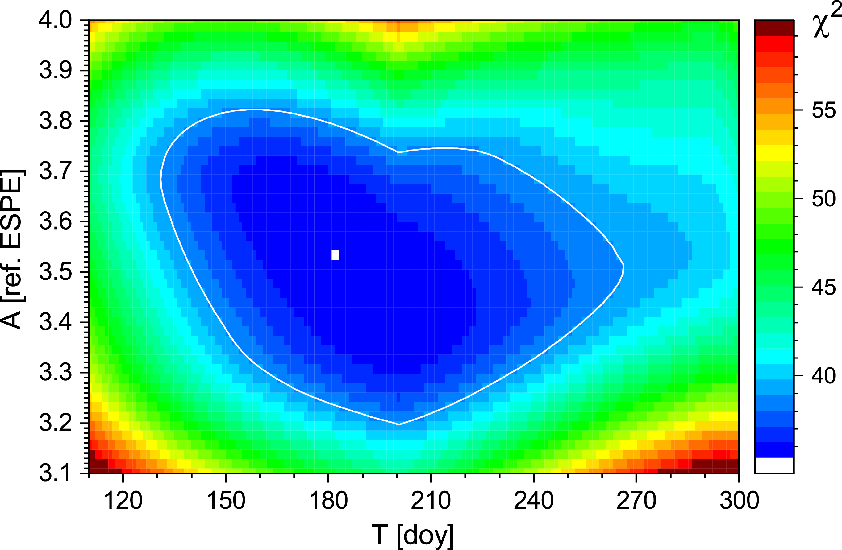
min, was set for each studied event. The 68% confidence intervals of the parameters were defined as bounded by the condition of ${\chi ^2} \le \chi _{\min }^2 + 3.53$
for three independent parameters, viz. A, C
0 and T. An example is shown in Figure 7, and the best-fit values and the results are summarized in Table 2.
${\chi ^2} \le \chi _{\min }^2 + 3.53$
for three independent parameters, viz. A, C
0 and T. An example is shown in Figure 7, and the best-fit values and the results are summarized in Table 2.
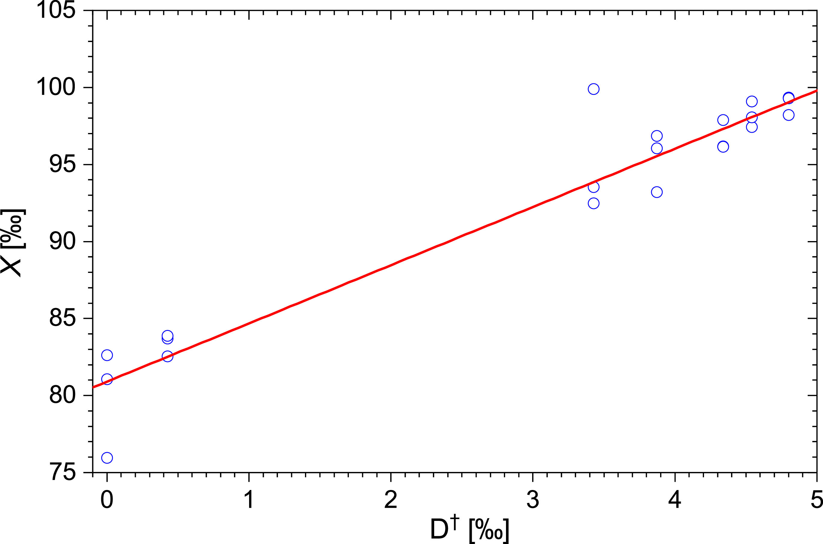
Example of the MCMC determination of the best-fit parameters for the event of 7177 BC (9126 BP). Blue dots depict annual values X for one random realisation of three datasets (Y-axis) vs. the reference model curve D† for T=207 doy. The red line is the linear regression Xi,j = 3.78 · Dj † + 80.9.

Example of the determination of the best-fit parameters, T (in DoY of 7177 BC [9126 BP]) and scaling factor A for the ESPE of 7177 BC (9126 BP). The colour code represents the value of χ2 (Equation 5). The best-fit set of parameters (A=3.54, T=183), corresponding to the minimal value of χ2 min=35.4, is depicted by the white dot, while the white line bounds the 68% confidence areas (χ2 = χ2 min + 3.53).

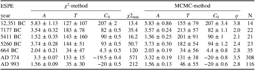
Best-fit parameters, viz. A, T [DoY], and C0 [‰], along with their 68% confidence intervals, for the seven ESPEs, analyzed here, by two methods—χ2 and MCMC. Shown are also the values of the merit functions χ2 min and RMSE ǫ. The last column depicts the number of the fitted datapoints N.

MCMC approach
The MCMC approach is not based on any specific statistics, but includes all possible uncertainties straightforwardly via randomisation of the datasets. This was done in the following way.
-
1. First, a randomised dataset X i,j = D i,j + Rn · σ i,j is produced, where D i,j and σ i,j are the measured values of Δ14C in the i-th dataset for the j-th year along with their uncertainties, and R n are normally distributed random numbers with zero mean and unit dispersion.
-
2. The hypothetical date of the event T is selected that determines the selection of the fitting curves D j †, which were considered separately for the two hemispheres. The randomised dataset X is fit linearly by the fitting curve D *(T) as illustrated in Figure 6. The best-fit values of C 0 and A are found by the least-squares method. The RMSE (root mean squared error) value ǫ was calculated for the fitting.
-
3. Step 2 is repeated 365 times by scanning, with a daily cadence, over T for one year around the guessed event date. The scan can be extended if needed. The set of C 0 ′, A ′, and T ′ providing the absolute minimum of RMSE is fixed.
-
4. Steps 1–3 are repeated N = 10000 times, each time using a new set of X based on a random-number set R n . This yields a distribution of the parameter values C 0 ′, A ′, and T ′. From these distributions, the mean values and the standard deviations can be computed as the estimates for the reconstructed ESPE strength (the value of A) and timing T, as illustrated in Figure 8.
Figure 8.Distribution density of 3000 points in the A-vs-T parameter space, for the MCMC analysis of the event of 7177 BC (9126 BP). Each point corresponds to one realisation similar to that shown in Figure 6. Distributions of the values of T and A are shown on the panels on the top and on the right, respectively. The black circle denotes the gravity centre of the distribution (A=3.57 and T=213).


An example of an analysis for 7177 BC (9126 BP)
The analysis is illustrated here for the ESPE of 7177 BC (see Table 2). First, we performed the χ 2 analysis as shown in Figure 7, which depicts the dependence of χ 2 on the values of T and A (C 0 is fixed at 82 ‰ for the plot). The minimum value of χ 2 min is 35.4 (the number of degrees of freedom is 22), corresponding to A = 3.76 and T = 183 DoY (white spot in the Figure). We note that the best fit yields 1.6 χ 2 per degree of freedom, suggesting that the spread of experimental points is broader than defined solely by the formal error bars, or that the used model may be not perfect. The increment of χ 2 min by 3.53 bounds the 68% confidence area, as shown by the white line in the Figure. The best-fit parameters of the ESPE of 7177 BC were found (see Table 2) as A = 3.54 ± 0.32, T = 183 ± 78 days, and C0 = 82 ± 0.5‰.
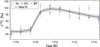
An example of the model curve fit by the MCMC method for the same event is shown in Figure 8. The central panel depicts the distribution density of the best-fit parameter sets of A and T (values of C 0 are not shown). Distributions of the individual parameter values are shown in the side panels along with the best-fit normal distributions, from which the mean and the standard deviation were obtained for each parameter. The best-fit parameter set corresponds to the gravity centre of the distribution as denoted by the black dot in the central panel. The 68% confidence intervals of the parameter values are defined from the normal distributions (side panels) as ± 0.26 and ± 57 for A and T, respectively, as entered in Table 2. The RMSE value of the fit is ǫ ≈ 2‰, which is comparable to the measurement errors. The fit is illustrated in Figure 9.
Illustration of fitting of the measured Δ14C datasets (points) for the ESPE of 7177 BC (9126 BP) with the model curves using the MCMC method. The datasets are from Brehm et al. Reference Brehm, Bayliss, Christl, Synal, Adolphi, Beer, Kromer, Muscheler, Solanki, Usoskin, Bleicher, Bollhalder, Tyers and Wacker2021: Alpine Larch (AL), German Oak (GO), and Bristlecone Pine (BP)—see Table 1. The best fit with 1σ model uncertainties (see Table 2) is depicted by the solid black line with gray shading.

It is important that both χ 2 and MCMC methods, which are totally independent of each other and based on different types of statistics and merit functions, produce very similar results. All best-fit parameter values in Table 2 are close to each other and fully consistent within the 68% confidence intervals. For further analysis, we use the results produced by the MCMC method, which is more robust and stable with respect to the measurement error estimates.
The analysis was performed in the same way for all analyzed events, with the results summarized in Table 2.
Estimate of extreme solar events
The estimated dates of the events are distributed broadly between winter and late summer for the best-fit values and cover the entire year within the uncertainties. We have checked with the Kolmogorov-Smirnov test that the distribution of the event dates over the year is consistent with the uniform distribution at the p−value <0.01. This suggests that no artificial seasonal bias has been introduced in the analysis.
The strength of the Δ14C responses to the reference event was estimated for the known Miyake events (Table 2). However, the amount of the produced radiocarbon and, thus, the response of Δ14C for the same ESPE may be different, as defined by the conditions during the time of the event: geomagnetic field strength, quantified via the geomagnetic virtual dipole moment (VDM) M; the content of CO2 in the atmosphere ν; and potentially the type of climate. The climate dependence was shown to be negligibly small, within 1% of the response, i.e. <0.4‰ even for the strongest event (Golubenko et al. Reference Golubenko, Usoskin, Rozanov and Bard2025). The other two effects cannot be neglected and must be properly accounted for to relate the strength of the Miyake events in Δ14C to the strength of he corresponding ESPE.
The correction for the CO2 level ν is a simple linear scaling, as defined by Equation 3. The higher the CO2 concentration ν is, the smaller is the Δ14C response to the same ESPE. Correction for the geomagnetic field strength is not linear, but also straightforward (see Figure 5 in Golubenko et al. Reference Golubenko, Usoskin, Rozanov and Bard2025): the Δ14C response is scaled with the VDM value M as M −0.55, viz., the stronger the geomagnetic field is, the smaller is the Δ14C response to the same ESPE. The adopted values of the VDM and ν are listed in Table 1 for the analyzed events.
Since the paleomagnetic models are not precise and include uncertainties in the VDM reconstructions, they were included via the MCMC error-propagation approach, into the uncertainties of the final ESPE strength estimates S: $S = A\cdot{\left( {{M \over {{M_0}}}} \right)^{0.55}}\cdot{\nu \over {{\nu _0}}},$
where M 0 = 9.5 · 1022 A m2 and ν 0 = 287 ppmv correspond to the VDM and CO2 concentration for which the reference response was computed.
The reconstructed strengths of ESPEs, S, along with their 68% confidence intervals, are listed in the right-hand-side block of Table 1, as well as the corresponding F 200 fluences of SEPs. As seen, the correction for geomagnetic and CO2 factors modifies the ranking of the events significantly. For example, the 12,351 BC (14,300 BP) Miyake event was about 72% higher than that of AD 774, but the corresponding ESPE was only 18% stronger, in full agreement with the results by Golubenko et al. (Reference Golubenko, Usoskin, Rozanov and Bard2025). This is explained by two factors, both enhancing the Δ14C response, viz. weaker geomagnetic field and a smaller CO2 concentration (Table 1)—see Golubenko et al. (Reference Golubenko, Usoskin, Rozanov and Bard2025) for more details. While the Miyake event of AD 774 was only the third highest for the Holocene, the corresponding ESPE was found, after the correction, to be the strongest one over the Holocene and the second strongest in the entire record. We note that the F 200 fluence for each ESPE is at least an order of magnitude stronger than the total F 200 fluence of SEPs, 0.5·109 cm−2, registered over the last three full solar cycles 1984–2020 (Raukunen et al. Reference Raukunen, Usoskin, Koldobskiy, Kovaltsov and Vainio2022).
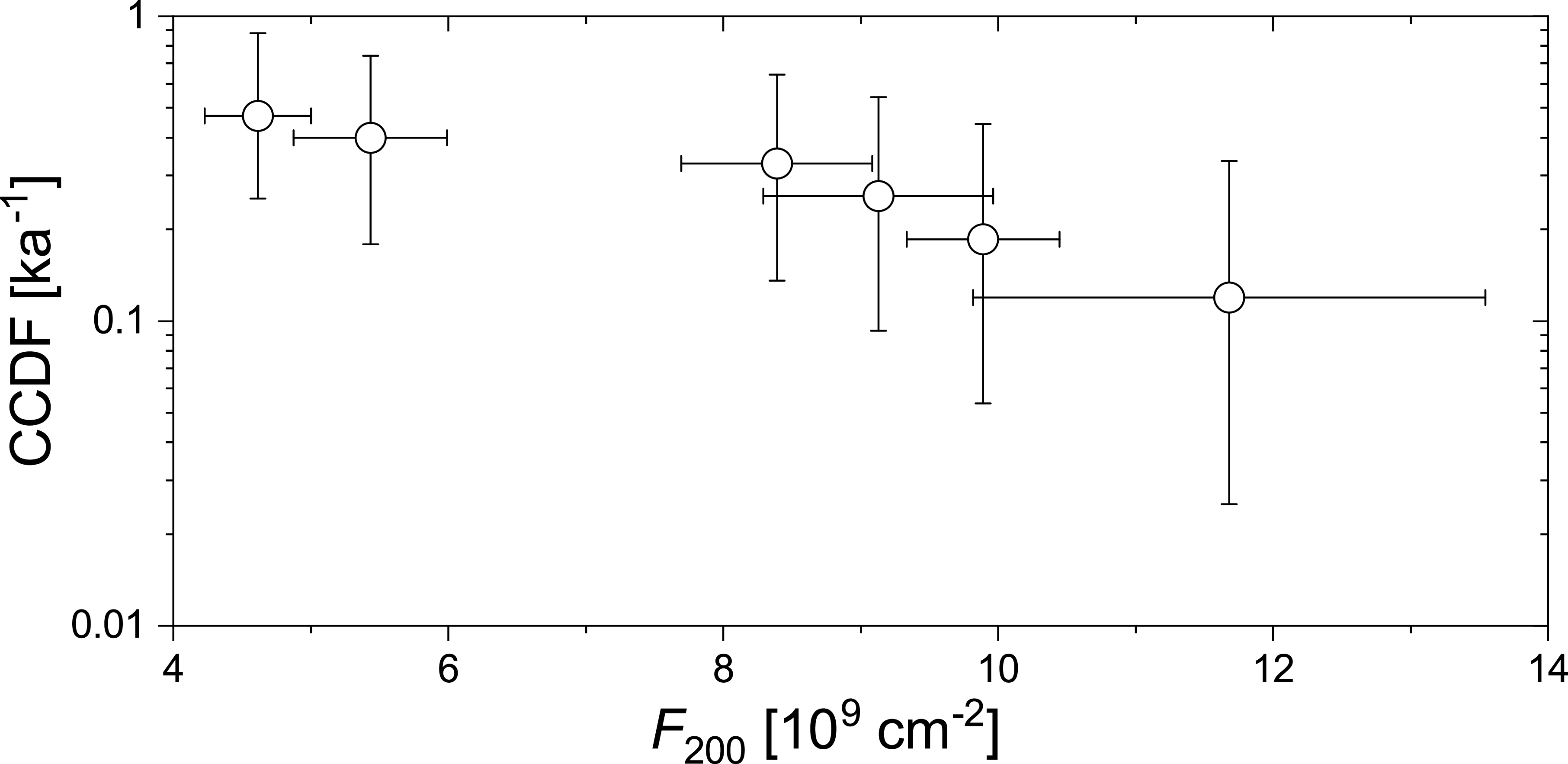
Figure 10 depicts the complementary cumulative distribution function (CCDF) of the occurrence, within a millennium, of an ESPE with the F 200 fluence of SEP exceeding the given F 200 value. The CCDF is computed using confirmed and published events listed in Table 1. We assumed that all events are independent of each other and thus applied the Poisson statistics to evaluate the CCDF. The occurrence probability of a clearly detectable ESPE is roughly once in two millennia (68% confidence interval covers the range from once in three millennia to once per millennium). The strongest ESPE of 12,351 BC (14,300 BP) has the occurrence probability of roughly once per ten millennia (ranging from once in three millennia to once in 30 millennia). In contrast to previous suggestions (e.g., Cliver et al. Reference Cliver, Schrijver, Shibata and Usoskin2022; Usoskin Reference Usoskin2023), the distribution shows no clear sign of a roll-off at the highest fluences, indicating that the Sun, probably, has not yet reached its limit in producing ESPEs. However, the present data don’t make it possible to make a definite conclusion about that.
Complementary cumulative distribution function (CCDF) of the occurrence, per millennium, of ESPEs with the F200 fluence exceeding a given value, along with the 68% confidence intervals. The values and error bars of F200 are the same as in Table 1. The CCDF was estimated, along with the confidence intervals, from the Poisson distribution.

Summary and conclusion
The main results of this work can be summarized as follows.
-
• A brand-new dynamical 3D model of the atmospheric transport of radiocarbon is pre-sented. The model SOCOL:14C-Ex belongs to the SOCOL model family of chemistryclimate models and makes it possible, for the first time, to model 14C concentrations in the atmosphere with high temporal and spatial resolution.
-
• Precise calibration curves of the Δ14C response to a reference extreme solar particle event were computed with a daily resolution for two typical mid-latitude locations for the Northern and Southern Hemispheres, as a function of the event date, to account for the geographical and seasonal patterns. These calibration curves (see Appendix B) can be directly applied to analyses of other Miyake events, as described here.
-
• The SOCOL:14C-Ex model was applied to an analysis of seven strong Miyake eventsover the past 14 millennia by fitting the calibration reference curves to the available annual Δ14C data. To secure the robustness of the results, two independent fitting methods were applied, the statistical χ 2 and the MCMC ones, and the results were found fully consistent between them. The corresponding Miyake events’ parameter sets—scaling A, most probable event date T, and the pre-event background C 0 (Equation 4)—were obtained along with their confidence intervals, as listed in Table 2.
-
• The dates of the events were identified, which cover, within uncertainties, all seasons, as expected. A small insignificant preference for the Spring-Summer season may be related to the higher sensitivity of the Northern Hemisphere trees to such events. However, the proposed event dates are fully consistent with the uniform distribution of the event throughout seasons.
-
• By applying corrections for the geomagnetic and atmospheric (CO2) factors, the strength of the ESPEs, responsible for the analyzed Miyake events, has been assessed. The strongest ESPE is confirmed to be that of 12,351 BC, which was 18% stronger than that of AD 774, which was the strongest event during the Holocene.
To conclude, a new tool, based on the radiocarbon atmospheric transport model SOCOL:14CEx, is presented to analyze fast changes in the 14C production when the classical quasi-steady box models may not be sufficiently accurate.
Acknowledgments
This work was partly supported by the European Research Council Synergy Grant (project 101166910), Research Council of Finland (projects 330063 and 354280), and by the European Union’s Horizon Europe program under grant agreement 101135044 SPEARHEAD. EB acknowledges support from the MARCARA ANR project. ER acknowledges the support of SPbU (research project ID 124032000025-1). The ISSI Teams 510 (SEESUP, led by F. Miyake and I. Usoskin) and 23-585 (REASSESS, led by A. Mishev) are acknowledged for stimulating discussions.
Author contributions
The idea and concept of this work were discussed and developed by I.U., E.B. and E.R. Model development and computations were carried out by K.G., while the fitting and analysis were performed by I.U. and S.K. Data was provided by E.B., and S.K. collected the datasets from open sources. All authors contributed to the discussion of the results and their presentation in the manuscript.
Appendix A. Inventory of the radiocarbon datasets
The datasets used in this work for the analysis of the Miyake events are listed below.
Metadata of the Δ14C datasets used in this study. The columns are: the reference to the dataset source; the sample region and name; geographical coordinates and altitude (if available) of the sample location; and the tree species.

Appendix B. Table of response functions
Response functions of Δ14C (relative radiocarbon concentration in near-surface air, in per mil) for a reference extreme solar particle event (ESPE) under Holocene pre-industrial conditions, computed using the SOCOL:14C-Ex model, are available on Zenodo via the doi: doi.org/10.5281/zenodo.17397487.



 Open access

