


1. Introduction
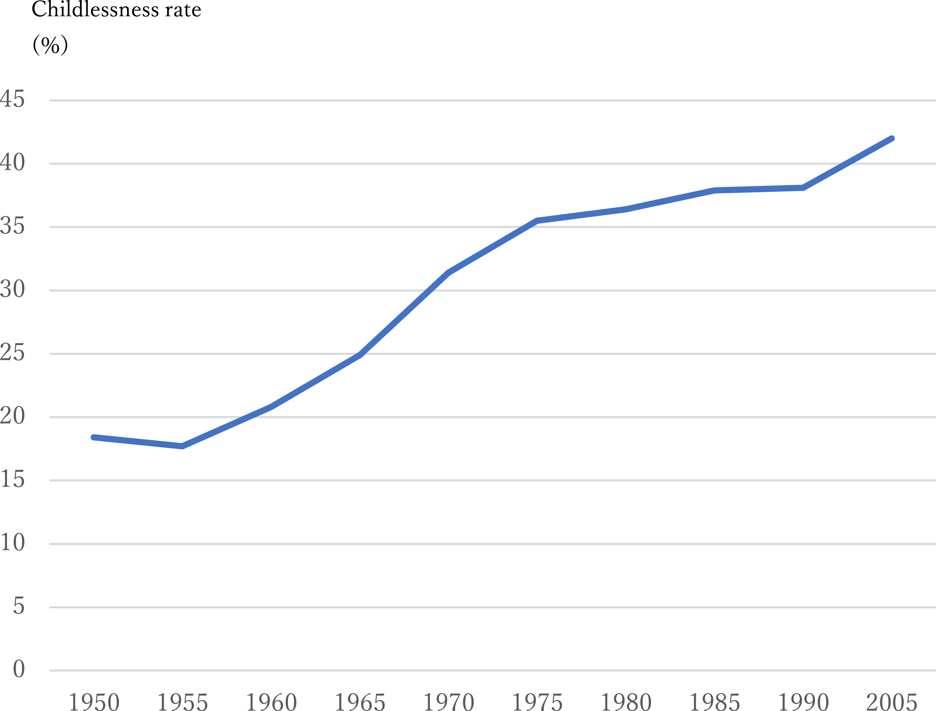
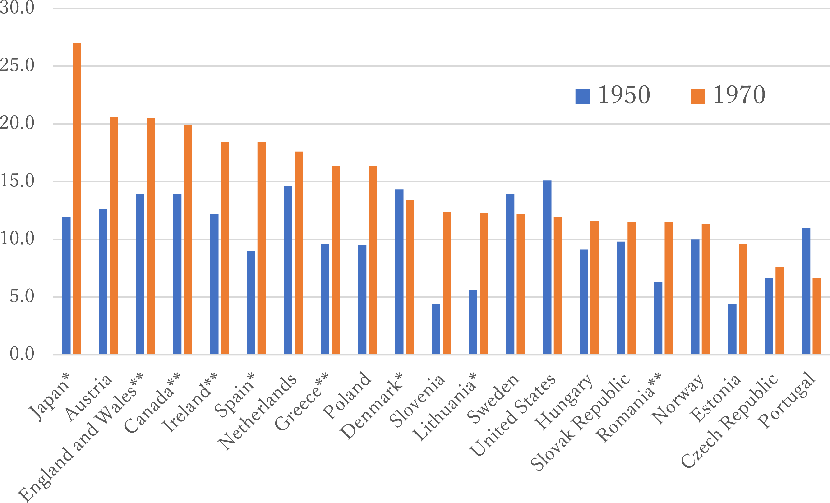
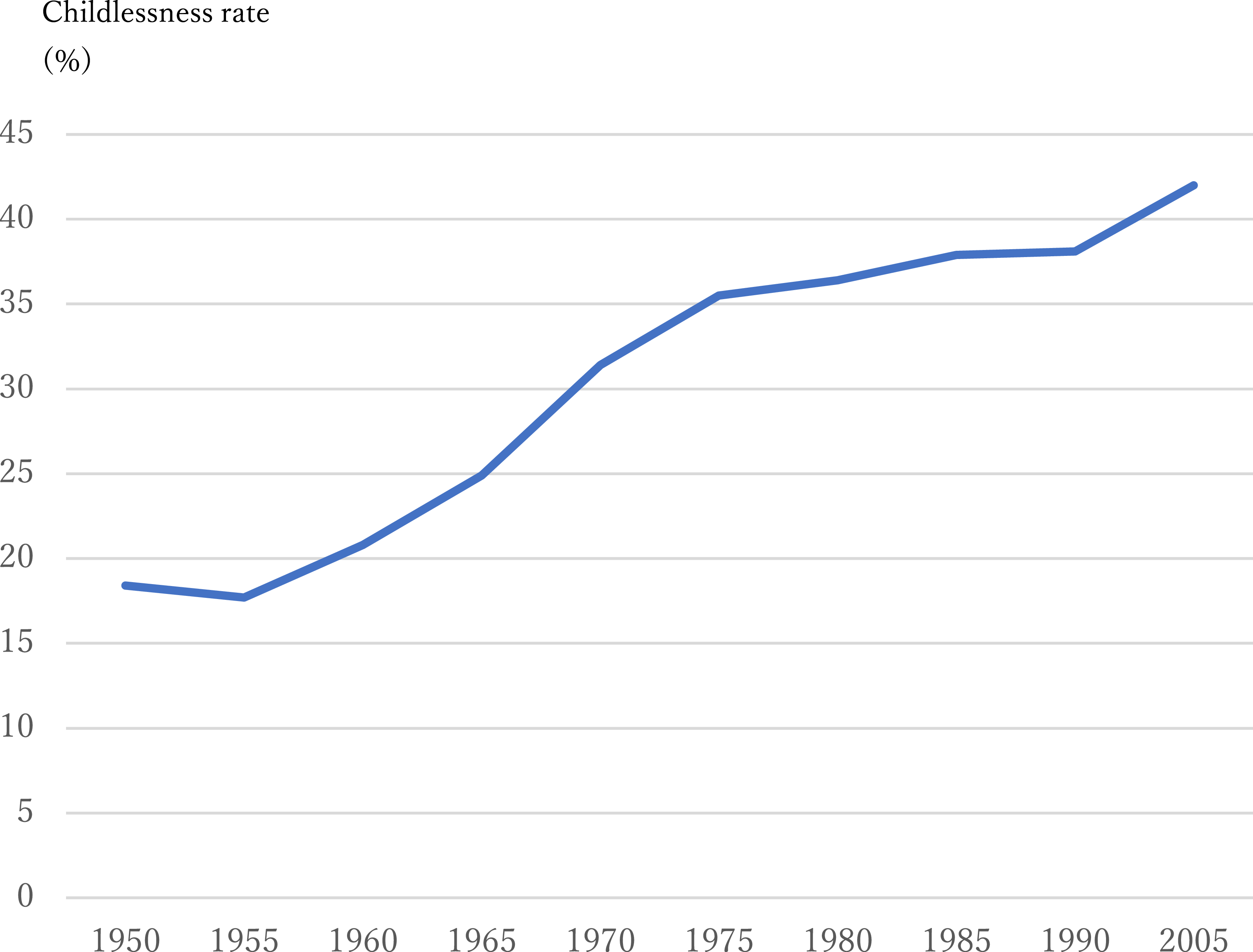
Childless women are becoming increasingly numerous in many economically developed countries. In fact, childlessness rates have increased in 17 of 21 countries sampled in Figure 1. If one specifically examines the trend in Japan, then nearly 40% of women born in 1990 and up to 50% of men and 42% of women born in 2005 are expected never to rear children during their lifetime (Figure 2).
Definitive childlessness.
(The definitive childlessness rate is defined as the proportion of childlessness among women at the end of the reproductive period. In this figure, 1950 signifies women born in 1950).
*Data of 1955 are used instead of 1950.
**Data of 1965 are used instead of 1970.
Source: OECD, human family database.

Childlessness rate in Japan.
* Proportion (%) of definitive childless women per cohort.
**Definitive childlessness rate is defined as the proportion of childlessness among women at the end of the reproductive period.
Source: National Institute of Population and Social Security Research, Japan, The Nikkei 2023.08.09.
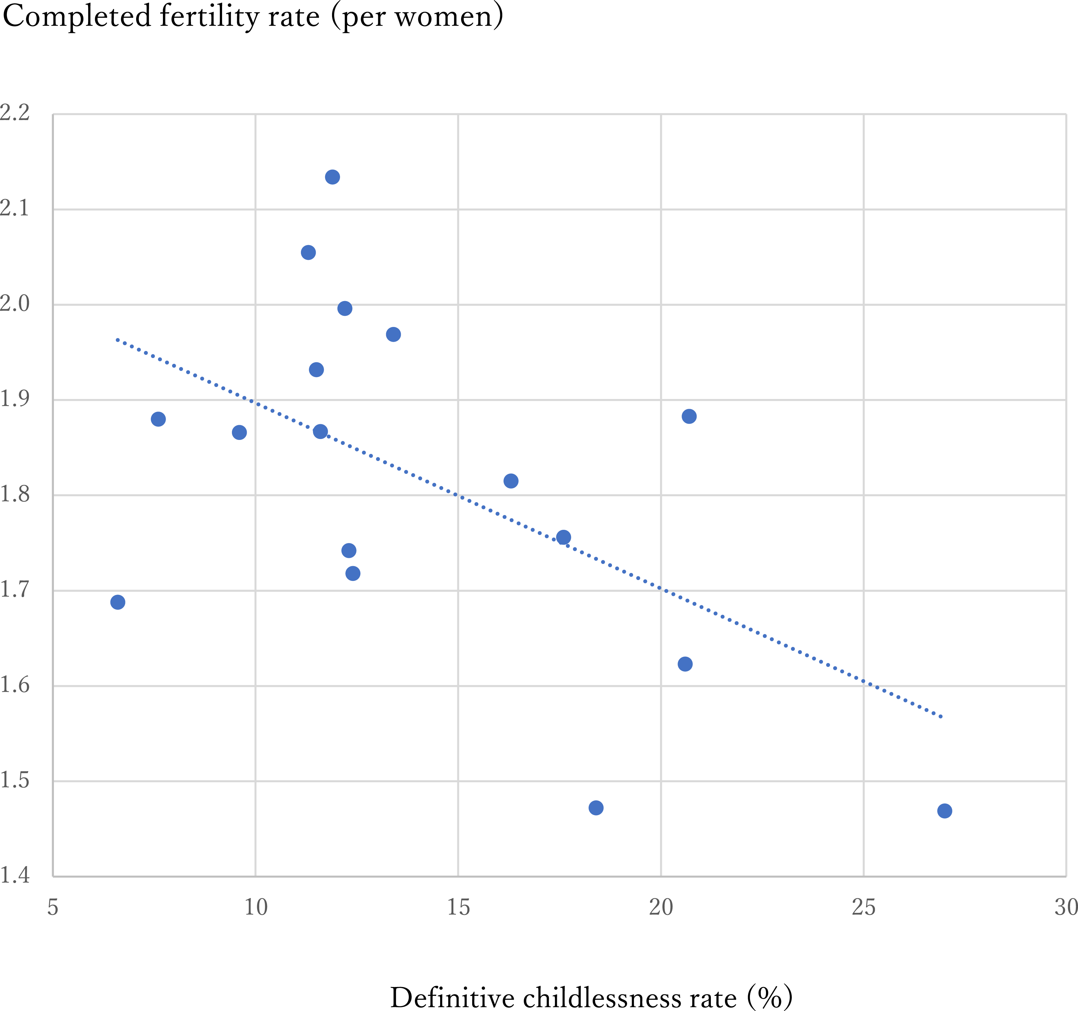
As economies develop, fertility rates typically decline. Indeed, many countries have experienced a decline in the total fertility rate during the transition from economically developing to developed countries. The increasing proportion of childless women is a crucial factor underlying the decrease in the total fertility rate in many developed countries (Figure 3).
Definitive childlessness and completed fertility rates.
(Proportion (%) of cohort definitive childless and completed fertility rates of women born in 1970).
Source: OECD, human family database.

Reducing fertility rates that are too high in economically developing countries is likely to be helpful for increasing per capita variables (e.g., capital, income, consumption). However, the concern arises in some developed countries that fertility rates, which are too low, affect the sustainability of social security. For example, the total fertility rate in Japan fell below 2 in the early 1970s and dropped to 1.26 in 2005. Although it recovered somewhat (to 1.43 in 2015), the Corona shock caused it to drop to 1.26 in 2022. At the same time, the national burden ratio rose from 38.4% in 1990 to 47.5% in 2022. Although the national burden rate increased by 9.1 percentage points, 8.2 percentage points are explained by the rising social security burden. However, because of the budget deficit in Japan, the potential national burden rate, including the budget deficit, rose to 53.5% in 2022. The change in the age structure resulting from this rapid decline in the birth rate strongly affects the economy.
Many researchers have reported economic analyses of fertility rates. One pioneer work is that of Becker (Reference Becker1960), who regarded children as a consumption good. Both the number of children as well as the propensity to consume affect utility in such an economy. Households choose a family size to maximize their utility given the relative prices of commodities, as explained by Bagozzi and van Loo (Reference Bagozzi and van Loo1978), Galor and Weil (Reference Galor and Weil1996), and others. Other important works include those reported by Becker and Barro (Reference Becker and Barro1988) and Barro and Becker (Reference Barro and Becker1989). In their model, household utility depends on the consumption level and the children’s utility. Choices of fertility and consumption derive from maximizing a dynastic utility function. Another type of setting is that in which parents expect their children’s support when they age (Zhang & Nishimura, Reference Zhang and Nishimura1989).
Gobbi (Reference Gobbi2013) provided an endogenous fertility model in which individuals have different preferences for bearing and rearing children. He demonstrates that a reduction in the gender wage gap and increased fixed costs of becoming a parent negatively affect the fertility rate and childlessness. Baudin et al. (Reference Baudin, de la Croix and Gobbi2020) insisted on two main types of childlessness: poverty-related and high opportunity-cost-related. Poverty-driven childlessness decreases as the average educational attainment level increases, but the main reason for childlessness shifts to high opportunity costs. Such studies must include an adequate discussion of the production sector and the role of saving (i.e., investment and physical capital).
Difficulties related to childlessness are integrated into a standard overlapping generations (OLG) model. Firms produce final goods using physical capital and labor. As described by Becker (Reference Becker1960) and Galor and Weil (Reference Galor and Weil1996), households’ utility depends on consumption and the number of children. Unlike those earlier reports, it is acknowledged for this study that preferences for children might differ among households. Households determine the number of children to maximize the household utility. If one uses time to rear children, then consumption decreases because the time spent on work declines. The number of children and the time spent on work differ among households because preferences for children differ among households. The effects of an increase in the childlessness rate on economic dynamics are specifically examined in this study. One can expect that an increase in the childlessness rate tends to affect many households’ utility adversely.
Moreover, the effects of a child allowance policy on household utility can be demonstrated. Many studies have specifically examined the effects of childcare support policies. Milligan (Reference Milligan2005) investigates the effect of prenatal payment policies introduced in Quebec, Canada. He finds strong evidence of their policy’s considerable effects on fertility and some heterogeneous responses. González (Reference González2013), from studies of the effect of a universal child benefit on fertility and maternal labor supply in Spain, finds that the unanticipated introduction of a sizable child benefit increases fertility significantly, partly through reduced abortions. Raute (Reference Raute2019) assesses whether income-dependent maternity leave in Germany positively affects fertility. He shows that such leave has a positive and significant effect on fertility and increases fertility by up to 23% for women with tertiary education. Laroque and Salanié (Reference Laroque and Salanié2014) report that financial incentives affect fertility decisions in France significantly.
Nevertheless, the effect of cash transfer policies on fertility found from these studies is significant but small. By contrast, Baughman and Dickert-Conlin (Reference Baughman and Dickert-Conlin2003, Reference Baughman and Dickert-Conlin2009) and Brewer et al. (Reference Brewer, Ratcliffe and Smith2011) respectively found that child benefits had no significant effect on fertility in the USA or the UK. Policies supporting childcare are not always limited to cash transfers. Bauernschuster et al. (Reference Bauernschuster, Hener and Rainer2016) demonstrated that an increase in public childcare expenditures affects fertility significantly. Their findings indicate that universal early childcare might be an effective means of increasing fertility.
Doepke and Kindermann (Reference Doepke and Kindermann2019) argue that targeted policies which specifically reduce the burden of childcare on mothers tend to have a particular effect on fertility. If one follows their argument, then non-financial support that unloads the burden on mothers (e.g., increasing the capacity of nursery schools, encouraging men to take more parental leave) is more cost-effective than financial support.
These studies investigate the impact of various child-rearing support policies on birth rates. The costs of child support policies are likely to result unavoidably in higher tax rates and higher social security contributions. Therefore, it is also necessary to discuss policy effects on people’s utility, but earlier studies have only inadequately examined households’ utility. This paper therefore specifically assesses the economic effects of the policies on utility. Because households have different preferences, the effects of policies vary from household to household. Desirable tax rates also vary widely among individuals. Nevertheless, the analysis presented herein suggests that introducing childcare support policies would have the desired effect on many households.
This paper is organized as follows. Section 2 introduces a basic model discussed herein. Section 3 derives the dynamic behavior of the economy. Section 4 presents discussion of the economic effects of an increase in the childlessness rate. Section 5 presents analyses of how childcare policy alters households’ incentives for having children and whether or not such a policy can improve household utility. Section 6 provides numerical examples. Section 7 presents a description of the conclusions obtained from this study.
2. The Model
This section presents a description of the model considered herein. The final good is homogeneous. Its production function is specified as ${Y_{it}} = AK_t^\alpha L_t^{1 - \alpha },$
where Y t represents the aggregate output,Footnote 1 A denotes the productivity parameter, K represents the capital stock, and L signifies the labor input in this sector. Moreover, 0 < α < 1 is assumed. Capital depreciates fully during the production process.
Firms maximize their profits at each date, taking interest rate r t and wage rate w t as given. From the firms’ profit maximization (evaluated market equilibrium), one can infer that $(1 + {r_t}) = A\alpha K_t^{\alpha - 1}L_t^{1 - \alpha },$ ${{{w}}_t} = {{A}}\left( {1 - \alpha } \right)K_t^\alpha L_t^{ - {{\alpha }}}.$
One can specifically examine consumers (households). Generation t is defined as people who work in period t. Individuals live for three periods. During the first period (childhood), they make no decisions. During the second period (young), they work and rear their children, if any. They also consume part of their income and save the rest. During the final period (old), they retire and consume the savings accumulated during the second period. As explained later, they also consume government services during the final period.Footnote 2
The utility of an individual in generation t (U it ) is defined as ${U_{it}} = {\rm{log}}\;{c_{it}} + {1 \over {1 + \rho }}{\rm{log}}\;{c_{it}}_{ + 1} + {\gamma _i}{\rm{log}}\;\left( {1 + a{n_{it}}} \right) + {\beta \over {1 + \rho }}{\rm{log}}\;{g_t}_{ + 1},$
where c it , c it+1, g t+1, n it , and ρ respectively represent consumption during the young and old period, the level of government services that only older people can consume, the number of children of generation t of type i,Footnote 3 and the subjective discount rate. Moreover, β > 0 and γ i > 0 are assumed. The standard demand model of household fertility behavior (Becker, Reference Becker1960; Galor & Weil, Reference Galor and Weil1996) is followed. These analyses do not address integer constraints on the number of children. Therefore, n it can be a fractional value.
Households might have a different value of γ i : preferences for children differ among households. Type i households are defined as those for which the preference for children is γ i . Presumably, γ i is distributed uniformly between 0 and γ a . Therefore, the ratio of the household of type i is given as 1/γ a .
During the second period, each household has one unit of time. The time spent on work by the individuals is 1–zn it , where z denotes the time cost to rear one child. Based on that adopted assumption, one can obtain ${c_{it + 1}} = \left( {1 + {\rm{\;}}{r_{t + 1}}} \right)\left[ {{\rm{\;}}{w_t}\left( {1 - z{\rm{\;}}{n_{it}}} \right)\left( {1 - {\rm{\;}}{\tau _t}} \right) - {c_{it}}} \right],$
where τ t denotes the tax rate. Consumers decide how much they will work and how many children they will have.Footnote 4 They also allocate disposable income between consumption and savings. They maximize their respective utilities given as equation (4) under the constraints given by equation (5), taking w t , τ t , g t+1, and r t+1 as given. From the utility maximization, one can show that ${c_{it}} = {{1 + \rho } \over {2 + \rho }}\left[ {\;{w_t}\left( {1 - z\;{n_{it}}} \right)\left( {1 - \;{\tau _t}} \right)} \right],$ ${{{{{c}}_{{{it}} + 1}}} \over {{{{c}}_{{{it}}}}}} = {{1 + \;{{{r}}_{{{t}} + 1}}} \over {1 + \rho }},$ ${n_{it}} = \;\left\{ {\matrix{0 & {\left( {{\rm{when}}\;\;{\gamma _i} \le {z \over {\Gamma a}}} \right),} \cr {{{\Gamma a{\gamma _i} - z} \over {az\left( {1 + \Gamma {\gamma _i}} \right)}}\;} & {\left( {{\rm{when}}\;\;{\gamma _i}{\rm{ \gt }}{z \over {\Gamma a}}} \right),} \cr } } \right.$
where $\Gamma \equiv {{1 + \rho } \over {2 + \rho }}$
. From equation (8), one can obtain the following proposition.
$\Gamma \equiv {{1 + \rho } \over {2 + \rho }}$
. From equation (8), one can obtain the following proposition.
Proposition 1 There exists a unique value of $\;{\gamma _i} = {z \over {\Gamma a}}$
for which households are indifferent between being childless, or not.
$\;{\gamma _i} = {z \over {\Gamma a}}$
for which households are indifferent between being childless, or not.
The number of children (n
it
) is positive if and only if ${\gamma _i}{\rm{ \gt }}{z \over {\Gamma a}}$
. Therefore,
${\gamma _i}{\rm{ \gt }}{z \over {\Gamma a}}$
. Therefore, ${z \over {\Gamma a}} \div {\gamma _a}$
× 100 =
${z \over {\Gamma a}} \div {\gamma _a}$
× 100 = ${z \over {\Gamma a{\gamma _a}}}$
× 100% of households decide to have no children. From equation (8), the fertility rate in period t (which is defined as n
t
) can be calculated as
${z \over {\Gamma a{\gamma _a}}}$
× 100% of households decide to have no children. From equation (8), the fertility rate in period t (which is defined as n
t
) can be calculated as $\!\!\!\!\!\!\!\!\!\!\!\!\!\!\!\!\!\!\!\!\!\!\!\!\!\!\!\!\!\!\!\!\!\!\!\!\!\!\!\!\!\!\!\!\!\!\!\!\!\!\!\!\!\!\!\!\!\!\!\!\!\! {n_t} = \int_{{z \over {\Gamma a}}}^{{\gamma _a}} {{1 \over {{\gamma _a}}}} {{\Gamma a{\gamma _i} - z} \over {za\left( {1 + \Gamma {\gamma _i}} \right)}}d{\gamma _i}$ $ = {1 \over {z{\gamma _a}}}\left\{ {{\gamma _a} - {z \over {\Gamma a}} - {{a + z} \over {\Gamma a}}{\rm{log}}\left( {{{a\left( {1 + \Gamma {\gamma _a}} \right)} \over {a + z}}} \right)} \right\} \equiv n.$
It is noteworthy that the definition of the total fertility rate differs from the commonly used definition because this study makes no distinction between men and women. Therefore, n denotes the number of children per adult rather than the number per woman. Consequently, 2n is the natural definition of the total fertility rate. From equation (9), an increase in the childlessness rate, defined as a decrease in γ a , decreases the total fertility rate. This finding is supported by empirical data (Figure 3).
For analytical clarity, the model focuses on the opportunity cost of time and does not explicitly incorporate expenditures on child-related goods and services. Nonetheless, part of the general consumption good can be interpreted as encompassing such goods so that direct child-rearing costs are partially absorbed within the existing framework.
The model can be extended to include explicit expenditures. Suppose that raising a child requires goods rather than parental time and that each child entails an expenditure $\;\theta {w_t}$
, reflecting labor-intensive services such as childcare and education. In this case, total fertility rate
$\;\theta {w_t}$
, reflecting labor-intensive services such as childcare and education. In this case, total fertility rate $\;{n_t}$
depends on
$\;{n_t}$
depends on $\theta $
instead of z, and if the preference for children
$\theta $
instead of z, and if the preference for children $\;{\gamma _i}$
is sufficiently small relative to
$\;{\gamma _i}$
is sufficiently small relative to $\theta $
, households optimally choose not to have children. Hence, while the role of z is effectively transferred to
$\theta $
, households optimally choose not to have children. Hence, while the role of z is effectively transferred to $\theta $
(with a different functional form), the qualitative properties of the model remain unchanged.
$\theta $
(with a different functional form), the qualitative properties of the model remain unchanged.
Thus, introducing child-related goods would primarily lead to a reinterpretation of parameters rather than altering the core mechanisms or conclusions. A more explicit treatment of these direct costs would, however, be a valuable direction for future research.
In this model, the total fertility rate depends on parameters such as z and ${\gamma _a}$
. These parameters can be interpreted more broadly to capture factors such as housing affordability and cultural factors. Housing affordability can also be incorporated within the present framework. Let h denote housing affordability, and define the per-child time cost as z = z(h) with z’(h) <0, so that greater affordability reduces the effective cost of childrearing by alleviating commuting burdens, providing adequate living space, and improving access to childcare resources. Given z’(h) <0, n increases with h. Moreover, higher housing affordability may raise the average preference for childrearing (the average value of
${\gamma _a}$
. These parameters can be interpreted more broadly to capture factors such as housing affordability and cultural factors. Housing affordability can also be incorporated within the present framework. Let h denote housing affordability, and define the per-child time cost as z = z(h) with z’(h) <0, so that greater affordability reduces the effective cost of childrearing by alleviating commuting burdens, providing adequate living space, and improving access to childcare resources. Given z’(h) <0, n increases with h. Moreover, higher housing affordability may raise the average preference for childrearing (the average value of ${\gamma _i}$
and
${\gamma _i}$
and ${\gamma _a}$
), reflecting the idea that childrearing is more attractive in supportive environments.
${\gamma _a}$
), reflecting the idea that childrearing is more attractive in supportive environments.
Cultural factors are also important. Social norms and perceived social pressures influence both the perceived cost of and motivation for having children across societies. Family expectations and the intergenerational transmission of fertility norms play a significant role (Panova et al., Reference Panova, Buber-Ennser, Bujard and Milligan2023). Moreover, parental values and the cultural orientations of their ethnic group influence perceptions of child-rearing costs and the motivation to have children (Abramson et al., Reference Abramson, Daniel and Knafo-Noam2018; Harkness & Super, Reference Harkness and Super2020). Taken together, these findings suggest that cultural factors can affect both the perceived costs of child-rearing and individual preferences for having children.
Although the model does not explicitly incorporate gender, it is useful to note how gender inequality relates to its core mechanisms. Empirical research shows that unequal divisions of unpaid care work and gendered labor market constraints effectively raise the opportunity cost of child-rearing – corresponding to a higher value of the parameter z in our framework (Casarico et al., Reference Casarico, Del Rey and Silva2023; Machado & Jaspers, Reference Machado and Jaspers2023). Gender inequality may also shape fertility preferences, thereby influencing parameter $\;{\gamma _i}$
. Evidence indicates that more egalitarian sharing of childcare and household tasks is associated with higher fertility intentions and realized births, whereas persistent inequality tends to suppress additional childbearing (Dommermuth et al., Reference Dommermuth, Hohmann-Marriott and Lappegård2017; Schober, Reference Schober2013).
$\;{\gamma _i}$
. Evidence indicates that more egalitarian sharing of childcare and household tasks is associated with higher fertility intentions and realized births, whereas persistent inequality tends to suppress additional childbearing (Dommermuth et al., Reference Dommermuth, Hohmann-Marriott and Lappegård2017; Schober, Reference Schober2013).
While these gender-specific mechanisms are abstracted from for analytical tractability, they can be interpreted as affecting z and $\;{\gamma _i}$
within our model. A fuller treatment would require gender-differentiated labor supply or intrahousehold bargaining, but such extensions would operate in the same qualitative direction and thus do not alter the main insights of the analysis.
$\;{\gamma _i}$
within our model. A fuller treatment would require gender-differentiated labor supply or intrahousehold bargaining, but such extensions would operate in the same qualitative direction and thus do not alter the main insights of the analysis.
The total labor supply in the economy can be expressed as shown below: $\eqalign{{L_t} & = {\rm{ }}\int_0^{{\gamma _a}} {{{{N_t}} \over {{\gamma _a}}}} \left( {1 - z{n_{it}}} \right)d{\gamma _i} \cr& = {{{N_t}} \over {{\gamma _a}}}\left\{ {{z \over {\Gamma a}} + {{a + z} \over {\Gamma a}}{\rm{log}}\left( {{{a\left( {1 + \Gamma {\gamma _a}} \right)} \over {a + z}}} \right)z + \left( {1 + z} \right){\rm{log}}\left( {{{1 + {\gamma _a}} \over {a + z}}} \right)} \right\} \cr& \equiv {N_t}l = {N_t}\left( {1 - zn} \right).}$
It is noteworthy that $1 - zn = l$
must hold.
$1 - zn = l$
must hold.
The government imposes a tax on wage income to provide public services for older people. This service can be regarded as medical or nursing care for older people. Furthermore, this term can be interpreted to include psychological reassurance about social security, although this is not a public pension or other government service to compensate for income.
From the government’s budget constraint, one can obtain $\;{\tau _t}\;{w_t}{L_t} = \;{N_{t - 1}}{g_t}$
, assuming a constant tax rate (this is shown to be true in the steady state). Therefore, the following expression can be made:
$\;{\tau _t}\;{w_t}{L_t} = \;{N_{t - 1}}{g_t}$
, assuming a constant tax rate (this is shown to be true in the steady state). Therefore, the following expression can be made: ${\tau _t} = \tau .$
3. Dynamic behavior of the economy
This section presents discussion of the dynamic behavior of the economy. The population dynamics are given as ${N_{t + 1}} = {\rm{\;}}{N_t}n{\rm{\;}} = {\rm{\;}}{N_t}{{{( {1 - l} )}}\over{z}}.$
Regarding capital, one can demonstrate the following. ${K_{t + 1}} = {1 \over {2 + \rho }}\left[ {\;{w_t}\;{L_t}\left( {1 - \tau } \right) - \;{C_t}} \right] = {{1 - \tau } \over {2 + \rho }}A\left( {1 - \alpha } \right)K_t^\alpha L_t^{1 - \alpha }.$
From equations (11) and (12), it can be shown that $\;{k_{t + 1}} = {{A\left( {1 - \alpha } \right)\left( {1 - \tau } \right)} \over {\left( {2 + \rho } \right)n}}\;k_t^\alpha {l^{1 - \alpha }.}$
where k t ≡ K t /N t. One can then readily demonstrate that k t converges monotonically to a unique steady state. From equation (13), one can find ${k^{\rm{*}}} \equiv {\left( {{{A\left( {1 - \alpha } \right)\left( {1 - \tau } \right)} \over {n\left( {2 + \rho } \right)}}} \right)^{{1 \over {1 - \alpha }}}}l. $
in the steady state, where k* denotes the steady state value of k t.
4. Effects of declining birth rate on utility
This section specifically examines the steady state. The steady state is defined as a state in which every variable grows at a constant rate, which may be zero or negative. From equations (5), (6), (8), (10), and (14) and using the fact that ${k_t} = {k_{t + 1}} = {k^*}$
in the steady state, one can rewrite c
it
, c
it+1, 1+an
it
, and g
it+1 as
${k_t} = {k_{t + 1}} = {k^*}$
in the steady state, one can rewrite c
it
, c
it+1, 1+an
it
, and g
it+1 as ${c_{it}} = {\left( {{{A\left( {1 - \alpha } \right)\left( {1 - \tau } \right)} \over {2 + \rho }}} \right)^{{1 \over {1 - \alpha }}}}{n^{{{ - \alpha } \over {1 - \alpha }}}}{{a + z} \over {a\left( {1 + \Gamma {\gamma _i}} \right)}}\left( {1 + \rho } \right),$ ${c_{it + 1}} = A\alpha {n^{{{1 - 2\alpha } \over {1 - \alpha }}}}{\left( {{{A\left( {1 - \alpha } \right)\left( {1 - \tau } \right)} \over {2 + \rho }}} \right)^{{\alpha \over {1 - \alpha }}}}{{a + z} \over {a\left( {1 + \Gamma {\gamma _i}} \right)}},$ $1 + a{n_{it}} = \left\{ {\matrix{1 & {\;\left( {{\rm{when}}\;\;{\gamma _i} \le {z \over {\Gamma a}}} \right),} \cr {\;{{\left( {a + z} \right)\Gamma {\gamma _i}} \over {z\left( {1 + \Gamma {\gamma _i}} \right)}}} & {\left( {{\rm{when}}\;\;{\gamma _i}{\rm{ \gt }}{z \over {\Gamma a}}} \right).} \cr } } \right.\;$ ${g_t} = {\left( {2 + \rho } \right)^{{{ - \alpha } \over {1 - \alpha }}}}{\left( {A\left( {1 - \alpha } \right)} \right)^{{1 \over {1 - \alpha }}}}\;\tau l{n^{\,{{1 - 2\alpha } \over {1 - \alpha }}}}{\left( {1 - \tau } \right)^{{\alpha \over {1 - \alpha }}}} \equiv g.$
A government sets the tax rate to maximize its objective function. It is assumed that government is short-lived and that its objective function is defined as the average utility of young and old households. Therefore, the government sets the tax rate to maximize the following equation. $\mathop \int \nolimits_0^{{\gamma _a}} {U_{it - 1}}d{\gamma _i} + n\mathop \int \nolimits_0^{{\gamma _a}} {U_{it}}d{\gamma _i}.$
These analyses assume rational expectations and myopic decision-making. Rational expectations mean that the short-lived government can estimate the tax rate accurately in the subsequent period. Myopic decision-making implies that the government does not consider the effects of current policies on future political decisions. These assumptions imply that the government chooses tax rate τ t taking τ t+1 (the tax rate in the subsequent period) as given (Meijdam & Verbon, Reference Meijdam and Verbon1996; Verbon & Verhoeven, Reference Verbon and Verhoeven1992). The tax rate is derived as ${\tau _t} = {{\beta \left( {1 - \alpha } \right)\left( {1 + \rho } \right)} \over {\left( {1 + \alpha + \rho } \right)n + \beta \left( {1 + \rho } \right)}} \equiv \tau. \;$
As presented above, equation (19) implies a constant tax rate over time because n is constant.
Herein, U i is used instead of U it because the utility of each generation remains unchanged in the steady state.
Here, the effect of an increase in the childlessness rate on household utility is considered. The childlessness rate depends strongly on ${\gamma _a}$
. We therefore conduct a comparative static analysis of how an increase in the childlessness rate (resulting from a decrease in
${\gamma _a}$
. We therefore conduct a comparative static analysis of how an increase in the childlessness rate (resulting from a decrease in ${\gamma _a}$
) affects household utility. Given the distribution of
${\gamma _a}$
) affects household utility. Given the distribution of ${\gamma _i}$
assumed in this paper, such changes reduce the average (or median) number of children per household and increase the share of childless households. While
${\gamma _i}$
assumed in this paper, such changes reduce the average (or median) number of children per household and increase the share of childless households. While ${\gamma _i}$
reflects preferences for children, we also assume that social institutions and cultural factors influence it. Accordingly, changes in social institutions and cultural factors may affect household decisions about having children through their impact on
${\gamma _i}$
reflects preferences for children, we also assume that social institutions and cultural factors influence it. Accordingly, changes in social institutions and cultural factors may affect household decisions about having children through their impact on ${\gamma _i}$
. It can be shown that
${\gamma _i}$
. It can be shown that ${{\;\partial {U_i}} \over {\partial {\gamma _a}}} = {{\partial {U_i}} \over {\partial n}}{{\partial n} \over {\partial {\gamma _a}}},$
and that $\eqalign{& {{\partial {{{U}}_{{i}}}} \over {\partial {{n}}}} = {1 \over {\left( {1 - \alpha } \right)\left( {1 + \rho } \right)}}\Big( {\left( {1 - 2\alpha } \right)\left( {1 + \beta } \right) - \alpha \left( {1 + \rho } \right)} \Big){1 \over {{n}}} - {{\beta {{z}}} \over {\left( {1 + \rho } \right)\left( {1 - {{zn}}} \right)}} \cr & \quad\quad\quad + {{1 + \alpha \left( {1 + \beta } \right) + \rho } \over {\left( {1 - \alpha } \right)\left( {1 + \rho } \right)}}\;{{1 + \alpha + \rho } \over {\left( {1 + \alpha + \rho } \right)n + \alpha \beta \left( {1 + \rho } \right)}} \cr & \quad\quad\quad- {{1 + \alpha + \beta + \rho } \over {\left( {1 - \alpha } \right)\left( {1 + \rho } \right)}}\;{{1 + \alpha + \rho } \over {\left( {1 + \alpha + \rho } \right)n + \beta \left( {1 + \rho } \right)}}.}$
Proposition 2 An increase in the childlessness rate, defined as a decrease in γa, negatively affects all households’ utilities if and only if ${{\partial {U_t}} \over {\partial n}}$
(evaluated at equilibrium) given by equation (21) is positive.
${{\partial {U_t}} \over {\partial n}}$
(evaluated at equilibrium) given by equation (21) is positive.
The childlessness rate in this model is endogenously determined by the parameter ${\gamma _a}$
, with smaller values of
${\gamma _a}$
, with smaller values of ${\gamma _a}$
leading to higher childlessness rates. The analysis here is a comparative static exercise, examining how utility changes when
${\gamma _a}$
leading to higher childlessness rates. The analysis here is a comparative static exercise, examining how utility changes when ${\gamma _a}$
decreases and the childlessness rate correspondingly rises.
${\gamma _a}$
decreases and the childlessness rate correspondingly rises.
It is difficult to solve this inequality equation (21) analytically. Therefore, one must rely on numerical examples. Here, α is the share of capital in the production. Therefore, α is regarded as approximately 0.3. If the subjective discount rate is 2% per year and if one period is regarded as 25–30 years, then ${1 \over {\left( {1 + \rho } \right)}}$
is roughly 0.55–0.6. Therefore, ρ is assumed to be 0.7 (de la Croix & Doepke, Reference de la Croix and Doepke2003).
${1 \over {\left( {1 + \rho } \right)}}$
is roughly 0.55–0.6. Therefore, ρ is assumed to be 0.7 (de la Croix & Doepke, Reference de la Croix and Doepke2003).
Baudin et al. (Reference Baudin, de la Croix and Gobbi2020) estimated the time cost for one child as 0.188. Prettner and Werner (Reference Prettner and Werner2016) used 0.19 for their simulation. However, it is noteworthy that the preconditions of their model and ours differ. Baudin et al. (Reference Baudin, de la Croix and Gobbi2020) also considered the fixed cost of rearing children. Prettener and Werner (Reference Prettner and Werner2016) assumed other costs for education. Therefore, it might be a good idea to use a higher value of z than they used in their studies. It is assumed for this discussion that z is 0.2–0.25.
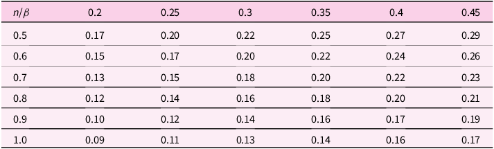
Also, β is the weight in the utility function of government service for older people. Estimating this point is not a simple matter. The value of β using the tax rate for this service is inferred as τ. Table 1 presents the relation among τ, n, and β (assuming that α = 0.3and ρ is 0.7). For the moment, β is assumed as 0.30–0.35. This assumption is generally reasonable if one assumes τ between 15% and 25% and assumes that n is 0.6–1.0.Footnote 5
Tax rates for given values of n and β

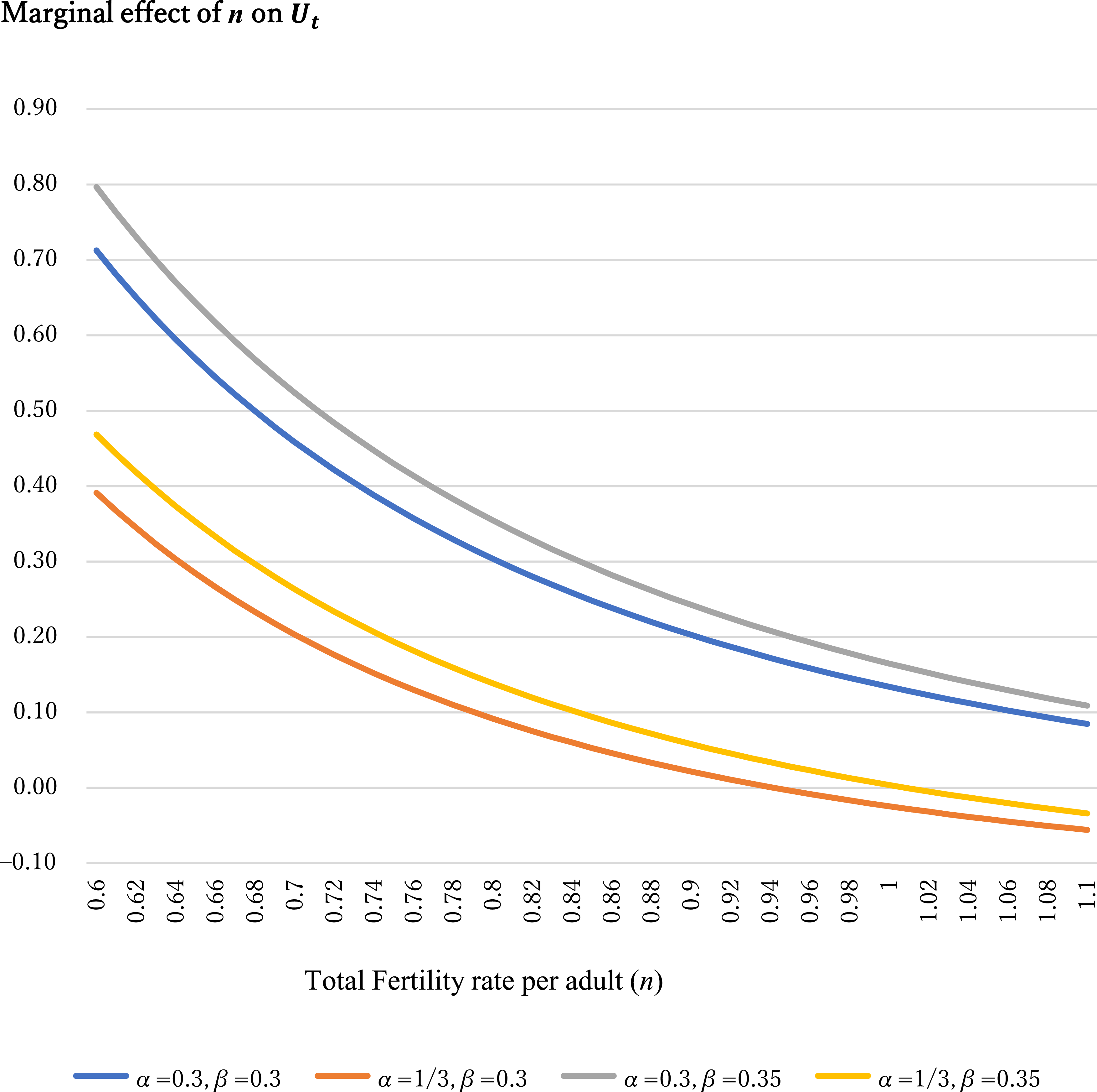
Figure 4 depicts the values of ${{\partial {U_t}} \over {\partial n}}$
for parameter values. Considering four cases, the inferences are made that α is 0.3 and 1/3 and that β is 0.3 and 0.35. This result shows that the value of
${{\partial {U_t}} \over {\partial n}}$
for parameter values. Considering four cases, the inferences are made that α is 0.3 and 1/3 and that β is 0.3 and 0.35. This result shows that the value of ${{\partial {U_t}} \over {\partial n}}$
is positive under widely various n.
${{\partial {U_t}} \over {\partial n}}$
is positive under widely various n.
Marginal effect of n on utility U t .

Economically developed countries are specifically examined for this study. In many economically developed countries, the total fertility rate is lower than the population replacement level. Data shown in Figure 4 suggest that an increase in n will likely increase utility in countries with low fertility rates. The positive effects of increased fertility on social security (lower tax rates on social security for older people and more social security) outweigh the adverse effects (although the effects depend on parameters, an increase in fertility is likely to reduce the present value of lifetime income).
5. Child allowance policy
This section presents consideration of childcare policy effects. Many studies have examined their effects (Bauernschuster et al., Reference Bauernschuster, Hener and Rainer2016; Brewer et al., Reference Brewer, Ratcliffe and Smith2011; Doepke & Kindermann, Reference Doepke and Kindermann2019; González, Reference González2013; Laroque & Salanié, Reference Laroque and Salanié2014; Milligan, Reference Milligan2005; Raute, Reference Raute2019).
This study specifically examines the effects of child care support policies on utility as well as fertility. The capital income of older people is assumed to be subject to a tax imposed by the government. Already, it has been assumed for this study that a part of the wage income of the young generation is collected to provide government services. Therefore, this policy can be regarded as income redistribution between young and old generations. The tax revenue from older people is given as ${\xi _t}A\alpha K_t^\alpha L_t^{1 - \alpha }$
if one designates the tax rate as
${\xi _t}A\alpha K_t^\alpha L_t^{1 - \alpha }$
if one designates the tax rate as ${\xi _t}.\;$
This amount is used to finance childcare support policies. Such a policy is assumed to reduce parenting time rather than providing financial assistance. Furthermore, the government was assumed to subsidize
${\xi _t}.\;$
This amount is used to finance childcare support policies. Such a policy is assumed to reduce parenting time rather than providing financial assistance. Furthermore, the government was assumed to subsidize ${w_t}{m_t}$
per child; Such policies have the same effect as reducing child-rearing time per child
${w_t}{m_t}$
per child; Such policies have the same effect as reducing child-rearing time per child $z - {m_t}$
from z.
$z - {m_t}$
from z.
It is noteworthy that ${\xi _t}A\alpha K_t^\alpha L_t^{1 - \alpha } = {w_t}{N_t}{n^m}{m_t}$
(which is equivalent to
${\xi _t}A\alpha K_t^\alpha L_t^{1 - \alpha } = {w_t}{N_t}{n^m}{m_t}$
(which is equivalent to ${\xi _t}\alpha = \left( {1 - \alpha } \right){n^m}{m_t}{{{N_t}} \over {{L_t}}}$
) must hold as a government constraint.
${\xi _t}\alpha = \left( {1 - \alpha } \right){n^m}{m_t}{{{N_t}} \over {{L_t}}}$
) must hold as a government constraint.
The budget constraint of type-i households is given as ${c_{it + 1}} = \left( {1 + {\rm{\;}}{r_{t + 1}}} \right)\left[ {{\rm{\;}}{w_t}\left( {1 - (z - {m_t}){\rm{\;}}{n_{it}}} \right)\left( {1 - {\rm{\;}}{\tau _t}} \right) - {c_{it}}} \right].$
Therefore, the household must maximize equation (4) subject to the new constraint given by equation (22). One obtains ${c_{it}} = {{1 + \rho } \over {2 + \rho }}\left[ {\;{w_t}\left( {1 - \left( {z - {m_t}} \right)\;{n_{it}}} \right)\left( {1 - \;{\tau _t}} \right)} \right],$ ${{{{c_{it + 1}}} \over {{c_{it}}}} = {{\left( {1 + \;{r_{t + 1}}} \right)\left( {1 - \;{\xi _{t + 1}}} \right)} \over {1 + \rho }}.}$ ${{n_{it}} = \left\{ {\matrix{0 & {\;\left( {{\rm{when}}\;\;{\gamma _i} \le {{z - m} \over {\Gamma a}}} \right),} \cr {{{\Gamma a{\gamma _i} - \left( {z - m} \right)} \over {a\left( {1 + \Gamma {\gamma _i}} \right)\left( {z - m} \right)}}} & {\left( {{\rm{when}}\;\;{\gamma _i}{\rm{ \gt }}{{z - m} \over {\Gamma a}}} \right).} \cr } } \right.\;\;\;}$
From equation (25), the number of children is known to increase with m
t
. Furthermore, a child allowance policy decreases the childlessness rate in the economy. Marginal households (type- ${z \over {\Gamma a}}$
households) decide to have children as a result of such a policy. The childlessness rate becomes
${z \over {\Gamma a}}$
households) decide to have children as a result of such a policy. The childlessness rate becomes ${{z - m} \over {\Gamma a{\gamma _a}}}$
. Regarding type [
${{z - m} \over {\Gamma a{\gamma _a}}}$
. Regarding type [ ${{z - m} \over {\Gamma a{\gamma _a}}}$
,
${{z - m} \over {\Gamma a{\gamma _a}}}$
, ${z \over {\Gamma a{\gamma _a}}}$
] households, they have no children before the policy is introduced. However, their marginal benefit of having children becomes predominant over the cost if the government introduces childcare support policies. The total fertility rate and labor supply are
${z \over {\Gamma a{\gamma _a}}}$
] households, they have no children before the policy is introduced. However, their marginal benefit of having children becomes predominant over the cost if the government introduces childcare support policies. The total fertility rate and labor supply are ${n_t^m = \int_{{{z - m} \over {\Gamma a}}}^{{\gamma _a}} {{1 \over {{\gamma _a}}}{{\Gamma a{\gamma _i} - z} \over {a\left( {z - m} \right)\left( {1 + \Gamma {\gamma _i}} \right)}}d{\gamma _i}}}$ $ = {1 \over {({{z}} - {{m}}){\gamma _{{a}}}}}\left\{ {{\gamma _{{a}}} - {{{{z}} - {{m}}} \over {\Gamma {{a}}}} - {{{{a}} + {{z}} - {{m}}} \over {\Gamma {{a}}}}{{log}}\left( {{{{{a}}(1 + \Gamma {\gamma _{{a}}}} \over {{{a}} + {{z}} - {{m}}}}} \right)} \right\} \equiv {{{n}}^{{m}}},$
and $\eqalign {{{L}}_{{t}}^{{m}} = & {{ }}\int_{{{{{z}} - {{m}}} \over {\Gamma {{a}}}}}^{{\gamma _{{a}}}} {{1 \over {{\gamma _{{a}}}}}{{\Gamma {{a}}{\gamma _{{i}}} - {{z}}} \over {{{a}}\left( {{{z}} - {{m}}} \right)\left( {1 + \Gamma {\gamma _{{i}}}} \right)}}{{d}}{\gamma _{{i}}}} \cr = & \,{{{{{{N}}_{{t}}}} \over {({{z}} - {{m}}){\gamma _{{a}}}}}\left\{ {{{{{z}} - {{m}}} \over {\Gamma {{a}}}} + {{{{a}} + {{z}} - {{m}}\;} \over {\Gamma {{a}}}}{{log}}\left( {{{{{a}}(1 + \Gamma {\gamma _{{a}}}} \over {{{a}} + {{z}} - {{m}}}}} \right)} \right\}}} $ $1 - {{z}}{{{n}}^{{m}}} = {{{{L}}_{{t}}^{{m}}} \over {{{{N}}_{{t}}}}} = {{{l}}^{{m}}}$
Next, the dynamic behavior of the economy is analyzed. Regarding capital, it can be shown thatFootnote 6 ${{{k}}_{{{t}} + 1}} = {{1 - {\tau _{{t}}}} \over {\left( {2 + \rho } \right){{{n}}^{{m}}}}}{{A}}\left( {1 - \alpha } \right)\;{{k}}_{{t}}^\alpha {{l}}_{{t}}^{1 - \alpha }.$
Therefore, the economy converges to a steady state monotonically. If the tax rate is assumed as constant, then the steady state value of ${k_t}$
can be expressed as presented below.
${k_t}$
can be expressed as presented below. ${{{k}}^{{*}}} \equiv {\left( {{{{{A}}\left( {1 - \alpha } \right)\left( {1 - \tau } \right)} \over {{{{n}}^{{m}}}\left( {2 + \rho } \right)}}} \right)^{{1 \over {1 - \alpha }}}}{{l}}$
In the steady state, one can rewrite c it+1, 1+an it , and g it+1 as ${{{c}}_{{{it}}}} = {\left( {{{{{A}}\left( {1 - \alpha } \right)\left( {1 - \tau } \right)} \over {2 + \rho }}} \right)^{{1 \over {1 - \alpha }}}}{{{n}}^{{{ - \alpha } \over {1 - \alpha }}}}\left( {1 + \rho } \right){{{{a}} + \left( {{{z}} - {{m}}} \right)} \over {{{a}}\left( {1 + \Gamma {\gamma _{{i}}}} \right)}},$ ${{{c}}_{{{it}} + 1}} = {{A}}\alpha {{{n}}^{{{1 - 2\alpha } \over {1 - \alpha }}}}{\left( {{{{{A}}\left( {1 - \alpha } \right)\left( {1 - \tau } \right)} \over {2 + \rho }}} \right)^{{\alpha \over {1 - \alpha }}}}{{{{a}} + \left( {{{z}} - {{m}}} \right)} \over {{{a}}\left( {1 + \Gamma {\gamma _{{i}}}} \right)}},$ $1 + {{a}}{{{n}}_{{{it}}}} = \left\{ {\matrix{1 & {\left( {{{when}}\;\;{\gamma _{{i}}} \le {{\left( {{{z}} - {{m}}} \right)} \over {\Gamma {{a}}}}} \right),} \cr {\;{{\left( {{{a}} + {{z}} - {{m}}} \right)\Gamma {\gamma _{{i}}}} \over {\left( {{{z}} - {{m}}} \right)\left( {1 + \Gamma {\gamma _{{i}}}} \right)}}} & {\left( {{{when}}\;\;{\gamma _{{i}}}{{ \gt }}{{\left( {{{z}} - {{m}}} \right)} \over {\Gamma {{a}}}}} \right),} \cr } } \right.$ ${{{g}}_{{t}}} = {\left( {2 + \rho } \right)^{{{ - \alpha } \over {1 - \alpha }}}}{\left( {{{A}}\left( {1 - \alpha } \right)} \right)^{{1 \over {1 - \alpha }}}}\tau {{{l}}^{{m}}}{{{n}}^{{{1 - 2\alpha } \over {1 - \alpha }}}}{\left( {1 - \tau } \right)^{{\alpha \over {1 - \alpha }}}} \equiv {{g}}{{.}}$
So far, we have assumed that the government provides ${w_t}{m_t}$
in subsidies per child. However,
${w_t}{m_t}$
in subsidies per child. However, ${m_t}$
can be interpreted more broadly. Parental leave, for instance, functions as a partial replacement for forgone earnings (denoted
${m_t}$
can be interpreted more broadly. Parental leave, for instance, functions as a partial replacement for forgone earnings (denoted ${{m_{t}'}}$
), and this form of compensation can be incorporated into the policy variable
${{m_{t}'}}$
), and this form of compensation can be incorporated into the policy variable ${m_t}$
. Moreover, flexible working arrangements – such as remote work, flexible schedules, or workplace childcare – effectively reduce the time requirement associated with childcare, thereby lowering the opportunity cost of child-rearing (Bratsberg and Walther, Reference Bratsberg and Walther2025). This mechanism can be represented by modifying the labor-time constraint to
${m_t}$
. Moreover, flexible working arrangements – such as remote work, flexible schedules, or workplace childcare – effectively reduce the time requirement associated with childcare, thereby lowering the opportunity cost of child-rearing (Bratsberg and Walther, Reference Bratsberg and Walther2025). This mechanism can be represented by modifying the labor-time constraint to $1 - z\left( {1 - {\varphi _t}} \right){n_t} = {l_t}$
, where a higher degree of work flexibility (
$1 - z\left( {1 - {\varphi _t}} \right){n_t} = {l_t}$
, where a higher degree of work flexibility ( ${\varphi _t}$
) reduces the effective time cost
${\varphi _t}$
) reduces the effective time cost $z\left( {1 - {\varphi _t}} \right)$
. If we define
$z\left( {1 - {\varphi _t}} \right)$
. If we define $z{\varphi _t} = {{m_t''}}$
, and
$z{\varphi _t} = {{m_t''}}$
, and ${m_t}$
in our model includes the factor of
${m_t}$
in our model includes the factor of ${{m_t''}}$
, then our model can be reformulated in terms of this setting. Accordingly,
${{m_t''}}$
, then our model can be reformulated in terms of this setting. Accordingly, ${m_t}$
can be interpreted as a composite policy measure encompassing parental leave benefits, work flexibility, and related childcare support measures.
${m_t}$
can be interpreted as a composite policy measure encompassing parental leave benefits, work flexibility, and related childcare support measures.
6. Numerical example
This subsection presents an examination of the relation between U
i
and m. Households of five types are compared, for which the values of γ
i
are ${\gamma _a},\;{{2{\gamma _a}} \over 3},\;{{{\gamma _a}} \over 2},{{{\gamma _a}} \over 3},\;{\rm{and}}\;{z \over {\Gamma a}}.$
Here, γ
a
is the highest value of γ
i
(households with the highest preference for children); γ
a
/2 is the median. The government maximizes the utility of (γ
a
/2)-type households if one employs the median voter theorem (MVT). Type
${\gamma _a},\;{{2{\gamma _a}} \over 3},\;{{{\gamma _a}} \over 2},{{{\gamma _a}} \over 3},\;{\rm{and}}\;{z \over {\Gamma a}}.$
Here, γ
a
is the highest value of γ
i
(households with the highest preference for children); γ
a
/2 is the median. The government maximizes the utility of (γ
a
/2)-type households if one employs the median voter theorem (MVT). Type ${z \over {\Gamma a}}$
refers to the marginal households that began to rear children after the policy was introduced. Type j households, those for which j is less than
${z \over {\Gamma a}}$
refers to the marginal households that began to rear children after the policy was introduced. Type j households, those for which j is less than ${{z - m} \over {\Gamma a}}$
, do not choose to rear children even if such a policy is introduced.
${{z - m} \over {\Gamma a}}$
, do not choose to rear children even if such a policy is introduced.
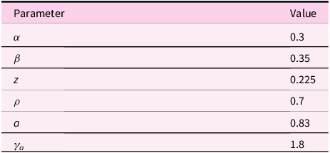
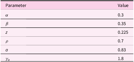
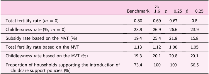
Parameter values are assumed as α = 0.3, β = 0.35, z = 0.225, ρ = 0.7, a = 0.3, and γ a = 1.8 in the benchmark case (Table 2). Table 2 presents the optimal subsidy rate for each household. Under these parameter restrictions, the total fertility rate is 0.80: approximately 24% of households have no children before the government introduces childcare support policies. It can also be confirmed that the optimal subsidy rate differs among households because the child allowance policy effects on utility differ among households. Households with a higher value of γ i can benefit more from that policy. A higher value of γ i is directly associated with a higher optimal tax rate.
Parameter values (benchmark)
It can also be calculated that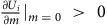 ${{\partial {U_i}} \over {\partial m}}{|_{m\; = \;0}}\; \gt \;0$
if
${{\partial {U_i}} \over {\partial m}}{|_{m\; = \;0}}\; \gt \;0$
if ${\gamma _i}{\rm{ \gt }}0.4779.$
In this case, approximately 73.4 of the population would benefit from the introduction of such childcare support policies (evaluated at m = 0).Footnote
7
${\gamma _i}{\rm{ \gt }}0.4779.$
In this case, approximately 73.4 of the population would benefit from the introduction of such childcare support policies (evaluated at m = 0).Footnote
7
The optimal subsidy rate varies across households (see Table 3). Under the median voter theorem, the government-determined subsidy rate is 19.4%, which corresponds to a tax rate of approximately 14.5%. In that case, the total fertility rate (per person) increases to 1.13 from 0.80. The childlessness rate decreases to 19.3% from 23.9%. Following the approach of Baudin et al. (Reference Baudin, de la Croix and Gobbi2020), we conducted the calculation using the baseline parameters and MVT-based tax rates. Childcare support policies induce a certain proportion of childless households to have children. This increase in households with children raises n by approximately 0.097, accounting for about 30% of the total increase.
Table 4 presents results obtained for different parameter values. For example, if γ a 1.6,Footnote 8 then the fertility rate would be 0.69. The childlessness rate would be approximately 27% without childcare support policies. It is particularly interesting that all households support the introduction of the child care support policy (evaluated at m = 0). The subsidy rate is 25.4% under the presumption that the median voter theorem holds. The fertility rate would be 1.12. The childlessness rate would be approximately 20.1%.
Optimal subsidy rate for each type of household

Note: Parameter values are given in Table 2.
Steady state equilibrium
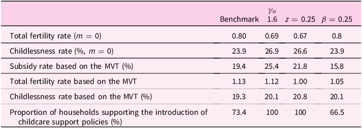
A case in which the child care cost z takes a higher value (z = 0.25) can also be shown. In this case, the fertility rate would be 0.67. The childlessness rate would be approximately 27%. As in the case above (γ a = 1.6), all households support the introduction of a childcare support policy. The subsidy rate would be 21.8% if one were to impose the median voter theory. The fertility rate would be 1.00. The childlessness rate would be approximately 20.8%.
Finally, another case is considered: the case of low preferences for social security policies during old age. One can consider the case in which β = 0.25. The proportion of households supporting the introduction of childcare support policies is 66.5%, which is lower than in the two cases above. The subsidy rate derived from the median voter theory is 15.8%. The fertility rate would increase from 0.80 to 1.05. The childlessness rate would decrease from 23.9% to 20.1%.
Household heterogeneity in preferences for children implies that child-rearing support policies affect utility differently across households. Even childless households may benefit indirectly, since these policies improve public services for older people.
7. Concluding remarks
As described herein, a simple growth model is constructed to examine how an increase in the childlessness rate affects economic dynamics and household utility levels. The results demonstrate that an increase in the childlessness rate reduces the total fertility rate of the economy and that a high childlessness rate in a steady state tends to diminish household utility. Although a lower fertility rate increases the wage rate, it reduces interest rates, raises tax rates, and leads to less adequate social security services. The adverse effects outweigh the positive ones.
Next, the effect of the child allowance policy on household utility is examined. The main conclusions are the following, assuming that rational parameter constraints are imposed. First, the marginal effects of such policies are likely to be positive for many households that already have children. However, for households without children or with few children, the benefits of such a policy are limited. The total effects tend to be negative. Second, the desired tax rate for households varies widely. For households with low preferences for children and therefore those which choose not to have children, the optimal tax rate for child support policies is zero. However, the optimal tax rate for households with more children tends to be significantly higher. Third, introducing childcare support policies is likely to be favorable for a large number of households (approximately 73% for the benchmark case presented herein).
Acknowledgements
Earlier versions of this paper were presented at the 62nd ERSA (European Regional Science Association) Congress held at the University of Alicante, Spain, and the Autumn Meeting of the Japan Association for Applied Economics held at Keio University, Tokyo, Japan. The author is grateful to Professor Michael Betz, Professor Masaya Yasuoka, and other participants at these conferences for their helpful comments. Any remaining errors are the sole responsibility of the author. This work was supported by JSPS KAKENHI Grant Numbers 24K04849 and 18K01585.







 Open access

