








1 Introduction
The inequality of Weyl provides non-trivial estimates for exponential sums having real polynomial arguments summed over all integers of an interval. In this memoir, we show that certain subsets of the natural numbers, that we term subconvex
$L^p$
 -sets, satisfy analogues of Weyl’s inequality losing nothing by comparison with the strength of these classical bounds. These bounds will facilitate applications of the Hardy-Littlewood (circle) method to problems involving subconvex
$L^p$
-sets, satisfy analogues of Weyl’s inequality losing nothing by comparison with the strength of these classical bounds. These bounds will facilitate applications of the Hardy-Littlewood (circle) method to problems involving subconvex
$L^p$
 -sets. We illustrate our ideas by considering equidistribution results for sequences of polynomials modulo
$1$
-sets. We illustrate our ideas by considering equidistribution results for sequences of polynomials modulo
$1$
 , and averages of arithmetic functions, in which the underlying arguments are restricted to subconvex
$L^p$
, and averages of arithmetic functions, in which the underlying arguments are restricted to subconvex
$L^p$
 -sets. In view of our new conclusions, the investigation and characterisation of subconvex
$L^p$
-sets. In view of our new conclusions, the investigation and characterisation of subconvex
$L^p$
 -sets are tasks that seem worthy of future attention.
We now introduce the sets central to our discussion. Throughout this memoir, when
$\mathscr A\subseteq \mathbb N$
 and
$N\geqslant 1$
and
$N\geqslant 1$
 , we write
$\mathscr A(N)=\mathscr A\cap [1,N]$
, we write
$\mathscr A(N)=\mathscr A\cap [1,N]$
 and
$A(N)=\text {card}(\mathscr A(N))$
and
$A(N)=\text {card}(\mathscr A(N))$
 . As usual, we write
$e(z)$
. As usual, we write
$e(z)$
 for
$e^{2\pi \mathrm {i}z}$
for
$e^{2\pi \mathrm {i}z}$
 . Then, when p is a positive real number, we define the mean value

Definition 1.1. Suppose that
$\mathscr A$
 is a non-empty subset of
$\mathbb N$
is a non-empty subset of
$\mathbb N$
 .
.
-
(a) We say that $\mathscr A$
 is a weakly subconvex
$L^p$
-set if
$0<p<2$
and, for all
$\varepsilon>0$
and all real numbers N sufficiently large in terms of p and
$\varepsilon $
, one has (1.2) $$ \begin{align} I_p(N;\mathscr A)\ll N^{\varepsilon -1}A(N)^p. \end{align} $$
is a weakly subconvex
$L^p$
-set if
$0<p<2$
and, for all
$\varepsilon>0$
and all real numbers N sufficiently large in terms of p and
$\varepsilon $
, one has (1.2) $$ \begin{align} I_p(N;\mathscr A)\ll N^{\varepsilon -1}A(N)^p. \end{align} $$
-
(b) We say that $\mathscr A$
is a strongly subconvex
$L^p$
-set if
$0<p<2$
and, for all real numbers N sufficiently large in terms of p, one has (1.3) $$ \begin{align} I_p(N;\mathscr A)\ll N^{-1}A(N)^p. \end{align} $$


We make three simple observations concerning this definition. First, we note that any strongly subconvex
$L^p$
 -set
$\mathscr A$
-set
$\mathscr A$
 has positive lower density. For if
$0<p<2$
has positive lower density. For if
$0<p<2$
 , it follows from (1.1) via orthogonality, a trivial estimate and the upper bound (1.3) that

Thus, we infer that
$A(N)\gg N$
 . The lower bound
$A(N)\gg N^{1-\varepsilon }$
. The lower bound
$A(N)\gg N^{1-\varepsilon }$
 follows in like manner from (1.2) for weakly subconvex
$L^p$
follows in like manner from (1.2) for weakly subconvex
$L^p$
 -sets
$\mathscr A$
-sets
$\mathscr A$
 .
.
Second, our use of the adjective subconvex is designed to remind the reader that the estimate (1.3) constitutes a bound beyond square-root cancellation, a claim justified by the observation that strongly subconvex
$L^p$
 -sets have positive lower density. Indeed, were the exponential sum associated with
$\mathscr A$
-sets have positive lower density. Indeed, were the exponential sum associated with
$\mathscr A$
 to exhibit only square-root cancellation for a set of arguments
$\alpha $
to exhibit only square-root cancellation for a set of arguments
$\alpha $
 inside the integral (1.1) having positive measure, we would have
$I_p(N;\mathscr A)\gg A(N)^{p/2}\gg N^{p/2}$
inside the integral (1.1) having positive measure, we would have
$I_p(N;\mathscr A)\gg A(N)^{p/2}\gg N^{p/2}$
 . Since
$p/2>p-1$
. Since
$p/2>p-1$
 when
$0<p<2$
when
$0<p<2$
 , it is apparent that the upper bound (1.3) is in this sense subconvex. Similar observations apply, mutatis mutandis, to weakly subconvex
$L^p$
, it is apparent that the upper bound (1.3) is in this sense subconvex. Similar observations apply, mutatis mutandis, to weakly subconvex
$L^p$
 -sets.
Third, it is apparent that when
$|\alpha |\leqslant 1/(100N)$
 , one has

Thus, we deduce from (1.1) that for
$0<p<2$
 , one has
$I_p(N;\mathscr A)\gg N^{-1}A(N)^p$
, one has
$I_p(N;\mathscr A)\gg N^{-1}A(N)^p$
 . The hypothesised upper bound (1.3) is consequently the best achievable for a p-th moment. In this context, we note that when
$0<p<1$
. The hypothesised upper bound (1.3) is consequently the best achievable for a p-th moment. In this context, we note that when
$0<p<1$
 , the upper bound (1.3) is irritatingly strong, since then one has
$I_p(N)=o(1)$
, the upper bound (1.3) is irritatingly strong, since then one has
$I_p(N)=o(1)$
 as
$N\rightarrow \infty $
as
$N\rightarrow \infty $
 . We stress that this scenario is included within the definition solely for the sake of completeness. Indeed, it is a consequence of the resolution of Littlewood’s problem (see Konyagin [Reference Konyagin18] and McGehee, Pigno and Smith [Reference McGehee, Pigno and Smith20, Corollary 1]) that
$I_1(N;\mathscr A)\gg \log A(N)$
. We stress that this scenario is included within the definition solely for the sake of completeness. Indeed, it is a consequence of the resolution of Littlewood’s problem (see Konyagin [Reference Konyagin18] and McGehee, Pigno and Smith [Reference McGehee, Pigno and Smith20, Corollary 1]) that
$I_1(N;\mathscr A)\gg \log A(N)$
 . Thus, if it were to be the case that
$\mathscr A$
. Thus, if it were to be the case that
$\mathscr A$
 is a strongly subconvex
$L^p$
is a strongly subconvex
$L^p$
 -set with
$0<p\leqslant 1$
-set with
$0<p\leqslant 1$
 , then one would have

whence
$A(N)\gg N\log A(N)$
 . Since we may assume that
$\mathscr A$
. Since we may assume that
$\mathscr A$
 has positive lower density, we obtain a contradiction. Thus, there exist no strongly subconvex
$L^p$
has positive lower density, we obtain a contradiction. Thus, there exist no strongly subconvex
$L^p$
 -sets when
$0<p\leqslant 1$
-sets when
$0<p\leqslant 1$
 . Our focus in this memoir lies with those situations in which
$1\leqslant p<2$
. Our focus in this memoir lies with those situations in which
$1\leqslant p<2$
 . It is this latter range of p for which we describe applications herein, and for which we envision the development of a coherent theory. The reader will lose nothing by assuming henceforth that p is constrained to lie in this range.
It might seem that subconvex
$L^p$
 -sets, whether weak or strong, are subsets of the integers having such special properties that they should be difficult to find, and might not perhaps occur in nature. As we explain in §§2 and 3, however, examples of subconvex
$L^p$
-sets, whether weak or strong, are subsets of the integers having such special properties that they should be difficult to find, and might not perhaps occur in nature. As we explain in §§2 and 3, however, examples of subconvex
$L^p$
 -sets are abundant. The set of all natural numbers
$\mathbb N$
-sets are abundant. The set of all natural numbers
$\mathbb N$
 is a trivial example of a weakly subconvex
$L^1$
is a trivial example of a weakly subconvex
$L^1$
 -set which is also a strongly subconvex
$L^p$
-set which is also a strongly subconvex
$L^p$
 -set whenever
$p>1$
-set whenever
$p>1$
 . This follows from the well-known bounds

We remind the reader of these familiar bounds, and their proofs, in Theorem 2.1 and the ensuing discussion. Consider next, when
$r\geqslant 2$
 , the set
$\mathscr N_r$
, the set
$\mathscr N_r$
 of r-free numbers, defined by

It transpires that
$\mathscr N_r$
 is a weakly subconvex
$L^{1+1/r}$
is a weakly subconvex
$L^{1+1/r}$
 -set, and when
$p>1+1/r$
-set, and when
$p>1+1/r$
 it is a strongly subconvex
$L^p$
it is a strongly subconvex
$L^p$
 -set. Indeed, if we write
$\mu _r(n)$
-set. Indeed, if we write
$\mu _r(n)$
 for the characteristic function of
$\mathscr N_r$
for the characteristic function of
$\mathscr N_r$
 , then these assertions follow from the work of Keil [Reference Keil17, Theorem 1.2] showing that

and

In §2 we exhibit other examples of subconvex
$L^p$
 -sets, and in §3 we show how new examples of subconvex
$L^p$
-sets, and in §3 we show how new examples of subconvex
$L^p$
 -sets may be derived from known examples.
We turn in §§4 and 5 to the topic of Weyl sums. When
$k\geqslant 2$
 and
$\alpha _i\in \mathbb R\ (0\leqslant i\leqslant k)$
and
$\alpha _i\in \mathbb R\ (0\leqslant i\leqslant k)$
 , consider the polynomial

and define the exponential sum

Suppose that the leading coefficient
$\alpha _k$
 of
$\psi (x;\boldsymbol \alpha )$
of
$\psi (x;\boldsymbol \alpha )$
 has the kind of Diophantine approximation made available via Dirichlet’s theorem, so that
$a\in \mathbb Z$
has the kind of Diophantine approximation made available via Dirichlet’s theorem, so that
$a\in \mathbb Z$
 and
$q\in \mathbb N$
and
$q\in \mathbb N$
 satisfy
$(a,q)=1$
satisfy
$(a,q)=1$
 and
$|\alpha _k-a/q|\leqslant 1/q^2$
and
$|\alpha _k-a/q|\leqslant 1/q^2$
 . In these circumstances, it follows from Weyl’s inequality (see [Reference Vaughan24, Lemma 2.4], for example) that for each
$\varepsilon>0$
. In these circumstances, it follows from Weyl’s inequality (see [Reference Vaughan24, Lemma 2.4], for example) that for each
$\varepsilon>0$
 and each large real number N, one has

When the variables n defining the summation in (1.7) are restricted to lie in arithmetically interesting subsequences of the integers, such as the prime numbers or square-free numbers, the strength of available estimates analogous to (1.8) typically degrades substantially. Our first result on Weyl’s inequality shows that no significant degradation need be tolerated for such subsequences as those defined by weakly subconvex
$L^p$
 -sets, at least when
$k\geqslant 3$
-sets, at least when
$k\geqslant 3$
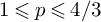
 and
$1\leqslant p\leqslant 4/3$
and
$1\leqslant p\leqslant 4/3$
 .
.
Theorem 1.2. Suppose that
$\mathscr A$
 is a weakly subconvex
$L^p$
is a weakly subconvex
$L^p$
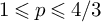
 -set for some real number p with
$1\leqslant p\leqslant 4/3$
-set for some real number p with
$1\leqslant p\leqslant 4/3$
 , and
$k\geqslant 3$
, and
$k\geqslant 3$
 . Let
$(\alpha _0,\alpha _1,\ldots ,\alpha _k)\in \mathbb R^{k+1}$
. Let
$(\alpha _0,\alpha _1,\ldots ,\alpha _k)\in \mathbb R^{k+1}$
 , and suppose that
$a\in \mathbb Z$
, and suppose that
$a\in \mathbb Z$
 and
$q\in \mathbb N$
and
$q\in \mathbb N$
 satisfy
$(a,q)=1$
satisfy
$(a,q)=1$
 and
$|\alpha _k-a/q|\leqslant 1/q^2$
and
$|\alpha _k-a/q|\leqslant 1/q^2$
 . Then, for each
$\varepsilon>0$
. Then, for each
$\varepsilon>0$
 and each large real number N, one has

A comparison of (1.8) and (1.9) will assure the reader that no degradation has occurred here accompanying our restriction of the set of summands to the subconvex
$L^p$
 -set
$\mathscr A$
-set
$\mathscr A$
 . Theorem 1.2 is in fact a corollary of a more general conclusion applicable also to the situations in which
$k\geqslant 2$
. Theorem 1.2 is in fact a corollary of a more general conclusion applicable also to the situations in which
$k\geqslant 2$
 and
$\mathscr A$
and
$\mathscr A$
 is any subconvex
$L^p$
is any subconvex
$L^p$
 -set with
$1\leqslant p<2$
-set with
$1\leqslant p<2$
 . In order to describe this result, we introduce the exponents

and

Theorem 1.3. Suppose that
$\mathscr A$
 is a weakly subconvex
$L^p$
is a weakly subconvex
$L^p$
 -set for some real number p with
$1\leqslant p<2$
-set for some real number p with
$1\leqslant p<2$
 , and
$k\geqslant 2$
, and
$k\geqslant 2$
 . Let
$(\alpha _0,\alpha _1,\ldots ,\alpha _k)\in \mathbb R^{k+1}$
. Let
$(\alpha _0,\alpha _1,\ldots ,\alpha _k)\in \mathbb R^{k+1}$
 , and suppose that
$a\in \mathbb Z$
, and suppose that
$a\in \mathbb Z$
 and
$q\in \mathbb N$
and
$q\in \mathbb N$
 satisfy
$(a,q)=1$
satisfy
$(a,q)=1$
 and
$|\alpha _k-a/q|\leqslant 1/q^2$
and
$|\alpha _k-a/q|\leqslant 1/q^2$
 . Then, for each
$\varepsilon>0$
. Then, for each
$\varepsilon>0$
 and each large real number N, one has

where
$\omega _p(k)=\max \{ \sigma _p(k),\tau _p(k)\}$
 .
.
We observe that when
$k\geqslant 3$
 and
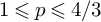
$1\leqslant p\leqslant 4/3$
and
$1\leqslant p\leqslant 4/3$
 , then the conclusion of Theorem 1.3 matches Weyl’s inequality (1.8) in strength. Moreover, when
$k\geqslant 3$
, then the conclusion of Theorem 1.3 matches Weyl’s inequality (1.8) in strength. Moreover, when
$k\geqslant 3$
 and
and

this theorem matches in strength the analogue of Weyl’s inequality deriving from modern versions of Vinogradov’s mean value theorem (obtained, for example, by substituting the main conclusions of [Reference Bourgain, Demeter and Guth6] or [Reference Wooley29] into [Reference Vaughan24, Theorem 5.2]). Meanwhile, even for
$k=2$
 , the strength of Theorem 1.3 approaches that of Weyl’s inequality in the limit as
$p\rightarrow 1+$
, the strength of Theorem 1.3 approaches that of Weyl’s inequality in the limit as
$p\rightarrow 1+$
 .
.
The focus of Theorems 1.2 and 1.3 is the derivation of exponential sum estimates with variables restricted to special subsequences of the natural numbers. If, instead, one is concerned solely with applications of the exponential sums, then one may attempt to incorporate the restriction to special subsequences into the methods employed following the application of conventional estimates for exponential sums. Thus, for example, the reader will find alternative approaches to the one presented in this memoir that extract conclusions in applications, avoiding impairment, when one restricts the underlying variables to be square-free, or more generally r-free. We refer the reader to [Reference Baker, Brüdern and Harman3, Theorem 2], for example, for a conclusion concerning small values of
$\|\alpha n^k\|$
 , when n is restricted to be square-free. In this latter work, one avoids direct use of the exponential sum

by applying the convolution identity

and removing the contribution of the large square factors directly. This approach achieves a conclusion for the application at hand matching its unrestricted analogue at the cost of various complications in the associated argument. The ideas underlying the proof of Theorems 1.2 and 1.3 permit such conclusions to be obtained in wider generality than hitherto, and oftentimes with greater economy of effort.
As the next application of the ideas in this memoir, in §6, we explore some consequences for the equidistribution modulo
$1$
 of polynomial sequences. Consider a real sequence
$(s_n)_{n=1}^\infty $
of polynomial sequences. Consider a real sequence
$(s_n)_{n=1}^\infty $
 and the associated fractional parts
$\{s_n\}=s_n-\lfloor s_n\rfloor $
and the associated fractional parts
$\{s_n\}=s_n-\lfloor s_n\rfloor $
 . This sequence is said to be equidistributed modulo 1 when, for each pair of real numbers a and b with
$0\leqslant a<b\leqslant 1$
. This sequence is said to be equidistributed modulo 1 when, for each pair of real numbers a and b with
$0\leqslant a<b\leqslant 1$
 , one has

Theorem 1.4. Suppose that
$\mathscr A=\{a_1,a_2,\ldots \}$
 , with
$a_1<a_2<\ldots $
, with
$a_1<a_2<\ldots $
 , is a strongly subconvex
$L^p$
, is a strongly subconvex
$L^p$
 -set with
$1\leqslant p<2$
-set with
$1\leqslant p<2$
 . Let
$k\geqslant 2$
. Let
$k\geqslant 2$
 , suppose that
$(\alpha _0,\alpha _1,\ldots ,\alpha _k)\in \mathbb R^{k+1}$
, suppose that
$(\alpha _0,\alpha _1,\ldots ,\alpha _k)\in \mathbb R^{k+1}$
 , and define the polynomial
$\psi (x;\boldsymbol \alpha )$
, and define the polynomial
$\psi (x;\boldsymbol \alpha )$
 as in (1.6). Then, provided that one at least of the coefficients
$\alpha _2,\ldots ,\alpha _k$
as in (1.6). Then, provided that one at least of the coefficients
$\alpha _2,\ldots ,\alpha _k$
 is irrational, the sequence
$\left ( \psi (a_n;\boldsymbol \alpha )\right )_{n=1}^\infty $
is irrational, the sequence
$\left ( \psi (a_n;\boldsymbol \alpha )\right )_{n=1}^\infty $
 is equidistributed modulo
$1$
is equidistributed modulo
$1$
 .
.
In Theorem 6.1 below, we provide a similar conclusion applicable to weakly subconvex
$L^p$
 -sets, subject to the condition that one at least of the coefficients
$\alpha _2,\ldots ,\alpha _k$
-sets, subject to the condition that one at least of the coefficients
$\alpha _2,\ldots ,\alpha _k$
 is of finite Diophantine type. We direct the reader to the discussion following Example 2.2 for an explanation of what it means for a real number
$\theta $
is of finite Diophantine type. We direct the reader to the discussion following Example 2.2 for an explanation of what it means for a real number
$\theta $
 to be of finite Diophantine type. For now, it suffices to remark that the set of such numbers has full measure in the real numbers, and includes all irrational real algebraic numbers. We remark also that the conclusion of Theorem 1.4 does not remain valid if one insists only that one at least of the coefficients
$\alpha _1,\ldots ,\alpha _k$
to be of finite Diophantine type. For now, it suffices to remark that the set of such numbers has full measure in the real numbers, and includes all irrational real algebraic numbers. We remark also that the conclusion of Theorem 1.4 does not remain valid if one insists only that one at least of the coefficients
$\alpha _1,\ldots ,\alpha _k$
 is irrational. An example of a strongly subconvex
$L^p$
is irrational. An example of a strongly subconvex
$L^p$
 -set is given in the discussion following the proof of Theorem 1.4 in §6 illustrating that equidistribution modulo
$1$
-set is given in the discussion following the proof of Theorem 1.4 in §6 illustrating that equidistribution modulo
$1$
 may fail for the sequence
$(\psi (a_n;\boldsymbol \alpha ))_{n=1}^\infty $
may fail for the sequence
$(\psi (a_n;\boldsymbol \alpha ))_{n=1}^\infty $
 when
$\alpha _1$
when
$\alpha _1$
 is irrational.
In §7, we offer some remarks concerning further applications of subconvex
$L^p$
 -sets
$\mathscr A$
-sets
$\mathscr A$
 to problems involving the estimation of averages of arithmetic functions restricted to
$\mathscr A$
to problems involving the estimation of averages of arithmetic functions restricted to
$\mathscr A$
 . We direct the reader to §7 for a more comprehensive account of such matters. Here, the reader will find a general theorem concerning such averages, as well as illustrative examples involving the von Mangoldt function, character sums and averages of cusp form coefficients, all restricted to subconvex
$L^p$
. We direct the reader to §7 for a more comprehensive account of such matters. Here, the reader will find a general theorem concerning such averages, as well as illustrative examples involving the von Mangoldt function, character sums and averages of cusp form coefficients, all restricted to subconvex
$L^p$
 -sets. For now, we present but one of many examples, involving the Möbius function
$\mu (n)$
-sets. For now, we present but one of many examples, involving the Möbius function
$\mu (n)$
 .
.
Theorem 1.5. Suppose that
$\mathscr A$
 is a strongly subconvex
$L^p$
is a strongly subconvex
$L^p$
 -set for some real number p with
$1\leqslant p<2$
-set for some real number p with
$1\leqslant p<2$
 . Then, whenever
$A>0$
. Then, whenever
$A>0$
 and N is sufficiently large in terms of A, one has

By applying the results of §3, for example, one finds that the hypotheses of this theorem are applicable when

or even

Finally, in §8, we record some connections between subconvex
$L^p$
 -sets and mean values associated with congruences modulo q. Our principal result in this setting is an analogue of the mean value (1.3) for strongly subconvex
$L^p$
-sets and mean values associated with congruences modulo q. Our principal result in this setting is an analogue of the mean value (1.3) for strongly subconvex
$L^p$
 -sets
$\mathscr A$
-sets
$\mathscr A$
 .
.
Theorem 1.6. Suppose that
$\mathscr A$
 is a strongly subconvex
$L^p$
is a strongly subconvex
$L^p$
 -set for some real number p with
$1<p<2$
-set for some real number p with
$1<p<2$
 . Then, whenever q is a natural number, one has

When q is smaller than N, the estimate provided by this theorem saves roughly a factor q over the trivial estimate
$N^p$
 , which is consistent with heuristics associated with congruences modulo q. Such heuristics would be easy to justify were we to be considering p-th moments with
$p\geqslant 2$
, which is consistent with heuristics associated with congruences modulo q. Such heuristics would be easy to justify were we to be considering p-th moments with
$p\geqslant 2$
 , since then orthogonality may be brought into play. The situation in Theorem 1.6 with
$1<p<2$
, since then orthogonality may be brought into play. The situation in Theorem 1.6 with
$1<p<2$
 is, unfortunately, rather more challenging. Thus, in order to establish this theorem, we are forced to bring into play purely analytic tools based on the use of the Sobolev-Gallagher inequality and the Carleson-Hunt theorem. We offer an application of Theorem 1.6 to character sum estimates restricted to subconvex
$L^p$
is, unfortunately, rather more challenging. Thus, in order to establish this theorem, we are forced to bring into play purely analytic tools based on the use of the Sobolev-Gallagher inequality and the Carleson-Hunt theorem. We offer an application of Theorem 1.6 to character sum estimates restricted to subconvex
$L^p$
 -sets in §8.
We defer a detailed account of our use of subconvex
$L^p$
 -sets in our methods deriving analogues of Weyl’s inequality to §4 below. For now, it suffices to make some abstract remarks that may offer some guidance to the reader, motivating our definition of subconvex
$L^p$
-sets in our methods deriving analogues of Weyl’s inequality to §4 below. For now, it suffices to make some abstract remarks that may offer some guidance to the reader, motivating our definition of subconvex
$L^p$
 -sets. Suppose then that
$\mathscr A$
-sets. Suppose then that
$\mathscr A$
 is a strongly subconvex
$L^p$
is a strongly subconvex
$L^p$
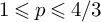
 -set for some real number p with
$1\leqslant p\leqslant 4/3$
-set for some real number p with
$1\leqslant p\leqslant 4/3$
 , and write

Consider a unimodular arithmetic function
$c:\mathbb N\rightarrow \mathbb C$
 , and write

Then it follows by orthogonality that

Thus, by applying Hölder’s inequality and the Definition 1.1(b) of a strongly subconvex
$L^p$
 -set, we find that

The
$4$
 -fold sum in the final parenthetic term may often be interpreted via Weyl differencing, or perhaps by other means. Thus, it may frequently be shown that this sum is of smaller order than the trivial estimate
$N^3$
-fold sum in the final parenthetic term may often be interpreted via Weyl differencing, or perhaps by other means. Thus, it may frequently be shown that this sum is of smaller order than the trivial estimate
$N^3$
 . In such circumstances, we conclude that one has the non-trivial estimate

We emphasise here that the arithmetic structure of the set
$\mathscr A$
 makes no appearance in this estimate beyond the estimate (1.3) that is the fundamental property of a strongly subconvex
$L^p$
makes no appearance in this estimate beyond the estimate (1.3) that is the fundamental property of a strongly subconvex
$L^p$
 -set.
-set.
We finish by highlighting some connections between the subconvex
$L^p$
 -sets of this memoir and the almost-periodic sets and sets defined by convergent sieves satisfying certain arithmetic equidistribution properties investigated by Brüdern [Reference Brüdern8] and subsequent authors (see [Reference Keil16, Reference Schlage-Puchta23]; we note that, as is made clear in the cited papers here, the work of Brüdern preceded and inspired the work of Schlage-Puchta and Keil, despite the apparent publication chronology). Given a set of natural numbers
$\mathscr A$
-sets of this memoir and the almost-periodic sets and sets defined by convergent sieves satisfying certain arithmetic equidistribution properties investigated by Brüdern [Reference Brüdern8] and subsequent authors (see [Reference Keil16, Reference Schlage-Puchta23]; we note that, as is made clear in the cited papers here, the work of Brüdern preceded and inspired the work of Schlage-Puchta and Keil, despite the apparent publication chronology). Given a set of natural numbers
$\mathscr A$
 having positive density and satisfying appropriate distribution properties in arithmetic progressions, Brüdern makes use of the orthogonality relation

together with a major arc estimation

to deliver a minor arc estimate

Such a bound would follow from the estimate (1.3) for strongly subconvex
$L^p$
 -sets
$\mathscr A$
-sets
$\mathscr A$
 whenever one has in addition the non-trivial Weyl-type bound

The bound (1.3) is not accessible to Brüdern’s almost-periodic theory without highly stringent additional conditions on the set
$\mathscr A$
 . Likewise, the estimate (1.10) does not seem to be easily accessible from the upper bound (1.3) without additional hypotheses. Thus, while there are certainly connections between the concepts of subconvex
$L^p$
. Likewise, the estimate (1.10) does not seem to be easily accessible from the upper bound (1.3) without additional hypotheses. Thus, while there are certainly connections between the concepts of subconvex
$L^p$
 -sets and Brüdern’s almost-periodic sets, the associated theories seem for now to be largely disjoint. It would be very interesting to determine if strongly subconvex
$L^p$
-sets and Brüdern’s almost-periodic sets, the associated theories seem for now to be largely disjoint. It would be very interesting to determine if strongly subconvex
$L^p$
 -sets are characterised in terms of limit-periodic structures. The author is grateful to the referee of this paper for pointing out that the problem of achieving this objective may be construed as that of obtaining an
$L^p$
-sets are characterised in terms of limit-periodic structures. The author is grateful to the referee of this paper for pointing out that the problem of achieving this objective may be construed as that of obtaining an
$L^p$
 -analogue of Brüdern’s
$L^2$
-analogue of Brüdern’s
$L^2$
 -based theory associated with limit-periodic structures.
Throughout, the letter
$\varepsilon $
 will denote a positive number. We adopt the convention that whenever
$\varepsilon $
will denote a positive number. We adopt the convention that whenever
$\varepsilon $
 appears in a statement, either implicitly or explicitly, we assert that the statement holds for each
$\varepsilon>0$
appears in a statement, either implicitly or explicitly, we assert that the statement holds for each
$\varepsilon>0$
 . Our basic parameter will be N, a sufficiently large positive number. In addition, we use
$\ll $
. Our basic parameter will be N, a sufficiently large positive number. In addition, we use
$\ll $
 and
$\gg $
and
$\gg $
 to denote Vinogradov’s well-known notation, implicit constants depending at most on
$\varepsilon $
to denote Vinogradov’s well-known notation, implicit constants depending at most on
$\varepsilon $
 , as well as other ambient parameters apparent from the context. We write
$f\asymp g$
, as well as other ambient parameters apparent from the context. We write
$f\asymp g$
 when
$f\ll g$
when
$f\ll g$
 and
$g\ll f$
and
$g\ll f$
 . Also, we define
$\|\theta \|$
. Also, we define
$\|\theta \|$
 and
$\{ \theta \}$
and
$\{ \theta \}$
 for
$\theta \in \mathbb R$
for
$\theta \in \mathbb R$
 by putting
$\|\theta \|=\min \{ |\theta -t|:t\in \mathbb Z\}$
by putting
$\|\theta \|=\min \{ |\theta -t|:t\in \mathbb Z\}$
 and
$\{ \theta \}=\theta -\lfloor \theta \rfloor $
and
$\{ \theta \}=\theta -\lfloor \theta \rfloor $
 .
.
Work on this paper was conducted while the author was supported in part by NSF grants DMS-2001549 and DMS-2502625, and Simons Fellowship in Mathematics SFM-00011955. The author is grateful to the Institute for Advanced Study, Princeton, for hosting his sabbatical, during which period this paper was completed, and to Micah Milinovich for a useful conversation associated with Corollary 7.6.
2 Examples of subconvex
$L^p$
-sets

We present a number of naturally occurring examples of subconvex
$L^p$
 -sets in this section in order to motivate our subsequent discussions. Our first result concerns the classical and well-known example of the natural numbers
$\mathbb N$
-sets in this section in order to motivate our subsequent discussions. Our first result concerns the classical and well-known example of the natural numbers
$\mathbb N$
 . Here, we justify some of the remarks made in the introduction following Definition 1.1. The proof of this theorem follows as a familiar exercise. We provide details for the sake of completeness.
Theorem 2.1. One has

and when
$p>1$
 , one has

Thus, the set
$\mathbb N$
 is a weakly subconvex
$L^1$
is a weakly subconvex
$L^1$
 -set, and when
$p>1$
-set, and when
$p>1$
 it is a strongly subconvex
$L^p$
it is a strongly subconvex
$L^p$
 -set.
-set.
Proof. Summing over the implicit geometric progression, we find that when
$\alpha \notin \mathbb Z$
 , then for integral values of N one has

Thus

and when
$p>1$
 , meanwhile,

The lower bound implicit in the first estimate of the theorem follows via a straightforward exercise using the formula (2.1), and so the conclusion of the theorem is complete.
Our second example is based on the relatively recent result of Keil [Reference Keil17, Theorem 1.2] mentioned in connection with the estimates (1.4) and (1.5).
Example 2.2. The set
$\mathscr N_r$
 of r-free numbers is a weakly subconvex
$L^{1+1/r}$
of r-free numbers is a weakly subconvex
$L^{1+1/r}$
 -set, and when
$p>1+1/r$
-set, and when
$p>1+1/r$
 it is a strongly subconvex
$L^p$
it is a strongly subconvex
$L^p$
 -set.
-set.
The final entry on our list of basic examples of subconvex
$L^p$
 -sets makes use of certain Beatty sequences. Given real numbers
$\alpha $
-sets makes use of certain Beatty sequences. Given real numbers
$\alpha $
 and
$\beta $
and
$\beta $
 , we define the Beatty set

Writing
$\mathscr B(\alpha ,\beta )=\{n_1,n_2,\ldots \}$
 with
$1\leqslant n_1<n_2<\ldots $
with
$1\leqslant n_1<n_2<\ldots $
 , this set may be interpreted as a sequence
$(n_k)_{k=1}^\infty $
, this set may be interpreted as a sequence
$(n_k)_{k=1}^\infty $
 . In order to introduce the Beatty sequences of interest to us, we recall that a real number
$\theta $
. In order to introduce the Beatty sequences of interest to us, we recall that a real number
$\theta $
 is said to be of finite Diophantine type if there is a natural number k for which

Thus, the set of real numbers not of finite Diophantine type has measure
$0$
 . Moreover, it follows from Liouville’s theorem (see [Reference Baker1, Theorem 1.1]) that every real irrational algebraic number is of finite Diophantine type.
Our estimates for moments of exponential sums over Beatty sequences are essentially as strong as those given in Theorem 2.1 for the corresponding exponential sums over all natural numbers in an interval.
Theorem 2.3. Suppose that
$\alpha $
 and
$\beta $
and
$\beta $
 are real numbers with
$\alpha>0$
are real numbers with
$\alpha>0$
 having the property that
$1/\alpha $
having the property that
$1/\alpha $
 is of finite Diophantine type. Then one has

and when
$p>1$
 , one has

Thus, the set
$\mathscr B(\alpha ,\beta )$
 is a weakly subconvex
$L^1$
is a weakly subconvex
$L^1$
 -set, and when
$p>1$
-set, and when
$p>1$
 it is a strongly subconvex
$L^p$
it is a strongly subconvex
$L^p$
 -set.
-set.
Proof. There is no loss of generality in restricting attention to the scenario in which
$\alpha>1$
 . For if
$0<\alpha \leqslant 1$
. For if
$0<\alpha \leqslant 1$
 , then the set
$\mathscr B(\alpha ,\beta )$
, then the set
$\mathscr B(\alpha ,\beta )$
 contains all large natural numbers, and the desired conclusion is essentially immediate from Theorem 2.1. Next, with our subsequent deliberations in mind, we equip ourselves with a conclusion concerning Diophantine approximations to the real number
$1/\alpha $
contains all large natural numbers, and the desired conclusion is essentially immediate from Theorem 2.1. Next, with our subsequent deliberations in mind, we equip ourselves with a conclusion concerning Diophantine approximations to the real number
$1/\alpha $
 . Since
$1/\alpha $
. Since
$1/\alpha $
 has finite Diophantine type, we may suppose that there is a natural number k with the property that

In particular, there exists a positive number
$c=c(\alpha )$
 having the property that, for all large enough natural numbers q, and for all integers a, one has

Our plan is to adopt an argument relating exponential sums over Beatty sequences to corresponding unrestricted exponential sums, following a path close to that pursued in the proof of [Reference Banks, Güloğlu and Vaughan4, Lemma 4.3]. Along the way, we incorporate adjustments and minor corrections relative to the latter source. We begin by observing that
$n=\lfloor \alpha m+\beta \rfloor $
 for some
$m\in \mathbb Z$
for some
$m\in \mathbb Z$
 if and only if

For if
$\alpha ^{-1}(n-\beta )=m-1+\delta $
 , for some
$\delta \in [0,1]$
, for some
$\delta \in [0,1]$
 and
$m\in \mathbb Z$
and
$m\in \mathbb Z$
 , then

whence

This last integer is equal to n if and only if
$0\leqslant \alpha (1-\delta )<1$
 . Thus, we have
$\lfloor \alpha m+\beta \rfloor =n$
. Thus, we have
$\lfloor \alpha m+\beta \rfloor =n$
 if and only if
$1-1/\alpha <\delta \leqslant 1$
if and only if
$1-1/\alpha <\delta \leqslant 1$
 , or equivalently, one has

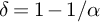
The situation with
$\delta =1-1/\alpha $
 corresponds to
$n=\alpha m+\beta -1$
corresponds to
$n=\alpha m+\beta -1$
 , whilst that with
$\delta =1$
, whilst that with
$\delta =1$
 corresponds to
$n=\alpha m+\beta $
corresponds to
$n=\alpha m+\beta $
 . Since
$\alpha $
. Since
$\alpha $
 is irrational, these scenarios can happen in their respective situations at most once.
Next, define the function
$\psi :\mathbb R\rightarrow [-1/2,1/2)$
 by putting

and observe that
$\psi (x)$
 is periodic with period
$1$
is periodic with period
$1$
 . When
$x\in [0,1)$
. When
$x\in [0,1)$
 , moreover, one has

Here, we have corrected the corresponding statement in the proof of [Reference Banks, Güloğlu and Vaughan4, Lemma 4.3]. It therefore follows from the criterion (2.3) that

where

and

The most difficult part of the decomposition (2.4) concerns the expression
$S_2(\theta )$
 . Again following [Reference Banks, Güloğlu and Vaughan4], we write

Then, by applying Montgomery and Vaughan [Reference Montgomery and Vaughan22, Lemma D.1], we see that

By Dirichlet’s approximation theorem, there exist
$a\in \mathbb Z$
 and
$q\in \mathbb N$
and
$q\in \mathbb N$
 with
$(a,q)=1$
with
$(a,q)=1$
 and
$1\leqslant q\leqslant N^k$
and
$1\leqslant q\leqslant N^k$
 satisfying the bound
$|q/\alpha -a|\leqslant N^{-k}$
satisfying the bound
$|q/\alpha -a|\leqslant N^{-k}$
 . Since
$\alpha $
. Since
$\alpha $
 has the property (2.2), we find that

whence
$q^k\geqslant cN^k$
 , and in particular
$q\gg N$
, and in particular
$q\gg N$
 . We therefore deduce from Baker [Reference Baker2, Lemma 3.2] that

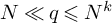
Since we may suppose that
$N\ll q\leqslant N^k$
 , we therefore see that
$W(\varphi )\ll \log (2N)$
, we therefore see that
$W(\varphi )\ll \log (2N)$
 , and hence we deduce from (2.5) that

By a change of variable, we see that

whence

We therefore deduce from (2.4) and the argument associated with Theorem 2.1 that

The first conclusion of the theorem is now immediate.
The second bound of the theorem requires additional effort. We suppose throughout that p is a real number with
$p>1$
 . We observe first that from (2.6), there is a choice of
$\eta \in \{ +1,-1\}$
. We observe first that from (2.6), there is a choice of
$\eta \in \{ +1,-1\}$
 for which

By dividing the summation over h into dyadic intervals, we find that

where
$J=\lfloor k(\log N)/(\log 2)\rfloor $
 , and
, and

Consider a typical value of
$H=2^j$
 with
$0\leqslant j\leqslant J$
with
$0\leqslant j\leqslant J$
 . By Dirichlet’s approximation theorem, there exist
$a\in \mathbb Z$
. By Dirichlet’s approximation theorem, there exist
$a\in \mathbb Z$
 and
$q\in \mathbb N$
and
$q\in \mathbb N$
 with
$(a,q)=1$
with
$(a,q)=1$
 and
$1\leqslant q\leqslant H$
and
$1\leqslant q\leqslant H$
 satisfying the bound

Since
$\alpha $
 has the property (2.2), we find that

whence
$q\gg H^{1/k}$
 . We therefore deduce from Baker [Reference Baker2, Lemma 3.2] that

Since we may suppose that
$H^{1/k}\ll q\leqslant H\ll N^k$
 , we discern that

By applying Hölder’s inequality and substituting the estimate (2.9), we find from (2.8) that

Since we are assuming throughout that
$p>1$
 , it follows via a change of variable that

where we write
$\delta =1/(8k)$
 .
.
We now return to (2.7), observing that an additional application of Hölder’s inequality reveals that

By applying (2.10), we therefore infer that

Finally, on substituting this bound into a consequence of the decomposition (2.4), we arrive at the upper bound

The second conclusion of the theorem is now immediate from the second estimate of Theorem 2.1. This completes the proof of the theorem.
It is possible that a more sophisticated argument might yield the bound

The reader should regard this as a challenge for the enthusiast.
3 Engineering new subconvex
$L^p$
-sets

Given one or more subconvex
$L^p$
 -sets, it is possible to modify these sets in various ways so as to create new examples of subconvex
$L^q$
-sets, it is possible to modify these sets in various ways so as to create new examples of subconvex
$L^q$
 -sets, for values of q depending on the original parameter p. In this section we survey the methods available for engineering these new subconvex sets. This survey of methods is far from exhaustive, but at least serves to illustrate that there is available an extraordinary diversity of examples of subconvex
$L^p$
-sets, for values of q depending on the original parameter p. In this section we survey the methods available for engineering these new subconvex sets. This survey of methods is far from exhaustive, but at least serves to illustrate that there is available an extraordinary diversity of examples of subconvex
$L^p$
 -sets. Throughout this section, we concentrate on conclusions for strongly subconvex
$L^p$
-sets. Throughout this section, we concentrate on conclusions for strongly subconvex
$L^p$
 -sets. However, all of our results apply equally well to weakly subconvex
$L^p$
-sets. However, all of our results apply equally well to weakly subconvex
$L^p$
 -sets, with the corresponding proofs proceeding mutatis mutandis.
We begin by examining complements of sets.
Theorem 3.1. Suppose that
$\mathscr A$
 and
$\mathscr B$
and
$\mathscr B$
 are strongly subconvex
$L^p$
are strongly subconvex
$L^p$
 -sets with
$p>1$
-sets with
$p>1$
 and
$\mathscr A\subseteq \mathscr B$
and
$\mathscr A\subseteq \mathscr B$
 , and define
$\mathscr C=\mathscr B\setminus \mathscr A$
, and define
$\mathscr C=\mathscr B\setminus \mathscr A$
 . Then provided that
$\mathscr C$
. Then provided that
$\mathscr C$
 has positive lower density, the set
$\mathscr C$
has positive lower density, the set
$\mathscr C$
 is a strongly subconvex
$L^p$
is a strongly subconvex
$L^p$
 -set.
-set.
Proof. One has

It therefore follows from (1.1) and (1.3) that

Hence, provided that
$\mathscr C$
 has positive lower density, we see that it is a strongly subconvex
$L^p$
has positive lower density, we see that it is a strongly subconvex
$L^p$
 -set.
-set.
Corollary 3.2. Suppose that
$\mathscr A$
 is a strongly subconvex
$L^p$
is a strongly subconvex
$L^p$
 -set with
$p>1$
-set with
$p>1$
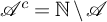
 for which
$\mathscr A^c=\mathbb N\setminus \mathscr A$
for which
$\mathscr A^c=\mathbb N\setminus \mathscr A$
 has positive lower density. Then
$\mathscr A^c$
has positive lower density. Then
$\mathscr A^c$
 is a strongly subconvex
$L^p$
is a strongly subconvex
$L^p$
 -set.
-set.
Proof. The set
$\mathbb N$
 is a strongly subconvex
$L^q$
is a strongly subconvex
$L^q$
 -set whenever
$q>1$
-set whenever
$q>1$
 , and hence also a strongly subconvex
$L^p$
, and hence also a strongly subconvex
$L^p$
 -set. Thus, the conclusion is immediate from Theorem 3.1.
Corollary 3.3. When
$r>s\geqslant 2$
 , the set of r-free numbers that are not s-free, namely
$\mathscr N_r\setminus \mathscr N_s$
, the set of r-free numbers that are not s-free, namely
$\mathscr N_r\setminus \mathscr N_s$
 , is a strongly subconvex
$L^p$
, is a strongly subconvex
$L^p$
 -set whenever
$p>1+1/s$
-set whenever
$p>1+1/s$
 .
.
Proof. As noted in Example 2.2, both
$\mathscr N_r$
 and
$\mathscr N_s$
and
$\mathscr N_s$
 are strongly subconvex
$L^p$
are strongly subconvex
$L^p$
 -sets whenever
$p>1+1/s$
-sets whenever
$p>1+1/s$
 . Since
$\mathscr N_s\subset \mathscr N_r$
. Since
$\mathscr N_s\subset \mathscr N_r$
 and
$\mathscr N_r\setminus \mathscr N_s$
and
$\mathscr N_r\setminus \mathscr N_s$
 has positive density, the desired conclusion follows from Theorem 3.1.
Next, we turn our attention to translations and dilations of sets.
Theorem 3.4. Suppose that
$\mathscr A$
 is a strongly subconvex
$L^p$
is a strongly subconvex
$L^p$
 -set with
$p>1$
-set with
$p>1$
 . Then, whenever
$q\in \mathbb N$
. Then, whenever
$q\in \mathbb N$
 and
$a\in \mathbb Z$
and
$a\in \mathbb Z$
 , the set
$\mathscr B=(q\mathscr A+a)\cap \mathbb N$
, the set
$\mathscr B=(q\mathscr A+a)\cap \mathbb N$
 is also a strongly subconvex
$L^p$
is also a strongly subconvex
$L^p$
 -set.
-set.
Proof. We have

whence, by a change of variable, it follows from (1.1) that

The desired conclusion follows at once.
Perturbations of subconvex
$L^p$
 -sets, in which sufficiently few elements are removed or added, also yield subconvex
$L^p$
-sets, in which sufficiently few elements are removed or added, also yield subconvex
$L^p$
 -sets.
Theorem 3.5. Suppose that
$\mathscr A$
 is a strongly subconvex
$L^p$
is a strongly subconvex
$L^p$
 -set with
$p>1$
-set with
$p>1$
 . Let
$\mathscr B$
. Let
$\mathscr B$
 and
$\mathscr C$
and
$\mathscr C$
 be subsets of
$\mathbb N$
be subsets of
$\mathbb N$
 with
$\mathscr B\subset \mathscr A$
with
$\mathscr B\subset \mathscr A$
 and
$\mathscr C\subset \mathbb N\setminus \mathscr A$
and
$\mathscr C\subset \mathbb N\setminus \mathscr A$
 satisfying the property that

Then the perturbed set
$\mathscr A'=(\mathscr A\setminus \mathscr B)\cup \mathscr C$
 is also a strongly subconvex
$L^p$
is also a strongly subconvex
$L^p$
 -set.
-set.
Proof. One has

whence, it follows from (1.1) that

Since we may assume that
$p<2$
 , it follows from Hölder’s inequality and orthogonality that one has

with a similar upper bound available for the mean value over the exponential sum associated with the set
$\mathscr C(N)$
 . Since
$\mathscr A$
. Since
$\mathscr A$
 is a strongly subconvex
$L^p$
is a strongly subconvex
$L^p$
 -set, it therefore follows from the hypothesis (3.1) that

This confirms that
$\mathscr A'$
 is a strongly subconvex
$L^p$
is a strongly subconvex
$L^p$
 -set.
-set.
A particularly attractive feature of subconvex
$L^p$
 -sets is that intersections of such sets, provided that these intersections remain of positive lower density, are likewise subconvex
$L^q$
-sets is that intersections of such sets, provided that these intersections remain of positive lower density, are likewise subconvex
$L^q$
 -sets, for an appropriate choice of q. The condition here that the intersections have positive lower density is natural. For example, the set
$\mathscr N_2$
-sets, for an appropriate choice of q. The condition here that the intersections have positive lower density is natural. For example, the set
$\mathscr N_2$
 consisting of square-free numbers plainly has the property that
$\mathscr N_2\cap \mathscr N_2^c$
consisting of square-free numbers plainly has the property that
$\mathscr N_2\cap \mathscr N_2^c$
 is empty. So although
$\mathscr N_2$
is empty. So although
$\mathscr N_2$
 and
$\mathscr N_2^c$
and
$\mathscr N_2^c$
 are both weakly subconvex
$L^{3/2}$
are both weakly subconvex
$L^{3/2}$
 -sets, their intersection is not. The problem of determining whether or not two subconvex
$L^p$
-sets, their intersection is not. The problem of determining whether or not two subconvex
$L^p$
 -sets
$\mathscr A$
-sets
$\mathscr A$
 and
$\mathscr B$
and
$\mathscr B$
 have an intersection with positive lower density may have a number-theoretic flavour. In particular, in many examples, the circle method will provide a viable means of establishing whether or not
$\mathscr A\cap \mathscr B$
have an intersection with positive lower density may have a number-theoretic flavour. In particular, in many examples, the circle method will provide a viable means of establishing whether or not
$\mathscr A\cap \mathscr B$
 has positive lower density.
It is convenient in the proof of the next theorem, and elsewhere, to define an exponential sum
$f(\alpha ;\mathscr D)=f_N(\alpha ;\mathscr D)$
 associated with each subset
$\mathscr D$
associated with each subset
$\mathscr D$
 of the natural numbers. Thus, we write

Theorem 3.6. Let
$\mathscr A$
 be a strongly subconvex
$L^q$
be a strongly subconvex
$L^q$
 -set with
$q>1$
-set with
$q>1$
 , and let
$\mathscr B$
, and let
$\mathscr B$
 be a strongly subconvex
$L^r$
be a strongly subconvex
$L^r$
 -set with
$r>1$
-set with
$r>1$
 . Define the real number p via the relation

Suppose in addition that one has

Then the set
$\mathscr A\cup \mathscr B$
 is a strongly subconvex
$L^p$
is a strongly subconvex
$L^p$
 -set, and provided that the set
$\mathscr A\cap \mathscr B$
-set, and provided that the set
$\mathscr A\cap \mathscr B$
 has positive lower density, it is a strongly subconvex
$L^p$
has positive lower density, it is a strongly subconvex
$L^p$
 -set.
-set.
Proof. The desired conclusion concerning
$\mathscr A\cap \mathscr B$
 is essentially a consequence of Young’s convolution inequality (see [Reference Brascamp and Lieb7], for example), though the argument is sufficiently simple and instructive that we take the opportunity to describe our proof in detail. We recall that as a consequence of Definition 1.1, it is implicit that the strong subconvexity of
$\mathscr A$
is essentially a consequence of Young’s convolution inequality (see [Reference Brascamp and Lieb7], for example), though the argument is sufficiently simple and instructive that we take the opportunity to describe our proof in detail. We recall that as a consequence of Definition 1.1, it is implicit that the strong subconvexity of
$\mathscr A$
 and
$\mathscr B$
and
$\mathscr B$
 implies that
$q<2$
implies that
$q<2$
 and
$r<2$
and
$r<2$
 . Define the real number p via the relation (3.3), and note that the condition (3.4) then ensures that
$1<p<2$
. Define the real number p via the relation (3.3), and note that the condition (3.4) then ensures that
$1<p<2$
 . Also, put
$\mathscr C=\mathscr A\cap \mathscr B$
. Also, put
$\mathscr C=\mathscr A\cap \mathscr B$
 . Then on making use of the notation (3.2), it follows from orthogonality that one has

Next, observe that as a consequence of the last relation, it follows from (1.1) that

An application of Hölder’s inequality therefore reveals that

where

Here, we have made use of the observation that

so that
$0<1/q-1/p<1$
 , and similarly
$0<1/r-1/p<1$
, and similarly
$0<1/r-1/p<1$
 . Moreover,

Hence, our application of Hölder’s inequality is legitimate.
By applying a change of variables, and utilising the definition (1.1) and the fact that
$\mathscr A$
 is a strongly subconvex
$L^q$
is a strongly subconvex
$L^q$
 -set, we find that

Similarly, one sees that
$T_2\ll N^{r-1}I_p(N;\mathscr C)$
 , and
, and

We therefore deduce from (3.5) that

Our hypothesis that the set
$\mathscr C=\mathscr A\cap \mathscr B$
 has positive lower density ensures that when
$0\leqslant \alpha \leqslant (100N)^{-1}$
has positive lower density ensures that when
$0\leqslant \alpha \leqslant (100N)^{-1}$
 , one has

whence

Then we conclude from (3.6) that
$I_p(N;\mathscr C)^{1/p}\ll N^{1-1/p}$
 , whence
$I_p(N;\mathscr C)\ll N^{p-1}$
, whence
$I_p(N;\mathscr C)\ll N^{p-1}$
 . This confirms that
$\mathscr A\cap \mathscr B$
. This confirms that
$\mathscr A\cap \mathscr B$
 is a strongly subconvex
$L^p$
is a strongly subconvex
$L^p$
 -set.
-set.
The conclusion concerning
$\mathscr A\cup \mathscr B$
 follows by observing that

Since our work on the case
$\mathscr A\cap \mathscr B$
 shows that the p-th moment of each of the exponential sums on the right hand side is
$O(N^{p-1})$
shows that the p-th moment of each of the exponential sums on the right hand side is
$O(N^{p-1})$
 , the desired conclusion
$I_p(N;\mathscr A\cup \mathscr B)\ll N^{p-1}$
, the desired conclusion
$I_p(N;\mathscr A\cup \mathscr B)\ll N^{p-1}$
 is immediate.
This conclusion yields an immediate corollary for intersections of subconvex
$L^p$
 -sets with Beatty sequences.
Corollary 3.7. Let
$\mathscr A$
 be a strongly subconvex
$L^q$
be a strongly subconvex
$L^q$
 -set for some real number
$q\in (1,2)$
-set for some real number
$q\in (1,2)$
 . Suppose that
$\alpha $
. Suppose that
$\alpha $
 and
$\beta $
and
$\beta $
 are real numbers with
$\alpha>0$
are real numbers with
$\alpha>0$
 such that
$1/\alpha $
such that
$1/\alpha $
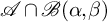
 is of finite Diophantine type. Then the set
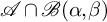
$\mathscr A\cap \mathscr B(\alpha ,\beta )$
is of finite Diophantine type. Then the set
$\mathscr A\cap \mathscr B(\alpha ,\beta )$
 is a strongly subconvex
$L^p$
is a strongly subconvex
$L^p$
 -set whenever p is a real number with
$p\in (q,2)$
-set whenever p is a real number with
$p\in (q,2)$
 and
$\mathscr A\cap \mathscr B(\alpha ,\beta )$
and
$\mathscr A\cap \mathscr B(\alpha ,\beta )$
 has positive lower density.
Proof. The Beatty sequence
$\mathscr B(\alpha ,\beta )$
 is a strongly subconvex
$L^r$
is a strongly subconvex
$L^r$
 -set whenever
$1<r<2$
-set whenever
$1<r<2$
 , as a consequence of Theorem 2.3. Choose any such value of r sufficiently close to
$1$
, as a consequence of Theorem 2.3. Choose any such value of r sufficiently close to
$1$
 , and define the real number p by means of the relation (3.3). Then we may take p as close as we like to q by choosing r suitably close to
$1$
, and define the real number p by means of the relation (3.3). Then we may take p as close as we like to q by choosing r suitably close to
$1$
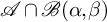
 . The conclusion of Theorem 3.6 then shows that
$\mathscr A\cap \mathscr B(\alpha ,\beta )$
. The conclusion of Theorem 3.6 then shows that
$\mathscr A\cap \mathscr B(\alpha ,\beta )$
 is a strongly subconvex
$L^p$
is a strongly subconvex
$L^p$
 -set provided that this set has positive lower density and condition (3.4) is satisfied. Since
$q>1$
-set provided that this set has positive lower density and condition (3.4) is satisfied. Since
$q>1$
 and
$r>1$
and
$r>1$
 , the upper bound on
$1/q+1/r$
, the upper bound on
$1/q+1/r$
 in the latter condition is automatically satisfied. Moreover, one has
$q<2$
in the latter condition is automatically satisfied. Moreover, one has
$q<2$
 , so the lower bound
$1/q+1/r>3/2$
, so the lower bound
$1/q+1/r>3/2$
 is satisfied on taking r sufficiently close to
$1$
is satisfied on taking r sufficiently close to
$1$
 . The desired conclusion therefore follows.
The discussion of this section exhibits numerous means of generating new examples of subconvex
$L^p$
 -sets from any existing examples. One can also splice together different sets by considering (in the obvious sense) such hybrid examples as

when given subconvex
$L^p$
 -sets
$\mathscr A$
-sets
$\mathscr A$
 ,
$\mathscr B$
,
$\mathscr B$
 and
$\mathscr C$
and
$\mathscr C$
 . A basic problem worthy of attention would be to characterise subconvex
$L^p$
. A basic problem worthy of attention would be to characterise subconvex
$L^p$
 -sets.
Problem 3.8. Suppose that p is a real number with
$1<p<2$
 . Characterise, to the extent possible, strongly subconvex
$L^p$
. Characterise, to the extent possible, strongly subconvex
$L^p$
 -sets.
4 Weyl sums over weakly subconvex
$L^p$
-sets, I

We begin with the most striking of the applications of subconvex
$L^p$
 -sets to exponential sums over polynomials having summands restricted to these
$L^p$
-sets to exponential sums over polynomials having summands restricted to these
$L^p$
 -sets, demonstrating how to establish the upper bound (1.9) of Theorem 1.2.
Proof of Theorem 1.2.
Let
$\mathscr A$
 be a weakly subconvex
$L^p$
be a weakly subconvex
$L^p$
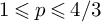
 -set for some real number p with
$1\leqslant p\leqslant 4/3$
-set for some real number p with
$1\leqslant p\leqslant 4/3$
 . We may suppose that
$k\geqslant 3$
. We may suppose that
$k\geqslant 3$
 , and that
$a\in \mathbb Z$
, and that
$a\in \mathbb Z$
 and
$q\in \mathbb N$
and
$q\in \mathbb N$
 satisfy
$(a,q)=1$
satisfy
$(a,q)=1$
 and
$|\alpha _k-a/q|\leqslant q^{-2}$
and
$|\alpha _k-a/q|\leqslant q^{-2}$
 . We recall the definition (1.6), and introduce the exponential sum
$F_k(\boldsymbol \alpha )=F_k(\boldsymbol \alpha ;N)$
. We recall the definition (1.6), and introduce the exponential sum
$F_k(\boldsymbol \alpha )=F_k(\boldsymbol \alpha ;N)$
 , defined by

We also make use of the exponential sum
$g(\alpha )=f_N(\alpha ;\mathscr A)$
 defined via (3.2), so that

and introduce the exponential sum

We note that
$G_k(\boldsymbol \alpha ,\beta )$
 is merely a more convenient form of an exponential sum that may be written in terms of the sum
$\Psi _k(\boldsymbol \alpha ;N)$
is merely a more convenient form of an exponential sum that may be written in terms of the sum
$\Psi _k(\boldsymbol \alpha ;N)$
 defined in (1.7). It now follows from orthogonality that one has the fundamental relation

An application of Hölder’s inequality reveals that

Here, our hypothesis that
$\mathscr A$
 is a weakly subconvex
$L^p$
is a weakly subconvex
$L^p$
 -set for some real number p with
$p\leqslant 4/3$
-set for some real number p with
$p\leqslant 4/3$
 ensures that

Hence, we deduce from (4.5) that

By orthogonality, the integral on the right hand side of (4.6) may be interpreted in the form

For suitable integers
$h_1$
 and
$h_2$
and
$h_2$
 with
$|h_i|<N\, (i=1,2)$
with
$|h_i|<N\, (i=1,2)$
 , one can write the summands
$n_3$
, one can write the summands
$n_3$
 and
$n_4$
and
$n_4$
 in the shape

The relation
$n_1+n_2=n_3+n_4$
 then implies that
$n_2=n_1+h_1+h_2$
then implies that
$n_2=n_1+h_1+h_2$
 . Thus, making use of the forward difference operator

and the second order operator

we see that

In this way, we conclude that

in which
$\mathscr I(N;{\mathbf h})$
 denotes the interval of integers defined by

The right hand side of (4.7) will be recognised as the principal output of a second order Weyl differencing process applied to the exponential sum
$G_k(\boldsymbol \alpha ,0)=\Psi _k(\boldsymbol \alpha ;N)$
 . The interested reader should direct their attention to [Reference Vaughan24, Lemma 2.3] and compare with the situation therein with
$j=2$
. The interested reader should direct their attention to [Reference Vaughan24, Lemma 2.3] and compare with the situation therein with
$j=2$
 .
.
On substituting (4.7) into (4.6), we see that

where

in which
$\mathscr I_2=\mathscr I(N;{\mathbf h})$
 . A comparison of this upper bound with the statement of [Reference Vaughan24, Lemma 2.3] reveals, just as in the proof of [Reference Vaughan24, Lemma 2.4], that the application of
$k-3$
. A comparison of this upper bound with the statement of [Reference Vaughan24, Lemma 2.3] reveals, just as in the proof of [Reference Vaughan24, Lemma 2.4], that the application of
$k-3$
 further Weyl differencing steps delivers the bound

where
$\mathscr I_{k-1}$
 is a subinterval of integers lying within
$[1,N]$
is a subinterval of integers lying within
$[1,N]$
 , and
, and

Hence, just as in the completion of the argument of the proof of [Reference Vaughan24, Lemma 2.4], one concludes that

Thus

confirming the desired conclusion (1.9).
We next address the proof of Theorem 1.3. This we achieve in two stages, the second of which we defer to the next section. We recall the definition of the exponent
$\sigma _p(k)$
 recorded in the preamble to the statement of Theorem 1.3.
Lemma 4.1. Suppose that
$\mathscr A$
 is a weakly subconvex
$L^p$
is a weakly subconvex
$L^p$
 -set for some real number p with
$1\leqslant p<2$
-set for some real number p with
$1\leqslant p<2$
 , and further that
$k\geqslant 2$
, and further that
$k\geqslant 2$
 . Let
$(\alpha _0,\alpha _1,\ldots ,\alpha _k)\in \mathbb R^{k+1}$
. Let
$(\alpha _0,\alpha _1,\ldots ,\alpha _k)\in \mathbb R^{k+1}$
 , and suppose that
$a\in \mathbb Z$
, and suppose that
$a\in \mathbb Z$
 and
$q\in \mathbb N$
and
$q\in \mathbb N$
 satisfy
$(a,q)=1$
satisfy
$(a,q)=1$
 and
$|\alpha _k-a/q|\leqslant q^{-2}$
and
$|\alpha _k-a/q|\leqslant q^{-2}$
 . Then, for each
$\varepsilon>0$
. Then, for each
$\varepsilon>0$
 and each large real number N, one has

Proof. We begin by noting that when
$\mathscr A$
 is a weakly subconvex
$L^1$
is a weakly subconvex
$L^1$
 -set, then it is also a weakly subconvex
$L^p$
-set, then it is also a weakly subconvex
$L^p$
 -set for any
$p>1$
-set for any
$p>1$
 . The conclusion of Theorem 1.3 for
$p=1$
. The conclusion of Theorem 1.3 for
$p=1$
 is obtained from that for
$1<p<2$
is obtained from that for
$1<p<2$
 by taking p sufficiently close to
$1$
by taking p sufficiently close to
$1$
 , on adjusting the value of
$\varepsilon $
, on adjusting the value of
$\varepsilon $
 in the desired conclusion. There is consequently no loss of generality in supposing throughout that
$1<p<2$
in the desired conclusion. There is consequently no loss of generality in supposing throughout that
$1<p<2$
 and
$k\geqslant 2$
and
$k\geqslant 2$
 . Next, we observe that in the case
$k=2$
. Next, we observe that in the case
$k=2$
 it makes little sense to perform two Weyl differencing steps, so that the proof of Theorem 1.2 is of limited use to us. In this case we nonetheless have the orthogonality relation (4.4), but in present circumstances we apply Hölder’s inequality to obtain the upper bound

Our hypothesis that
$\mathcal A$
 is a weakly subconvex
$L^p$
is a weakly subconvex
$L^p$
 -set ensures via (1.2) that

Moreover, since
$1<p<2$
 , we may suppose that
$p/(p-1)>2$
, we may suppose that
$p/(p-1)>2$
 . Hence, by orthogonality, we see that

Since
$a\in \mathbb Z$
 and
$q\in \mathbb N$
and
$q\in \mathbb N$
 satisfy
$(a,q)=1$
satisfy
$(a,q)=1$
 and
$|\alpha _k-a/q|\leqslant q^{-2}$
and
$|\alpha _k-a/q|\leqslant q^{-2}$
 , it follows from Weyl’s inequality (see [Reference Vaughan24, Lemma 2.4]) that we have the bound

Thus we see from (4.11) that

On substituting this estimate together with (4.10) into (4.9), we conclude that

Thus far, our discussion has been independent of the value of
$k\geqslant 2$
 . Specialising to the situation with
$k=2$
. Specialising to the situation with
$k=2$
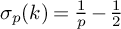
 , however, we obtain the estimate (4.8) with
$\sigma _p(k)=\frac {1}{p}-\frac {1}{2}$
, however, we obtain the estimate (4.8) with
$\sigma _p(k)=\frac {1}{p}-\frac {1}{2}$
 , confirming the conclusion of the lemma in this case.
The situation with
$k\geqslant 3$
 and
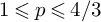
$1\leqslant p\leqslant 4/3$
and
$1\leqslant p\leqslant 4/3$
 is immediate from Theorem 1.2, since, in such circumstances, one has
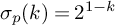
$\sigma _p(k)=2^{1-k}$
is immediate from Theorem 1.2, since, in such circumstances, one has
$\sigma _p(k)=2^{1-k}$
 . We turn now to address the situation in which
$k\geqslant 3$
. We turn now to address the situation in which
$k\geqslant 3$
 and
$4/3<p<2$
and
$4/3<p<2$
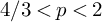 . Here, our starting point is the relation (4.4), though we apply Hölder’s inequality in a manner that incorporates the
$4$
. Here, our starting point is the relation (4.4), though we apply Hölder’s inequality in a manner that incorporates the
$4$
 -th moment of
$G_k(\boldsymbol \alpha ,\beta )$
-th moment of
$G_k(\boldsymbol \alpha ,\beta )$
 . Thus, we obtain

where

By orthogonality, one finds from (4.3) that
$U_1\leqslant N$
 . Meanwhile, the argument leading from (4.7) to the conclusion of the proof of Theorem 1.2 shows that

Thus, on recalling the upper bound (4.10), we deduce from (4.12) that

Since
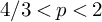
$\sigma _p(k)=\big ( \frac {1}{p}-\frac {1}{2}\big )2^{3-k}$
 when
$k\geqslant 3$
when
$k\geqslant 3$
 and
$4/3<p<2$
and
$4/3<p<2$
 , this confirms the conclusion of the lemma in this final case.
5 Weyl sums over weakly subconvex
$L^p$
-sets, II

We next shift attention to the application of Vinogradov’s methods for bounding exponential sums, though now with the variables restricted to subconvex
$L^p$
 -sets. Here, we adopt an approach that differs from that more familiarly presented in work, for example, of Vaughan [Reference Vaughan24, §5.2].
Lemma 5.1. Suppose that
$\mathscr A$
 is a weakly subconvex
$L^p$
is a weakly subconvex
$L^p$
 -set for some real number p with
$1\leqslant p<2$
-set for some real number p with
$1\leqslant p<2$
 , and further that
$k\geqslant 3$
, and further that
$k\geqslant 3$
 . Let
$(\alpha _0,\alpha _1,\ldots ,\alpha _k)\in \mathbb R^{k+1}$
. Let
$(\alpha _0,\alpha _1,\ldots ,\alpha _k)\in \mathbb R^{k+1}$
 , and suppose that
$a\in \mathbb Z$
, and suppose that
$a\in \mathbb Z$
 and
$q\in \mathbb N$
and
$q\in \mathbb N$
 satisfy
$(a,q)=1$
satisfy
$(a,q)=1$
 and
$|\alpha _k-a/q|\leqslant q^{-2}$
and
$|\alpha _k-a/q|\leqslant q^{-2}$
 . Then, for each
$\varepsilon>0$
. Then, for each
$\varepsilon>0$
 and each large real number N, one has

Proof. Just as in the proof of Lemma 4.1, there is no loss of generality in supposing throughout that
$1<p<2$
 . Furthermore, in view of the definition of
$\tau _p(k)$
. Furthermore, in view of the definition of
$\tau _p(k)$
 , we may suppose in addition that
$k\geqslant 3$
, we may suppose in addition that
$k\geqslant 3$
 . Moreover, we again have the upper bounds (4.9) and (4.10) employed in the course of the proof of Lemma 4.1. We augment these estimates with a new mean value estimate. Write

It transpires that we are able to bound
$|F_k(\boldsymbol \alpha )|$
 in terms of the mean value
$U_r$
in terms of the mean value
$U_r$
 , defined as in (4.13). It is this mean value to which we apply Vinogradov’s methods.
Observe first that from (4.3), one has

Thus, by Hölder’s inequality, one sees that

in which we write

Next, write

and put

Then we see via orthogonality that

where we abbreviate
$\beta _2m_2+\ldots +\beta _{k-2}m_{k-2}$
 to
$\boldsymbol \beta \cdot {\mathbf m}$
to
$\boldsymbol \beta \cdot {\mathbf m}$
 . An application of the triangle inequality therefore propels us from (5.3) to the bound

By orthogonality, the mean value on the right hand side of (5.4) is equal to

in which we write

and the summation over
$h_1,\ldots ,h_{2r}$
 is subject to the condition

By expanding the polynomial
$\psi (n+h;\boldsymbol \alpha )$
 using the binomial theorem, moreover, we see that for each summand
${\mathbf h}$
using the binomial theorem, moreover, we see that for each summand
${\mathbf h}$
 , we have

Hence, with the same implicit condition on
$h_1,\ldots ,h_{2r}$
 , we deduce that

where
$\mathscr I({\mathbf h})$
 denotes the set of integers n in the interval
$[1,N]$
denotes the set of integers n in the interval
$[1,N]$
 satisfying the property that

Since the set
$\mathscr I({\mathbf h})$
 is a subinterval of the integers lying in
$[1,N]$
is a subinterval of the integers lying in
$[1,N]$
 , it follows in a standard manner that by summing the implicit geometric progression, one has

By substituting this bound into (5.5), and thence into (5.4), we conclude thus far that

where we write
$\rho (m)$
 for the number of solutions of the system of equations

with
$|h_i|\leqslant N\, (1\leqslant i\leqslant 2r)$
 .
.
A standard application of the recent resolution of the main conjecture on Vinogradov’s mean value theorem (see [Reference Bourgain, Demeter and Guth6], [Reference Wooley28], [Reference Wooley29]) shows via orthogonality that

Thus, we infer from (5.2) and (5.6) that

A standard reciprocal sums lemma (see, for example, [Reference Vaughan24, Lemma 2.2]) leads from here to the estimate

We may now return to combine (5.7) with the bounds (4.9) and (4.10) already established. Observe first that when
$p/(p-1)=2r$
 , which is to say that
$p=2r/(2r-1)$
, which is to say that
$p=2r/(2r-1)$
 , the estimate (5.7) may be substituted into (4.9) along with (4.10) to give

Since any weakly subconvex
$L^q$
 -set with
$q<2r/(2r-1)$
-set with
$q<2r/(2r-1)$
 is also a weakly subconvex
$L^p$
is also a weakly subconvex
$L^p$
 -set with
$p=2r/(2r-1)$
-set with
$p=2r/(2r-1)$
 , and
, and

this establishes (5.1) when
$k\geqslant 3$
 and
$1\leqslant p\leqslant 1+1/(k^2-k-1)$
and
$1\leqslant p\leqslant 1+1/(k^2-k-1)$
 .
.
The situation with
$1+1/(k^2-k-1)<p<2$
 requires more care. Applying Hölder’s inequality to (4.4), we obtain the upper bound

where
$U_1$
 and
$U_r$
and
$U_r$
 are defined as in (4.13), and

Notice here that since

one has

It follows that
$\omega _r<1-1/p$
 , whence our application of Hölder’s inequality was indeed legitimate.
The bound
$U_1\leqslant N$
 again follows via orthogonality, while the bound (5.7) supplies an estimate for
$U_r$
again follows via orthogonality, while the bound (5.7) supplies an estimate for
$U_r$
 . Consequently, on substituting these estimates along with (4.10) into (5.8), we deduce that

Since
$\tau _p(k)=\omega _r$
 in present circumstances, this completes the proof of the lemma.
The proof of Theorem 1.3 is completed by combining the conclusions of Lemmata 4.1 and 5.1. The former addresses the situations with
$k\geqslant 2$
 when
$\sigma _p(k)\geqslant \tau _p(k)$
when
$\sigma _p(k)\geqslant \tau _p(k)$
 , and the latter addresses those scenarios in which
$k\geqslant 3$
, and the latter addresses those scenarios in which
$k\geqslant 3$
 and
$\tau _p(k)\geqslant \sigma _p(k)$
and
$\tau _p(k)\geqslant \sigma _p(k)$
 .
.
Enthusiastic readers might choose to entertain themselves by adapting these methods to show that when
$k\geqslant 6$
 and
$1\leqslant p\leqslant 4/3$
and
$1\leqslant p\leqslant 4/3$
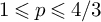 , one has an analogue of Heath-Brown’s refinement of Weyl’s inequality for weakly subconvex
$L^p$
, one has an analogue of Heath-Brown’s refinement of Weyl’s inequality for weakly subconvex
$L^p$
 -sets
$\mathscr A$
-sets
$\mathscr A$
 . Thus, when
$\alpha \in \mathbb R$
. Thus, when
$\alpha \in \mathbb R$
 , and
$a\in \mathbb Z$
, and
$a\in \mathbb Z$
 and
$q\in \mathbb N$
and
$q\in \mathbb N$
 satisfy
$(a,q)=1$
satisfy
$(a,q)=1$
 and
$|\alpha -a/q|\leqslant q^{-2}$
and
$|\alpha -a/q|\leqslant q^{-2}$
 , one may adapt the proof of [Reference Heath-Brown12, Theorem 1] to show that

6 Equidistribution and subconvex
$L^p$
-sets

In order to explore the topic of equidistribution of polynomial sequences with arguments from subconvex
$L^p$
 -sets, we apply Weyl’s criterion. Recall that the sequence
$(a_n)_{n=1}^\infty $
-sets, we apply Weyl’s criterion. Recall that the sequence
$(a_n)_{n=1}^\infty $
 is equidistributed modulo
$1$
is equidistributed modulo
$1$
 if and only if for any integer
$m\ne 0$
if and only if for any integer
$m\ne 0$
 , we have

Define the polynomial
$\psi (x;\boldsymbol \alpha )$
 as in (1.6) with fixed coefficients
$\boldsymbol \alpha \in \mathbb R^{k+1}$
as in (1.6) with fixed coefficients
$\boldsymbol \alpha \in \mathbb R^{k+1}$
 . Then as a particular consequence of work of Weyl [Reference Weyl26], the sequence
$(\psi (n;\boldsymbol \alpha ))_{n=1}^\infty $
. Then as a particular consequence of work of Weyl [Reference Weyl26], the sequence
$(\psi (n;\boldsymbol \alpha ))_{n=1}^\infty $
 is equidistributed modulo
$1$
is equidistributed modulo
$1$
 whenever one at least of the coefficients
$\alpha _2,\ldots ,\alpha _k$
whenever one at least of the coefficients
$\alpha _2,\ldots ,\alpha _k$
 is irrational. In these circumstances, we see that for each non-zero integer m, one has

Our objective in this section is to establish an analogue of this last conclusion in which the summands n are restricted to a subconvex
$L^p$
 -set. We begin with the proof of Theorem 1.4, which concerns strongly subconvex
$L^p$
-set. We begin with the proof of Theorem 1.4, which concerns strongly subconvex
$L^p$
 -sets.
Proof of Theorem 1.4.
Let
$\mathscr A=\{a_1,a_2,\ldots \}$
 , with
$a_1<a_2<\ldots $
, with
$a_1<a_2<\ldots $
 , be a strongly subconvex
$L^p$
, be a strongly subconvex
$L^p$
 -set with
$1\leqslant p<2$
-set with
$1\leqslant p<2$
 . In order to facilitate tidier notation, we make a modest preliminary manoeuvre. Since
$\mathscr A$
. In order to facilitate tidier notation, we make a modest preliminary manoeuvre. Since
$\mathscr A$
 has positive lower density in
$\mathbb N$
has positive lower density in
$\mathbb N$
 , we see that there exists a positive number
$c=c(\mathscr A)$
, we see that there exists a positive number
$c=c(\mathscr A)$
 having the property that when M is large, there exists an integer N with
$N\leqslant cM$
having the property that when M is large, there exists an integer N with
$N\leqslant cM$
 for which one has
$\{a_1,a_2,\ldots ,a_M\}=\mathscr A(N)$
for which one has
$\{a_1,a_2,\ldots ,a_M\}=\mathscr A(N)$
 . Next, let
$k\geqslant 2$
. Next, let
$k\geqslant 2$
 , and define
$\psi (n;\boldsymbol \alpha )$
, and define
$\psi (n;\boldsymbol \alpha )$
 according to (1.6). The hypotheses of the theorem permit us the assumption that one at least of the coefficients
$\alpha _2,\ldots ,\alpha _k$
according to (1.6). The hypotheses of the theorem permit us the assumption that one at least of the coefficients
$\alpha _2,\ldots ,\alpha _k$
 is irrational. We may therefore suppose that there is an integer h with
$2\leqslant h\leqslant k$
is irrational. We may therefore suppose that there is an integer h with
$2\leqslant h\leqslant k$
 for which
$\alpha _k,\ldots ,\alpha _{h+1}$
for which
$\alpha _k,\ldots ,\alpha _{h+1}$
 are all rational, and
$\alpha _h$
are all rational, and
$\alpha _h$
 is irrational. We may suppose in addition that r is a natural number having the property that
$r\alpha _j\in \mathbb Z\ (h+1\leqslant j\leqslant k)$
is irrational. We may suppose in addition that r is a natural number having the property that
$r\alpha _j\in \mathbb Z\ (h+1\leqslant j\leqslant k)$
 . In this context, if
$h=k$
. In this context, if
$h=k$
 , then we set
$r=1$
, then we set
$r=1$
 .
.
According to Weyl’s criterion, the sequence
$(\psi (a_n;\boldsymbol \alpha ))_{n=1}^\infty $
 is equidistributed modulo
$1$
is equidistributed modulo
$1$
 if and only if for any integer
$m\ne 0$
if and only if for any integer
$m\ne 0$
 , one has

The latter holds if and only if

Thus, in the notation introduced in (4.1), our goal is to show that for any integer
$m\ne 0$
 , one has

Applying the notation (4.2) and (4.3) employed in the course of the proof of Theorem 1.2, we may infer from (4.4) that

An application of Hölder’s inequality reveals that

Since
$\mathscr A$
 is a strongly subconvex
$L^p$
is a strongly subconvex
$L^p$
 -set with
$1\leqslant p<2$
-set with
$1\leqslant p<2$
 , we have

Then it follows via orthogonality that

Thus, we may infer that the estimate (6.1) holds whenever one has

We establish (6.3) in a fairly routine manner via a sequence of intermediate steps. We begin by considering an auxiliary polynomial

and the associated exponential sum

Suppose that
$\beta _h$
 is irrational. We claim that for any fixed value of
$\eta>1$
is irrational. We claim that for any fixed value of
$\eta>1$
 , there exists a natural number
$N_0$
, there exists a natural number
$N_0$
 having the property that

We establish this claim by contradiction. Suppose, if possible, that for all large values of N, one has

Then it follows from an appropriate version of Weyl’s inequality (see [Reference Baker2, Theorem 5.1]) that there exist
$a\in \mathbb Z$
 and
$q\in \mathbb N$
and
$q\in \mathbb N$
 with
$(a,q)=1$
with
$(a,q)=1$
 ,
,

For each large natural number Q, we fix
$N=\lfloor (Q/\eta ^h)^3\rfloor $
 . Then we find that one has
$q<Q$
. Then we find that one has
$q<Q$
 and
$|q\beta _h-a|<Q^{-3/2}$
and
$|q\beta _h-a|<Q^{-3/2}$
 . Since these inequalities hold for all large values of Q, it follows via a consideration of the continued fraction convergents to
$\beta _h$
. Since these inequalities hold for all large values of Q, it follows via a consideration of the continued fraction convergents to
$\beta _h$
 that this coefficient must be rational (compare [Reference Lê, Liu and Wooley19, Lemma 2.7]). This deduction contradicts our assumption that
$\beta _h$
that this coefficient must be rational (compare [Reference Lê, Liu and Wooley19, Lemma 2.7]). This deduction contradicts our assumption that
$\beta _h$
 is irrational, and so we are forced to conclude that our claim (6.4) is indeed valid.
Now we return to consider the exponential sum
$G_k(m\boldsymbol \alpha ,\beta )$
 and the bound (6.3) that we seek to establish. Let
$\eta>1$
and the bound (6.3) that we seek to establish. Let
$\eta>1$
 be arbitrary. Put
$\beta _h=mr^h\alpha _h$
be arbitrary. Put
$\beta _h=mr^h\alpha _h$
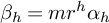 . Then since one has
$r\alpha _j\in \mathbb Z (h+1\leqslant j\leqslant k)$
. Then since one has
$r\alpha _j\in \mathbb Z (h+1\leqslant j\leqslant k)$
 , we see that

for some real numbers
$\beta _0,\ldots ,\beta _{h-1}$
 depending at most on r, m, x,
$\beta $
depending at most on r, m, x,
$\beta $
 and
$\boldsymbol \alpha $
and
$\boldsymbol \alpha $
 . Notice that since
$\alpha _h$
. Notice that since
$\alpha _h$
 is presumed to be irrational, so too is
$\beta _h$
is presumed to be irrational, so too is
$\beta _h$
 . Let
$N_0$
. Let
$N_0$
 be the natural number furnished in association with the upper bound (6.4) that we have established. When N is large enough in terms of r and
$N_0$
be the natural number furnished in association with the upper bound (6.4) that we have established. When N is large enough in terms of r and
$N_0$
 , one has

Then we deduce from (6.4) that

Therefore, for each integer
$m\ne 0$
 , we conclude that for every real number
$\eta>1$
, we conclude that for every real number
$\eta>1$
 , one has

Since this upper bound holds for all
$\eta>1$
 , we infer that

and the desired conclusion (6.3) follows. We therefore conclude that (6.1) holds, and so the sequence
$(\psi (a_n;\boldsymbol \alpha ))_{n=1}^\infty $
 is equidistributed modulo
$1$
is equidistributed modulo
$1$
 . This completes the proof of the theorem.
The reader might well be puzzled that the conclusion of Theorem 1.4 applies only to polynomials of the shape
$\psi (t;\boldsymbol \alpha )=\alpha _kt^k+\ldots +\alpha _1t+\alpha _0$
 when one at least of
$\alpha _2,\ldots , \alpha _k$
when one at least of
$\alpha _2,\ldots , \alpha _k$
 is irrational. It transpires that this condition is essential. Were it to be the case that
$\alpha _2,\ldots ,\alpha _k$
is irrational. It transpires that this condition is essential. Were it to be the case that
$\alpha _2,\ldots ,\alpha _k$
 are rational and
$\alpha _1$
are rational and
$\alpha _1$
 is irrational, then it is possible that the sequence
$(\psi (a_n;\boldsymbol \alpha ))_{n=1}^\infty $
is irrational, then it is possible that the sequence
$(\psi (a_n;\boldsymbol \alpha ))_{n=1}^\infty $
 is not equidistributed modulo
$1$
is not equidistributed modulo
$1$
 . Consider, for example, an irrational number
$\theta \in (0,1)$
. Consider, for example, an irrational number
$\theta \in (0,1)$
 of finite Diophantine type and the set

On the one hand, this Beatty sequence
$\{a_1,a_2,\ldots \}$
 , with
$a_1<a_2<\ldots $
, with
$a_1<a_2<\ldots $
 , has the property that
$\{ a_n\theta \}\in (1-\theta ,1)$
, has the property that
$\{ a_n\theta \}\in (1-\theta ,1)$
 for each
$n\in \mathbb N$
for each
$n\in \mathbb N$
 . It is therefore not possible that the sequence
$(a_n\theta )_{n=1}^\infty $
. It is therefore not possible that the sequence
$(a_n\theta )_{n=1}^\infty $
 is equidistributed modulo
$1$
is equidistributed modulo
$1$
 . On the other hand, as a consequence of Theorem 2.3, we see that
$\mathscr A$
. On the other hand, as a consequence of Theorem 2.3, we see that
$\mathscr A$
 is a strongly subconvex
$L^p$
is a strongly subconvex
$L^p$
 -set whenever
$p>1$
-set whenever
$p>1$
 . A modest adjustment of this argument would deliver the same conclusion for the polynomial
$\alpha _kt^k+\ldots +\alpha _1t+\alpha _0$
. A modest adjustment of this argument would deliver the same conclusion for the polynomial
$\alpha _kt^k+\ldots +\alpha _1t+\alpha _0$
 when
$\alpha _k,\ldots ,\alpha _2$
when
$\alpha _k,\ldots ,\alpha _2$
 are all rational and
$\alpha _1=\theta $
are all rational and
$\alpha _1=\theta $
 .
.
We finish this section by noting that a conclusion similar to Theorem 1.4 may be established in which the sequence
$\mathscr A$
 is assumed only to be a weakly subconvex
$L^p$
is assumed only to be a weakly subconvex
$L^p$
 -set with
$1\leqslant p<2$
-set with
$1\leqslant p<2$
 .
.
Theorem 6.1. Suppose that
$\mathscr A=\{a_1,a_2,\ldots \}$
 , with
$a_1<a_2<\ldots $
, with
$a_1<a_2<\ldots $
 , is a weakly subconvex
$L^p$
, is a weakly subconvex
$L^p$
 -set with
$1\leqslant p<2$
-set with
$1\leqslant p<2$
 . Let
$k\geqslant 2$
. Let
$k\geqslant 2$
 , suppose that
$(\alpha _0,\alpha _1,\ldots ,\alpha _k)\in \mathbb R^{k+1}$
, suppose that
$(\alpha _0,\alpha _1,\ldots ,\alpha _k)\in \mathbb R^{k+1}$
 , and define the polynomial
$\psi (x;\boldsymbol \alpha )$
, and define the polynomial
$\psi (x;\boldsymbol \alpha )$
 as in (1.6). Suppose in addition that one at least of the coefficients
$\alpha _2,\ldots ,\alpha _k$
as in (1.6). Suppose in addition that one at least of the coefficients
$\alpha _2,\ldots ,\alpha _k$
 is of finite Diophantine type. Then the sequence
$(\psi (a_n;\boldsymbol \alpha ))_{n=1}^\infty $
is of finite Diophantine type. Then the sequence
$(\psi (a_n;\boldsymbol \alpha ))_{n=1}^\infty $
 is equidistributed modulo
$1$
is equidistributed modulo
$1$
 .
.
Proof. We may proceed just as in the proof of Theorem 1.4, though the hypothesis that
$\mathscr A$
 be weakly subconvex instead of strongly subconvex requires us to replace (6.2) by the bound

Let
$\varepsilon $
 be a small positive number. Then it follows from Baker [Reference Baker2, Theorem 5.1] that whenever
$P>N^{1-2^{-k}}$
be a small positive number. Then it follows from Baker [Reference Baker2, Theorem 5.1] that whenever
$P>N^{1-2^{-k}}$
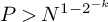 and
$|G_k(m\boldsymbol \alpha ,\beta )|>P$
and
$|G_k(m\boldsymbol \alpha ,\beta )|>P$
 , then there exist
$q\in \mathbb N$
, then there exist
$q\in \mathbb N$
 and
$a_1,\ldots ,a_k\in \mathbb Z$
and
$a_1,\ldots ,a_k\in \mathbb Z$
 having the property that


and

We may suppose that there is an index l with
$2\leqslant l\leqslant k$
 for which
$\alpha _l$
for which
$\alpha _l$
 is of finite Diophantine type. Thus, for some natural number r and positive number c, it follows that for all
$a\in \mathbb Z$
is of finite Diophantine type. Thus, for some natural number r and positive number c, it follows that for all
$a\in \mathbb Z$
 one has

We take

Then we deduce from the above discussion that whenever

there exist
$q\in \mathbb N$
 and
$a\in \mathbb Z$
and
$a\in \mathbb Z$
 with
with

and

But then we find from (6.6) that

whence for large enough values of N, one sees that
$q>N^{1/r}$
 . Thus, we deduce that

leading to a contradiction. We must therefore conclude that whenever N is sufficiently large in terms of m and
$\alpha _l$
 , one has

uniformly in
$\beta $
 . We thus deduce from (6.5) that

whence, for each integer
$m\ne 0$
 , one has

This shows that

so that
$(\psi (a_n;\boldsymbol \alpha ))_{n=1}^\infty $
 is equidistributed modulo
$1$
is equidistributed modulo
$1$
 . This completes the proof of the theorem.
7 Subconvex
$L^p$
-sets and arithmetic functions

We take the opportunity in this section to discuss the application of our earlier ideas to the problem of estimating averages of arithmetic functions with arguments restricted to subconvex
$L^p$
 -sets
$\mathscr A$
-sets
$\mathscr A$
 . In many situations of practical interest, such as when
$\mathscr A$
. In many situations of practical interest, such as when
$\mathscr A$
 consists of square-free numbers, for example, one may apply direct approaches in which the arithmetic structure of
$\mathscr A$
consists of square-free numbers, for example, one may apply direct approaches in which the arithmetic structure of
$\mathscr A$
 is employed to successfully analyse such averages. Our purpose in this section is two-fold. On the one hand, we show that the tools available for subconvex
$L^p$
is employed to successfully analyse such averages. Our purpose in this section is two-fold. On the one hand, we show that the tools available for subconvex
$L^p$
 -sets provide elegantly simple approaches to the estimation of such averages in which technical tedium is avoided. On the other hand, our approach is quite general, so that it applies to subconvex
$L^p$
-sets provide elegantly simple approaches to the estimation of such averages in which technical tedium is avoided. On the other hand, our approach is quite general, so that it applies to subconvex
$L^p$
 -sets possessing no evident arithmetic structure.
In order to describe the most general form of our conclusions, we must introduce some fairly general notation. Consider an arithmetic function
$f:\mathbb N\rightarrow \mathbb C$
 , and introduce the exponential sum
$H_f(\alpha ;N)$
, and introduce the exponential sum
$H_f(\alpha ;N)$
 defined by

Also, with the large real number N suppressed from the notation, write

and define the normalised
$l^2$
 -norm
-norm

Theorem 7.1. Suppose that
$\mathscr A$
 is a strongly subconvex
$L^p$
is a strongly subconvex
$L^p$
 -set for some real number p with
$1\leqslant p<2$
-set for some real number p with
$1\leqslant p<2$
 . Let
$f:\mathbb N\rightarrow \mathbb C$
. Let
$f:\mathbb N\rightarrow \mathbb C$
 be any arithmetic function. Then one has

Proof. Recalling our earlier notation (4.2), we see that

Hence, by Hölder’s inequality and Parseval’s identity, we find that

and the desired conclusion follows.
We now derive some corollaries of this theorem in order to illustrate the ease with which consequences may be extracted within this framework. We first consider the situation in which the arithmetic function
$f(n)$
 is given by the Möbius function
$\mu (n)$
is given by the Möbius function
$\mu (n)$
 .
.
The proof of Theorem 1.5.
It is a consequence of work of Davenport [Reference Davenport10, equation (1)] that for any positive number A, one has

uniformly in
$\theta $
 . Thus we have

By a trivial estimate, moreover, one has

Hence, we deduce from Theorem 7.1 that whenever
$\mathscr A$
 is a strongly subconvex
$L^p$
is a strongly subconvex
$L^p$
 -set for some
$1\leqslant p<2$
-set for some
$1\leqslant p<2$
 , then

whence for any
$B>0$
 , one has

This completes the proof of Theorem 1.5.
One can modify the summands here in a pedestrian manner. Thus, for example, one can make use of the ideas of Davenport [Reference Davenport10], along the lines pursued by Hua [Reference Hua13, Chapters 5 and 6], to show that for each
$A>0$
 the bound

holds uniformly in
$\theta $
 and
$\beta $
and
$\beta $
 . Putting
$f(n)=\mu (n)e(n^k\theta )$
. Putting
$f(n)=\mu (n)e(n^k\theta )$
 , one then has

and so the argument above, mutatis mutandis, yields the following corollary.
Corollary 7.2. Suppose that
$\mathscr A$
 is a strongly subconvex
$L^p$
is a strongly subconvex
$L^p$
 -set for some real number p with
$1\leqslant p<2$
-set for some real number p with
$1\leqslant p<2$
 . Let
$k\in \mathbb N$
. Let
$k\in \mathbb N$
 and
$\alpha \in \mathbb R$
and
$\alpha \in \mathbb R$
 . Then, whenever
$A>0$
. Then, whenever
$A>0$
 and N is sufficiently large in terms of A, one has

A modest adjustment of this example yields a conclusion useful in applications of the circle method to additive problems involving primes restricted to subconvex
$L^p$
 -sets. Here, as usual, we write
$\Lambda (n)$
-sets. Here, as usual, we write
$\Lambda (n)$
 for the von Mangoldt function.
Corollary 7.3. For each
$k\in \mathbb N$
 , there is a positive number
$\sigma =\sigma (k)$
, there is a positive number
$\sigma =\sigma (k)$
 with the following property. Suppose that
$\mathscr A$
with the following property. Suppose that
$\mathscr A$
 is a strongly subconvex
$L^p$
is a strongly subconvex
$L^p$
 -set for some real number p with
$1\leqslant p<2$
-set for some real number p with
$1\leqslant p<2$
 . Let A be a large positive real number, and suppose that N is sufficiently large in terms of A. Suppose also that
$\theta $
. Let A be a large positive real number, and suppose that N is sufficiently large in terms of A. Suppose also that
$\theta $
 is a real number having the property that, whenever
$a\in \mathbb Z$
is a real number having the property that, whenever
$a\in \mathbb Z$
 and
$q\in \mathbb N$
and
$q\in \mathbb N$
 satisfy
$(a,q)=1$
satisfy
$(a,q)=1$
 and
$|q\theta -a|\leqslant \log ^A(2N)N^{-1}$
and
$|q\theta -a|\leqslant \log ^A(2N)N^{-1}$
 , then
$q>\log ^A(2N)$
, then
$q>\log ^A(2N)$
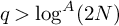 . Then one has

where
$B=\big ( \frac {2}{p}-1\big ) \sigma A-1+\frac {1}{p}$
 .
.
Proof. The hypotheses concerning
$\theta $
 ensure that the methods of Vinogradov and Hua (see [Reference Hua13, Reference Vinogradov25]) show that there is a positive number
$\sigma =\sigma (k)$
ensure that the methods of Vinogradov and Hua (see [Reference Hua13, Reference Vinogradov25]) show that there is a positive number
$\sigma =\sigma (k)$
 having the property that

uniformly in
$\beta $
 . Thus, with
$f(n)=\Lambda (n)e(n^k\theta )$
. Thus, with
$f(n)=\Lambda (n)e(n^k\theta )$
 , one has
$\|H_f\|_\infty \ll \log ^{-\sigma A}(2N)$
, one has
$\|H_f\|_\infty \ll \log ^{-\sigma A}(2N)$
 and
and

Hence, we deduce from Theorem 7.1 that

The desired conclusion now follows.
By way of illustrating the potential for applications, we note that on taking A sufficiently large, the conclusion of Corollary 7.3 would offer minor arc estimates of use in investigating k-th powers of prime numbers
$\pi $
 in which
$\pi +2$
in which
$\pi +2$
 belongs to a subconvex
$L^p$
belongs to a subconvex
$L^p$
 -set such as a Beatty sequence, or the set of square-free numbers, or indeed the square-free numbers belonging to a Beatty sequence.
Estimates for exponential sums with cusp form coefficients exhibit non-trivial cancellation when restricted to subconvex
$L^p$
 -sets.
Corollary 7.4. Suppose that

is a cusp form of weight
$k>0$
 for a discrete group
$\Gamma $
for a discrete group
$\Gamma $
 for which
$\infty $
for which
$\infty $
 is a cusp of width
$1$
is a cusp of width
$1$
 . Then, whenever
$\mathscr A$
. Then, whenever
$\mathscr A$
 is a strongly subconvex
$L^p$
is a strongly subconvex
$L^p$
 -set for some real number p with
$1\leqslant p<2$
-set for some real number p with
$1\leqslant p<2$
 , one has

Proof. We apply Theorem 7.1 with
$f(n)=a(n)$
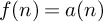 . Here, as a consequence of Iwaniec [Reference Iwaniec15, Theorem 5.3], one has

whilst [Reference Iwaniec15, Theorem 5.1] provides the bound

Consequently, we see from Theorem 7.1 that

This completes the proof of the corollary.
By way of comparison, the bound [Reference Iwaniec15, Theorem 5.3] shows that

whilst by applying the trivial estimate
$|a(n)|\ll n^{k/2}$
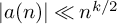 , one finds that

Thus, Corollary 7.4 saves roughly a factor
$N^{1/p}$
 over the trivial estimate, and as p approaches
$1$
over the trivial estimate, and as p approaches
$1$
 the conclusion of Corollary 7.4 approaches the strength of the bound (7.1) applicable to unrestricted sums.
This circle of ideas also addresses character sums restricted to subconvex
$L^p$
 -sets. We provide an illustration of the possible conclusions in this direction.
Corollary 7.5. Let
$\chi $
 be a non-principal character modulo
$\pi $
be a non-principal character modulo
$\pi $
 , with
$\pi $
, with
$\pi $
 a prime number. Suppose that
$\mathscr A$
a prime number. Suppose that
$\mathscr A$
 is a strongly subconvex
$L^p$
is a strongly subconvex
$L^p$
 -set for some real number p with
$1\leqslant p<2$
-set for some real number p with
$1\leqslant p<2$
 . Then, whenever r is a positive integer exceeding
$1$
. Then, whenever r is a positive integer exceeding
$1$
 , one has

Proof. We apply Theorem 7.1 with
$f(n)=\chi (n)$
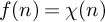 . Here, as a consequence of Chamizo [Reference Chamizo9, Theorem 1.1], one has

whilst
$\|f\|_{l^2(N)}\leqslant 1$
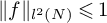 . Consequently, we find that the desired conclusion is immediate from Theorem 7.1.
Notice that the conclusion of Corollary 7.5 confirms that non-trivial cancellation occurs in the character sum

whenever
$N>\pi ^{\frac {r}{4r-4}}(\log \pi )^{\frac {1}{2}}$
 . Thus, whenever
$\varepsilon>0$
. Thus, whenever
$\varepsilon>0$
 , we may take r sufficiently large in terms of
$\varepsilon $
, we may take r sufficiently large in terms of
$\varepsilon $
 so as to ensure that non-trivial cancellation occurs provided only that
$N>\pi ^{1/4+\varepsilon }$
so as to ensure that non-trivial cancellation occurs provided only that
$N>\pi ^{1/4+\varepsilon }$
 .
.
A final example helps to underscore the flexibility of our methods.
Corollary 7.6. Let
$t(n)$
 denote the Fourier coefficient associated with a Maass form
$\psi $
denote the Fourier coefficient associated with a Maass form
$\psi $
 for the full modular group, corresponding to an eigenvalue
$\tfrac {1}{4}+r^2$
for the full modular group, corresponding to an eigenvalue
$\tfrac {1}{4}+r^2$
 of the hyperbolic Laplacian, so that

Suppose that
$\mathscr A$
 is a strongly subconvex
$L^p$
is a strongly subconvex
$L^p$
 -set for some real number p with
$1\leqslant p<2$
-set for some real number p with
$1\leqslant p<2$
 . Then, for large N, one has

Proof. We apply Theorem 7.1 with
$f(n)=t(n)$
 . In this setting, as a consequence of Epstein, Hafner and Sarnak [Reference Epstein, Hafner and Sarnak11, Theorem 3.1], one has

uniformly in
$\beta $
 , whilst [Reference Epstein, Hafner and Sarnak11, equation (2.2)] confirms that
$\|f\|_{l^2(N)}\ll 1$
, whilst [Reference Epstein, Hafner and Sarnak11, equation (2.2)] confirms that
$\|f\|_{l^2(N)}\ll 1$
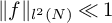 . Consequently, the desired conclusion is immediate from Theorem 7.1.
We should note that, although we have restricted ourselves in this section to problems involving strongly subconvex
$L^p$
 -sets, this is not an essential hypothesis. Were we to modify our hypotheses throughout to consider weakly subconvex
$L^p$
-sets, this is not an essential hypothesis. Were we to modify our hypotheses throughout to consider weakly subconvex
$L^p$
 -sets, then a self-evident adaptation of our methods would yield the same upper bounds in every conclusion, save that an additional factor of
$N^\varepsilon $
-sets, then a self-evident adaptation of our methods would yield the same upper bounds in every conclusion, save that an additional factor of
$N^\varepsilon $
 should be inserted throughout. We note further that the examples described above provide just some of many possible applications of the ideas within the orbit of this memoir. Moreover, more sophisticated strategies are suggested when information concerning
$4$
should be inserted throughout. We note further that the examples described above provide just some of many possible applications of the ideas within the orbit of this memoir. Moreover, more sophisticated strategies are suggested when information concerning
$4$
 -th and higher moments of
$H_f(\alpha ;N)$
-th and higher moments of
$H_f(\alpha ;N)$
 is available, as is often the case. The basic message to be borne away from this discussion is that subconvex
$L^p$
is available, as is often the case. The basic message to be borne away from this discussion is that subconvex
$L^p$
 -sets lend themselves well to problems involving averages of arithmetic functions.
8 Subconvex
$\boldsymbol{L^p}$
-sets modulo q

In certain applications of subconvex
$L^p$
 -sets in number theory, it may be convenient to work with discrete rather than continuous moments. As a model example of such a scenario, consider a natural number q and the discrete moment

Our principal result in this section is the analogue of the mean value estimate (1.3) for strongly subconvex
$L^p$
 -sets
$\mathscr A$
-sets
$\mathscr A$
 provided by Theorem 1.6.
The proof of Theorem 1.6.
We adjust the notation (3.2) by writing

Thus, when
$1<p<2$
 , one has

Equipped with this relation, we seek to convert the discrete mean value
$S_p(N;\mathscr A;q)$
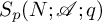 into a continuous analogue by applying the Sobolev-Gallagher inequality (see [Reference Montgomery21, Lemma 1.1]). Thus, whenever
$a\in \mathbb Z$
into a continuous analogue by applying the Sobolev-Gallagher inequality (see [Reference Montgomery21, Lemma 1.1]). Thus, whenever
$a\in \mathbb Z$
 and
$q\in \mathbb N$
and
$q\in \mathbb N$
 , we have

When
$f_N(\beta +a/q)\ne 0$
 , it follows from (8.3) that

whence

Since
$p>1$
 , we therefore deduce from (8.1) that

We must now bound mean values involving
$f^{\prime }_N(\alpha )$
 in terms of mean values involving
$f_N(\alpha )$
in terms of mean values involving
$f_N(\alpha )$
 . For this purpose, we draw inspiration from the argument following [Reference Wooley27, equation (3.2)]. We observe that

Recall the definition (8.1). Then, on writing
$\mathscr A(N)=\{ a_1,a_2,\ldots ,a_M\}$
 , with

we see that the sum on the right hand side here may be rewritten via partial summation in the form

We therefore see that for all real numbers
$\alpha $
 , one has

An application of the Carleson-Hunt theorem (see [Reference Hunt14, Theorem 1]) in the form given by Bombieri [Reference Bombieri5, page 12] shows that

We therefore deduce that whenever
$\mathscr A$
 is a strongly subconvex
$L^p$
is a strongly subconvex
$L^p$
 -set, then one has

We now substitute the estimate (8.5) into (8.4) following an application of Hölder’s inequality. Thus, on applying once again the hypothesis that
$\mathscr A$
 be a strongly subconvex
$L^p$
be a strongly subconvex
$L^p$
 -set, we find that

This delivers the conclusion of the theorem.
In order to demonstrate the utility of this mean value estimate, we note an application to character sums that in many circumstances provides an alternative to the estimate given in Corollary 7.5.
Corollary 8.1. Let q be a large natural number, and suppose that
$\chi $
 is a primitive character modulo q. Let p be a real number with
$1<p<2$
is a primitive character modulo q. Let p be a real number with
$1<p<2$
 , and suppose that
$\mathscr A$
, and suppose that
$\mathscr A$
 is a strongly subconvex
$L^p$
is a strongly subconvex
$L^p$
 -set. Then, one has

Proof. We recall the notation (8.2), and in addition define

Then, by orthogonality, one sees that

An application of Hölder’s inequality reveals, therefore, that

Since we assume
$\chi $
 to be primitive, it follows from [Reference Montgomery and Vaughan22, Theorem 9.7] that
$|T(a)|\leqslant \sqrt {q}$
to be primitive, it follows from [Reference Montgomery and Vaughan22, Theorem 9.7] that
$|T(a)|\leqslant \sqrt {q}$
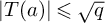 . Thus, by orthogonality, we see that whenever
$1<p<2$
. Thus, by orthogonality, we see that whenever
$1<p<2$
 , one has

We therefore deduce from Theorem 1.6 and (8.6) that

This yields the conclusion of the corollary.
Notice that as
$p\rightarrow 1$
 , the estimate provided by Corollary 8.1 has strength approaching the classical estimate of Pólya-Vinogradov (see [Reference Montgomery and Vaughan22, Theorem 9.18], for example). Meanwhile, our estimate remains non-trivial for all values of p smaller than
$2$
, the estimate provided by Corollary 8.1 has strength approaching the classical estimate of Pólya-Vinogradov (see [Reference Montgomery and Vaughan22, Theorem 9.18], for example). Meanwhile, our estimate remains non-trivial for all values of p smaller than
$2$
 .
.
Competing interests
The author has no competing interests.
Data availability statement
There is no data associated with this paper.


 Open access

