


1. Introduction
The deployment of artificial intelligence (AI) can significantly increase the productivity of industrial companies by automating complex tasks (Reference Czarnitzki, Fernández and RammerCzarnitzki et al., 2023). Thus, in product development, tasks based on complex physical principles and whose solution is partly built on trial and error, such as design adaptations, can be automated using Reinforcement Learning (RL) (Reference Ng, Chen, Lee, Jiao and YangNg et al., 2021; Reference Panzer and BenderPanzer & Bender, 2022). However, these design adaptations can have various objectives, which are defined in the associated Design for X (DfX). Examples include Design for Manufacture and Design for Strength. So, the information relevant to decision-making is defined by the specific DfX goal. (Reference Bauer and MeerkammBauer & Meerkamm 2007; Reference Holt and BarnesHolt & Barnes, 2010) Integrating this specific information into the RL state can improve the efficiency of design adaptations by reducing the number of simulations required while maintaining or improving design performance. To quantify the impact of structured adaptation-specific information in the RL algorithm on the efficiency of the design adaptation, ablation studies are conducted. In these ablation studies, additional information is systematically added to an initially sparse state (initial value) in order to analyse the influence of the individual state enrichments on the result separately. To this end, task-relevant additional information is first collected and classified, and then converted into states with varying degrees of enrichment. These states are thereafter tested for their associated sample efficiency and policy quality which characterise the efficiency of design adaptations. Conclusions about the benefit of the state enrichments are drawn from direct comparisons. By holding the RL algorithm, reward, and action space constant, this approach isolates the influence of the individual additional information on the learning dynamics.
2. State of the art
RL is a subfield of machine learning (ML). Its functionality can be seen in Figure 1. An agent maps each state of an environment to an action and receives a reward as feedback, which assesses the achievement of specified goals in the new state. A state is the agent’s observation of the environment. Following the prior action, a new action is selected and executed for the new state. The aim is to determine a policy that maximises the long-term reward. (Reference Sutton and BartoSutton & Barto, 2014) This can be achieved using deep Q-learning, a technique which optimises sequential decision-making processes, such as design adaptations. This is accomplished by approximating the expected discounted cumulative future reward (Q-values) using Deep Q-Networks (DQNs). (Reference Mnih, Kavukcuoglu, Silver, Rusu, Veness, Bellemare, Graves, Riedmiller, Fidjeland, Ostrovski, Petersen, Beattie, Sadik, Antonoglou, King, Kumaran, Wierstra, Legg and HassabisMnih et al., 2015; Reference Watkins and DayanWatkins & Dayan, 1992)
In deep Q-learning, the Q-values are calculated based on the state (Reference Mnih, Kavukcuoglu, Silver, Rusu, Veness, Bellemare, Graves, Riedmiller, Fidjeland, Ostrovski, Petersen, Beattie, Sadik, Antonoglou, King, Kumaran, Wierstra, Legg and HassabisMnih et al., 2015). However, setting up the state requires considering the Markov property. This means that calculating the next state and expected reward depends only on the current state and action. (Reference Sutton and BartoSutton & Barto, 2014)
Schematic functionality of RL in accordance to Reference Sutton and BartoSutton and Barto (2014)

In product development, RL states are modelled differently depending on the application. In Reference Dworschak, Dietze, Wittmann, Schleich and WartzackDworschak et al. (2022), a state vector is used to optimise bicycle components. This vector represents parameters that can be directly adapted by the RL, such as sheet thicknesses or hole diameters. A similar approach is used in Reference Brown, Garland, Fadel and LiBrown et al. (2022), where the elements of a 2D discretised topology to be adapted are represented directly within a state grid. As the locations of the supports and forces are marked on the grid alongside the topology, this state representation provides a more precise description of the physical mechanisms. However, the explicit encoding of causal and physics-based mechanisms in the state and the analysis of their influence on the result are rarely applied in the field of RL for structural design adaptations. Nevertheless, the learning time of RL can be improved by using causal and physically meaningful state representations, for example by integrating Lagrange multipliers into the state in order to solve RL problems with multiple conditions (Reference Banerjee, Nguyen, Fookes and RaissiBanerjee et al., 2025; Reference Calvo-Fullana, Paternain, Chamon and RibeiroCalvo-Fullana et al., 2023). However, the state modelling requires a trade-off to be found, because states with insufficient information lead to suboptimal policies, while states with redundant information result in increased complexity and a greater number of samples being required for the training of the network (Reference Huang, Lu, Leqi, Hernández-Lobato, Glymour, Schölkopf and ZhangB. Huang et al., 2022).
Furthermore, these current approaches for structural design adaptations operate on vector- or grid-based states that have a fixed size. In contrast, Reference Hayashi and OhsakiHayashi & Ohsaki (2020) and Reference Hayashi and OhsakiHayashi & Ohsaki (2021) optimise trusses by representing the states as graphs. Here, the joints are represented as nodes and the beams as edges, whereby adjacent joints are directly connected. Graph neural networks (GNNs) are used to process this state. Compared to grid- and vector-based states and their processing with multi-layer perceptrons (MLPs), this setup offers advantages in terms of the size and structure of the inputs that can be processed, as these are not limited to fixed grid sizes. In addition, causal and physical relations can be explicitly encoded in graphs.
In general, GNNs have different characteristics than MLPs, which have to be considered when adapting designs using GNN-based RL. GNNs directly utilise the graph structure and learn from the interactions between graph neighbours through message passing between neighbouring nodes, whereas classical MLPs treat all inputs equally and cannot explicitly model relationships (Reference Gilmer, Schoenholz, Riley, Vinyals and DahlGilmer et al., 2017; Reference Wu, Cui, Pei and ZhaoWu et al., 2022). Working on the basis of graph structure leads to permutation invariance because graphs have no explicit node order. This also enables GNNs to be used for graphs of various sizes originating from the same domain. (Reference Zhou, Cui, Hu, Zhang, Yang, Liu, Wang, Li and SunZhou et al., 2020) By contrast, MLPs cannot be used directly for different state sizes. For new state sizes, MLPs would have to be adapted to the new input size and retrained from scratch. Furthermore, with sufficient connectivity, the generalisation capability to new use cases is higher for GNNs than for MLPs due to its signal learning (Reference Huang, Cao, Wang, Cao and SuzukiW. Huang et al., 2025). However, it should be noted that excessive edge density can lead to oversmoothing during the processing of the graph in the GNN, which impairs the network’s learning ability. In graphs with too many edges, the nodes lose their distinctiveness during message passing and become increasingly homogeneous. (Reference Wu, Cui, Pei and ZhaoWu et al., 2022) Furthermore, low sample efficiency is a potential shortcoming of graph-based approaches (Reference Awasthi, Das and GollapudiAwasthi et al., 2022).
3. Research gap
Although some research has already used RL to automate design adaptations, whose states are partly enriched with additional information, the influence of various types of additional information on the efficiency of design adaptations has not yet been systematically investigated. This means, it is unclear what additional benefit each type of information provides in terms of the efficiency of RL-based design adaptations.
Furthermore, the states of the structural mechanical optimisation are usually represented in a vector- or grid-based manner. So, in parametric design adaptation, each element that can be adapted is represented by an input neuron (Reference Dworschak, Dietze, Wittmann, Schleich and WartzackDworschak et al., 2022). However, these approaches can only be applied to components with the same structural design and the same number of parameters to be adapted. For example, when optimising the ply thicknesses of fibre-reinforced composites with eight plies, the network can only be used for composites with eight plies without changing the network architecture and retraining, which severely limits its practical usability in product development. The utilization of GNN-based RL helps to overcome these limitations, since they can process different numbers of components represented by nodes. Another advantage of these GNN-based approaches is that additional information can be represented not only in the graph’s features, but also via edges indicating structural relationships between components (e.g., to indicate symmetry or load paths). This can enhance the causal and physical description of the state.
However, it remains to be investigated how enriching the GNN-based state with structural information improves the efficiency of RL-automated design adaptations without facing issues such as oversmoothing. This raises the following research question: How do different levels of additional task-relevant structured information embedded in the GNN-based RL-state influence the efficiency of automated design adaptations?
To answer the research question and assess the efficiency of automated design adaptations, ablation studies are conducted. Herein, the effect of additional information on the sample efficiency and policy quality, which characterise the efficiency of design adaptations, is analysed. The chosen domain example is the optimisation of the thicknesses and fibre orientations of the plies of a fibre-reinforced composite component, which has strong mutual relationships between the individual plies.
4. Methodical approach
The methodical approach of analysing the states enriched with different levels of task-relevant information in terms of efficiency of automated design adaptations is shown in Figure 2. First, it is necessary to determine which engineering information can be used in the state. This information is identified and classified into categories in Section 4.1. In Section 4.2, these categories are converted into graphs with varying degrees of information to form different state variants. Subsequently, in Section 4.3, GNN-based RL algorithms are trained with these various variants as respective states. During training, ablation studies are carried out at regular intervals to evaluate the effect of individual state changes on the sample efficiency and policy quality.
Overview of the methodical approach

4.1. Definition of possible information enrichment within the state
In addition to the parameters that can be adapted directly by the agent, the state may contain other influencing parameters for a design adaptation. To determine these influencing parameters, the goal of design adaptation according to DfX must first be clarified. From this goal, the influencing parameters can be derived. These parameters are physically based and used by engineers in design adaptation tasks. In order to test the amount of additional information required to increase the efficiency of design adaptations, these influencing parameters must first be classified into categories. For this purpose, a distinction is made between task-relevant features (such as the location of forces) and the resulting properties derived from them (such as stress values).
However, additional information can be expressed not only by parameters such as features and properties, but also by causal, physically based relations between design elements, for example, regarding adjacencies, force paths and symmetries. Therefore, various types of relationship between the design elements are distinguished in order to assess their impact on sample efficiency and policy quality.
4.2. Transfer to various information-enriched graphs
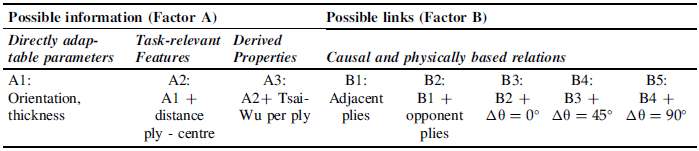
In physical systems such as mechanically stressed designs, the components and parameters are interrelated. To model this in the proposed graph-based approach, components are represented by nodes and their relations by edges. This allows information such as directly adaptable parameters, task-relevant features and derived properties to be described in the node features of the individual components, while causal, physically based relations can be represented by edges. To avoid unnecessary effort and oversmoothing, the effects of different amounts of information described in the respective states are tested within ablation studies. In order to isolate the effects of various changes in the state representations, two factors are defined:
Factor A — Node-feature content:
-
• A1: node features contain only the directly adaptable parameters
-
• A2: A1 plus additional task-relevant features (e.g., location/magnitude of forces)
-
• A3: A2 plus additional task-relevant properties derived from respective features (e.g., stresses)
Factor B — Edge set/edge density:
-
• B1: adjacency edges only (i.e., edges between neighbouring components; minimum number of edges in a graph)
-
• B2: B1 plus a set of semantically meaningful, task-relevant edges (e.g., symmetry edges)
-
• B3-Bx: various edge-sets which progressively densify with further task-relevant edges beyond B2 up to a fully connected graph (fully connected = maximal number of edges in a graph)
This results in the following sets of states, in which only one information class changes between variants, enabling the direct identification of the effects of the changes:
-
• A1 x B1: sparse state with the directly adaptable parameters and basic adjacent edges to represent the baseline
-
• A1 x B2: previous combination plus task-relevant edges to allow individual assessment of the influence of extra task-relevant edges on sample efficiency and policy quality
-
• A2 x B2: extension of the graph features from the previous combination with additional task-relevant features to assess their influence on the result
-
• A2 x B3-Bx: previous combination plus additional semantically relevant edges to find the trade-off between information density and edge density
-
• A3 x B2 and A3 x B3-Bx: extension of the node features from the two previous combinations with additional properties derived from the task-relevant features in order to assess the effect of these properties
Across all conditions, the other constraints such as the RL algorithm, the reward function, and the action space are constant to enable causal attribution to the state design.
4.3. Assessing sample efficiency and policy quality through ablation studies
A GNN is used to process the different state sets and calculate action-specific Q-values. Herein, node embeddings that contain both local and global information are built through edge-conditioned convolutions and message passing. These node embeddings are then processed by an MLP to calculate the Q-values. Only one MLP is required for all node embeddings, as one of three possible actions can be performed for each component: increase, decrease or keep the same. To reduce the action space, however, only one component can be adapted per step.
To validate the efficiency of the automated design adaptation process, the associated RL is evaluated every 100 steps during training. This is achieved by using known and randomly generated component configurations with different seeds, in order to robustly assess sample efficiency and policy quality. This frequency strikes a balance between monitoring the quality of the agent’s policy and avoiding prolonging training unnecessarily. This is because, during these checks, the network processes new test cases whose stress properties must be simulated. During these checks, the policy is frozen, meaning it cannot learn from the test cases through backpropagation. This makes the results of the different variants comparable. Additionally, to prevent random actions, the agent acts continuously without exploring. This also promotes comparability, as no good random actions can be taken by chance during the checks.
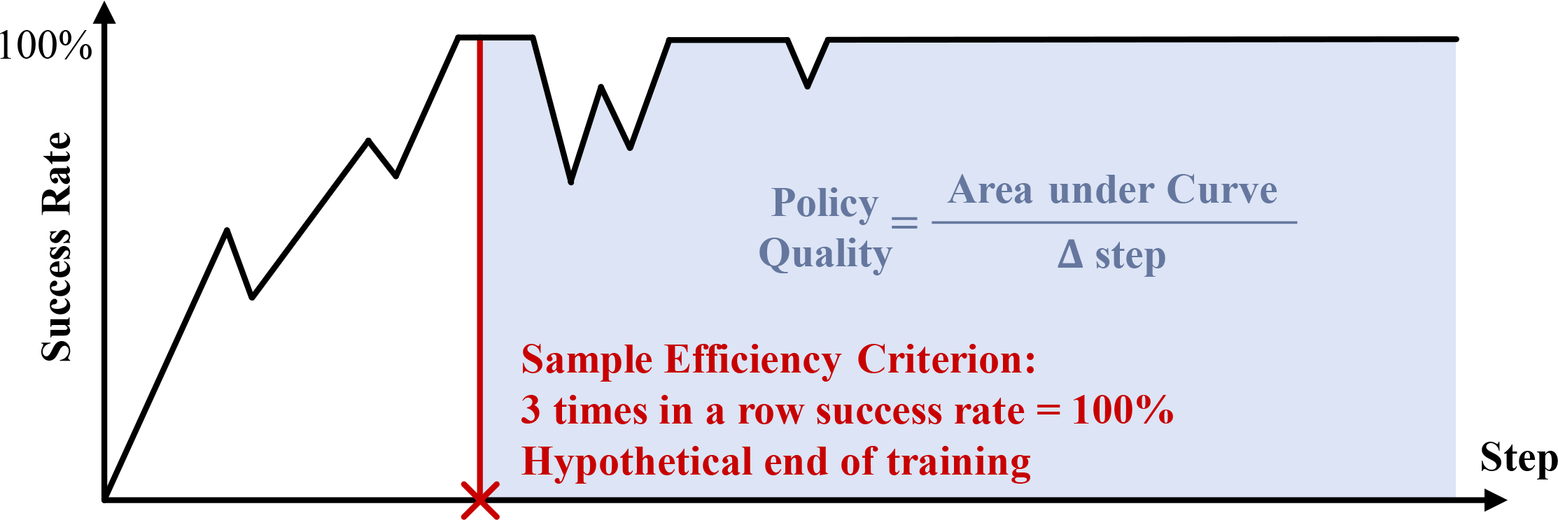
During these evaluation checks, the percentage of runs that meet the adaptation goals of the respective test cases is logged (success rate). Sample efficiency is measured as the number of unique simulation calls (unseen samples) required to first reach three consecutive episodes in which all adaptation goals are achieved. The criterion of three consecutive episodes with a success rate of 100% prevents a random success from distorting the result. So, this criterion can be used to assess when the RL understands how to solve the task. Consequently, it could be used to determine the end of the training. To assess the policy quality, the focus is on the period after this sample efficiency criterion has been reached, as few conclusions about the long-term policy can be drawn from the previous period, when correlations are being learned. So, to analyse the policy quality, the area under the success rate (Area under Curve; AUC) is calculated after reaching the sample efficiency criterion and related to the change in the step number. This calculates the average success rate of the policy at the evaluation checks. Figure 3 shows the schematic determination of the sample efficiency and the policy quality.
Schematic representation of the measurands to assess the sample efficiency and policy quality

5. Study - simultaneous adaptation of the ply thickness and fibre orientation in a fibre-reinforced composite design
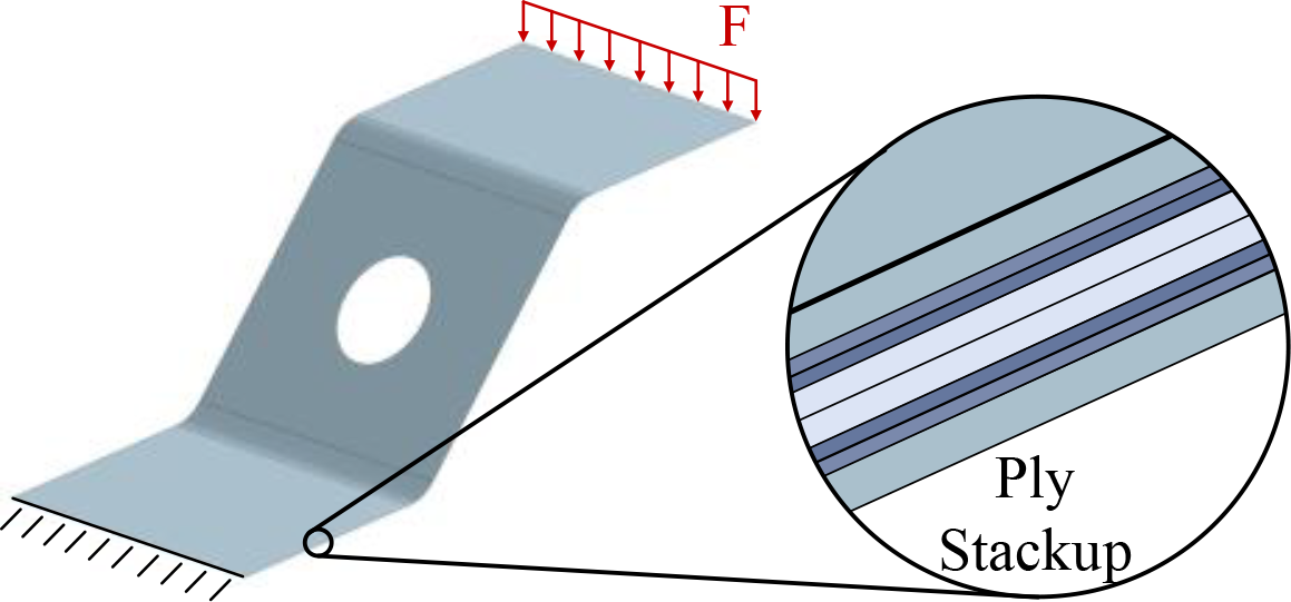
This methodical approach is applied to the stress-based design adaptation of fibre-reinforced composites. The composite structure is therefore represented by a graph, with the plies represented by nodes. To avoid distortion, the ply stack-up is made symmetric, meaning that the fibre orientation and thickness of opposite plies are equal. The fibre orientation and ply thickness influence the stresses in the design. (Reference CardarelliCardarelli, 2008) Thus, these parameters are adapted within the RL-based design adaptation to ensure compliance with the permitted stress.
In the case under consideration, represented in Figure 4, the agent can simultaneously adapt the thicknesses and fibre orientations of a composite built of eight plies. The ply thicknesses can be adapted in 0,1 mm increments within the range [0,2 mm, 0,4 mm], and the fibre orientations in 45° increments within the range [0°, 135°]. This results in 20.736 possible combinations.
Representation of the load case in the application example

The strength of anisotropic materials such as the considered fibre-reinforced composites can be evaluated using the Tsai-Wu failure criteria (Reference Tsai and WuTsai & Wu, 1972). To this end, the design adaptation is assessed using the Tsai-Wu value per ply. The adapted components are simulated using the Python interface of Ansys 2024 R2 to determine the Tsai-Wu distribution for each ply. To avoid reducing the Tsai-Wu value simply by increasing ply thickness, an additional weight-related condition is introduced.
5.1. Definition of the possible information contained within the different states
Firstly, the information that could be contained within the state are analysed. According to Section 4.1, the directly adaptable parameters, additional task-relevant features and properties derived from them, as well as causal, physically based relations between the plies, are investigated.
The directly adaptable parameters are represented by the fibre orientation and thickness of each ply of the laminate. Regarding additional task-relevant features, the distance of a ply to the middle of the laminate can be used to calculate the bending stiffness (Reference JonesJones, 1999). This distance is thus task-relevant and can therefore be included in the state, making this information available to the agent. In addition, properties derived from the features can also be used to enrich the state. These are directly related to the adaptation goal. To provide the agent with this kind of information, the maximal Tsai-Wu value per ply can be included in the respective nodes. This enables the agent to observe the intermediate effects of its actions and learn which node to adapt to achieve the adaptation goal.
In terms of causal, physically based relations, three relation types can be encoded: adjacency between neighbouring plies (bonded interfaces), symmetry between opposite plies in symmetric laminates, and orientation-dependent coupling between ply pairs, which represents the mechanical correlations through fibre orientation difference ${\rm{\Delta \theta}}$
(Reference Memarzadeh, Onyibo, Asmael and SafaeiMemarzadeh et al., 2024). To define discrete information levels,
${\rm{\Delta \theta}}$
(Reference Memarzadeh, Onyibo, Asmael and SafaeiMemarzadeh et al., 2024). To define discrete information levels,
 $${\rm{\Delta \theta }}$$
is discretized into
$${\rm{\Delta \theta }}$$
is discretized into
 $$\left\{ {0^\circ ,45^\circ ,90^\circ } \right\}\;$$
with
$$\left\{ {0^\circ ,45^\circ ,90^\circ } \right\}\;$$
with
 $${\rm{\Delta \theta }} = 90^\circ $$
as the maximum fibre orientation difference. According to Section 4.2, Table 1 shows the possible information, which can be represented within the state.
$${\rm{\Delta \theta }} = 90^\circ $$
as the maximum fibre orientation difference. According to Section 4.2, Table 1 shows the possible information, which can be represented within the state.
Contribution of the possible information in the state

5.2. Building graphs with several levels of information
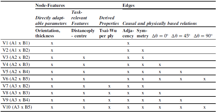
Ten state variants are tested (see Table 2). This set is derived from the test plan outlined in Section 4.2 and the definition of possible information within the state, as detailed in Section 5.1.
Set of various state variants

5.3. Investigating sample efficiency and policy quality through evaluation checks
Evaluation checks are conducted every 100 steps. These evaluation checks consist of test cases with the following initial thicknesses and fibre orientations, which the RL must adapt in order to achieve the strength-based goal:
-
1. Thickness of 0,2 mm and fibre orientation of 0° for all plies, respectively: tested three times with three different seeds
-
2. Thickness of 0,4 mm and fibre orientation of 90° for all plies, respectively: tested three times with three different seeds
-
3. Random thicknesses and fibre orientations within the borders for all plies, respectively: three different variants tested with different seeds
The first two variants, with initial ply thicknesses of 0,2 mm or 0,4 mm and initial fibre orientations of 0° or 90°, are chosen to cover the border area. Testing these variants with different seeds, as well as variants of random thicknesses and fibre orientations with different seeds, ensures robust results. To analyse the efficiency of the design adaptation, the step is investigated at which all checks for the nine combinations have been passed three times in a row with a 100% success rate. Then, the agent could solve a total of 27 different combinations (9 combinations x 3 checks) in a row, 9 of which were chosen completely at random. Afterwards, the relative success rate is calculated to assess the quality of the respective policy.
5.4. Results of the evaluation checks
The results of the evaluation checks within the training sessions of V1 - V10, each consisting of 500 episodes with 20 steps (10.000 steps in total), are depicted in Figure 5.
Resulting curves (blue) of the evaluation checks with indication of the sample efficiency criterion (red dotted)

In addition, Table 2 lists the step and the corresponding sample size when all evaluation checks were passed 100% three times in a row (sample efficiency criterion), as well as the average relative success rate after that point to indicate the long-time quality of the policy.
Representation of the step number until reaching the sample efficiency criterion, the corresponding sample size and the average success rate

5.5. Analysis of the results of the ablation studies
The information classes of the graphs are analysed. This involves comparing the results of the sparse graph V1, the graph with additional causal and physically based edges V2, the graphs with additional task-relevant features (V3–V6) and the graphs with extra properties derived from them (V7–V10) to investigate the type of information that helps the agent choose the right actions. Furthermore, the influence of edge density on sample efficiency and policy quality is analysed.
Adding causal edges to the baseline graph: V1, the sparse baseline graph, requires 5.200 steps and 2.369 samples to achieve the adaptation goal of all test cases within the evaluation checks three times in a row. The average success rate after this point is 78,5%. This means that after step 5.200, in 78,5% of test cases during the evaluation checks, the adaptation goal is achieved. Adding task-relevant edges (V2) improves the number of steps (4.200; -19,2%) and the sample size (2.073; -12,5%) until the sample efficiency criterion is reached, as well as the average success rate afterwards (and thus the quality of the policy). V2 has an average success rate of 93.7%, which is 19,4% higher than V1’s. This can be attributed to the enhanced flow of information through the additional edges.
Adding task-relevant features: The final average success rate and thus the quality of the policy can be increased by providing extra task-relevant features. This can be seen from the final success rate of V3 (97,9%; +4,5%). This is because the graph of V3 more accurately describe the physical system by adding physically based decision-relevant parameters.
Adding causal and physically based edges (until the graph is fully connected): The edge density of the combinations V3 - V6 is now being analysed to investigate the impact of edge number on the results. The highest success rates are shown in graphs V3 and V5. V3’s high success rate is due to the fact that its edges are constant and do not depend on the state. However, the edges of V4 and V5 depend on differences in fibre orientation and are thus dynamic. Graphs with dynamic edges can increase the complexity and decrease the efficiency of GNNs (Reference Zheng, Yi and WeiZheng et al., 2025). This increase in complexity stems from an increase in the size of the state space. While V5 can overcome this difficulty thanks to its greater amount of information and more precise description of the physical system, the efficiency of V4 is comparatively low due to its limited information input and dynamic edges. Like V3, V6 has constant edges, but in contrast to V3, V6 is a fully connected graph. However, due to the high edge density of V6 and the subsequent oversmoothing (Reference Wu, Cui, Pei and ZhaoWu et al., 2022), its quality of the policy is lower.
The main observations also hold for the Tsai–Wu–enriched variants (V7–V10). In graphs with constant edges (V7 and V10), the quality of the policy is lower for fully connected graphs. In contrast, in graphs with dynamic edges (V8 and V9), adding edges and hence more information improves the efficiency of design adaptations.
Adding properties derived from the task-relevant features: Enriching the state with properties such as Tsai-Wu values decreases the final average success rate of the policies. This is made evident by comparing the final average success rate of the respective graphs, once with and once without additional properties derived from task-relevant features (V7: 94,0%, −4,0% compared to V3; V8: −; V9: 89,4%, −9,2% compared to V5; V10: 89,8%, -6,0% compared to V6). This is due to the fact that adaptations regarding ply thickness and fibre orientation can cause significant changes in the Tsai-Wu values of the plies. This is exacerbated by the fact that the state does not always contain the Tsai-Wu value of the same FE-element, but rather the maximum Tsai-Wu value across all FE-elements of a ply. Consequently, the FE-elements with the highest Tsai-Wu values change frequently. This amplifies the discontinuities, which are difficult for the agent to learn. On the other hand, the decrease in policy quality is due to the high correlation between the Tsai-Wu values in the state and the reward. Consequently, the agent quickly learns rigid, fragile approximations, resulting in steeper learning curves at the beginning of training. However, this can also cause issues when patterns change slightly or inaccuracies occur, resulting in a loss of policy quality. This faster learning process at the beginning of training is evident in the present results because if all adaptation goals are achieved three times in a row, both the associated step and sample size are generally lower than in the respective graphs V3-V6. However, this less robust policy, which includes a number of outliers, results in V8 not even reaching the sample efficiency criterion in the 10.000 training steps. This suggests that these graphs, which have additional properties derived from task-relevant features (regarding stress/RL-reward), reach the point faster at which they can automatically adapt these designs. However, the associated policy is less robust afterwards than for graphs with additional task-relevant features but without these extra properties.
6. Discussion
Ablation studies were conducted to investigate the influence of state enrichment with additional information on the efficiency of design adaptations, with direct comparisons of various graph variants. State variants that differ in only one aspect, such as the addition of extra stress properties, were investigated to identify the cause of different results. The factorial ablation design makes it possible to evaluate the contribution of node features (factor A) and edge sets (factor B) to the result separately.
In order to control random influences and thus assign the changes directly to the different state representations, different seeds are used. However, to ensure comparability between the individual state variants, identical seed tuples are used for all state variants (seed-matched comparison). The comparability between different state representations is also ensured by applying identical framework conditions for all state variants (same network, reward design, etc.). To obtain robust, reliable results, nine evaluation checks were performed every 100 steps, which is a good balance between coverage and effort, as these tests covered both edge cases and random combinations across different seeds.
The results suggest that enhancing sample efficiency while maintaining a high policy quality by enriching the state with additional information is advantageous when providing task-relevant features alongside the directly adaptable parameters. However, resulting properties such as stress-based Tsai-Wu values with a direct reference to the reward function can be included in the state if rapid automation results are required and lower policy quality is sufficient. Nevertheless, this promotes reward shortcuts and hampers the learning of real structural relations. Regarding edge density, fully connected graphs and graphs with dynamic edges and low information impact can decrease the policy’s quality.
With regard to the measurands and the results of the evaluation checks, the sample efficiency criterion is particularly vulnerable to interference as it provides a snapshot of a stochastic application. To mitigate this problem and reduce the influence of randomness, this measurand could have been selected with a certain degree of tolerance, for example by setting the average success rate in three consecutive evaluation checks to at least 95%. Nevertheless, the same general key findings would have emerged even with such definitions of the sample efficiency criterion.
In addition to the ability to directly assign edges and thus leverage relations to learn from structural patterns, graph-based machine learning applications offer advantages compared to vector- and grid-based networks in terms of transferability to other test cases with different sizes of the mechanical design (Reference Ruiz, Chamon and RibeiroRuiz et al., 2023). To avoid exceeding the scope of the work, only one fibre-reinforced composite with eight plies was tested. However, it is recommended to investigate the transferability of this approach to test cases with other ply sizes in future work.
7. Conclusion and outlook
This paper presents an analysis of how enriching the state of RL with additional task-relevant information affects the efficiency of automated design adaptations. The approach used graphs and GNNs to learn from additional information and structural patterns. The amount of information and its integration within the graph were tested. Therefore, various graph variants with different amounts of node features and edges were analysed in ablation studies. This approach was used in the context of strength-based design adaptations of a fibre-reinforced composite by simultaneously adapting thicknesses and orientations of the plies. However, the approach can also be applied to further design adaptations, which take place in the embodiment and final design stages, e.g., to ensure manufacturability or assemblability. To this end, additional parameters in the state, such as task-relevant features, and causal relations must be selected depending on the goals of the design adaptation.
The key finding is that enriching the state with additional information can make automated design adaptations more efficient. Even adding a few task-relevant relations between components in the state enhanced the efficiency in the tests. Further gains in efficiency were achieved by adding additional task-relevant features that are also considered by engineers when adapting designs. Adding properties derived from these features reduced the number of simulations until the RL learned the relevant relationships to adapt the design. However, the quality of the design adaptations decreased after this point compared to the variants with extra task-relevant features, but without additional properties derived from them.
Building on this work, the efficiency of automated design adaptations will be investigated by integrating not only the information used by product developers, but also their procedures into RL. This can be achieved by integrating design rules within the reward function of the RL.
Acknowledgement
Funded by the Deutsche Forschungsgemeinschaft (DFG, German Research Foundation) - 522180880.





 Open access

