

INTRODUCTION
Epidemic poliomyelitis was one of the important emergent viral diseases of the twentieth century [Reference Paul1, Reference Smallman-Raynor2]. While several lines of evidence point to the occurrence of poliomyelitis in pre-modern societies [Reference Hamburger3–Reference Dequeker, Fabry and Vanopdenbosch5], medical references to the disease prior to the nineteenth century are few in number and are consistent with the circulation of an endemic infection associated with sporadic cases of clinical disease [Reference Paul1]. Reports of small and highly localized outbreaks of ‘infantile paralysis' began to gain momentum in Europe from the 1880s. The world's first major epidemics occurred in Scandinavia in 1905 [Reference Wickman6–Reference Low9]. The same general sequence of poliomyelitis emergence (sporadic cases → small outbreaks → major epidemic events) was repeated during the late nineteenth and early twentieth centuries in other countries of Europe, North America and elsewhere [Reference Paul1, Reference Smallman-Raynor2, Reference May10]. By the 1950s, poliomyelitis had assumed the status of an epidemic disease of global proportions [Reference Paul1, Reference Smallman-Raynor2, Reference Nathanson and Kew11].
The emergence of epidemic poliomyelitis in twentieth-century England and Wales assumed a distinctive form, with a step-function transition to heightened epidemicity in the early post-war years (Fig. 1 a). Between the world wars, the monthly rate of poliomyelitis notifications in England and Wales rarely rose above 0·5 cases/100 000 population; 1926 and 1938 were the only years of epidemic note [Reference Bradford Hill12, Reference MacNalty and Cruickshank13]. The situation changed suddenly and markedly thereafter. Beginning with the first nationwide epidemic in 1947, England and Wales entered a decade-long phase of heightened poliomyelitis epidemicity [Reference Smallman-Raynor2]. This emergence profile differs from the experience of the USA where, in the wake of the epidemic of 1916, a relatively smooth and progressive transition to the major epidemic events of the post-war years was apparent (Fig. 1 b) [Reference Martin14, Reference Trevelyan, Smallman-Raynor and Cliff15]. On both sides of the Atlantic, the post-war period of heightened epidemicity was brought to a rapid close by the introduction and widespread administration of safe and effective poliovirus vaccines from the mid-1950s [Reference Paul1, Reference Smallman-Raynor2].
Monthly series of poliomyelitis notification rates per 100 000 population, 1913–1971. (a) England and Wales (source: General Register Office, London); (b) USA (source: Public Health Reports/Morbidity and Mortality Weekly Report).

The epidemic emergence of poliomyelitis in post-war England and Wales was accompanied by a pronounced change in the geography of the disease [Reference Martin14], with the replacement of small focal outbreaks (inter-war years) by large national epidemics (post-war years) signalling a fundamental shift in the spatial dynamics of disease propagation [Reference Bradford Hill12, Reference Hardy16]. An in-depth analysis of the geographical spread of the 1947 epidemic appears elsewhere [Reference Smallman-Raynor and Cliff17]. In the present article, we examine the shifting pattern of poliomyelitis activity with particular reference to the geographical rate of disease propagation in the 25-year sequence of poliomyelitis seasons, 1940–1964. Our examination draws on a robust method of spatial epidemiological analysis known as the swash–backwash model [Reference Cliff and Haggett18–Reference Cliff20]. This model is a spatial derivative of the generic SIR (susceptible ⇒ infected ⇒ recovered) mass action models commonly used to model the spread of infectious diseases in human and many animal populations [Reference Bailey21, Reference Anderson and May22]. Using the binary presence/absence of a disease rather than the actual number of notified cases in a set of districts, the swash–backwash model: (i) allows the identification of the leading and trailing edges of the spatial advance (‘swash’) and retreat (‘backwash’) of an infection wave; (ii) provides a means of measuring the phase transitions of geographical units from susceptible (S), through infective (I) and recovered (R) status as dimensionless integrals; and (iii) yields robust measures of the spatial velocity of epidemic waves from space–time series.
Our analysis demonstrates that the period of heightened poliomyelitis epidemicity in England and Wales, 1947–1957, was associated with a sudden and pronounced increase in the geographical rate of disease propagation. The change occurred in all types of geographical areas, affecting large, medium and small urban centres and rural districts alike.
METHODS
Data
Statutory case notifications of poliomyelitis in England and Wales have been collated by the General Register Office, London, since 1 September 1912 [23]. For the purposes of the present analysis, we drew on the weekly notifications of poliomyelitis (acute poliomyelitis and acute polioencephalitis) included in the Registrar General's Weekly Return of Births and Deaths … and Cases of Certain Specified Infectious Diseases (London: HMSO) for 1940–1964. For each of the 1305 registration weeks (ending on a Saturday) in the 25-year observation period, information on the number of notified cases of poliomyelitis in the 1479 standard local government districts (28 metropolitan boroughs, 83 county boroughs, 310 municipal boroughs, 576 urban districts and 482 rural districts; see Table 1) of England and Wales was abstracted from the Weekly Return to form a (1305 weeks × 1479 districts=) 1·93 million cell matrix of poliomyelitis notifications. This time–space matrix included records for a total of 69 928 cases of poliomyelitis.
Mean and range of mid-point population estimates for the 1479 standard local government districts of England and Wales at the beginning and end of the 25-year observation period, 1940–1964*

* Data from Registrar General's Statistical Review of England and Wales (London: HMSO).
† Population estimates in thousands.
The matrix cells for the constituent districts of each of the (then) 62 counties of England and Wales were grouped to form composite 1305-week time series of poliomyelitis notifications for each of three geographical divisions of a given county: (i) metropolitan and county boroughs, representing large urban areas; (ii) municipal boroughs and urban districts, representing medium and small urban areas; and (iii) rural districts (Table 1). Some categories of district were absent from some counties, so that the aggregation procedure resulted in a total of 152 county-specific time series: metropolitan and county boroughs, 31 counties; municipal boroughs and urban districts, 61 counties; and rural districts, 60 counties. The set of 152 time series (representing an exhaustive division of England and Wales) and the subsets of 31, 61 and 60 time series (representing different levels in the settlement system) form the basis of our analysis.
Defining the poliomyelitis season, 1940–1964
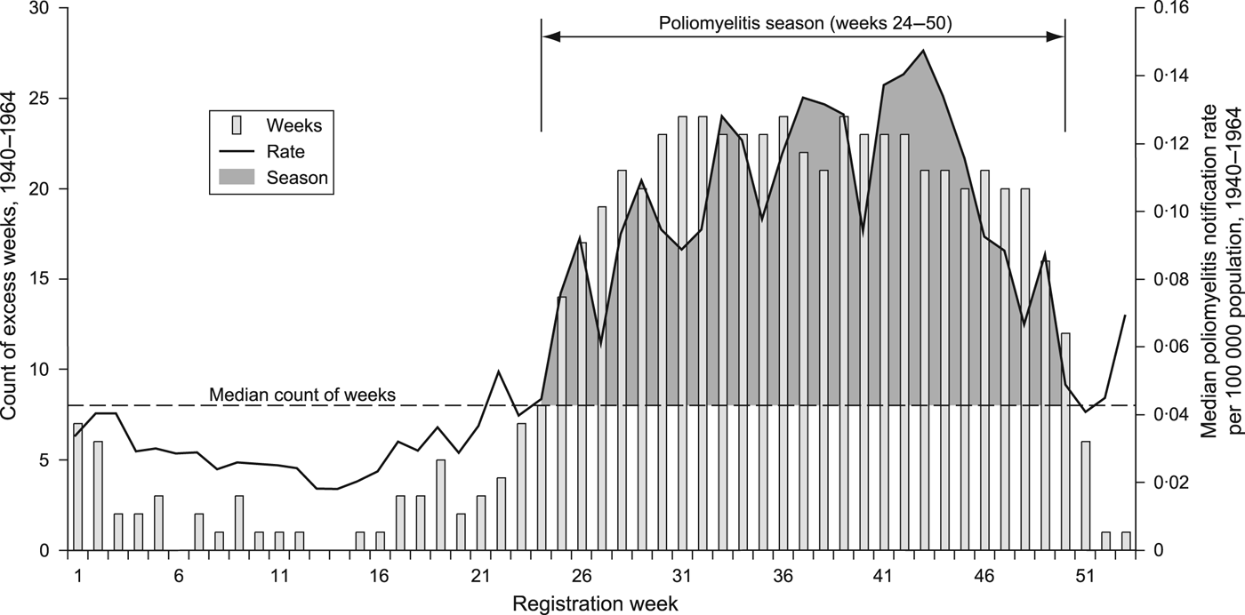
The seasonal proclivity of poliomyelitis is one of the outstanding epidemiological features of the disease [Reference Melnick, Evans and Kaslow24–Reference Fisman26]. During the inter- and early post-war years, the months of June–December formed the typical season of raised poliomyelitis activity in the temperate latitudes of the northern hemisphere [Reference Smallman-Raynor2]. To define formally the poliomyelitis season for England and Wales, 1940–1964, we adopted a robust method that apportioned equal weight to the temporal signal in each of the 25 observation years. The method, which is summarized in Figure 2, defines the poliomyelitis season as disease registration weeks 24–50 (mid-June to mid-December). Weekly time series of poliomyelitis notifications are plotted for successive poliomyelitis seasons in Figure 3; the aggregate count of notifications in each season, along with information on the predominant circulating virus type(s) isolated from patients with clinical disease, appears in Table 2.
The poliomyelitis season, England and Wales, 1940–1964. For a given year (1940, …, 1964), the count of poliomyelitis notifications in each registration week, w (1, …, 53) was assessed relative to the median weekly count of notifications for that year; weeks above the median were defined as ‘excess weeks'. The bar chart plots the number of years in which registration week w was categorized as an ‘excess week’ in the 25-year observation period. The median value of the set of bars (8) is demarcated by the broken horizontal line; registration weeks above this median are defined as constituting the poliomyelitis season (registration weeks 24–50). The heavy line trace is shown for reference and plots the median poliomyelitis notification rate per 100 000 population for registration week w in the period 1940–1964.
Time series of poliomyelitis notifications, England and Wales, 1940–1964. Graphs plot the weekly count of notifications for successive poliomyelitis seasons (registration weeks 24–50).

Application of the swash–backwash model to the 1940–1964 poliomyelitis seasons, England and Wales*

* The period of heightened poliomyelitis activity, 1947–1957, is shown in bold type.
† Registration weeks 24–50.
‡ Based on information included in annual editions of the Report of the Ministry of Health (London: HMSO), with supplementary data from Goffe [Reference Goffe27] and Spicer [Reference Spicer28].
§ Formed as $\bar t_{{\rm FE}} - \bar t_{{\rm LE}} $
(measured in weeks).
$\bar t_{{\rm FE}} - \bar t_{{\rm LE}} $
(measured in weeks).
The swash–backwash model
To assess the geographical rate of poliomyelitis propagation in each of the poliomyelitis seasons, 1940–1964, we used the swash–backwash model of spatial epidemiological analysis [Reference Cliff and Haggett18–Reference Cliff20]. In essence, the model measures the rate of spatial advance and retreat of an infection wave across a set of geographical units (e.g. the counties of England and Wales or the states of the USA). Let the first week of a given poliomyelitis season (registration week 24) be coded as t = 1. The subsequent weeks of each season are then coded serially as t = 2, 3, …, 27. For each county, we refer to the first week of the season in which a case of poliomyelitis was notified in any one of the three categories of districts (metropolitan and county boroughs; municipal boroughs and urban districts; and rural districts) as the leading edge (LE) and the last week in which a case was notified as the following edge (FE) of the season in that category. A series of measures of the spatial velocity of an infection wave can be derived from the LE and FE and these are defined in the Technical Appendix. Summary descriptors of the measures in relation to the present analysis are given in Table 3.
Summary descriptors of the parameters of the swash–backwash model as applied to poliomyelitis seasons in England and Wales, 1940–1964

Average velocity measures (VLE, VFE, ${\bar t}_{{ FE}} - {\bar t}_{{ LE}} $
)
${\bar t}_{{ FE}} - {\bar t}_{{ LE}} $
)

For each edge, LE and FE, we can define a time-weighted arithmetic mean, $\bar t_{{\rm LE}} $
and
$\bar t_{{\rm LE}} $
and $\bar t_{{\rm FE}} $
, which gives the average time in weeks of (notified) arrival (LE) and departure (FE) of the infection wave in a given category of districts across the set of counties [Technical Appendix, equation (A1)]. These time-weighted means can be converted to dimensionless velocity ratios V
LE and V
FE with values in the range [0, 1] [equation (A2)]. In addition, the difference between
$\bar t_{{\rm FE}} $
and
$\bar t_{{\rm LE}} $
(i.e.
$\bar t_{{\rm FE}} - \bar t_{{\rm LE}} $
) provides a measure of the average duration of the poliomyelitis wave in a given category of district (Table 3). We refer to this measure as the average duration of infectivity.
$\bar t_{{\rm FE}} $
, which gives the average time in weeks of (notified) arrival (LE) and departure (FE) of the infection wave in a given category of districts across the set of counties [Technical Appendix, equation (A1)]. These time-weighted means can be converted to dimensionless velocity ratios V
LE and V
FE with values in the range [0, 1] [equation (A2)]. In addition, the difference between
$\bar t_{{\rm FE}} $
and
$\bar t_{{\rm LE}} $
(i.e.
$\bar t_{{\rm FE}} - \bar t_{{\rm LE}} $
) provides a measure of the average duration of the poliomyelitis wave in a given category of district (Table 3). We refer to this measure as the average duration of infectivity.
Integrals (SA, IA, RA)
As described in the Technical Appendix, the integrals S
A
[the proportion of the study area A at risk of infection; equation (A4)], I
A
[the proportion of A which is infected; equation (A5)], and R
A
[the proportion of A which has recovered; equation (A6)] can be derived from the average measures of spatial velocity
$\bar t_{{\rm LE}} $
and
$\bar t_{{\rm FE}} $
. All three integrals are dimensionless numbers with values in the range [0, 1] such that S
A
+ I
A
+ R
A
= 1. As summarized in Table 3, low values of S
A
denote a very rapid spatial advance of an infection wave while high values of R
A
denote very rapid spatial retreat. Finally, I
A
provides a measure of the relative rates of spatial advance and retreat of an infection wave.
Spatial basic reproduction rate (R0A)
In conventional mass action (SIR) epidemic models, the basic reproduction rate, R 0, is one of the most useful parameters for the mathematical characterization of infectious disease processes [equation (A3)] [Reference Anderson and May22, Reference Heffernan, Smith and Wahl29]. The spatial analogue of R 0, the spatial basic reproduction rate R 0A , is derived from the integrals S A and R A [equation (A8)] and provides a measure of the propensity of an infected geographical unit to spawn other infected units in later time periods. Effectively, values of R 0A calibrate the spatial velocity of disease spread, with higher values denoting more rapid spatial propagation (Table 3).
Model application
Based on the epidemiological curve in Figure 1 a, the 25-year observation interval (1940–1964) was sectioned into three major time periods: (i) 1940–1946, representing the interval prior to the period of heightened epidemicity; (ii) 1947–1957, bracketed by the first (1947) and last (1957) major epidemic years and representing the period of heightened epidemicity; and (iii) 1958–1964, representing a period of epidemic retreat associated with the introduction and mass administration of safe and effective poliovirus vaccines. The swash–backwash model was then applied to the sets of poliomyelitis seasons (registration weeks 24–50) in each of the three time periods. Analysis was undertaken for the entire set of 152 geographical divisions and for each of the three subsets of divisions (metropolitan and county boroughs; municipal boroughs and urban districts; and rural districts). All model parameters were calculated on a cumulative (weekly) basis for each poliomyelitis season, thereby permitting an assessment of velocity as the season unfolded.
Data issues and model interpretation
The principal issues encountered in the geographical analysis of notified cases of poliovirus infection have been reviewed elsewhere [Reference Smallman-Raynor2]. Here, we note that the characteristically high ratio of subclinical to clinical cases of poliovirus infection [Reference Heymann30] dictates that only a fraction of the total number of infections in the population of England and Wales will have been captured in the Registrar General's Weekly Return over the 25-year observation period, 1940–64. Under these circumstances, the swash–backwash model provides a measure of the spatial rate of advance and retreat of notified cases of clinical poliovirus infection. The use of notified cases of infection as a proxy for the underpinning infection wave is subject to a number of potentially confounding factors, including spatial and temporal variations in the subclinical:clinical infection ratio and the completeness of the reporting of clinically apparent infections [2, pp. 53–59]. Our interpretation of the results which follows is subject to these data caveats.
RESULTS
Aggregate analysis: all geographical divisions
Figure 4 plots the cumulative percentage of the 152 geographical divisions that first notified (leading edge, LE) and last notified (following edge, FE) cases of poliomyelitis in each registration week of the poliomyelitis season. Cumulative percentages were created as mean estimates across the corresponding registration weeks for 1940–1946, 1947–1957 and 1958–1964. The shaded envelopes define the 95% confidence intervals for the estimates. The graphs depict the mean (spatial) phase transitions of the 152 geographical divisions from susceptible to infected (S ⇒ I) (Fig. 4 a) and infected to recovered (I ⇒ R) (Fig. 4 b) status in the three time intervals.
Spatial phase transitions of poliomyelitis. The solid lines plot, as mean values, the cumulative proportion of districts that (a) first notified (leading edge, LE) and (b) last notified (following edge, FE) cases of poliomyelitis in each week of the poliomyelitis seasons (registration weeks 24–50) for 1940–1946, 1947–1957 and 1958–1964. The shaded envelopes define the 95% confidence levels for the mean estimates. The graphs compare the evidence for 1947–1957 with 1940–1946 (left) and 1958–1964 (right).

Taken relative to the averages for earlier (1940–1946) and later (1958–1964) poliomyelitis seasons, Figure 4 highlights two key features of the spatial transmission of poliomyelitis in the period of heightened epidemicity (1947–1957): (i) the much more rapid growth of the LE of the infection wave (Fig. 4 a), indicative of the relatively faster spatial advance of poliomyelitis; and (ii) the slower growth of the FE of the infection wave (Fig. 4 b), indicative of the relatively slower spatial retreat of poliomyelitis.
Swash–backwash parameters
Figures 5 and 6 plot, in the manner of Figure 4, weekly mean estimates of the integrals S
A
, IA
and R
A
(Fig. 5
a–c), the dimensionless velocity parameters V
LE and V
FE (Fig. 6
a, b), the spatial basic reproduction rate, R
0A
(Fig. 6
c) and the average duration of infectivity
$\bar t_{{\rm FE}} - \bar t_{{\rm LE}} $
(Fig. 6
d) for the poliomyelitis seasons of 1940–1946, 1947–1957 and 1958–1964. As before, the shaded envelopes define the 95% confidence intervals for the mean estimates. Parameter values, calculated to the end of the poliomyelitis season (registration week 50), are given for individual years in Table 2 and as mean estimates (with 95% confidence intervals) in the upper rows of Table 4.
Swash–backwash parameters, I. The solid lines plot, for each week of the poliomyelitis season (registration weeks 24–50), mean values of (a) S A , (b) I A and (c) R A for 1940–1946, 1947–1957 and 1958–1964. The shaded envelopes define the 95% confidence levels for the mean estimates. The graphs compare the evidence for 1947–1957 with 1940–1946 (left) and 1958–1964 (right).

Swash–backwash parameters, II. The solid lines plot, for each week of the poliomyelitis season (registration weeks 24–50), mean values of (a) V LE, (b) V FE, (c) R 0A and (d) duration of infectivity (t FE −t LE) for 1940–1946, 1947–1957 and 1958–1964. The shaded envelopes define the 95% confidence levels for the mean estimates. The graphs compare the evidence for 1947–1957 with 1940–1946 (left) and 1958–1964 (right).

Mean values of the swash–backwash parameters for the 1940–1964 poliomyelitis seasons*

* Parameter values formed to the final week of the poliomyelitis season (week 50). 95% confidence intervals for the mean estimates are given in parentheses.
† Formed as
$\bar t_{{\rm FE}} - \bar t_{{\rm LE}} $
(measured in weeks).
The substantially lower values of S A and higher values of V LE confirm the more rapid spatial advance of poliomyelitis in 1947–1957 than in the preceding (1940–1946) and following (1958–1964) periods (Tables 2 and 4). Similarly, the substantially lower values of R A and V FE confirm the slower spatial retreat of poliomyelitis in 1947–1957 than in the earlier and later time periods (Tables 2 and 4). Figures 5 and 6 show that inter-period differences in parameter values become evident at approximately 3–10 weeks from the beginning of the average poliomyelitis season, with 1947–1957 being differentiated from the other time periods by the maintenance of a considerably faster rate of spatial advance (S A , V LE; Figs 5 a, 6 a) and a considerably slower rate of spatial retreat (R A , V FE; Figs 5 c, 6 b) from thereon. The inter-period differences are further reflected in the much higher values of I A for 1947–1957 (Tables 2 and 4, Fig. 5 b), indicative of a relatively more rapid phase transition from susceptible to infected (S ⇒ I) than infected to recovered (I ⇒ R) status in the years of heightened epidemicity.
Overall, the higher rate of spatial propagation of poliomyelitis in 1947–1957 is underscored by the higher values of R 0A (Tables 2 and 4, Fig. 6 c), indicative of the greater propensity for infected geographical units to yield secondaries in this time period. Inspection of Figure 6 c shows that differences in the values of R 0A were most pronounced in the early and intermediate stages of an average poliomyelitis season, with the values for the three time periods converging towards the end of the season.
The average duration of infectivity (
$\bar t_{{\rm FE}} - \bar t_{{\rm LE}} $
) highlights inter-period differences in the average length of time that cases of poliomyelitis were reported from geographical units (Fig. 6
d), with much more durable infection waves in 1947–1957 (>16 weeks) than 1940–1946 and 1958–1964 (<9 weeks) (Table 4).
Finally, viewed on a year-by-year basis, Table 2 shows that the onset of heightened epidemicity (1947) was associated with an abrupt change in the values of all the model parameters, signifying a sudden shift in the geographical rate of disease propagation that was maintained for the next 10 years.
Disaggregated analysis: urban and rural areas
Figure 7 and Table 4 summarize the results of the swash–backwash analysis for each of the three subsets of geographical divisions: metropolitan and county boroughs; municipal boroughs and urban districts; and rural districts. For each subset of geographical units, Figure 7 plots the average weekly values of the LE (graph a), FE (graph b) and the swash–backwash parameters (graphs c–i) for the poliomyelitis seasons of 1940–1946, 1947–1957 and 1958–1964. Average values of the swash–backwash parameters, formed to the last week of the poliomyelitis season (registration week 50), are given for each subset of divisions in the lower rows of Table 4. The findings of the aggregate analysis are repeated for each subset of geographical divisions in Figure 7 and Table 4, indicating that the change in spatial dynamics associated with the period of heightened poliomyelitis epidemicity (1947–1957) affected large urban areas, medium and small urban areas and rural areas alike.
Swash–backwash parameters for urban and rural areas. The graphs plot, for each week of the poliomyelitis season (registration weeks 24–50), mean values of the swash–backwash parameters for 1940–1946, 1947–1957 and 1958–1964. The information is shown for metropolitan and county boroughs (left), municipal boroughs and urban districts (centre) and rural districts (right).

DISCUSSION
Theories of the mechanisms that may have promoted the epidemic emergence of poliomyelitis in the twentieth century are numerous and embrace a range of biological, environmental, social and demographic considerations [Reference Paul1, Reference Smallman-Raynor2, Reference Paul31]. While changes in the human host, the viral agent and the virus transmission mechanism have all been invoked in an understanding of the emergence complex [Reference Smallman-Raynor2], the role of hygiene as a factor in shifting patterns of population exposure and immunity has received particular attention in the literature [Reference Melnick, Evans and Kaslow24, Reference Paul31–Reference Nathanson and Martin33]. According to the hygiene model, successive improvements in levels of hygiene and sanitation during the late nineteenth and early twentieth centuries account for a reduced level of faecal exposure to poliovirus in early infancy, thereby reducing the level of latent immunization in the population. Further perspectives on the model are provided elsewhere [Reference Melnick, Evans and Kaslow24, Reference Nathanson and Martin33] but, underpinned by progressive developments in sanitation, the hygiene model would account for the gradual development of more sizable epidemics of poliomyelitis, associated with older patient cohorts, as the twentieth century progressed.
The specific factors that promoted the emergence of epidemic poliomyelitis in England and Wales, and which could account for the sustained period of heightened epidemicity with abrupt onset in 1947, have yet to be fully deciphered. Some contemporary observers highlighted the perceptible shift in the incidence of poliomyelitis to older age groups which, on the basis of fragmentary information, had begun to manifest in England and Wales in the mid-1930s and which is consistent with the hygiene model of poliomyelitis emergence [Reference Bradford Hill12, Reference Martin14, Reference Daley34, Reference Benjamin and Gale35]. Available evidence, however, indicates that the increase in the age of attack was not gradual but was characterized by a series of abrupt shifts (notably, in the ‘epidemic’ year of 1938 and, again, in the post-war years) and this has prompted speculation over the possible role of additional emergence mechanisms [Reference Bradford Hill12]. Agerholm, for example, attributed the step-function increase in poliomyelitis activity (Fig. 1 a) to the introduction of some ‘new’ poliovirus type, possibly Brunhilde (type 1), for which the British population had limited immunity [Reference Agerholm36]. There is insufficient information available on the poliovirus types that were circulating in Britain prior to the 1950s to test this hypothesis, although we note that poliovirus type 1 was the predominant virus type identified in a small sample of clinical cases that occurred in the period 1946–1950 (Table 2) [Reference Goffe27].
Framed by these perspectives, our analysis of poliomyelitis data for England and Wales has shown that, relative to the immediately preceding (1940–1946) and following (1958–1964) years, the period of heightened poliomyelitis epidemicity (1947–1957) was associated with: (i) a faster rate of spatial advance of poliomyelitis; (ii) a slower rate of spatial retreat of poliomyelitis; and (iii) an extended period of notified poliomyelitis activity. These changes were underpinned by a shift in the geographical pattern of disease activity, from small focal outbreaks (inter-war years) to national epidemics (post-war years) [Reference Martin14], and are consistent with the operation of an emergence process that considerably enhanced the efficiency by which poliomyelitis spread from one geographical area to another. Importantly, this enhancement of geographical spread was not gradual; it occurred abruptly with the onset of heightened epidemicity and involved both urban and rural areas of the country.
Cognisant of the apparent limitations of the hygiene model as the sole explanatory device for the transition to heightened poliomyelitis epidemicity in post-war England and Wales [Reference Smallman-Raynor and Cliff17], our analysis points to the role of additional factors that may have contributed to the enhanced geographical efficiency of disease transmission at the time. In particular, we note that the diffusion characteristics of the events of 1947–1957 are analogous to those observed when the swash–backwash model is applied to the first-time spread of viral diseases such as new (pandemic) strains of influenza A in a population [Reference Cliff20]. While this observation is consistent with the hypothesized introduction of a virulent poliovirus type into England and Wales in the early post-war period [Reference Agerholm36], other possible explanations (including the prevalence of unusually transmissible poliovirus strains in the years from 1947) merit careful consideration.
While the documented increase in poliomyelitis activity in post-war England and Wales was a real epidemiological phenomenon and not an artefact of disease reporting [Reference Murray37–39], caution should be exercised in the interpretation of the poliomyelitis-related information included in the Registrar General's Weekly Return. First, as we have already noted, the high ratio of subclinical to clinical cases of poliovirus infection [Reference Heymann30] dictates that only a fraction of the total number of infections in the population of England and Wales will have been captured by the notification system. A corollary of this data limitation is that the observed geographical patterns of poliomyelitis activity, described in this paper, may differ in unknown ways from the underpinning patterns of poliovirus infection. Second, although assessments of the inter-area comparability of poliomyelitis notifications for England and Wales at mid-century are relatively favourable [Reference Daley34], unknown spatial and temporal biases in the notification of severe (paralytic) and less severe (non-paralytic) disease are likely to exist. Third, all disease notifications included in the Weekly Return are provisional and are subject to correction upon receipt of additional information from local health officers. Corrected data, however, are only available on a temporally aggregated (quarterly and annual) basis and we have followed the Ministry of Health in our use of (uncorrected) weekly notifications in the present article [Reference Gale38]. The swash–backwash model has provided us with a robust method for examining the spatial dynamics of poliomyelitis under these conditions of uncertain data quality. The more general utility of the model for the robust spatial analysis of infectious disease events is emphasized.
TECHNICAL APPENDIX
Following Cliff & Haggett [Reference Cliff and Haggett18], let the weeks of an epidemic be serially coded t = 1, 2, 3, … , T. For a given geographical unit, we refer to the first week in which a case of acute poliomyelitis is notified as the leading edge (LE) and the last week in which a case is notified as the following edge (FE) of the infection wave in that district. For each edge we can define a time-weighted arithmetic mean,
$\bar t_{{\rm LE}} $
and
$\bar t_{{\rm FE}} $
This gives us the average time of (notified) arrival and departure of the poliomyelitis wave in the set of geographical units. For the LE, the equation is
 $$\bar t_{{\rm LE}} = \displaystyle{1 \over N}\sum\limits_{t = 1}^T {tn_t}, $$
where n t is the number of units whose LE occurred in epidemic week t and N =∑n t . The time-weighted mean is a useful measure of the velocity of the wave in terms of average time to unit infection. A similar equation can be written for FE, and higher-order moments can also be specified. To allow comparison between geographical areas with epidemic waves of different duration, these can be converted into a velocity ratio, V (0 ⩽V⩽1)
 $$V_{{\rm LE}} = 1 - \displaystyle{{\bar t_{{\rm LE}}} \over T},$$
where T is the duration of the wave. A similar equation can be written for V FE.
Spatial basic reproduction rate (R 0A )
In conventional SIR epidemic models, the basic reproduction rate, R 0, is defined as the ratio between an infection rate (β) and a recovery rate (γ):
 $$R_0 = \beta /\gamma. $$
In the spatial domain, A, the spatial basic reproduction rate, R 0A , is the average number of secondary infected geographical units produced from one infected unit in a virgin area. In a given study area, the integral S A (the proportion of the study area at risk of infection) is given by
 $$S_A = \displaystyle{{\left( {\bar t_{{\rm LE}} - 1} \right)} \over T},$$
while the proportion of the area which is infected (the infected area integral) is
 $$I_A = \displaystyle{{\bar t_{{\rm FE}}} \over T} - S_A. $$
The recovered area integral, R A , is
 $$R_A = 1 - (S_A + I_A ).$$
Rearranging equation (A5) and substituting into equation (A6), R A can be expressed as
 $$R_A = 1 - \displaystyle{{\bar t_{{\rm FE}}} \over T}.$$
Thus, R A is equivalent to the dimensionless velocity measure V FE.
The integrals in equations (A4)–(A6) are dimensionless numbers with values in the range [0, 1]. The integral S A has parallels to the reciprocal of β in that a small value of S A suggests very rapid spread. The integral R A has parallels to γ in that a large value suggests very rapid recovery. Since S A is inversely related to β, Cliff and colleagues [Reference Cliff and Haggett18, Reference Cliff and Smallman-Raynor40] proposed a spatial version of R 0 which, for the purposes of the present analysis, takes the form:
 $$R_{0A} = \displaystyle{{1 - S_A} \over {R_A}}. $$
As Cliff & Smallman-Raynor [40, pp. 147–178] observe, other formulations of R 0A are possible and have been used with equal success [Reference Cliff and Haggett18–Reference Cliff20]. The spatial reproduction number in equation (A8) measures the propensity of an infected geographical unit to spawn other infected units in later time periods. In effect, values of R 0A calibrate the velocity of such spread (the larger the value, the greater the rate of spread).
It is important not to over-stretch the analogy between R 0 and R 0A . R 0 is defined for the hypothetical situation when a new case is introduced into a wholly susceptible population. While R 0A is defined for a virgin region, it is calculated using spatial data for the entire span of the outbreak. As a result, it is contaminated with data from the later phases of the outbreak when many spatial sub-areas are no longer virgin. This may account for the frequent small calculated values. R 0 is useful because it distinguishes between situations where an epidemic can take off (R 0 > 1) and those where it cannot (R 0 < 1), and this is arguably the most important attribute of R 0 as a summary parameter in epidemiology. R 0's spatial cousin, R 0A , does not share this property – Cliff et al. [Reference Cliff20] provide examples of real epidemics that had sustained spread from one district to another in which R 0A < 1. But it does allow large numbers of spatial settings to be examined and the relative velocity at different stages of outbreaks to be assessed and compared. Finally, it should be noted that the parameters R 0A , LE and FE are correlated, but each gives slightly different insights into the progress of an outbreak through a geographical area.
ACKNOWLEDGEMENTS
We are grateful to the anonymous referees for their insightful comments on an earlier version of this paper.
DECLARATION OF INTEREST
None.


 Open access